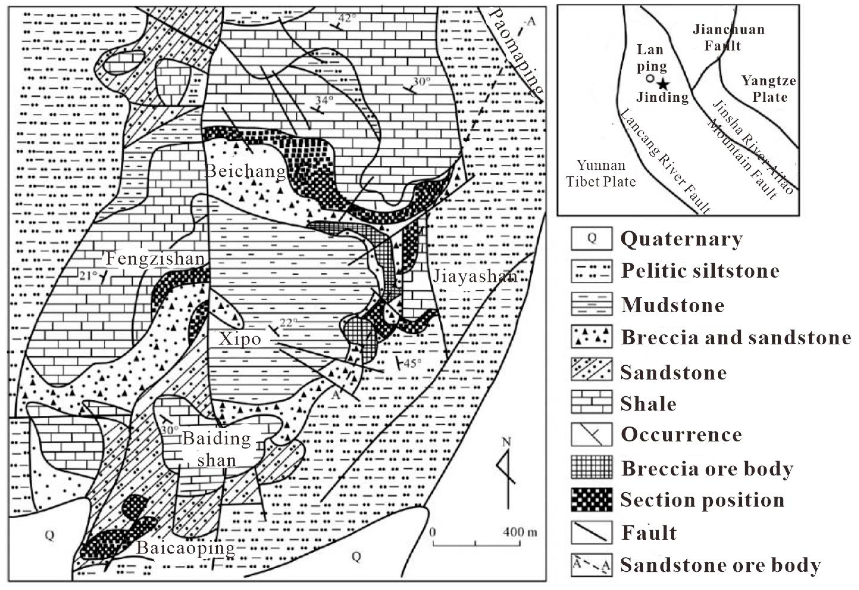
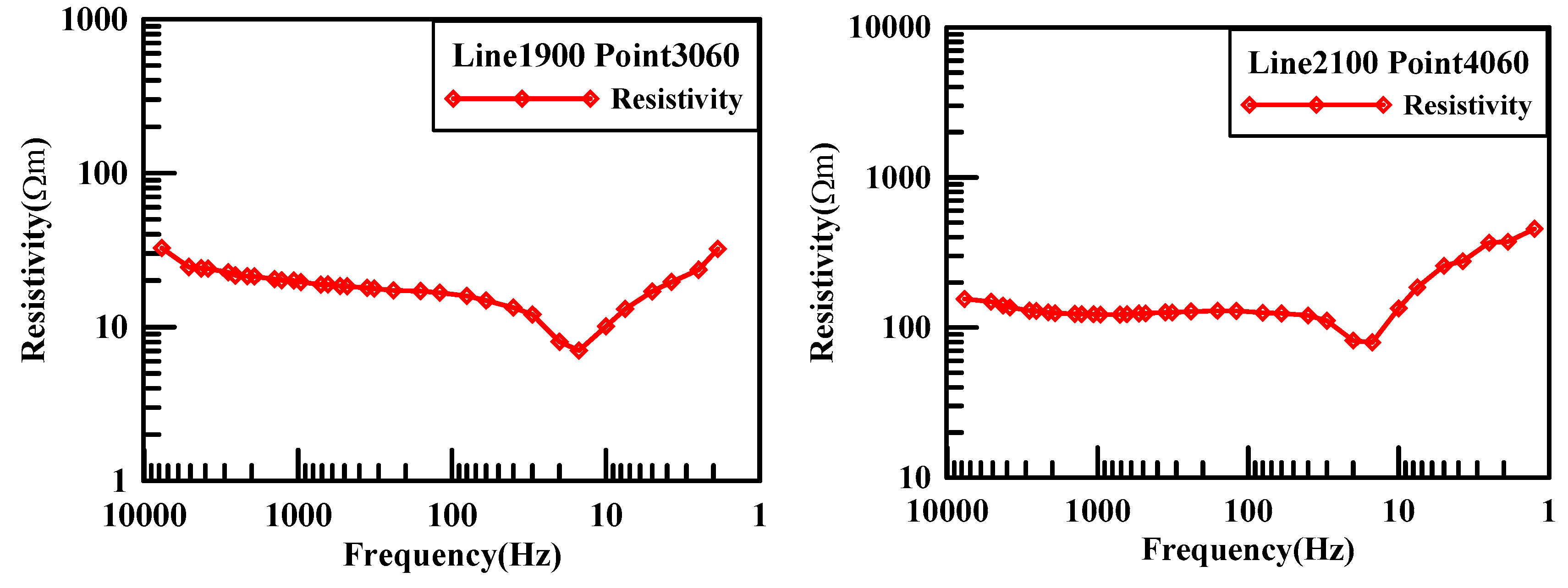
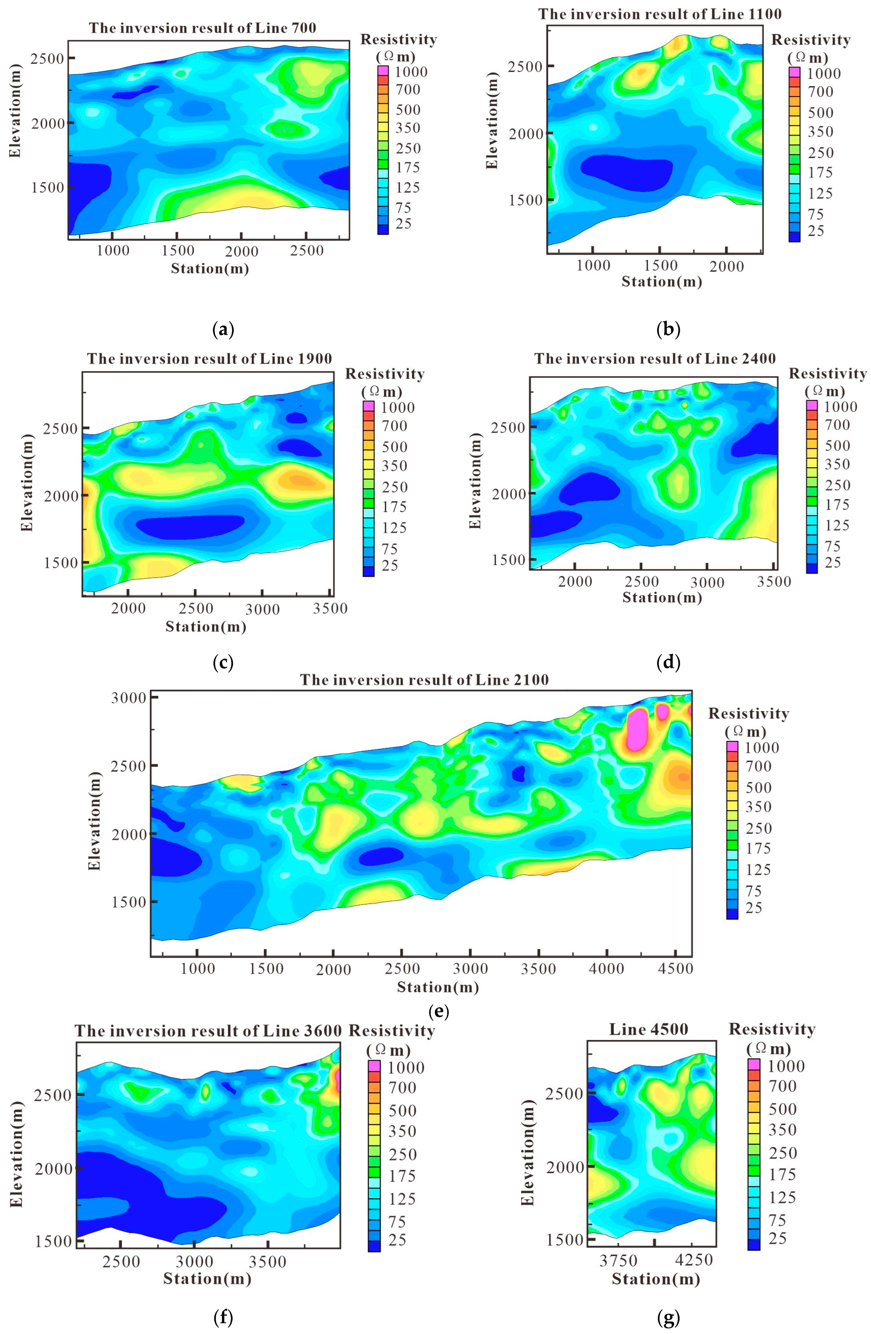
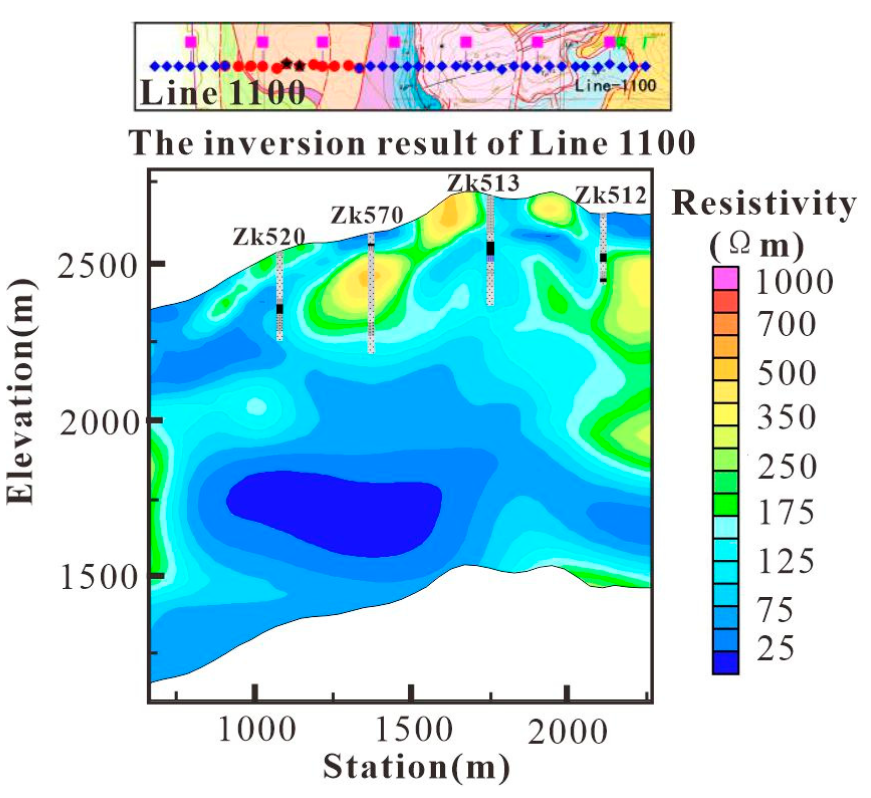
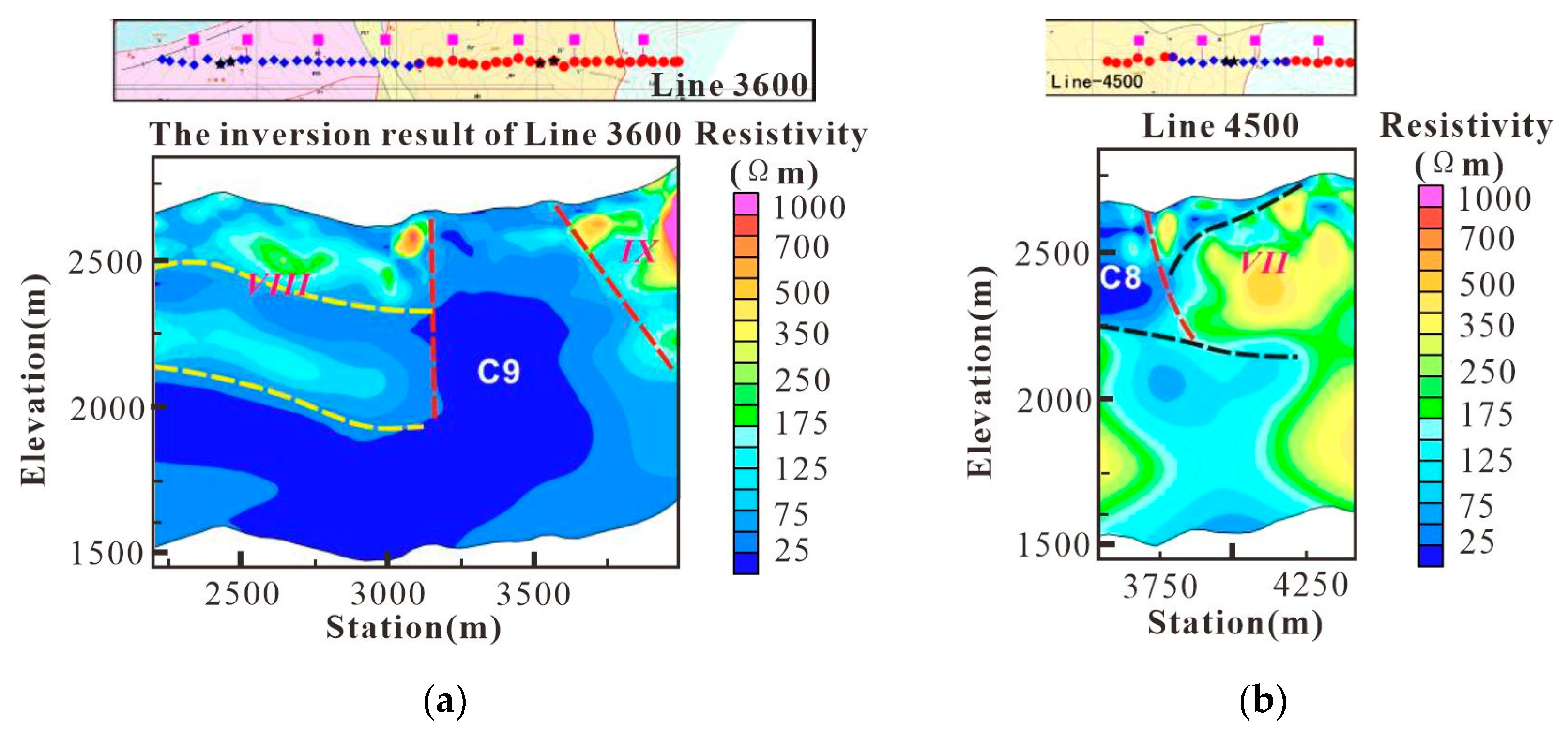
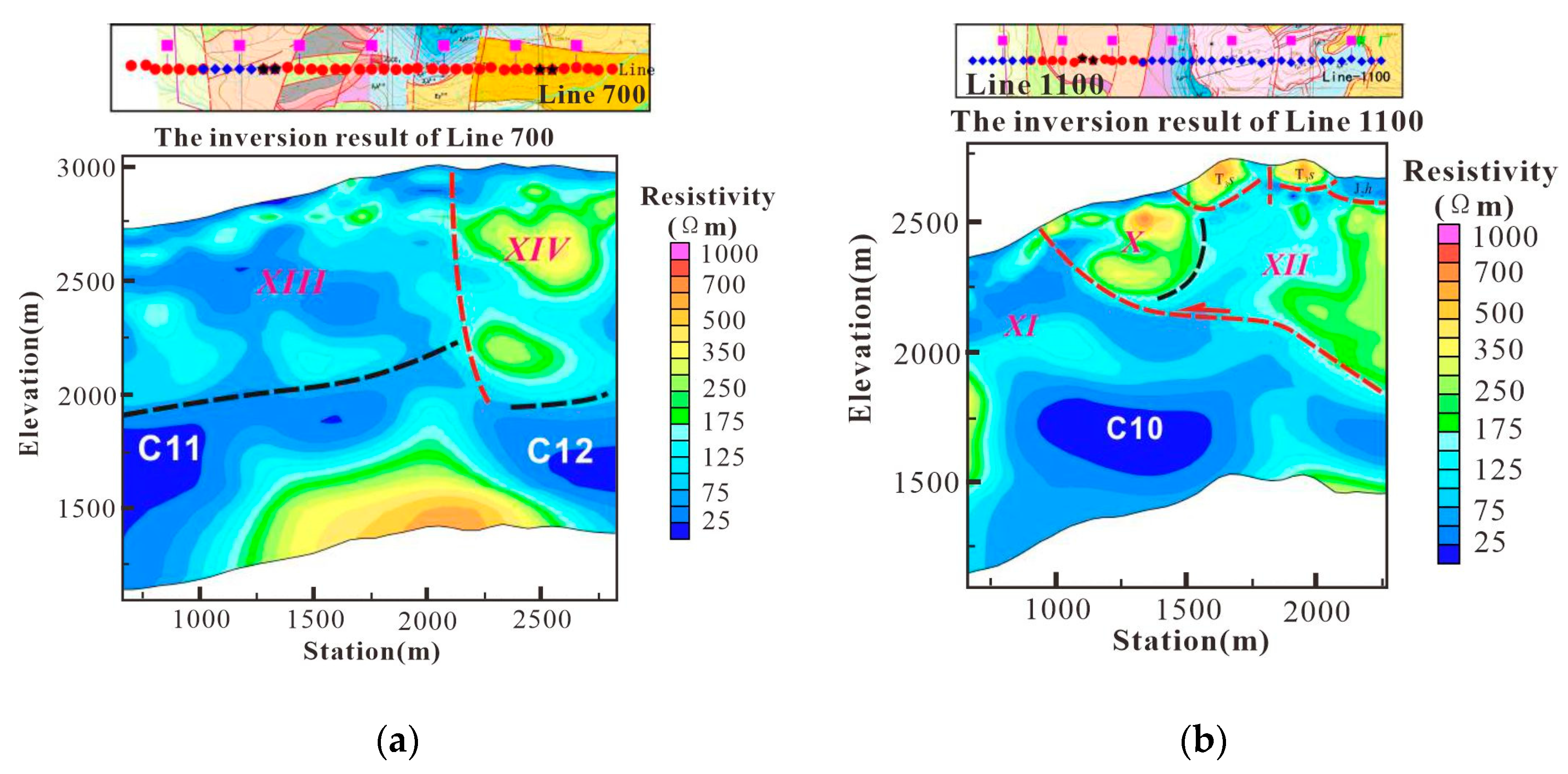
2.1. Geological Overview of the Deposit
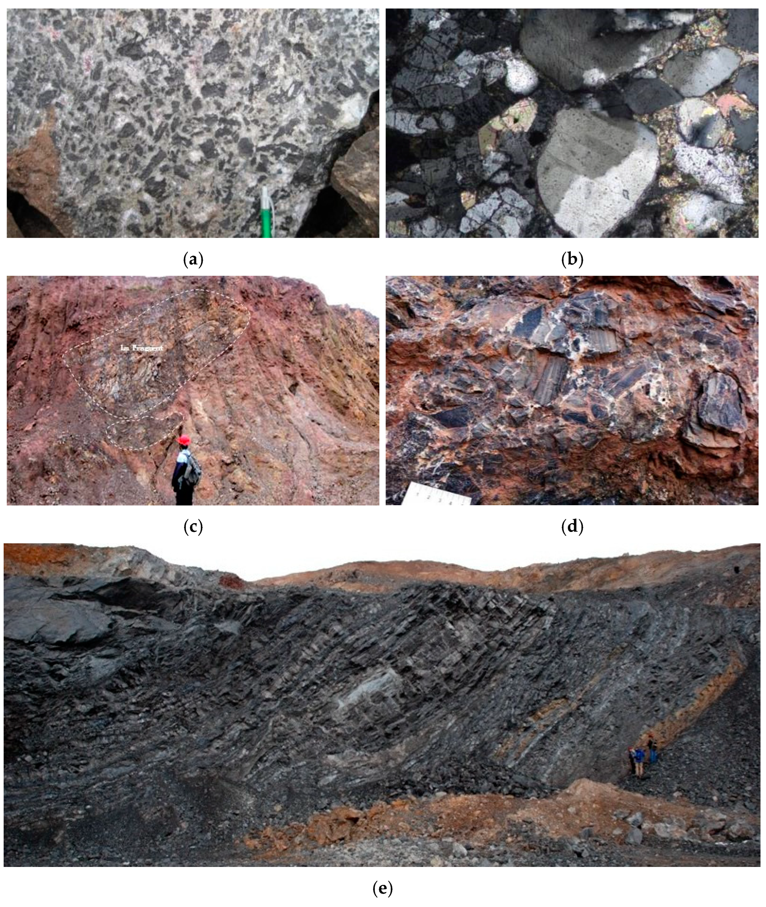
The Jinding Lead-Zinc Deposit is prominently situated within the densely compressed middle segment of the Sanjiang Fold System, positioned precisely at the northern terminus of the Lanping-Simao Meso-Cenozoic depression. It is strategically positioned between the north-south oriented faults tightly hemmed in by the Mishahe Fault Zone and the Lancang River Fault Zone, and is found to the western flank of the Bihe River Fault Zone, within the ancient Lanping-Yunlong Paleocene graben basin.The deposit is meticulously divided into seven distinct mining sections, including Beichang, Jiayashan, Fengzishan, Paomaping, Xipo, Nanchang, and Baicaoping. The mining area exposes a succession of strata ranging from the older to the younger, comprising the Upper Triassic Sanhedong Formation (T3s) of marine limestones (including brecciated limestones, dolomitic limestones, argillaceous limestones, and limestone mudstones), the Maichuqing Formation (T3m, the core strata of the syncline, with alternating layers of quartz sandstones and carbonaceous mudstones), the Middle Jurassic Huakaizuo Formation (J2h, interbedded layers of argillaceous siltstones, siltstones, and mudstones), the Upper Jurassic Bazhulu Formation (J2b, consisting of mudstones, argillaceous siltstones, and calcareous conglomerates), the Lower Cretaceous Jingxin Formation (K1j, with alternating layers of quartz sandstones, silty mudstones, and intercalated limestone conglomerates), the Upper Cretaceous Nanxin Formation (K2n, composed of argillaceous conglomerates, fine sandstones, siltstones, and mudstones), the Upper Cretaceous Hutousi Formation (K2h, characterized by long quartz sandstones), the Lower Tertiary Paleocene Yunlong Formation (E1y, interbedded layers of muddy gravelly rocks and argillaceous siltstones), the Guolang Formation (E2g, with alternating layers of argillaceous siltstones, silty mudstones, and intercalated fine sandstones), the Eocene Baoxiangsi Formation (Eb, featuring long quartz sandstones, conglomerates, sandstones, mudstones, and quartzites), the Upper Tertiary Pliocene Sanying Formation (N2s, with interbedded layers of conglomerates, sandy conglomerates, sandstones, and mudstones), and the Quaternary Pleistocene (Qp, sand and gravel layers) and Holocene (Qh, comprising gravels, sand grains, and sandy clays).
Figure 1.
Simplified Geological Map of the Jinding Mining Area, Yunnan Province.
Figure 1.
Simplified Geological Map of the Jinding Mining Area, Yunnan Province.
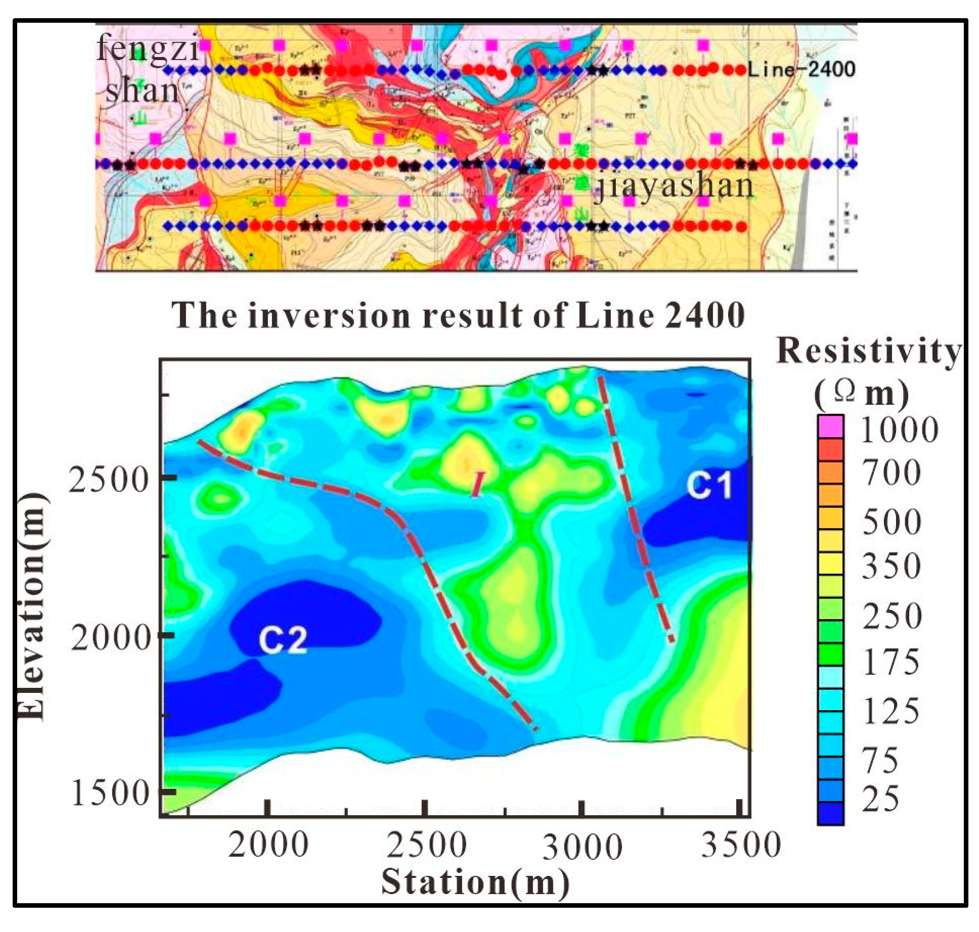
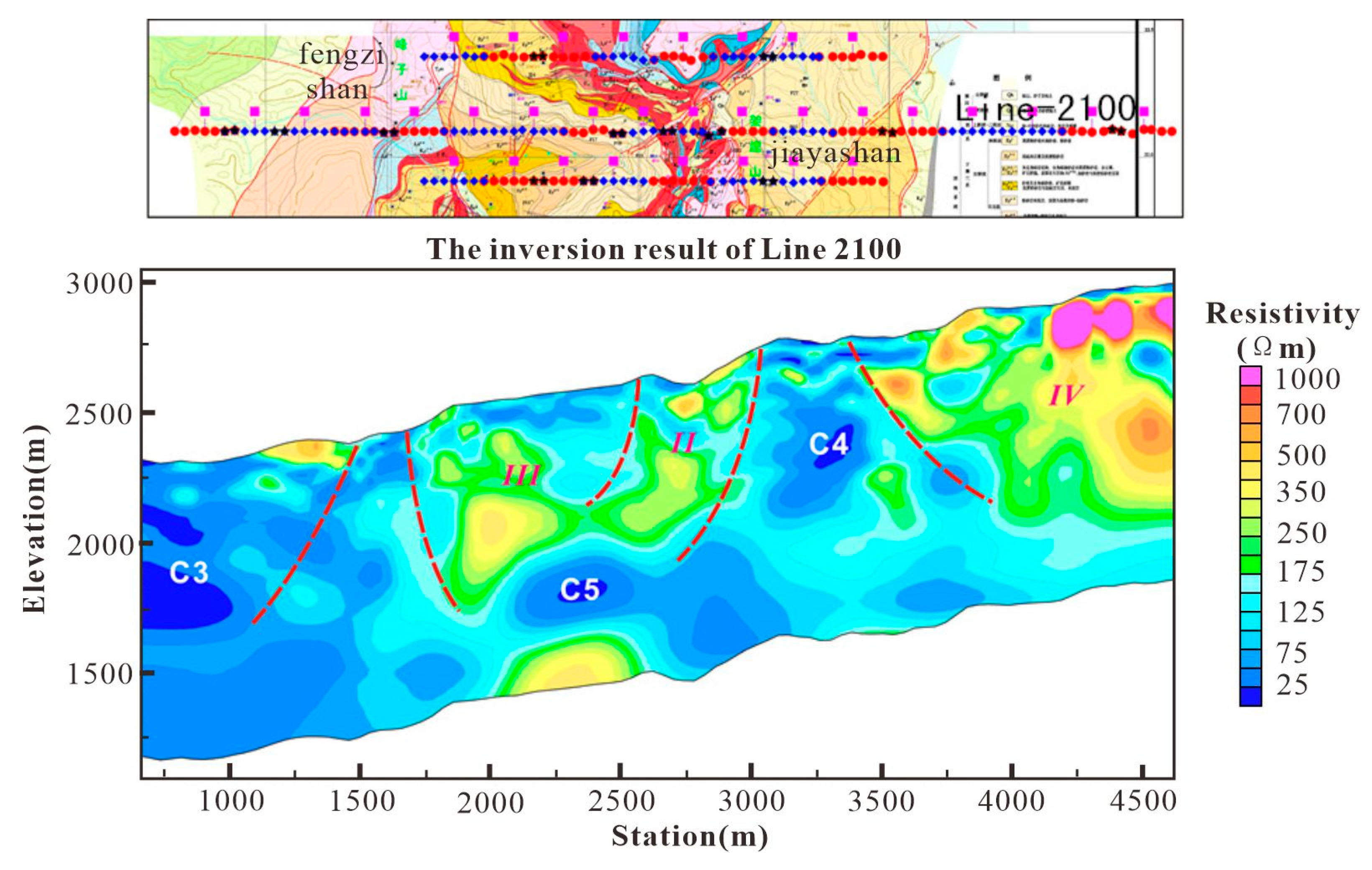
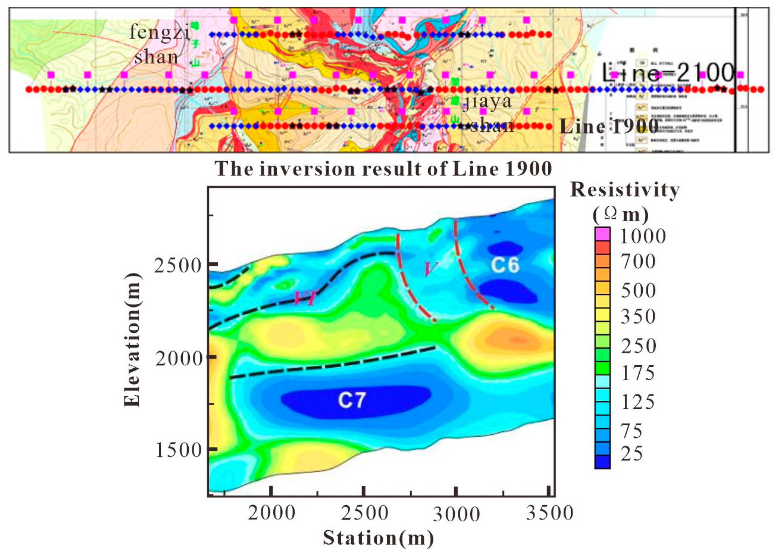
The primary geological structure of the mining area is a thrust nappe tectonic assemblage, which constitutes a significant component of the large-scale thrust nappe structure that formed during the Paleocene Yunlong period in the Lanping Basin. Klippe structures, or flysch formations, exist in numerous segments throughout the mining area. Furthermore, the thrust-sliding planes have also been incorporated into the tectonic domes, resulting in the formation of dome structures that are characterized by the co-deformation of both thrust tectonics and in-situ systems. In accordance with the preceding findings, it can indeed be concluded that the thrust tectonics predate the formation of the dome structures, with their inception likely commencing as early as the late Yunlong period. In summary, the geological structures of the Jinding mining area are complex, characterized by well-developed folds and faults that exhibit multiple stages of activity. This underscores the dynamic and protracted geological history of the region. The geological structures of the mining area are primarily characterized by the Gaoping-Laomujing syncline, the Bihe River Fault, horizontal thrust faults, transverse faults, oblique faults, and secondary fault structures.
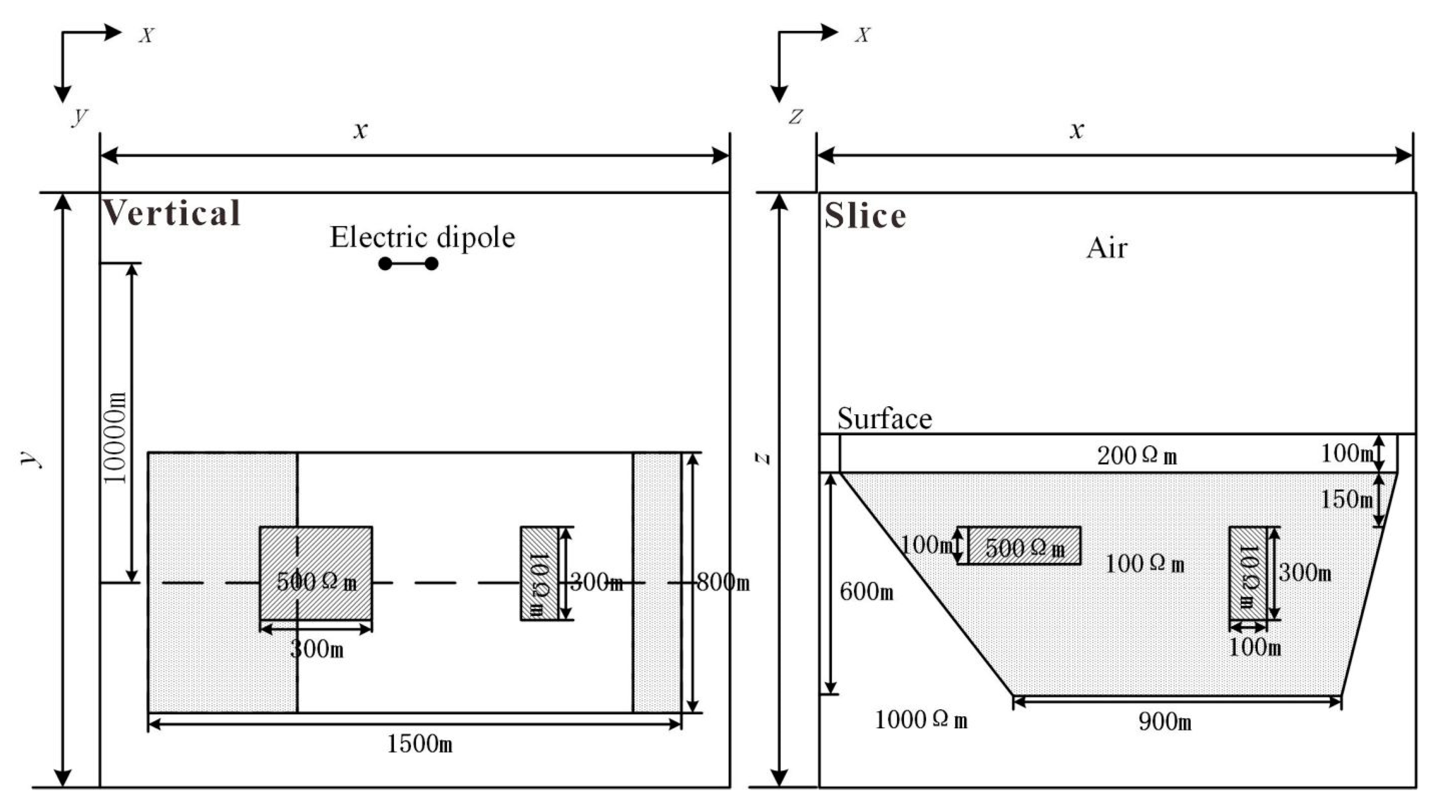
2.2. Geological and Geophysical Model of the Ore Deposit
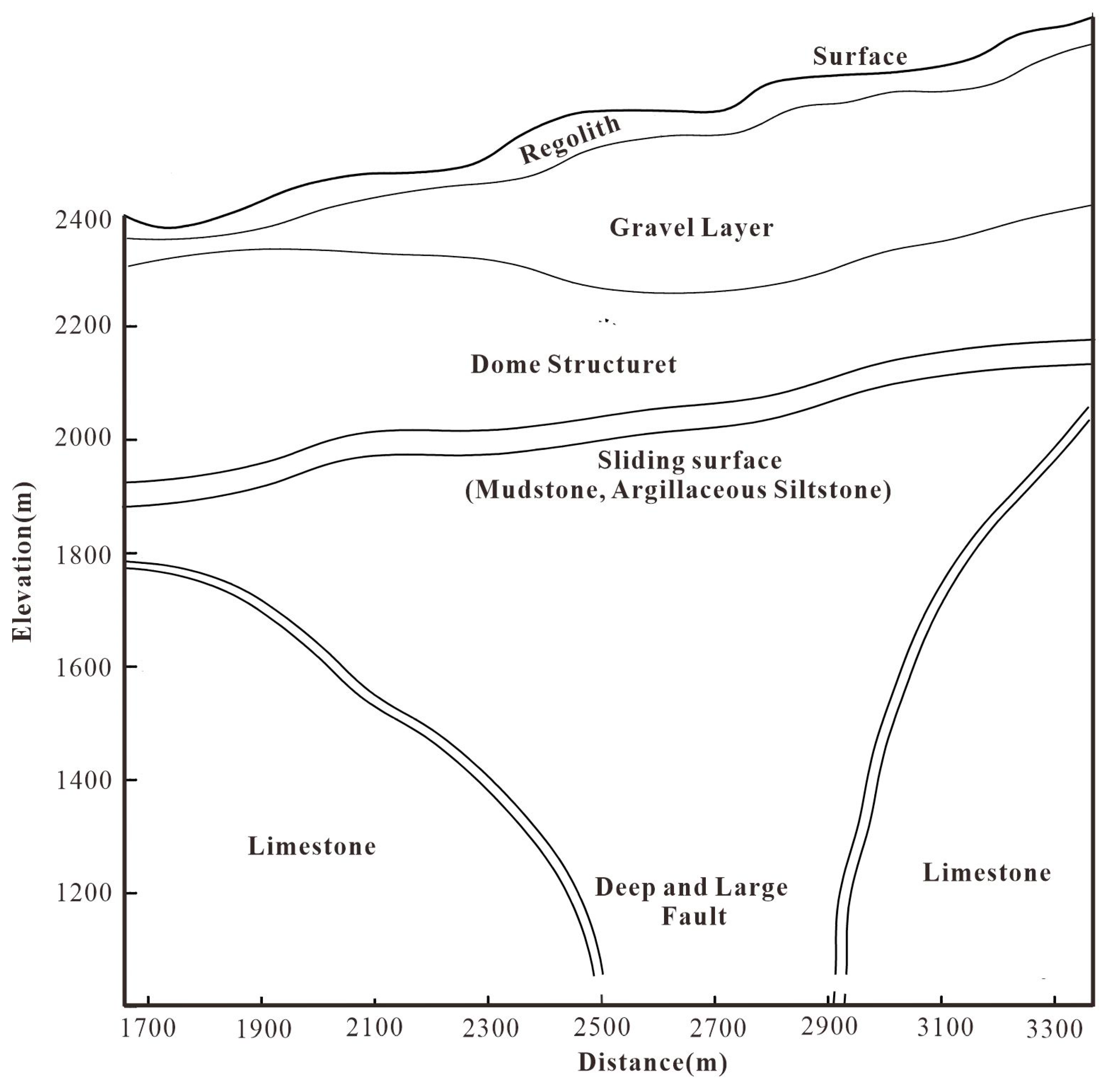
Based on the existing geological data, physical property measurement and 2D geological model[
15] (
Figure 2), we have constructed a 3D geophysical model of Jinding lead-zinc deposit, as shown in the
Figure 3.
In the
Figure 3, the first layer represents the surface covering layer with a thickness of 100m. Its main component is sand and gravel strata, and it has an average resistivity of 200
. Beneath the covering layer lie domes and concealed deep fault structures with a resistivity of 100
. On both sides of the fault are high-resistance surrounding rocks with a resistivity of 1000
. The ore bodies are hosted within the dome structure, primarily consisting of sandstone-type and limestone breccia ore bodies. The sandstone ore body resembles a platy form, with a resistivity of 500
. Its dimensions are 300m in length, 100m in width, and 300m in height. The limestone breccia ore bodies often appear as inclined or vertical thin layers, also with a resistivity of 500
, and their dimensions are 100m in length, 300m in width, and 300m in height. The limestone breccia ore bodies often occur as inclined or vertical thin layers with a resistivity of 500
. Their dimensions are typically 100m in length, 300m in width, and 300m in height.
2.3. The Coupled Finite-infinite Element Method of CSAMT
Numerical simulation research not only enhances people's understanding and knowledge about the exploration methods, but also assists in selecting the correct exploration approach and setting appropriate field acquisition parameters. Therefore, we employed a three-dimensional CSAMT forward modeling program, based on the coupled finite-infinite element method to conduct a numerical simulation on the geophysical model of Jinding lead-zinc mine. The 3D CSAMT forward modeling using the finite-element and infinite-element coupling method is an efficient numerical simulation technique for electromagnetic fields, which combines the advantages of the finite element method in handling complex geological structures and boundary conditions with the characteristics of the infinite element method in simulating infinite far-field attenuation. This method achieves rapid and high-precision forward modeling, reduces the computation domain and the number of nodes, accelerates the computation, and is of great significance to the development of exploration geophysics[
20,
21].
2.3.1. Fundamental Equation
The electric field generated by a horizontal electric dipole ( time factor
, angular frequency
) in an isotropic conductive medium satisfies the double curl equation [
22]:
where
is the resistivity,
is the current density vector of the electric dipole, and the magnetic permeability
of both the air and the subsurface medium is taken as the vacuum magnetic permeability, while the dielectric constant
is the vacuum dielectric constant.
The electric dipole source exhibits singularity. The total electric field is decomposed into the sum of the background field
(primary field ) and the induced field
(secondary field ). The background field
is directly solved using a one-dimensional geoelectric model[
23], while the induced field
is solved using the finite element method to avoid the calculation of source singularity.
The background field
also satisfies the double curl equation of the electric field. Equations (1) and (2) can be used to derive the double curl equation based on the secondary field
:
where
. We know that on an electrical interface, the normal component of the electric field is discontinuous, while nodal finite elements require the electromagnetic field to be continuous in the normal direction. Therefore, the obtained finite element solution is often inaccurate and needs to be corrected. In the source region, the electric field solution of nodal finite elements does not satisfy condition
; in the source-free region, it does not satisfy condition
. A divergence correction condition needs to be added to Equation (3) [
24].
2.3.2. Weak Solution Integral Form
Based on the weighted residual finite element method (Jin 2014), establish the residual formula for Equation (4):
Take any test function
, on the region
:
Let S be the outer boundary surface of the region
. Instead of using traditional truncated boundary conditions, infinite elements are employed. Within the infinite elements, the electromagnetic field decays to zero, so we have:
By applying the first vector Green's theorem, Equation (6) can be simplified to:
Use finite element method to discretize the internal computation domain. Assuming there are n nodes in the internal computation domain, the j-th test function can be taken as:
2.3.3. The Coupled Finite-Infinite Element Method
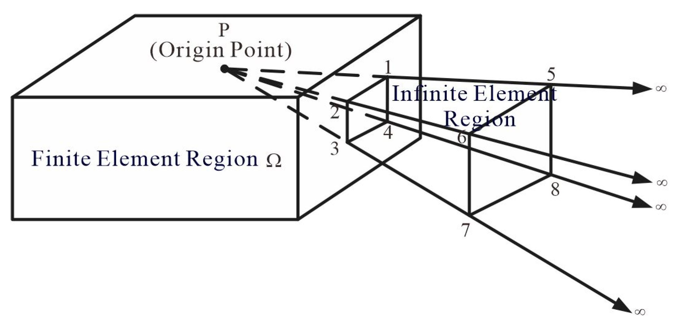
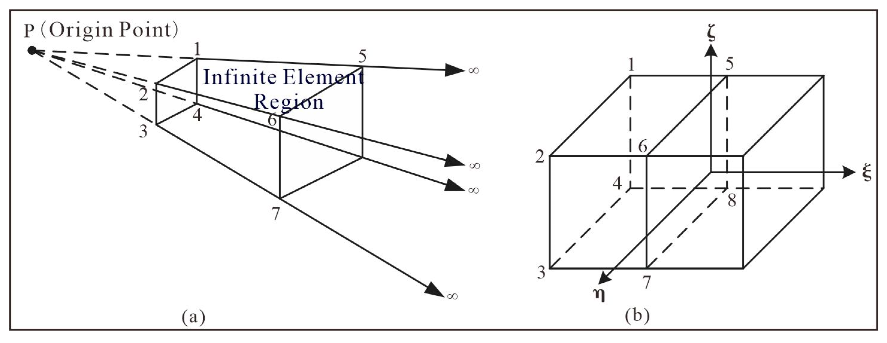
The coupled finite-infinite element method divides the entire solution domain into a finite element region and an infinite element region, replacing the traditional outer boundary with the infinite element region. Finite element analysis and infinite element analysis are performed in the two regions respectively, and they are combined through the assembly of the overall stiffness matrix for numerical solution.
Figure 4 is a schematic diagram of the division of finite element and infinite element calculation regions. In the figure, the finite element region is the target region, which includes the field source, target body, measurement points, etc.; the infinite element region extends from the boundary of the finite element region to infinity, serving as the boundary calculation region. Infinite element analysis involves using infinite element mapping and shape functions in a certain direction within this region to map the global coordinates to local coordinates. Its principle is the same as that of finite element analysis.
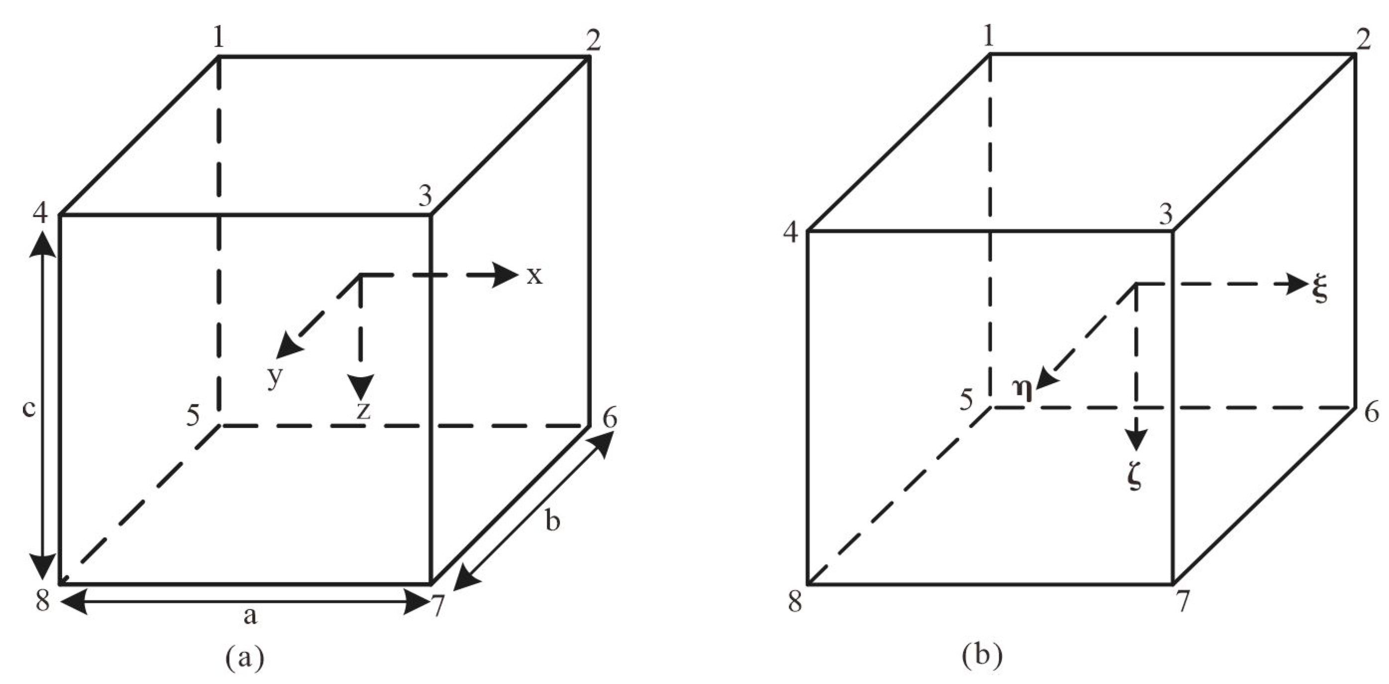
When performing finite element analysis, the rectangular hexahedron is used for regional discretization, and the element node numbering and coordinates are shown in
Figure 2.
In
Figure 5, the corresponding relationship between the coordinates of the parent and child elements is as follows:
Where
,
,
represent the midpoint of the child element, and a, b, c represent the three side lengths of the child element. The expression for the shape function of the rectangular hexahedron is as follows:
In the equation, , , represent the coordinates of node i in the child element within the parent element.
- 2.
The Infinite Element Analysis
When performing infinite element analysis, a three-dimensional eight-node Astley-type infinite element is used[
25].
Figure 3 is a schematic diagram of three-dimensional infinite element mapping, where nodes 1, 2, 3, 4, 5, 6, 7, and 8 are the basic elements of the infinite element. P is the coordinate origin, and nodes 1, 2, 3, and 4 are the four nodes of a finite element on the boundary. The distances from point P to nodes 5, 6, 7, and 8 are twice the distances from point P to nodes 1, 2, 3, and 4, respectively. Infinite element analysis involves mapping infinite coordinates to local coordinates in
Figure 3(b) through infinite element mapping. In
Figure 3(b), the four outermost nodes of the infinite element represent infinity, and their field values are zero.
In
Figure 3(b),
represents the mapping direction of the infinite element. Within plane
, the infinite element and the finite element adopt the same mapping form and shape function. The coordinate mapping for the infinite element is as follows:
Li represents the area of the quadrilateral,
Combining the coordinate mapping relationship in direction
, the coordinate mapping function for the 8-node infinite element can be obtained:
Where:
quadrilateral surface element mapping and linear interpolation of area coordinates
For the shape function of the infinite element, its specific expression is as follows:
This shape function is the product of the coefficient A used in the shape function adopted in the Astley Mapped Infinite Element Theory (Astley, 1994) and a second-order Lagrange interpolation polynomial.
The finite element and infinite element analysis are basically consistent, both being eight-node elements. Therefore, in numerical simulations, the infinite elements and finite elements can be perfectly combined to ensure the symmetry of the stiffness matrix, making the solution simple and convenient.
2.3.4. Solving the Equation System
In the three-dimensional numerical simulation of CSAMT, each node has three degrees of freedom in the x, y, and z directions. Therefore, we take:
Where, is the shape function of the j-th measurement point, and its specific form is detailed in equations (11) and (14).
Equation (9) can be written as:
Using the vector curl formula and the divergence formula, Equation (16) above can be simplified and written in matrix form as follows:
where:
Equation (17) is a large, sparse, symmetric complex coefficient linear equation system. In this system, matrix A represents the overall stiffness matrix of the coupled finite element-infinite element method, which is an order square matrix. Here, , , enote the total number of nodes in the x, y, and z directions, respectively. Each row in matrix A has a maximum of 81 non-zero elements. x represents the electric field values at each node that need to be solved; b is the right-hand side term, which includes the anomalous body and the primary field. For solving large-scale sparse linear equation systems, this paper adopts Pardiso, an open-source solver with excellent performance and high parallelization. Pardiso uses LU decomposition for direct solving, making it particularly suitable for handling multi-source CSAMT problems.
2.4. The Forward Modeling of the Jinding Lead-Zinc Geophysical Model
We use the coupled finiment-infiniment element method, the forward modeling calculation parameters are as follows:
In the x direction, the subdivision area ranges from -3000 to 15000. Within the survey line area, the grid size is set to 50 meters, resulting in a total of 121 nodes.
In the y direction, the subdivision area ranges from -3000 to 3000. Within the survey line area, the grid size is set to 50 meters, resulting in a total of 63 nodes. Near the field source and the target body, the grid subdivision is relatively dense.
In the z direction, the subdivision area ranges from -3200 to 3000, with a total of 36 nodes. The air region spans from -3200 to 0, and is subdivided into 6 layers. Due to the rapid attenuation of the field in underground media, the grid subdivision size is smaller, the grid size is set to 25 meters.
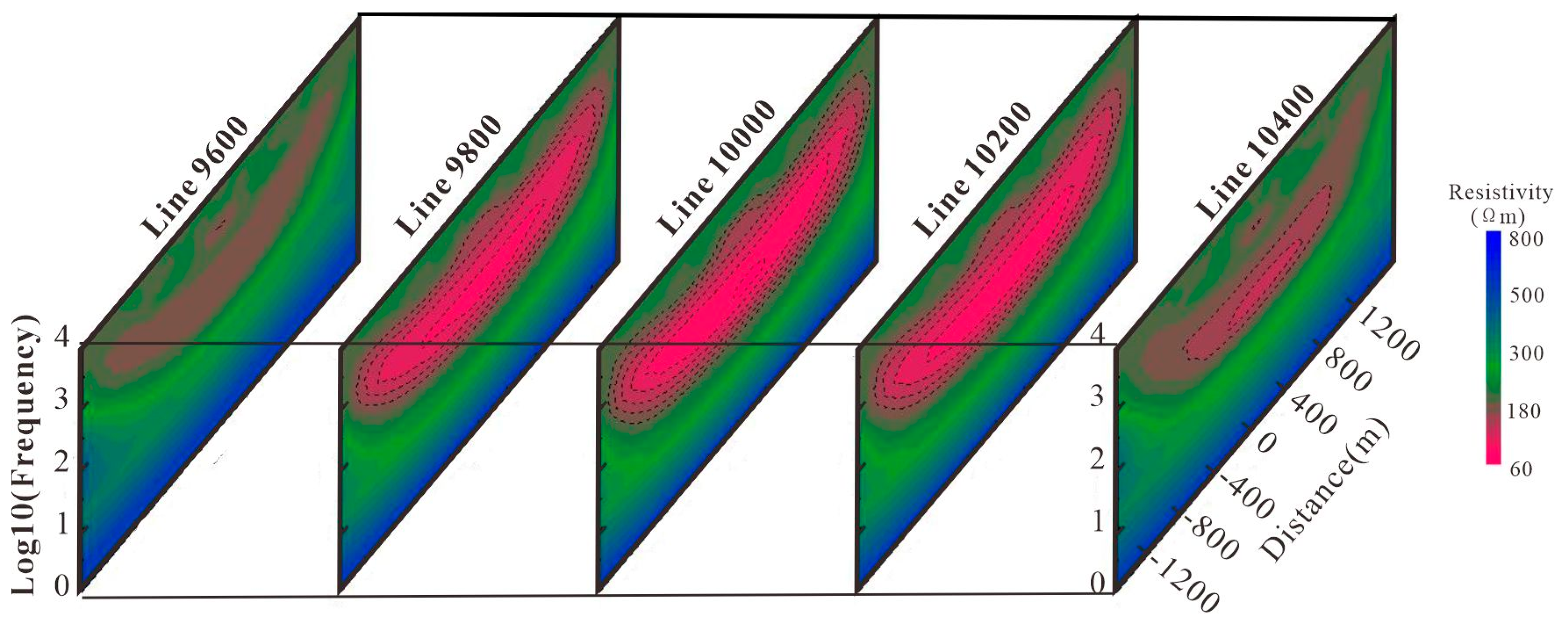
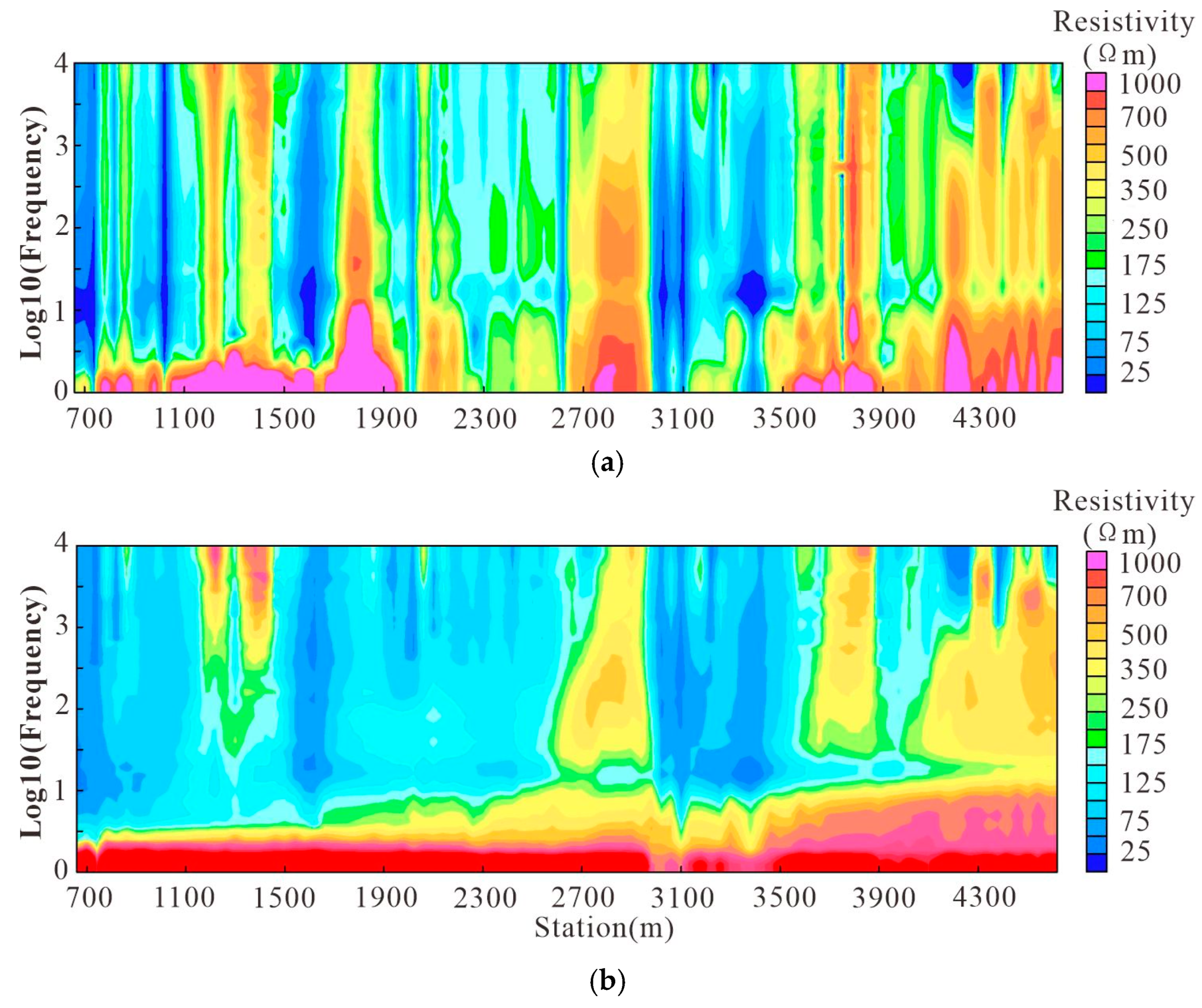
Frequencies: 8192, 4096, 2048, 1024, 512, 256, 128, 64, 32, 16, 8, 4, 2, 1 Hz, totaling 14 frequencies. The average calculation time for each frequency point is approximately 240 seconds. The numerical simulation results are presented in
Figure 4.
In
Figure 7, from left to right, the vertical source-receiver distances of the five survey lines are 9600m, 9800m, 10000m, 10200m, and 10400m, respectively. From the apparent resistivity pseudo-section map , it can be observed that the CSAMT 3D forward modeling results exhibit a significant response to the low-resistivity dome structure of the Jinding lead-zinc deposit, and provides a clear reflection to the structure's morphology. However, due to the boundary effects, the boundary between the dome structure and the high-resistivity limestone is relatively blurred. In addition, due to the low-resistivity shielding effect of electromagnetic methods, the relatively high-resistivity lead-zinc ore bodies show little response in the simulation. Based on the numerical simulation results, it can be seen that when exploring for high-resistivity target bodies in low-resistivity surrounding rocks, the CSAMT electromagnetic response is weak, and the numerical effect is not significant. However, when exploring for low-resistivity structures such as faults and fracture zones in high-resistivity surrounding rocks, the effect is very pronounced. Therefore, it is feasible to conduct CSAMT exploration research in the Jinding lead-zinc mining area to identify low-resistivity faults, dome structures, and other features within the ore deposit.
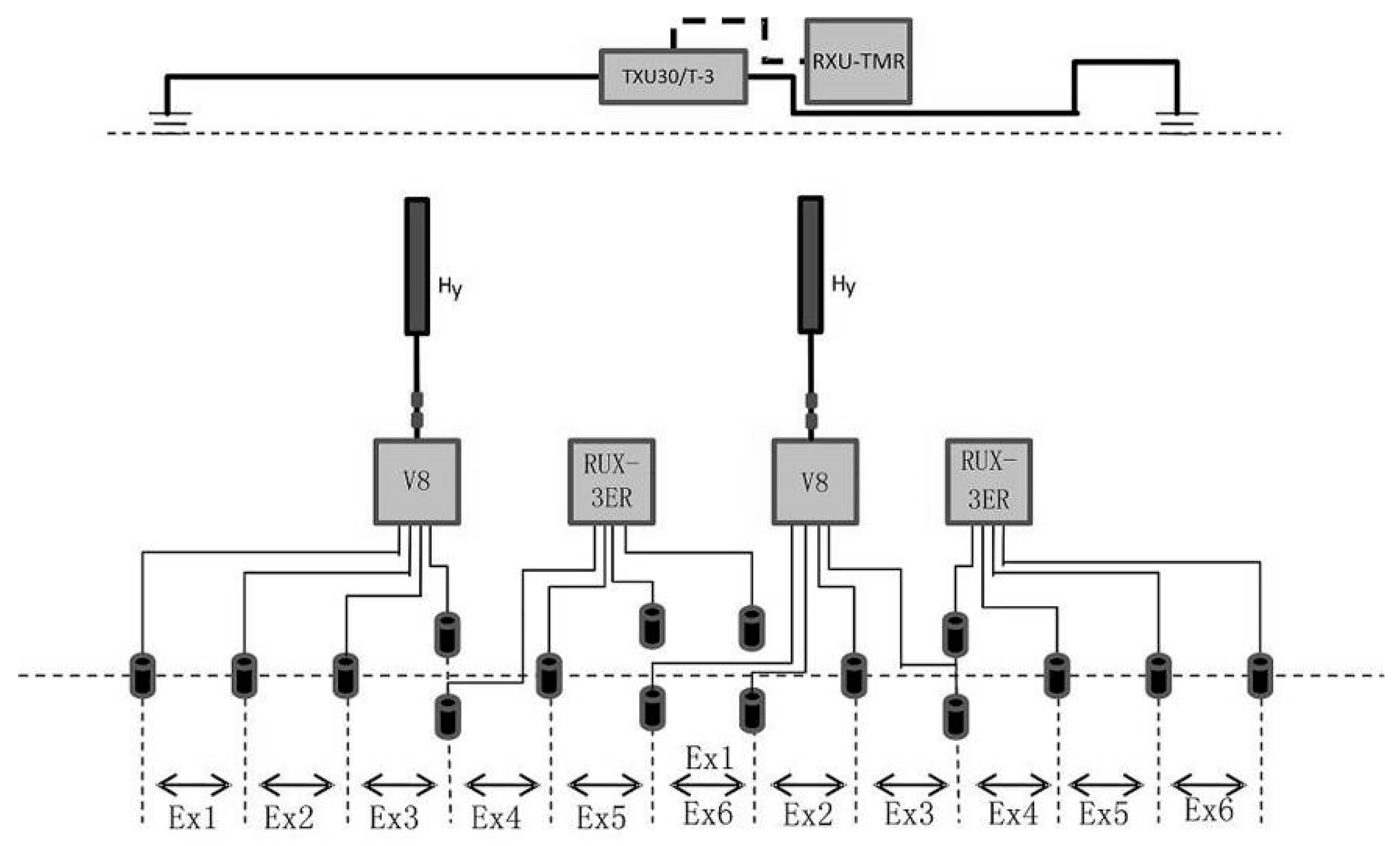
Additionally, the forward modeling parameters used in the 3D CSAMT numerical simulation, such as grid size, vertical source-receiver distance, frequency band range, survey line length, as well as the three-dimensional size and location of the target body, can assist us in designing the field CSAMT acquisition parameters to achieve good exploration results.