Submitted:
28 February 2025
Posted:
06 March 2025
You are already at the latest version
Abstract
Software defect prediction aims to identify defect-prone modules before testing, reducing costs and duration. Machine learning (ML) techniques are widely used to develop predictive models for classifying defective software components. However, high-dimensional training datasets often degrade classification accuracy and precision due to irrelevant or redundant features. To address this, effective feature selection is crucial, but it poses an NP-hard challenge that can be efficiently tackled using heuristic algorithms. This study introduces a Binary Multi-Objective Starfish Optimizer (BMOSFO) for optimal feature selection, enhancing classification accuracy and precision. The proposed BMOSFO balances two conflicting objectives: minimizing the number of selected features and maximizing classification performance. A Choquet Fuzzy Integral-based Ensemble Classifier is then employed to further enhance prediction reliability by aggregating multiple classifiers. The effectiveness of the proposed approach is validated using five real-world NASA benchmark datasets, demonstrating superior performance compared to traditional classifiers. Experimental results reveal that key software metrics—such as design complexity, operators and operands count, lines of code, and number of branches—significantly influence defect prediction. The findings confirm that BMOSFO not only reduces feature dimensionality but also enhances classification performance, providing a robust and interpretable solution for software defect prediction. This approach shows strong potential for generalization to other high-dimensional classification tasks.
Keywords:
Software Defect Prediction
; Feature Selection
; Binary Multi-Objective Optimization
; Starfish Optimization Algorithm
; Fuzzy Ensemble Learning
; Choquet Integral
; Machine Learning
; Artificial Neural Networks
; Heuristic Algorithms
; Software Metrics
1. Introduction
The presence of defects in software systems poses a significant challenge in modern software engineering, affecting software reliability, maintainability, and security. Software defects can lead to system failures, performance degradation, and increased operational costs, making their early detection a critical aspect of software quality assurance. As software complexity increases, the need for effective Software Defect Prediction (SDP) becomes more pressing. SDP aims to identify defect-prone software modules before testing and deployment, allowing developers to focus their efforts on these areas, thereby optimizing resource allocation and improving software quality [1,2].
Traditional defect detection methods, such as manual code reviews and testing, are often time-consuming, expensive, and prone to human error, especially in large-scale software projects [3]. Consequently, automated defect prediction techniques have gained significant attention, particularly those leveraging Machine Learning (ML) models. However, despite the promising results achieved by ML-based approaches, several challenges remain unresolved.
A critical issue is the high dimensionality of defect datasets, where numerous software metrics—such as complexity measures, lines of code, and structural properties—introduce redundancy and noise, leading to reduced classification performance [4,5]. Feature selection plays a key role in mitigating this problem by eliminating irrelevant and redundant features, thereby improving classification accuracy and generalizability. However, feature selection is an NP-hard problem, making exhaustive search methods impractical for large-scale datasets. To address this, evolutionary optimization algorithms have emerged as a promising solution, effectively identifying the most informative features for software defect prediction while reducing computational overhead.
Additionally, existing SDP approaches are often limited by their reliance on individual classifiers, which may suffer from overfitting and instability when trained on imbalanced defect datasets. Ensemble learning addresses this limitation by combining multiple classifiers to improve predictive performance. However, traditional ensemble techniques typically assume classifier independence and rely on simple aggregation methods, such as majority voting or averaging, which fail to account for interactions among classifiers. This can lead to suboptimal prediction accuracy, especially when classifiers exhibit correlated errors. Consequently, there is a need for advanced aggregation methods that can optimally fuse the outputs of multiple classifiers while considering their interdependencies.
To address these challenges, this study proposes a novel hybrid evolutionary fuzzy ensemble approach for software defect prediction. The proposed framework integrates two key components:
- Binary Multi-Objective Starfish Optimizer (BMOSFO) for Feature Selection: A binary multi-objective version of the Starfish Optimizer (BMOSFO) is introduced for feature selection, ensuring that only the most relevant software metrics are considered, improving classification performance. BMOSFO leverages the unique behaviors of starfish, such as regeneration and multidimensional movement, to balance exploration and exploitation in high-dimensional feature spaces. This enables effective navigation of complex feature subsets, achieving superior convergence speed and computational efficiency compared to conventional evolutionary algorithms.
- Choquet Fuzzy Integral-based Ensemble Classification: To enhance classification accuracy, a Choquet Fuzzy Integral-based Ensemble Classifier is developed. Unlike traditional ensemble methods that assume classifier independence, the Choquet Integral considers interactions among classifiers, enabling more informed decision fusion. By optimally aggregating multiple machine learning models, including K-Nearest Neighbors (KNN) [6], Support Vector Machines (SVM) [7,8], Decision Trees (DT) [9], Logistic Regression (LR) [10], Random Forest (RF) [11,12], Gaussian Naive Bayes (GNB) [13,14], and Artificial Neural Networks (ANN) [15,16,17], the Choquet Integral enhances defect prediction reliability by accounting for the interdependencies among classifiers.
The key contributions of this study are:
- Introduction of BMOSFO for Feature Selection: BMOSFO is designed to efficiently reduce feature dimensionality while maintaining high classification accuracy. It achieves this by balancing exploration and exploitation through unidimensional and five-dimensional search mechanisms, inspired by starfish regeneration and movement behaviors.
- Advanced Ensemble Classification: A Choquet Fuzzy Integral-based Ensemble Classifier is developed to optimally aggregate multiple ML models. By leveraging the Choquet Integral’s ability to account for interactions among classifiers, the ensemble method enhances prediction accuracy and robustness [18].
- Comprehensive Evaluation on Real-World Datasets: The proposed approach is rigorously evaluated on five real-world benchmark datasets, demonstrating superior performance compared to traditional feature selection and classification methods.
- Insightful Feature Impact Analysis: An in-depth analysis of the most impactful software metrics, including design complexity, number of operators and operands, development time, lines of code, commented lines, number of branches, and operand sum, is conducted to highlight their significance in defect prediction.
The proposed framework addresses the limitations of conventional defect prediction models by integrating evolutionary optimization and fuzzy ensemble learning, contributing to improved accuracy and interpretability in software defect classification. The approach not only enhances defect prediction performance but also provides actionable insights into the impact of key software metrics, facilitating more reliable software quality assurance practices.
The remainder of this paper is structured as follows. Section 2 presents a comprehensive review of related work on predictive modeling for software defect detection. Section 3 details the proposed methodology, including dataset descriptions, the Starfish Optimizer, the BMOSFO algorithm, and the functioning of the Choquet Fuzzy Integral-based ensemble classification. Section 4 describes the experimental setup, evaluation metrics, and benchmark techniques. Section 5 discusses the experimental findings, including an in-depth analysis of model performance and feature selection impact. Section 6 summarizes the study’s key findings, discusses limitations, and outlines potential future research directions in predictive modeling for software defect detection.
2. Related Work
This section provides an overview of related research in the area of software defect prediction, categorized into four primary approaches: (1) Machine Learning (ML)-based defect prediction, (2) Deep Learning (DL)-based approaches, (3) Evolutionary Algorithms, and (4) Ensemble Methods. Each category contributes to advancing defect prediction models by addressing challenges related to accuracy, feature selection, and model stability. This section critically analyzes key studies within these categories, highlighting their strengths, limitations, and the research gaps that motivate the proposed hybrid evolutionary fuzzy ensemble approach.
2.1. Machine Learning Approaches for Software Defect Prediction
Several studies have explored the use of machine learning models for software defect prediction. In [19], a tree-boosting algorithm (XGBoost) was employed to predict software defects using module features that are easily computable. A model sampling strategy was proposed to enhance explainability while maintaining predictive performance. A cloud-based architecture was developed in [20] to facilitate real-time software defect detection, incorporating four backpropagation training algorithms along with a fuzzy layer to optimize training function selection. Experimental results demonstrated the effectiveness of Bayesian regularization and scaled conjugate gradient methods in improving prediction accuracy.
Efforts have also been made to improve classification performance using hybrid approaches. A technique combining K-means clustering, classification models, and particle swarm optimization (PSO) was introduced in [21], demonstrating that SVM and its enhanced variant achieved the highest accuracy. Similarly, a meta-heuristic feature selection model utilizing random forest (RF), SVM, and PSO was evaluated in [22], where it was shown that feature dimensionality could be reduced by 75.15% while maintaining high classification accuracy. The impact of kernel functions on SVM-based defect prediction was analyzed in [23], where results indicated that utilizing the top 40% of selected features led to significant improvements in classification efficacy.
Traditional ML models often suffer from high-dimensional input spaces that introduce noise and redundancy, affecting classifier performance. In [7], different feature selection methods, including filter-based, wrapper-based, and hybrid approaches, were analyzed to determine their impact on classifier accuracy. Results showed that hybrid methods combining filter and wrapper techniques yielded the most significant performance gains. Another work [8] explored multi-objective feature selection techniques, demonstrating that optimization-based feature selection could further improve classification robustness while reducing computation time.
Although ML models have shown promising results, their performance is often hindered by the high dimensionality and redundancy of software metrics. This highlights the need for effective feature selection techniques, motivating the development of advanced evolutionary algorithms, as explored in this study.
2.2. Deep Learning Approaches for Software Defect Prediction
Deep learning techniques have gained attention for their ability to extract complex feature representations from software repositories. A neural network-based framework was introduced in [24] to predict software defects, achieving an 8% increase in squared correlation coefficient and a 14% reduction in mean square error compared to previous methods. Challenges related to context complexity and data scarcity in DL-based defect prediction were discussed in [25], where self-supervised training and Transformer-based architectures were suggested to enhance code comprehension and reduce labeled data dependency.
To improve software defect detection, a gated hierarchical long short-term memory (GH-LSTM) network was proposed in [26], leveraging hierarchical LSTM networks for extracting semantic features from abstract syntax trees (ASTs). Similarly, a BERT-based semantic feature extraction method combined with bidirectional long short-term memory (BiLSTM) networks was explored in [27]. Data augmentation techniques were employed to enhance training, leading to superior performance across ten open-source projects. A meta-analysis of 102 peer-reviewed studies on deep learning-based defect prediction was conducted in [28], emphasizing the need for replication packages, diverse software artifacts, and data augmentation to improve generalizability.
Recent studies have further examined the applicability of pre-trained deep learning models for software defect detection. Transformer-based architectures, including BERT and CodeBERT, have been evaluated for their ability to extract meaningful representations of code artifacts. Another study [17] focused on the integration of graph neural networks (GNNs) with deep learning models, leveraging software dependency graphs to improve feature learning for defect prediction.
Despite their superior feature extraction capabilities, DL models are challenged by data scarcity and context complexity in defect prediction tasks. This study addresses these limitations by integrating DL with fuzzy ensemble methods to enhance generalization and robustness.
2.3. Evolutionary Algorithms for Software Defect Prediction
Evolutionary computation techniques have been widely applied to enhance software defect prediction. In [29], a hybrid method combining genetic algorithms (GA), SVM, and PSO was implemented across 24 datasets, including NASA MDP and Java open-source repositories. The results showed improved classification performance on both small and large datasets. A supervised differential evolution-based approach (DEJIT) was introduced in [30] for just-in-time software defect prediction (JIT-SDP), leading to substantial improvements in effort-aware prediction.
Further advancements have focused on optimizing evolutionary search strategies. In [31], a hybrid model combining the sparrow search algorithm (SSA) with PSO (SSA-PSO) was designed to accelerate convergence and improve classification accuracy. The Genetic Evolution (GeEv) framework was introduced in [32] to enhance feature selection diversity by evolving random offspring with higher survival potential. Similarly, a novel three-parent genetic evolution method (3PcGE) was proposed in [33], demonstrating superior classification performance compared to conventional wrapper and filter-based feature selection methods.
Recently, hybrid evolutionary approaches have been explored to optimize defect prediction models further. In [18], a parametric evolutionary technique was applied to dynamically adjust hyperparameters in defect prediction models. The study highlighted the advantages of adaptive evolutionary strategies over static parameter tuning, demonstrating improved model generalization and efficiency.
While existing evolutionary algorithms improve feature selection, they often suffer from slow convergence and premature stagnation. This motivates the introduction of BMOSFO, which leverages multidimensional search strategies inspired by starfish regeneration to enhance convergence speed and exploration capabilities.
2.4. Ensemble Approaches for Software Defect Prediction
Ensemble learning has been widely adopted in software defect prediction due to its ability to enhance classification accuracy by combining multiple models. Bagging, boosting, and stacking have been shown to mitigate overfitting while improving prediction robustness [34,35,36]. In [37], an ensemble multiple kernel correlation alignment (EMKCA) method was introduced for heterogeneous defect prediction. The approach applied kernel classifiers to transform the data distribution and address class imbalance, outperforming benchmark methods across 30 datasets.
A comparative evaluation of deep learning and machine learning models for defect classification was conducted in [38], where ensemble techniques, including bagging, boosting, and stacking, achieved superior predictive performance compared to standalone classifiers. In [39], a two-stage ensemble model was developed, integrating random forest (RF), support vector machines (SVM), Gaussian Naive Bayes (GNB), and artificial neural networks (ANN), with final predictions determined using a voting ensemble. Similarly, a hybrid SMOTE-Ensemble method was introduced in [40], employing bagging, RF, and AdaBoost to enhance classification performance in imbalanced datasets.
Additional advancements in ensemble learning include the use of principal component analysis (PCA) for feature selection, as demonstrated in [41]. A framework integrating PCA with ensemble classifiers showed that bagging achieved the highest classification accuracy of 91.49%, with feature reduction leading to an additional 0.6% increase in performance. An ensemble learning strategy combining KNN, RF, and ANN was proposed in [42], demonstrating superior performance over individual classifiers.
Although ensemble learning enhances classification accuracy, traditional methods assume classifier independence, leading to suboptimal aggregation when classifiers exhibit correlated errors. The Choquet Fuzzy Integral addresses this by modeling interdependencies, enabling more informed decision fusion, as explored in this study.
In summary, while significant progress has been made in ML, DL, evolutionary, and ensemble approaches for software defect prediction, challenges related to feature selection, classifier interdependencies, and generalization remain unresolved. This study addresses these gaps by introducing a hybrid evolutionary fuzzy ensemble approach, leveraging BMOSFO for multi-objective feature selection and the Choquet Fuzzy Integral for advanced ensemble classification.
3. Proposed Hybrid Model for Software Defect Prediction
This section presents the proposed software defect prediction model, which integrates machine learning classifiers with Binary Multi-Objective Starfish Optimization (BMOSFO) for feature selection. The BMOSFO algorithm is employed to identify the most relevant software defect features, improving classification accuracy and computational efficiency. The machine learning models used in this study include Artificial Neural Networks (ANN), Decision Trees (DT), Random Forest (RF), K-Nearest Neighbors (KNN), Naive Bayes (NB), Logistic Regression (LR), and Support Vector Machines (SVM). Furthermore, an ensemble classifier based on the Choquet Fuzzy Integral is applied to aggregate predictions and enhance defect classification performance.
The integration of BMOSFO for feature selection with the Choquet Fuzzy Integral-based ensemble classification presents a novel approach in software defect prediction. This combination leverages the exploration-exploitation balance of BMOSFO and the interdependency modeling capability of the Choquet Integral, leading to improved classification accuracy and interpretability. This innovative hybridization addresses the limitations of traditional defect prediction models by simultaneously optimizing feature relevance and classifier interaction, making it a robust solution for complex software datasets.
Figure 1 illustrates the workflow of the proposed software defect prediction framework. The system follows a structured pipeline: (1) Dataset acquisition, (2) Preprocessing, (3) Feature selection using BMOSFO, (4) Model training and classification using multiple ML classifiers, (5) Calculation of fuzzy membership values, and (6) Final prediction aggregation via the Choquet Integral.
Each feature in the dataset is represented as a binary feature vector in BMOSFO, ranging from to , as shown in Figure 2. If a feature’s associated bit is 1, it is retained in the training process; otherwise, it is removed. The BMOSFO algorithm optimizes feature selection by minimizing the number of selected features while ensuring high classification accuracy. The fitness function is designed to balance model simplicity and error minimization, progressively refining the selected feature set to reduce classification errors.
The datasets used in this study were obtained from the NASA repository [43], which has been publicly available since 2005. These datasets include software metrics such as branch count, Halstead’s complexity measures, McCabe’s cyclomatic complexity, and various line-of-code criteria. Table 1 summarizes the datasets, while Table 2 provides an overview of the features used in this investigation.
The NASA datasets are particularly relevant for software defect prediction due to their high dimensionality, class imbalance, and noise levels, which present significant challenges for conventional machine learning models. These datasets contain complex software metrics such as cyclomatic complexity and Halstead measures, making them ideal for evaluating the effectiveness of the proposed BMOSFO feature selection and Choquet Fuzzy Integral-based ensemble classification. By testing the proposed model on these real-world datasets, this study demonstrates the robustness and generalizability of the approach in handling complex defect prediction scenarios.
The proposed model employs multi-objective optimization to balance feature selection efficiency and predictive accuracy. BMOSFO integrates swarm intelligence techniques with multi-objective search mechanisms to optimize the classifier’s performance. Inspired by starfish movement patterns, BMOSFO incorporates exploratory and exploitative search strategies, enabling robust selection of relevant defect prediction features while minimizing computational overhead.
This section elaborates on the advantages of BMOSFO in software defect classification, detailing how binary optimization techniques enhance feature selection while maintaining model interpretability. Additionally, modifications for handling binary search spaces are introduced, ensuring compatibility with real-world software defect datasets.
3.1. Starfish Optimization Algorithm: Exploration and Exploitation Mechanisms
Metaheuristic algorithms often face the challenge of balancing exploration (global search capability) and exploitation (local search refinement). Effective optimization requires achieving an optimal trade-off between these two phases to prevent premature convergence to suboptimal solutions. As metaheuristic strategies rely on randomized search mechanisms, they do not guarantee optimal solutions for every problem. This principle is emphasized by the No-Free-Lunch (NFL) theorem [44], which suggests that no single optimization algorithm can outperform all others across all problem domains. Consequently, the development of adaptive and problem-specific metaheuristic techniques remains an active research area.
In this study, the Starfish Optimization Algorithm (SFOA) [45] is employed as a foundation for feature selection in the proposed Binary Multi-Objective Starfish Optimization (BMOSFO) framework. The biological inspiration for SFOA is drawn from the movement, hunting, and regenerative abilities of starfish. Starfish, also known as sea stars, comprise over 2,000 species globally, typically exhibiting a five-arm radial symmetry extending from a central disk. Some species, however, possess seven or more arms, with certain variations exceeding ten [46]. The average lifespan of starfish ranges from ten to thirty-five years, depending on environmental conditions and species characteristics.
Figure 3 illustrates the biological attributes of starfish that serve as the foundation for SFOA. Figure 3 (a) and (b) showcase the body structure of different starfish species, highlighting their characteristic symmetry. Figure 3 (c) represents the reproductive behavior of starfish, which inspires the regeneration mechanism in the optimization algorithm. Lastly, Figure 3 (d) depicts starfish prey interactions, which influence the algorithm’s preying strategy in the exploitation phase.
The exploration phase of SFOA mimics the foraging behavior of starfish, while exploitation is modeled through preying and regeneration strategies. SFOA utilizes a hybrid search mechanism that incorporates:
- A five-dimensional search (), inspired by the five arms of a starfish, for diverse exploration.
- A one-dimensional search () to improve convergence when feature space is smaller.
The optimization process of SFOA consists of three key stages:
-
Initialization: At the beginning of the optimization process, starfish positions are randomly generated within the predefined design space, formulated as:where N is the population size, L is the number of design variables, and the initial positions are computed as:The fitness score of each starfish is evaluated based on the objective function, enabling an adaptive search process.
-
Exploration: SFOA employs different strategies based on the problem’s dimensionality:
- For , a five-dimensional search is used for large-scale optimization.
- For , a one-dimensional search is applied for improved local refinement.
The position update rule in the exploration phase is formulated as:where is a random number , and , , and represent the calculated, current, and best positions, respectively. The parameters a and are given by:If the revised location is outside the margins of the design parameters, the arms are more likely to remain in the previous position rather than migrate. The exploration phase updates the position using the unidimensional search pattern if . In this case, a starfish utilizes position data from others to move a single arm toward the food source:where and are randomly selected p-dimensional locations from two starfish, and are random numbers , and is computed as: -
Exploitation: The exploitation phase includes hunting and regeneration strategies. The position of starfish is updated based on the best location:The new position is computed using:where and are random values in (0,1), and , are randomly chosen distances.Additionally, in the regeneration phase, if a starfish sacrifices an arm to avoid predators, the location is updated using:The final update ensures values remain within bounds:
3.2. BMOSFO: A Binary Multi-Objective Starfish Optimization Approach for Feature Selection
The proposed BMOSFO framework consists of three main phases: initialization, exploration, and exploitation. Unlike conventional optimization strategies, BMOSFO executes exploration and exploitation in parallel, with fitness scores computed at each iteration following positional updates. Upon convergence, the algorithm outputs both the best global solution and the convergence curve.
Figure 4 illustrates the workflow of BMOSFO, depicting the key decision points and the transition between exploration and exploitation phases. The framework ensures that non-dominated solutions are maintained in an external buffer, leveraging multi-objective selection to balance feature relevance and classification accuracy.
The BMOSFO optimization process is structured as follows:
- Step 1: Population Initialization. The BMOSFO framework initializes a population of N starfish, each representing a candidate feature subset. Each starfish is encoded as a binary vector of length L, where L corresponds to the total number of features in the dataset. A value of 1 denotes the inclusion of a feature, whereas 0 indicates its exclusion. Figure 2 illustrates the binary representation of the starfish population.
-
Step 2: Starfish Evaluation. Feature selection is modeled as a multi-objective binary optimization problem in this study. Each starfish is evaluated based on two objective functions, formulated as:The first objective function quantifies the number of selected features within a given subset. Subsequently, a reduced dataset is generated, retaining only the features corresponding to indices where . The second objective function computes the classification accuracy of a K-Nearest Neighbors (KNN) classifier, acting as a wrapper-based feature selection metric:
- Step 3: Preserving Non-Dominated Solutions. Unlike single-objective optimization, multi-objective algorithms generate Pareto-optimal solutions at each iteration. These solutions are stored in an external buffer, ensuring that superior candidates are retained. The external buffer undergoes screening in subsequent iterations, discarding solutions that are dominated by newly discovered candidates. If a new solution is non-dominated, it replaces the most crowded buffer element based on Crowding Distance (CD) [47].
-
Step 4: Starfish Position Update. BMOSFO dynamically alternates between exploration and exploitation phases based on a control parameter and a randomly generated value in the range . The following rules govern the transition:
- -
-
If , the exploration phase is executed:If , locations are updated using Equation 3.
- *
- If , locations are updated using Equation 5.
- -
If , the exploitation phase is executed:Boundary conditions are checked using Equation 10, and final updates are applied to the binary domain via a sigmoid transfer function:The final binary update is performed as [48]:where is a random number , X represents the starfish’s location, L denotes the dimension, t is the current iteration, ¬ denotes negation and is the transfer function. -
Step 5: Computational Complexity of BMOSFO. The computational complexity of BMOSFO depends on the number of samples N, the number of features L, and the total iterations . The total complexity is formulated as:The overall complexity is composed of several components:
- -
- Initialization Complexity: Initializing the population requires .
- -
- Fitness Evaluation Complexity: Evaluating two objective functions takes .
- -
- Non-Dominated Solution Filtering: Using the dominance tree method requires [49].
- -
- External Buffer Management: Crowding Distance (CD) sorting in the external buffer requires [47].
- -
-
Exploration Complexity: The starfish position update depends on whether or :
- *
- For : .
- *
- For : .
- -
- Exploitation Complexity: Exploitation requires .
- -
- Final Buffer Update Complexity: The final update in each iteration takes:
Therefore, the total computational complexity of BMOSFO-based feature selection is:
The optimized feature set obtained through BMOSFO directly impacts the classification performance by eliminating irrelevant and redundant features, thereby reducing noise and enhancing model generalizability. By focusing on the most relevant software metrics, BMOSFO not only improves classification accuracy but also enhances computational efficiency. The selected features are then used to train multiple classifiers, ensuring that the models are trained on the most informative attributes, ultimately leading to more reliable defect prediction outcomes.
3.2.1. Proposed BMOSFO Algorithm
The complete feature selection procedure, from initialization to selecting the best feature subsets based on crowding distance, is formalized in Algorithm 1. By balancing these competing objectives, BMOSFO ensures that non-dominated solutions are effectively discovered in terms of feature count and classification accuracy.
| Algorithm 1 BMOSFO Algorithm |
|
Input: Algorithm parameters N, , G
Output: Optimized feature set stored in external buffer.
|
After optimizing the feature set using BMOSFO, the selected features are used to train a diverse set of machine learning classifiers. To further enhance predictive performance and robustness, an ensemble approach based on the Choquet Fuzzy Integral is employed. This ensemble method effectively aggregates classifier outputs by modeling their interdependencies, enabling more accurate defect classification.
3.3. Choquet Fuzzy Integral-Based Ensemble Classification
The proposed ensemble classification method employs the Choquet fuzzy integral to aggregate the outputs of multiple classifiers, enhancing prediction reliability and robustness. The classification process follows these steps:
- The dataset is initially divided into training and testing sets.
- The training set is further split into training and validation subsets.
- The fuzzy measure values F are calculated based on the classifier weights .
- The confidence scores of the individual classifiers are combined using the Choquet integral [50].
The fuzzy measure value for the classifier is computed as:
This ensures that the fuzzy measure values are normalized and sum up to 1, preserving relative classifier importance.
Let denote the confidence score of the class predicted by the classifier. The fuzzy confidence score for each class j is computed using:
To determine the remaining fuzzy measure values for the classifier combination, the following equation is applied recursively:
where , and is a parameter that ensures the monotonicity of the fuzzy measure. Here, represents the interaction strength between classifiers, regulating the non-additivity of the Choquet integral and its value is computed as:
3.3.1. Prediction Score Computation
After training, the classifiers generate prediction scores for each test sample. These scores are then aggregated using the Choquet integral, which computes the final class-wise prediction scores. The Choquet integral is applied as follows:
where represents a subset defined as:
For example:
- If , then .
- If , then .
The values represent the prediction scores sorted in descending order such that:
3.3.2. Final Classification Decision
For each test sample, the Choquet integral computes an aggregated prediction score for every class. The final classification decision is made by selecting the class with the highest Choquet integral value:
Unlike simple averaging, the Choquet integral effectively models dependencies among classifiers, preventing over-reliance on any single weak learner.
By leveraging the Choquet fuzzy integral, this ensemble approach effectively models classifier dependencies, accounting for the interactions between classifiers rather than treating them as independent entities. This methodology enhances classification performance, especially in imbalanced and uncertain environments.
4. Experimental Setup, Feature Selection Benchmarking, and Methodology Validation
This section evaluates the proposed software defect prediction model by comparing its performance against standard machine learning classifiers and other multi-objective feature selection techniques. Initially, software defect prediction is performed using machine learning models (KNN, SVM, DT, RF, LR, GNB, ANN, and Fuzzy Ensemble) without feature selection. Next, BMOSFO is applied to select the most relevant defect features, followed by classification. The performance of both approaches is compared.
The experimental workflow follows a systematic approach to evaluate the effectiveness of the proposed BMOSFO model. The steps are as follows:
- Perform software defect prediction using standard machine learning classifiers without feature selection to establish baseline performance.
- Apply BMOSFO for feature selection to identify the most relevant defect features.
- Train and evaluate the classifiers using the selected features to measure the impact of BMOSFO on classification accuracy and computational efficiency.
- Benchmark BMOSFO against MOGA and MOGWO to assess the effectiveness of feature selection in optimizing classification performance and reducing feature dimensionality.
- Compare the classification metrics and hypervolume values to determine the superiority of BMOSFO over existing methods.
This systematic evaluation provides a comprehensive comparison of the proposed approach against traditional classifiers and state-of-the-art multi-objective optimization algorithms.
The experiments are conducted using Python 3.7 on a Windows 10 machine with an Intel Core i3-7020U CPU (2.30 GHz, 4.00 GB RAM). While relatively modest in computing power, this setup ensures that BMOSFO remains computationally feasible for real-world defect prediction tasks without requiring specialized high-performance hardware. The proposed BMOSFO is benchmarked against Multi-objective Genetic Algorithm (MOGA) [51] and Multi-objective Gray Wolf Optimization (MOGWO) [52]. The hyperparameters of BMOSFO, MOGA, and MOGWO are detailed in Table 3.
MOGA and MOGWO were selected as benchmark algorithms due to their established effectiveness in multi-objective feature selection tasks. MOGA leverages crossover and mutation mechanisms to explore the solution space, whereas MOGWO simulates the social hierarchy and hunting behavior of gray wolves to balance exploration and exploitation. These diverse search strategies make them suitable benchmarks for evaluating the performance of BMOSFO in optimizing both feature reduction and classification accuracy.
Both MOGA and MOGWO have been widely applied in software defect prediction and feature selection due to their effective exploration and exploitation capabilities. Their ability to optimize conflicting objectives, such as maximizing classification accuracy while minimizing feature count, makes them relevant benchmarks for evaluating BMOSFO’s performance in the software defect prediction domain.
4.1. Performance Evaluation Metrics
The effectiveness of the proposed BMOSFO model is evaluated using four key classification metrics: Accuracy, Precision, Recall, and F1-Score. These metrics assess classification performance based on correctly identified defect-prone modules.
Accuracy measures the proportion of correctly classified instances:
A higher accuracy value indicates a better-performing model.
Precision quantifies the proportion of correctly identified defective modules among all predicted defect-prone modules:
High precision reduces the risk of false positives in defect prediction.
Recall (Sensitivity) measures the proportion of actual defective modules correctly classified:
A high recall value ensures that most defect-prone modules are detected.
F1-Score is the harmonic mean of precision and recall, providing a balanced assessment of classifier performance:
The F1-Score is particularly useful when dealing with imbalanced datasets where false positives and false negatives need careful evaluation.
4.2. Pareto Front Evaluation Using Hypervolume (HV)
To further assess the Pareto optimality of feature selection, we compute the Hypervolume (HV) [47], which measures the dominance of non-dominated solutions in the objective space. The HV indicator evaluates how well the obtained Pareto front covers the solution space while optimizing both classification accuracy and feature reduction.
Hypervolume (HV) is chosen as the primary metric for evaluating Pareto optimality due to its ability to measure both convergence and diversity of the Pareto front. Unlike Generational Distance (GD), which only measures convergence, or Spread, which focuses solely on diversity, HV provides a comprehensive evaluation by quantifying the volume of the objective space dominated by non-dominated solutions. This ensures a balanced trade-off between feature reduction and classification accuracy, making HV particularly suitable for assessing multi-objective feature selection techniques.
HV is defined as the volume of the objective space enclosed between a reference point and the Pareto-optimal solutions. A higher HV value indicates a better-distributed and more optimal Pareto front, meaning that the feature selection process has effectively balanced competing objectives.
where P is the set of non-dominated solutions, represents classification accuracy and represents the number of selected features.
The Hypervolume analysis provides a quantitative measure of the superiority of BMOSFO over MOGA and MOGWO, ensuring a well-balanced trade-off between feature reduction and classification accuracy.
5. Results and Analysis
This section presents the classification results and analytical insights of the proposed software defect prediction model. It is divided into three subsections: the first discusses the classification results before feature selection, the second analyzes the outcomes of the proposed BMOSFO feature selection method, and the third compares the classification results of NASA datasets before and after feature selection. Feature selection plays a crucial role in enhancing classification performance by eliminating irrelevant features, thereby reducing overfitting risks and improving model generalization.
5.1. Classification Results Before Feature Selection
This subsection examines the classification performance of various machine learning models on five NASA datasets before applying feature selection. The models evaluated include KNN, SVM, DT, RF, LR, GNB, ANN, and the Choquet fuzzy ensemble approach. All 21 features were utilized in their raw form, without any feature selection or reduction.
5.1.1. JM1 Dataset
The JM1 dataset contains 13,204 instances and 21 attributes, with 9,242 records in the training set and 3,962 in the test set. Table 4 presents the classification results before feature selection for various machine learning models.
Compared to the individual classifiers, the fuzzy ensemble approach achieved the highest accuracy (0.90) and precision (0.91), representing a 6% and 7% increase, respectively, over the best-performing models (SVM, RF, and LR). This highlights the ensemble’s effectiveness in aggregating diverse classifiers to enhance prediction reliability and generalization. The findings support the notion that ensemble methods can reduce overfitting risks in complex defect prediction tasks.
5.1.2. KC1 Dataset
The KC1 dataset consists of 2,109 instances and 21 features, with 1,476 records for training and 633 for testing. Table 5 provides the classification results before feature selection.
The fuzzy ensemble method consistently outperformed the individual classifiers, achieving the highest accuracy (0.90) and precision (0.93), reflecting a 3% improvement in accuracy compared to the best individual models (SVM and LR). These results underscore the ensemble’s capability to enhance defect prediction reliability by effectively combining multiple models, thus mitigating classifier-specific weaknesses.
5.1.3. PC1 Dataset
The PC1 dataset consists of 1,109 instances and 21 attributes, with 776 records in the training set and 333 in the test set. Table 6 shows the classification results before feature selection.
The fuzzy ensemble method demonstrated its effectiveness by achieving the highest accuracy (0.96) and precision (0.96), a 2% increase in accuracy compared to the top-performing individual models (SVM and RF). This illustrates the ensemble’s capability to leverage classifier diversity, improving classification reliability and reducing overfitting risks.
5.1.4. KC2 Dataset
The KC2 dataset consists of 522 instances and 21 attributes, with 365 records in the training set and 157 in the test set. Table 7 shows the classification results before feature selection.
The fuzzy ensemble method effectively leveraged classifier diversity, achieving the highest accuracy (0.85), precision (0.89), and F1-Score (0.93). This represents a 1% increase in accuracy and a 4% increase in precision compared to the best-performing individual classifier (GNB). These results demonstrate the ensemble’s robustness in enhancing classification reliability and reducing overfitting risks by aggregating diverse models.
Overall, the fuzzy ensemble method consistently outperformed individual classifiers across all datasets, highlighting its robustness in aggregating diverse models for enhanced defect prediction. These baseline results establish a reference point for assessing the effectiveness of BMOSFO in enhancing classification performance. By comparing the raw performance of classifiers without feature selection, the subsequent improvements achieved through BMOSFO can be more precisely quantified. This comparison is crucial for validating the impact of optimized feature selection on defect prediction accuracy and generalization.
5.1.5. CM1 Dataset
The CM1 dataset consists of 498 instances and 21 features, with 348 records in the training set and 150 in the test set. Table 8 presents the classification results before feature selection.
Among all classifiers, the fuzzy ensemble method demonstrated the most consistent performance, achieving the highest accuracy (0.93) and F1-Score (0.96). This represents a 1% increase in accuracy compared to the best-performing individual classifier (LR). The results validate the ensemble’s capability to enhance classification reliability and generalization by effectively combining diverse models, thus mitigating classifier-specific limitations.
5.2. Performance Analysis of the Proposed BMOSFO for Feature Selection
This subsection discusses the effectiveness of the proposed Binary Multi-Objective Starfish Optimizer (BMOSFO) for feature selection in software defect prediction across five NASA datasets. The BMOSFO was designed to optimize two conflicting objectives: minimizing the number of selected features and maximizing classification accuracy. To evaluate its performance, BMOSFO is compared against two widely used multi-objective feature selection methods: MOGA and MOGWO.
5.2.1. Analysis of Pareto Fronts
The non-dominated solutions obtained by BMOSFO, MOGA, and MOGWO are represented as Pareto fronts, demonstrating the trade-offs between the number of selected features and classification accuracy. Figure 5 visualizes these Pareto fronts for each of the five datasets. The number of features and the corresponding classification accuracy obtained by the KNN classifier are indicated in square brackets above each Pareto curve.
The results indicate that BMOSFO consistently outperforms MOGA and MOGWO across all datasets. The Pareto fronts generated by BMOSFO are positioned higher than those of the other two methods, illustrating its capability to achieve better accuracy with fewer features. This suggests that BMOSFO provides a more optimal balance between feature reduction and classification performance. The superior Pareto fronts achieved by BMOSFO demonstrate its capability to maintain a better trade-off between classification accuracy and feature reduction. This can be attributed to BMOSFO’s dynamic exploration-exploitation balance, which adapts to the complexity of the search space. Unlike MOGA and MOGWO, BMOSFO effectively avoids premature convergence by maintaining diversity in the population, leading to more robust non-dominated solutions.
To quantify the quality of the Pareto fronts, the hypervolume metric is used as a multi-objective performance measure. Table 9 presents the hypervolume values for the Pareto fronts generated by BMOSFO, MOGA, and MOGWO across the five datasets. Higher hypervolume values indicate better convergence and diversity of solutions.
The hypervolume results clearly show that BMOSFO outperforms MOGA and MOGWO in all datasets, achieving the highest hypervolume values. This confirms that BMOSFO generates Pareto solutions that are closer to the true Pareto front, indicating better trade-offs between feature reduction and classification accuracy.
The consistently higher hypervolume values for BMOSFO indicate its superior capability to maintain well-distributed and convergent Pareto solutions. This reflects BMOSFO’s effectiveness in achieving a balanced trade-off between maximizing classification accuracy and minimizing the number of selected features. The higher hypervolume scores also suggest that BMOSFO generates solutions that are closer to the true Pareto front, confirming its robustness in multi-objective optimization for feature selection.
The superior Pareto fronts achieved by BMOSFO can be attributed to its balanced exploration and exploitation strategies, which effectively navigate the search space for optimal feature subsets. By dynamically adjusting its search mechanism, BMOSFO maintains a well-distributed Pareto front, demonstrating its ability to achieve higher accuracy with fewer features compared to MOGA and MOGWO.
5.2.2. Impact of Feature Selection on Classification Accuracy
To determine the most representative solution from the Pareto fronts, a Crowding Distance (CD) metric is used to select the most distinctive solution. Table 10 shows the number of features selected versus classification accuracy for the best solutions obtained by BMOSFO, MOGA, and MOGWO.
åBMOSFO demonstrates its effectiveness by consistently achieving higher accuracy with fewer features compared to MOGA and MOGWO. This efficiency is attributed to its strategic selection of relevant features, which reduces noise and enhances model generalization. Notably, BMOSFO achieves an average feature reduction of 43% across all datasets, leading to an average accuracy improvement of 5%. This significant reduction in dimensionality while maintaining or enhancing accuracy underscores BMOSFO’s capability to optimize classification performance with minimal feature input. Specifically:
- In the JM1 dataset, BMOSFO selects 12 features and achieves an accuracy of 0.84, outperforming MOGA and MOGWO with 16 features.
- For the KC2 and CM1 datasets, BMOSFO achieves significant accuracy improvements of 13% (from 0.79 to 0.92) and 11% (from 0.81 to 0.92) by selecting only 7 out of 21 features.
- In the PC1 dataset, BMOSFO achieves the highest accuracy (0.94) with 8 features, surpassing MOGA and MOGWO, which require more features for comparable performance.
5.2.3. Analysis of Selected Features
Table 11 lists the features selected by BMOSFO for each dataset. The analysis reveals that the selected features are relevant to defect prediction, contributing to higher classification accuracy.
The results highlight that BMOSFO effectively selects features related to code complexity, design structure, and maintainability, which are crucial factors influencing software defect prediction. The findings emphasize BMOSFO’s capability to balance feature reduction with high classification accuracy, making it a robust choice for multi-objective feature selection.
The selected features consistently include complexity metrics such as cyclomatic complexity, essential complexity, and Halstead measures, highlighting their strong correlation with defect-prone modules. These metrics capture critical aspects of code complexity, maintainability, and design quality, which significantly influence software defects. BMOSFO’s ability to prioritize these impactful features demonstrates its effectiveness in enhancing classification accuracy by focusing on the most relevant software metrics.
5.3. Discussion on the Classification Results After FS
This subsection analyzes the impact of feature selection using the proposed Binary Multi-Objective Starfish Optimizer (BMOSFO) on classification performance across five NASA datasets: JM1, KC1, PC1, KC2, and CM1. Relevant features identified by BMOSFO were used to create reduced datasets, as listed in Table 11. Multiple classifiers (KNN, SVM, DT, RF, LR, GNB, ANN, and the Choquet fuzzy ensemble) were evaluated on the reduced datasets. Figure 6 to Figure 10 compare the classification results before (BFS) and after feature selection (AFS).
5.3.1. JM1 Dataset
The JM1 dataset contains 13,204 instances and 21 attributes. Figure 6 presents the classification results before and after feature selection for various models.
After feature selection, the accuracy and precision values increased for all classifiers. The most notable improvements were observed in DT and ANN, whose accuracy values rose by 5% and 4% respectively. The fuzzy ensemble method maintained the highest accuracy and precision, achieving an accuracy of 0.95 and a precision of 0.94, representing a 4% improvement compared to the BFS results. These findings demonstrate that BMOSFO effectively identified the most relevant features, leading to enhanced classification reliability and generalization.
5.3.2. KC1 Dataset
The KC1 dataset consists of 2,109 instances and 21 features. Figure 7 provides the classification results before and after feature selection.
The accuracy values improved by up to 4% for several classifiers. DT and ANN showed the most significant gains, increasing by 4% and 3% respectively. The fuzzy ensemble method achieved the highest recall (0.99) and F1-Score (0.97), indicating a balanced performance in precision and recall. These results demonstrate the effectiveness of BMOSFO in enhancing defect prediction accuracy by selecting the most relevant features.
5.3.3. PC1 Dataset
The PC1 dataset consists of 1,109 instances and 21 attributes. Figure 8 shows the classification results before and after feature selection.
Accuracy values increased for all classifiers except SVM and RF, which remained unchanged. Notably, DT and ANN achieved accuracy improvements of 4% and 3% respectively. The fuzzy ensemble method recorded the highest F1-Score (0.98) and recall (1.00), confirming its effectiveness in aggregating diverse classifiers for robust defect prediction. The results validate the capability of BMOSFO to enhance classification performance by optimizing feature selection.
5.3.4. KC2 Dataset
The KC2 dataset consists of 522 instances and 21 attributes. Figure 9 compares the classification results before and after feature selection.
After feature selection, KNN and ANN exhibited remarkable accuracy improvements of 13% and 10% respectively. The fuzzy ensemble method delivered a balanced performance, achieving 5% higher precision, 2% more recall, and a 3% improvement in F1-Score, albeit with 1% lower accuracy compared to the BFS results. These findings highlight the superior capability of BMOSFO in selecting the most relevant features for improved classification reliability.
5.3.5. CM1 Dataset
The CM1 dataset consists of 498 instances and 21 features. Figure 10 presents the classification results before and after feature selection.
BMOSFO enhanced accuracy for all classifiers except SVM and LR, with the latter maintaining the same accuracy level. Notably, DT and ANN achieved accuracy gains of 4% and 3% respectively. The fuzzy ensemble method demonstrated the most consistent performance, achieving the highest F1-Score (0.96) and accuracy (0.93). These results underscore the effectiveness of BMOSFO in enhancing classification performance by optimizing feature selection.
5.3.6. Discussion on Classification Improvements
The comparative analysis before and after feature selection demonstrates that the BMOSFO method significantly enhances classification performance across all five datasets. The fuzzy ensemble method consistently delivered the highest accuracy and F1-Scores, demonstrating its robustness in aggregating diverse classifiers. The following key observations were made:
- Accuracy improvements ranged from 1% to 13%, with the most substantial gains observed for KNN and ANN in the KC2 dataset.
- The fuzzy ensemble method exhibited consistent performance across all metrics, highlighting its ability to leverage classifier diversity for improved generalization.
- DT and ANN showed remarkable accuracy enhancements, reflecting their adaptability to the optimized feature sets generated by BMOSFO.
- SVM and LR maintained stable accuracy levels but showed minimal improvement, suggesting their limited sensitivity to feature selection.
The consistent performance gains achieved through BMOSFO across all datasets validate its robustness in optimizing feature selection for defect prediction. By effectively balancing feature reduction and classification accuracy, BMOSFO not only enhances predictive performance but also improves computational efficiency. These findings demonstrate the practicality of BMOSFO in real-world software defect prediction scenarios, where high-dimensional data and class imbalance present significant challenges.
6. Conclusions and Future Work
This study presents a novel approach to software defect prediction by developing a Binary Multi-Objective Starfish Optimizer (BMOSFO) for feature selection. The primary objective was to enhance the efficiency and effectiveness of fault predictors by selecting the most relevant features from NASA datasets. By optimizing two conflicting objectives—minimizing the number of features and maximizing classification accuracy—BMOSFO demonstrated superior performance compared to conventional feature selection methods, including MOGA and MOGWO. The experimental evaluation on five NASA datasets (JM1, KC1, PC1, KC2, and CM1) showed that BMOSFO consistently outperformed other methods, achieving the highest hypervolume values and generating Pareto solutions closer to the true Pareto front. The selected features included critical metrics such as design complexity, total of operators and operands, time to build the program, lines of code, number of lines with code and comments, number of branches, and sum of operands. These features were strongly correlated with defect-prone modules, highlighting their importance in enhancing software defect prediction.
By leveraging an ensemble approach based on the Choquet fuzzy integral, classification performance was further improved. The fuzzy ensemble method effectively aggregated multiple predictive models, enhancing interpretability and reliability while reducing overfitting risks. It consistently delivered the highest accuracy and F1-Scores across all datasets, validating its robustness in aggregating diverse classifiers.
The main contributions of this study include the introduction of a novel Binary Multi-Objective Starfish Optimizer (BMOSFO) for feature selection, designed to optimize conflicting objectives of feature reduction and classification accuracy. Comparative analysis with state-of-the-art multi-objective feature selection methods (MOGA and MOGWO) demonstrated the superior performance of BMOSFO across five NASA datasets. The study also implemented a Choquet fuzzy integral-based ensemble method, effectively aggregating diverse classifiers to enhance prediction reliability and generalization. Additionally, it identified critical software metrics (e.g., design complexity, lines of code, operands and operators) that are strongly correlated with defect-prone modules.
Although the proposed BMOSFO demonstrated superior performance in feature selection and defect prediction, several limitations and potential avenues for future research have been identified. This study focused on NASA datasets, which primarily consist of source code-related metrics. Future research could explore the generalizability of BMOSFO to other software defect prediction datasets, including those with architectural, design-level, or service-oriented metrics. The initial population of BMOSFO was generated randomly. Incorporating advanced population initialization techniques, such as knowledge-based or heuristic-guided initialization, could improve convergence speed and solution diversity. While this study employed traditional machine learning classifiers, integrating BMOSFO with deep learning models such as Convolutional Neural Networks (CNNs) and Long Short-Term Memory (LSTM) networks could further enhance defect prediction accuracy.
Although the Choquet fuzzy integral demonstrated effectiveness, future research could investigate alternative ensemble methods, including stacking, boosting, or bagging, to further improve prediction performance. The robustness of BMOSFO suggests its potential applicability to other classification tasks beyond software defect prediction. Future work could explore its cross-disciplinary resilience in areas such as medical diagnosis, fraud detection, and financial risk prediction. The combination of BMOSFO with other evolutionary or swarm intelligence algorithms (e.g., Genetic Algorithms, Particle Swarm Optimization) could enhance its exploration and exploitation capabilities. Future studies could also focus on enhancing the interpretability of the fuzzy ensemble method by employing explainable artificial intelligence (XAI) techniques, thereby increasing stakeholder trust in the predictive models.
This study contributes to the field of software defect prediction by introducing an innovative feature selection method, BMOSFO, and an effective ensemble approach based on the Choquet fuzzy integral. The proposed model demonstrated significant improvements in classification accuracy, generalization, and reliability, validating the effectiveness of multi-objective optimization in software defect prediction. By optimizing feature selection and aggregating diverse classifiers, this study provides a robust and interpretable solution for predicting software defects. The identified research gaps and proposed future directions pave the way for further advancements in defect prediction, feature selection, and ensemble learning methodologies.
References
- Shrimankar, R.; Kuanr, M.; Piri, J.; Panda, N. Software Defect Prediction: A Comparative Analysis of Machine Learning Techniques. In Proceedings of the IEEE International Conference on Machine Learning, Computer Systems and Security (MLCSS); 2022; pp. 38–47. [Google Scholar]
- Sinha, A.; Singh, S.; Kashyap, D. Implication of Soft Computing and Machine Learning Method for Software Quality, Defect and Model Prediction. Multi-Criteria Decision Models in Software Reliability 2022, pp. 45–80.
- Mitchell, B.S.; Mancoridis, S. On the Automatic Modularization of Software Systems Using the Bunch Tool. IEEE Transactions on Software Engineering (TSE) 2006, 32, 193–208. [Google Scholar] [CrossRef]
- Balogun, A.O.; Basri, S.; Sobri, A.; Abdulkadir, S.J. Performance Analysis of Feature Selection Methods in Software Defect Prediction: A Search Method Approach. Applied Sciences 2019, 9, 2764. [Google Scholar] [CrossRef]
- Piri, J.; Mohapatra, P.; Dey, R.; Acharya, B.; Gerogiannis, V.C.; Kanavos, A. Literature Review on Hybrid Evolutionary Approaches for Feature Selection. Algorithms 2023, 16, 167. [Google Scholar] [CrossRef]
- Hammad, M.; Alqaddoumi, A.; Al-Obaidy, H.; Almseidein, K. Predicting Software Faults Based on K-Nearest Neighbors Classification. International Journal of Computing and Digital Systems 2019, 8, 462–467. [Google Scholar]
- Goyal, S. Effective Software Defect Prediction Using Support Vector Machines (SVMs). International Journal of Systems Assurance Engineering and Management 2022, 13, 681–696. [Google Scholar] [CrossRef]
- Liu, J.; Lei, J.; Liao, Z.; He, J. Software Defect Prediction Model Based on Improved Twin Support Vector Machines. Soft Computing 2023, 27, 16101–16110. [Google Scholar] [CrossRef]
- Chinenye, O.; Anyachebelu, K.T.; Abdullahi, M.U. Software Defect Prediction System Based on Decision Tree Algorithm. Asian Journal of Research in Computer Science 2023, 16, 32–48. [Google Scholar] [CrossRef]
- Oueslati, R.; Manita, G. Software Defect Prediction Using Integrated Logistic Regression and Fractional Chaotic Grey Wolf Optimizer. In Proceedings of the 19th International Conference on Evaluation of Novel Approaches to Software Engineering (ENASE); 2024; pp. 633–640. [Google Scholar]
- Magal, R.K.; Jacob, S.G. Improved Random Forest Algorithm for Software Defect Prediction through Data Mining Techniques. International Journal of Computer Applications 2015, 117. [Google Scholar] [CrossRef]
- Soe, Y.N.; Santosa, P.I.; Hartanto, R. Software Defect Prediction Using Random Forest Algorithm. In Proceedings of the 12th IEEE South East Asian Technical University Consortium (SEATUC), Vol. 1; 2018; pp. 1–5. [Google Scholar]
- Hernández-Molinos, M.J.; Sánchez-García, A.J.; Barrientos-Martínez, R.E.; Pérez-Arriaga, J.C.; Ocharán-Hernández, J.O. Software Defect Prediction with Bayesian Approaches. Mathematics 2023, 11, 2524. [Google Scholar] [CrossRef]
- Rahim, A.; Hayat, Z.; Abbas, M.; Rahim, A.; Rahim, M.A. Software Defect Prediction with Naive Bayes Classifier. In Proceedings of the IEEE International Bhurban Conference on Applied Sciences and Technologies (IBCAST); 2021; pp. 293–297. [Google Scholar]
- Dipa, W.A.; Sunindyo, W.D. Software Defect Prediction Using SMOTE and Artificial Neural Network. In Proceedings of the IEEE International Conference on Data and Software Engineering (ICoDSE); 2021; pp. 1–4. [Google Scholar]
- Khan, M.A.; Elmitwally, N.S.; Abbas, S.; Aftab, S.; Ahmad, M.; Fayaz, M.; Khan, F. Software Defect Prediction Using Artificial Neural Networks: A Systematic Literature Review. Scientific Programming 2022, 2022, 2117339. [Google Scholar] [CrossRef]
- Vashisht, V.; Lal, M.; Sureshchandar, G.S. A Framework for Software Defect Prediction Using Neural Networks. Journal of Software Engineering and Applications 2015, 8, 384. [Google Scholar] [CrossRef]
- Bozyigit, M.C.; Olgun, M.; Ünver, M.; Söylemez, D. Parametric Picture Fuzzy Cross-Entropy Measures Based on D-Choquet Integral for Building Material Recognition. Applied Soft Computing 2024, 166, 112167. [Google Scholar] [CrossRef]
- dos Santos, G.E.; Figueiredo, E.; Veloso, A.; Viggiato, M.; Ziviani, N. Understanding Machine Learning Software Defect Predictions. Automated Software Engineering 2020, 27, 369–392. [Google Scholar]
- Daoud, M.S.; Aftab, S.; Ahmad, M.; Khan, M.A.; Iqbal, A.; Abbas, S.; Iqbal, M.; Ihnaini, B. Machine Learning Empowered Software Defect Prediction System. Intelligent Automation & Soft Computing 2022, 31. [Google Scholar]
- Khalid, A.; Badshah, G.; Ayub, N.; Shiraz, M.; Ghouse, M. Software Defect Prediction Analysis Using Machine Learning Techniques. Sustainability 2023, 15, 5517. [Google Scholar] [CrossRef]
- Kumar, K.V.; Kumari, P.; Rao, M.; Mohapatra, D.P. Metaheuristic Feature Selection for Software Fault Prediction. Journal of Information and Optimization Sciences 2022, 43, 1013–1020. [Google Scholar] [CrossRef]
- Azzeh, M.; Elsheikh, Y.; Nassif, A.B.; Angelis, L. Examining the Performance of Kernel Methods for Software Defect Prediction Based on Support Vector Machine. Science of Computer Programming 2023, 226, 102916. [Google Scholar] [CrossRef]
- Qiao, L.; Li, X.; Umer, Q.; Guo, P. Deep Learning Based Software Defect Prediction. Neurocomputing 2020, 385, 100–110. [Google Scholar] [CrossRef]
- Akimova, E.N.; Bersenev, A.; Deikov, A.A.; Kobylkin, K.S.; Konygin, A.V.; Mezentsev, I.P.; Misilov, V.E. A Survey on Software Defect Prediction Using Deep Learning. Mathematics 2021, 9, 1180. [Google Scholar] [CrossRef]
- Wang, H.; Zhuang, W.; Zhang, X. Software Defect Prediction Based on Gated Hierarchical LSTMs. IEEE Transactions on Reliability 2021, 70, 711–727. [Google Scholar] [CrossRef]
- Uddin, M.N.; Li, B.; Ali, Z.; Kefalas, P.; Khan, I.; Zada, I. Software Defect Prediction Employing BiLSTM and BERT-Based Semantic Feature. Soft Computing 2022, 26, 7877–7891. [Google Scholar]
- Giray, G.; Bennin, K.E.; Köksal, Ö.; Babur, Ö.; Tekinerdogan, B. On the Use of Deep Learning in Software Defect Prediction. Journal of Systems and Software 2023, 195, 111537. [Google Scholar]
- Alsghaier, H.; Akour, M. Software Fault Prediction Using Particle Swarm Algorithm with Genetic Algorithm and Support Vector Machine Classifier. Software - Practice and Experience 2020, 50, 407–427. [Google Scholar] [CrossRef]
- Yang, X.; Yu, H.; Fan, G.; Yang, K. DEJIT: A Differential Evolution Algorithm for Effort-Aware Just-in-Time Software Defect Prediction. International Journal of Software Engineering and Knowledge Engineering 2021, 31, 289–310. [Google Scholar]
- Liu, Y.; Li, Z.; Wang, D.; Miao, H.; Wang, Z. Software Defects Prediction Based on Hybrid Particle Swarm Optimization and Sparrow Search Algorithm. IEEE Access 2021, 9, 60865–60879. [Google Scholar]
- Goyal, S. Genetic Evolution-Based Feature Selection for Software Defect Prediction Using SVMs. Journal of Circuits, Systems, and Computers 2022, 31, 2250161–1. [Google Scholar] [CrossRef]
- Goyal, S. 3PcGE: 3-Parent Child-Based Genetic Evolution for Software Defect Prediction. Innovations in Systems and Software Engineering 2023, 19, 197–216. [Google Scholar]
- Chen, H.; Jing, X.; Zhou, Y.; Li, B.; Xu, B. Aligned Metric Representation Based Balanced Multiset Ensemble Learning for Heterogeneous Defect Prediction. Information & Software Technology 2022, 147, 106892. [Google Scholar]
- Jiang, F.; Yu, X.; Gong, D.; Du, J. A Random Approximate Reduct-Based Ensemble Learning Approach and Its Application in Software Defect Prediction. Information Sciences 2022, 609, 1147–1168. [Google Scholar]
- Wu, X.; Wang, J. Application of Bagging, Boosting and Stacking Ensemble and EasyEnsemble Methods for Landslide Susceptibility Mapping in the Three Gorges Reservoir Area of China. International Journal of Environmental Research and Public Health 2023, 20, 4977. [Google Scholar] [CrossRef]
- Li, Z.; Jing, X.; Zhu, X.; Zhang, H. Heterogeneous Defect Prediction Through Multiple Kernel Learning and Ensemble Learning. In Proceedings of the IEEE International Conference on Software Maintenance and Evolution (ICSME); 2017; pp. 91–102. [Google Scholar]
- Dong, X.; Liang, Y.; Miyamoto, S.; Yamaguchi, S. Ensemble Learning Based Software Defect Prediction. Journal of Engineering Research 2023, 11, 377–391. [Google Scholar] [CrossRef]
- Ali, M.; Mazhar, T.; Arif, Y.; Al-Otaibi, S.T.; Ghadi, Y.Y.; Shahzad, T.; Khan, M.A.; Hamam, H. Software Defect Prediction Using an Intelligent Ensemble-Based Model. IEEE Access 2024, 12, 20376–20395. [Google Scholar]
- Alsawalqah, H.I.; Faris, H.; Aljarah, I.; Alnemer, L.M.; Alhindawi, N. Hybrid SMOTE-Ensemble Approach for Software Defect Prediction. In Proceedings of the 6th Computer Science On-line Conference on Software Engineering Trends and Techniques in Intelligent Systems (CSOC2017), Vol. 575, Advances in Intelligent Systems and Computing; 2017; pp. 355–366. [Google Scholar]
- Dhamayanthi, N.; Lavanya, B. Improvement in Software Defect Prediction Outcome Using Principal Component Analysis and Ensemble Machine Learning Algorithms. In Proceedings of the International Conference on Intelligent Data Communication Technologies and Internet of Things (ICICI); 2019; pp. 397–406. [Google Scholar]
- Yang, Z.; Jin, C.; Zhang, Y.; Wang, J.; Yuan, B.; Li, H. Software Defect Prediction: An Ensemble Learning Approach. In Proceedings of the Journal of Physics: Conference Series, Vol. 2171; 2022; p. 012008. [Google Scholar]
- Sayyad, S.J. Promise Software Engineering Repository. Available online: http://promise.site.uottawa.ca/SERepository/.
- Wolpert, D.H.; Macready, W.G. No Free Lunch Theorems for Optimization. IEEE Transactions on Evolutionary Computation 1997, 1, 67–82. [Google Scholar]
- Zhong, C.; Li, G.; Meng, Z.; Li, H.; Yildiz, A.R.; Mirjalili, S. Starfish Optimization Algorithm (SFOA): A Bio-Inspired Metaheuristic Algorithm for Global Optimization Compared with 100 Optimizers. Neural Computing and Applications 2025, 37, 3641–3683. [Google Scholar]
- Kettle, B.T.; Lucas, J.S. Biometric Relationships Between Organ Indices, Fecundity, Oxygen Consumption and Body Size in Acanthaster Planci (L.) (Echinodermata; Asteroidea). Bulletin of Marine Science 1987, 41, 541–551. [Google Scholar]
- Piri, J.; Mohapatra, P. An Analytical Study of Modified Multi-Objective Harris Hawk Optimizer Towards Medical Data Feature Selection. Computers in Biology and Medicine 2021, 135, 104558. [Google Scholar]
- Too, J.; Abdullah, A.R.; Saad, N.M. A New Quadratic Binary Harris Hawk Optimization for Feature Selection. Electronics 2019, 8, 1130. [Google Scholar] [CrossRef]
- Fang, H.; Wang, Q.; Tu, Y.; Horstemeyer, M.F. An Efficient Non-dominated Sorting Method for Evolutionary Algorithms. Evolutionary Computation 2008, 16, 355–384. [Google Scholar]
- Dey, S.; Bhattacharya, R.; Malakar, S.; Mirjalili, S.; Sarkar, R. Choquet Fuzzy Integral-Based Classifier Ensemble Technique for COVID-19 Detection. Computers in Biology and Medicine 2021, 135, 104585. [Google Scholar]
- Piri, J.; Mohapatra, P.; Dey, R. Fetal Health Status Classification Using MOGA - CD Based Feature Selection Approach. In Proceedings of the IEEE International Conference on Electronics, Computing and Communication Technologies (CONECCT); 2020; pp. 1–6. [Google Scholar]
- Al-Tashi, Q.; Abdulkadir, S.J.; Rais, H.M.; Mirjalili, S.; Alhussian, H.; Ragab, M.G.; Alqushaibi, A. Binary Multi-Objective Grey Wolf Optimizer for Feature Selection in Classification. IEEE Access 2020, 8, 106247–106263. [Google Scholar] [CrossRef]
Figure 1.
Optimization and Feature Selection Workflow in BMOSFO.
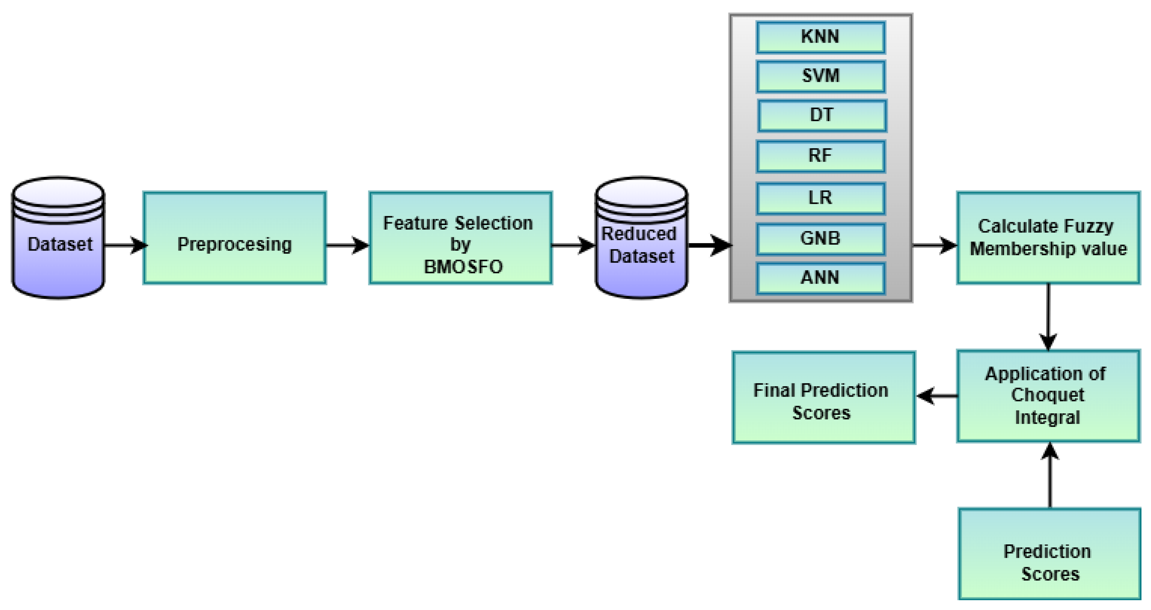
Figure 2.
Population Initialization.
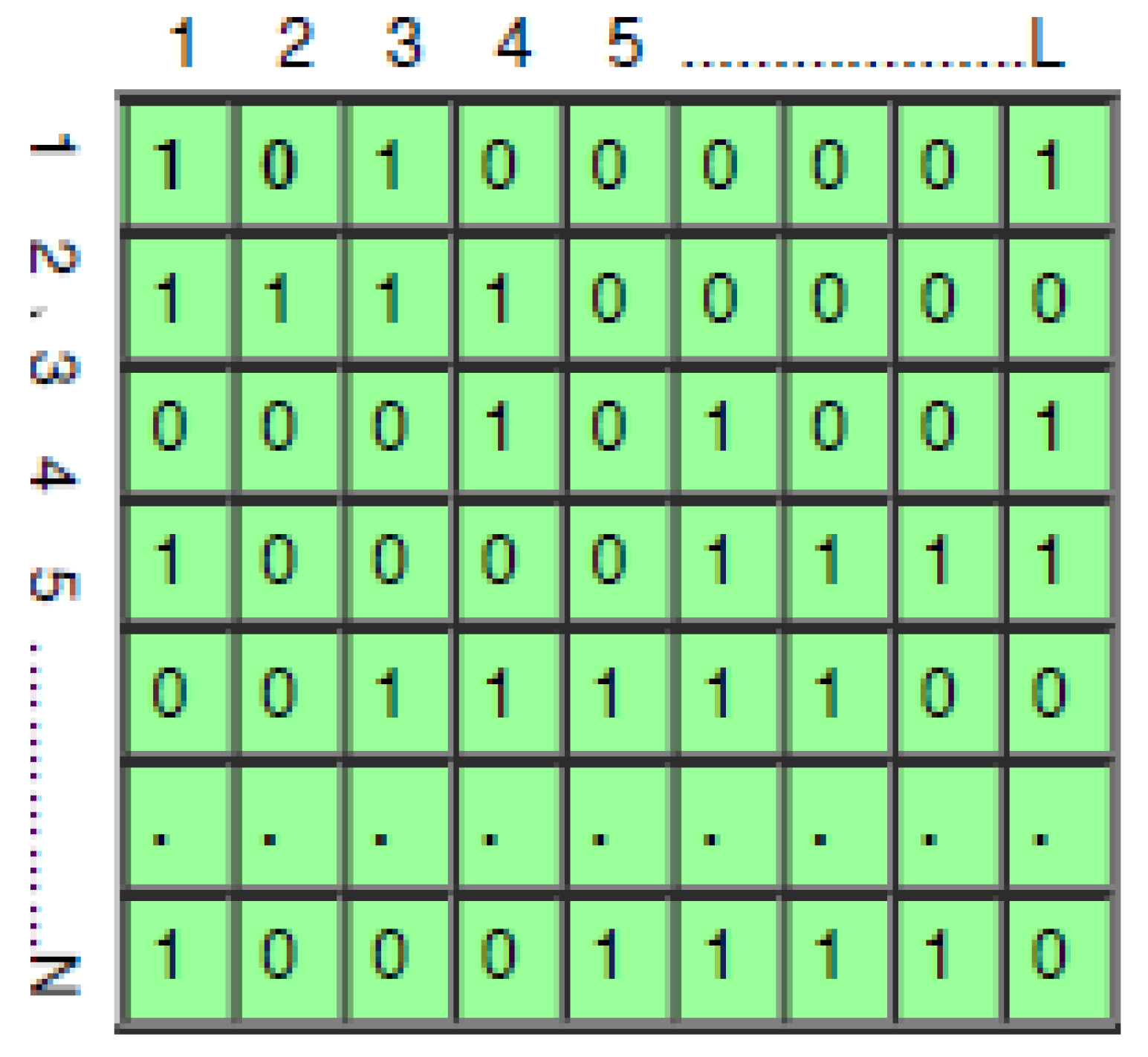
Figure 3.
Starfish Biological Characteristics: (a, b) body structure, (c) reproduction behavior, and (d) prey interaction [45]
Figure 3.
Starfish Biological Characteristics: (a, b) body structure, (c) reproduction behavior, and (d) prey interaction [45]
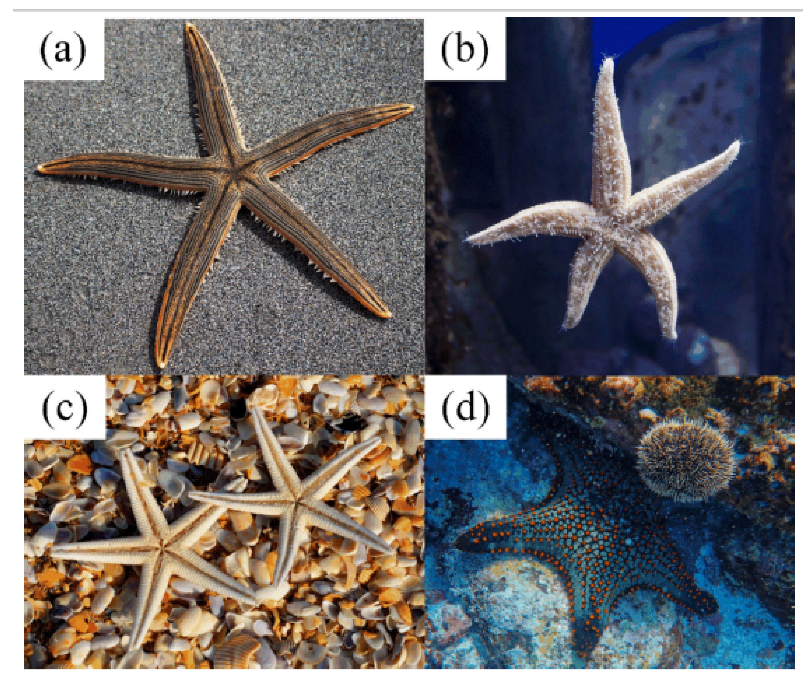
Figure 4.
Workflow of the Proposed BMOSFO for Feature Selection
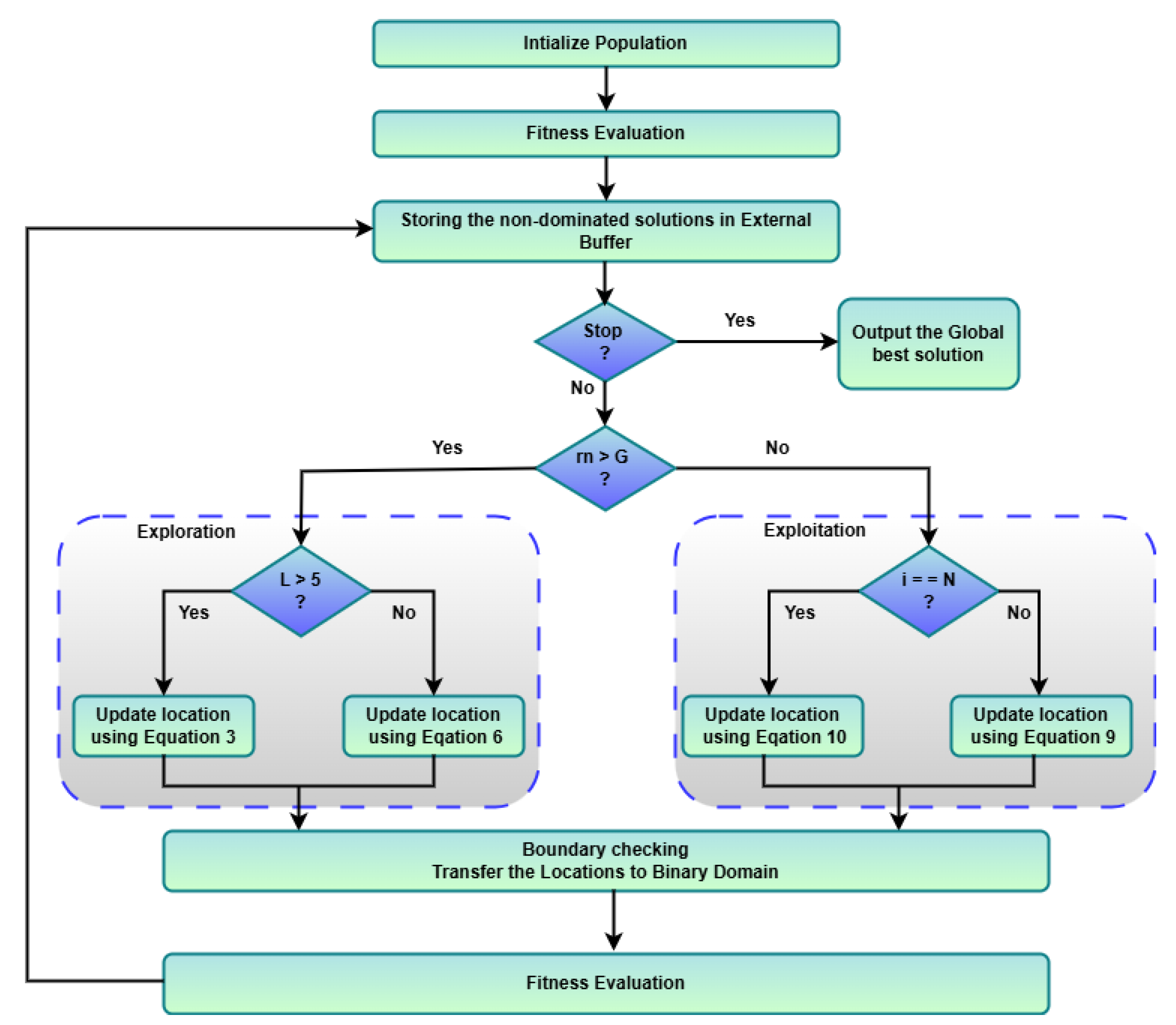
Figure 5.
Pareto Fronts of BMOSFO, MOGA, and MOGWO for Feature Selection.
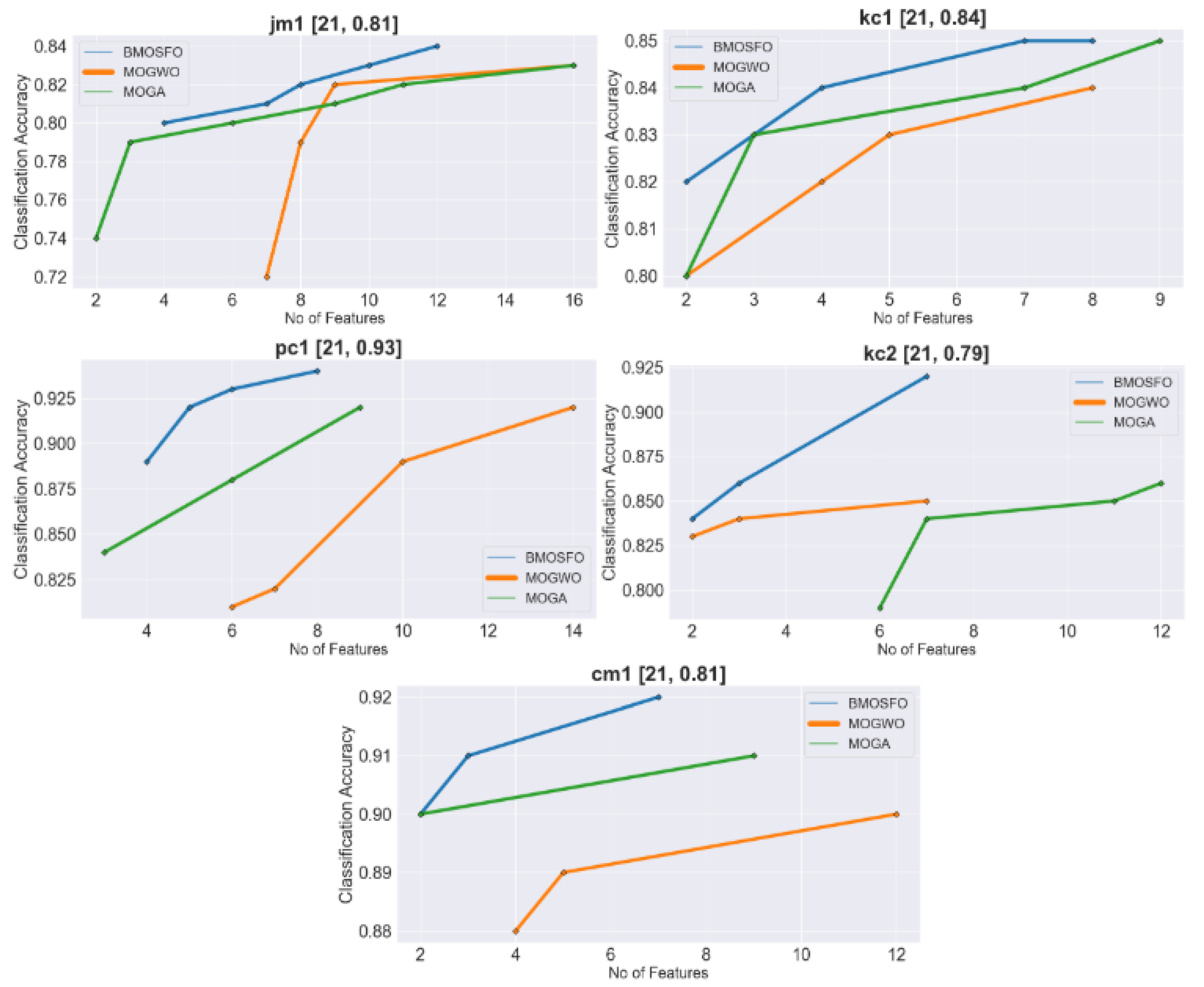
Figure 6.
Impact of Feature Selection on Classification Performance on JM1 Dataset.
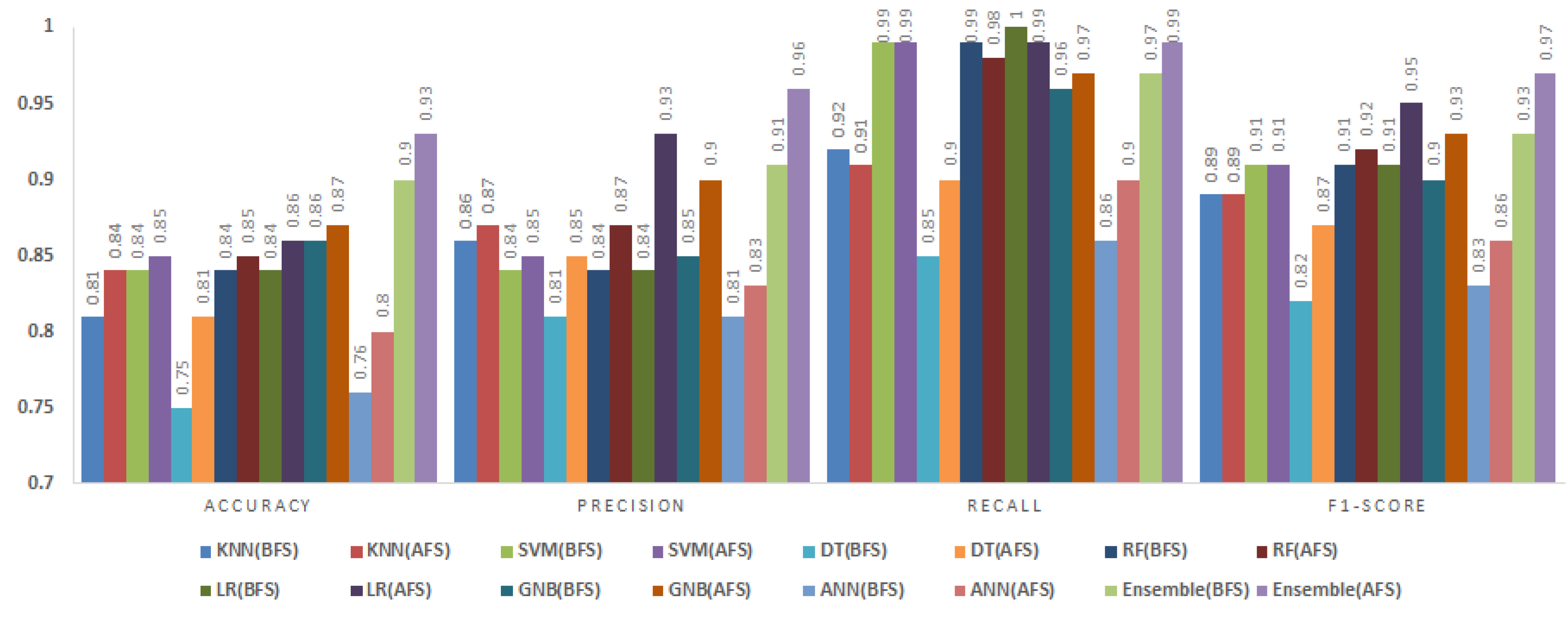
Figure 7.
Impact of Feature Selection on Classification Performance on KC1 Dataset.
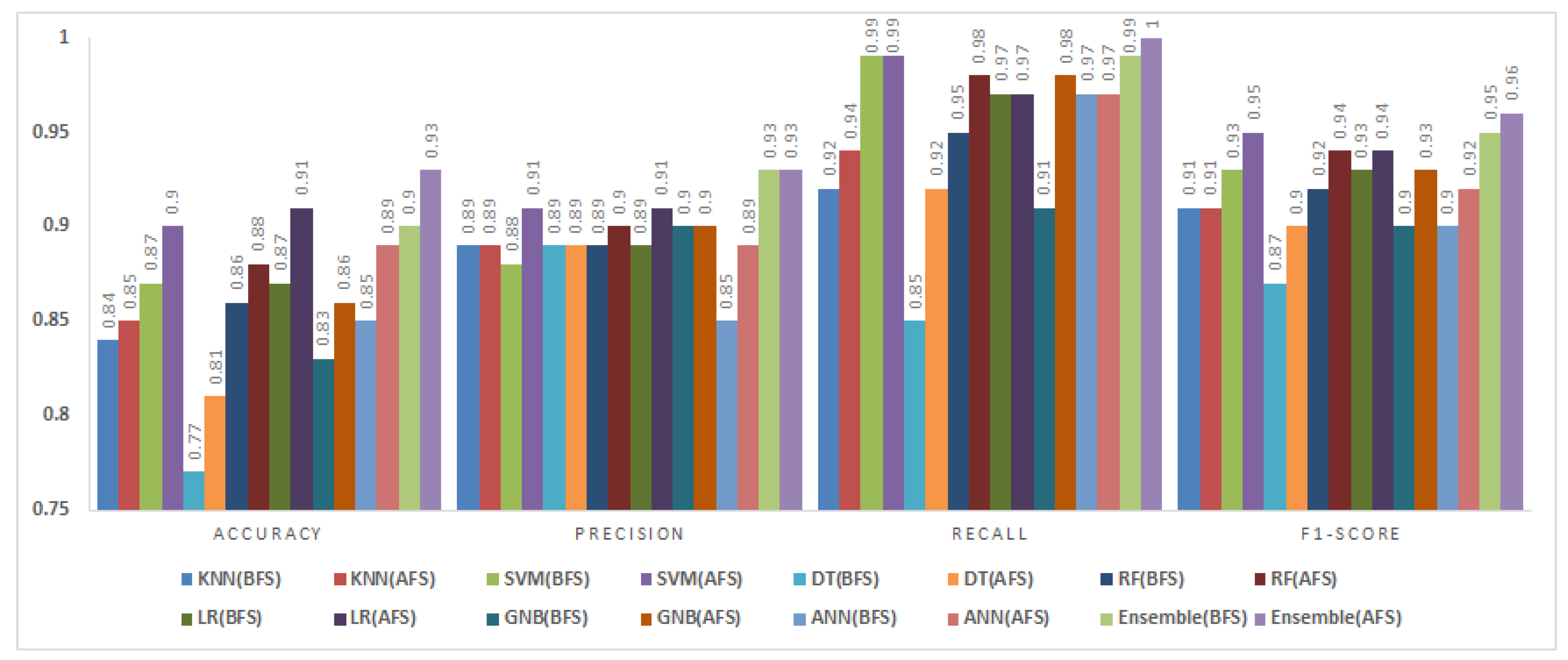
Figure 8.
Impact of Feature Selection on Classification Performance on PC1 Dataset.
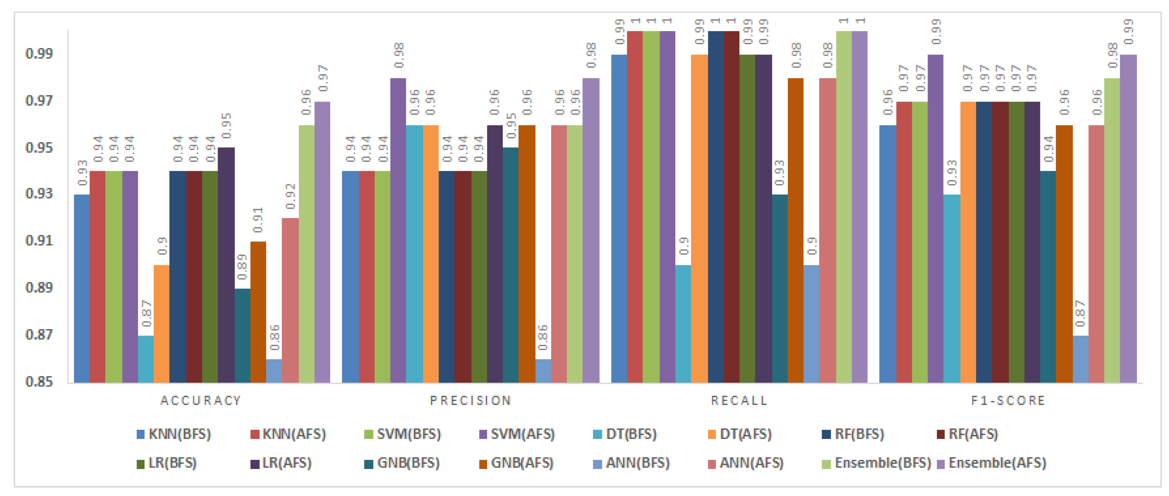
Figure 9.
Impact of Feature Selection on Classification Performance on KC2 Dataset.
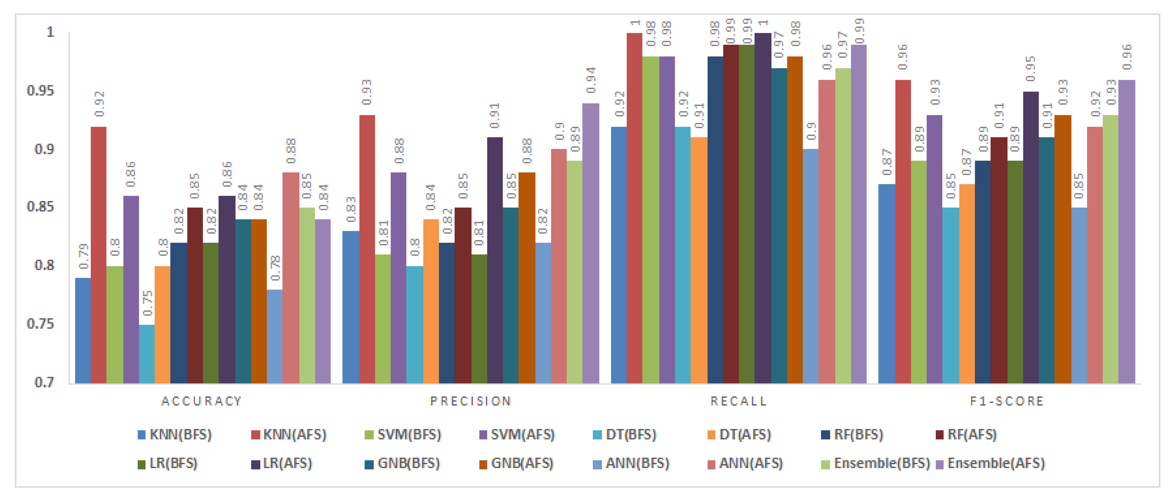
Figure 10.
Impact of Feature Selection on Classification Performance on CM1 Dataset.
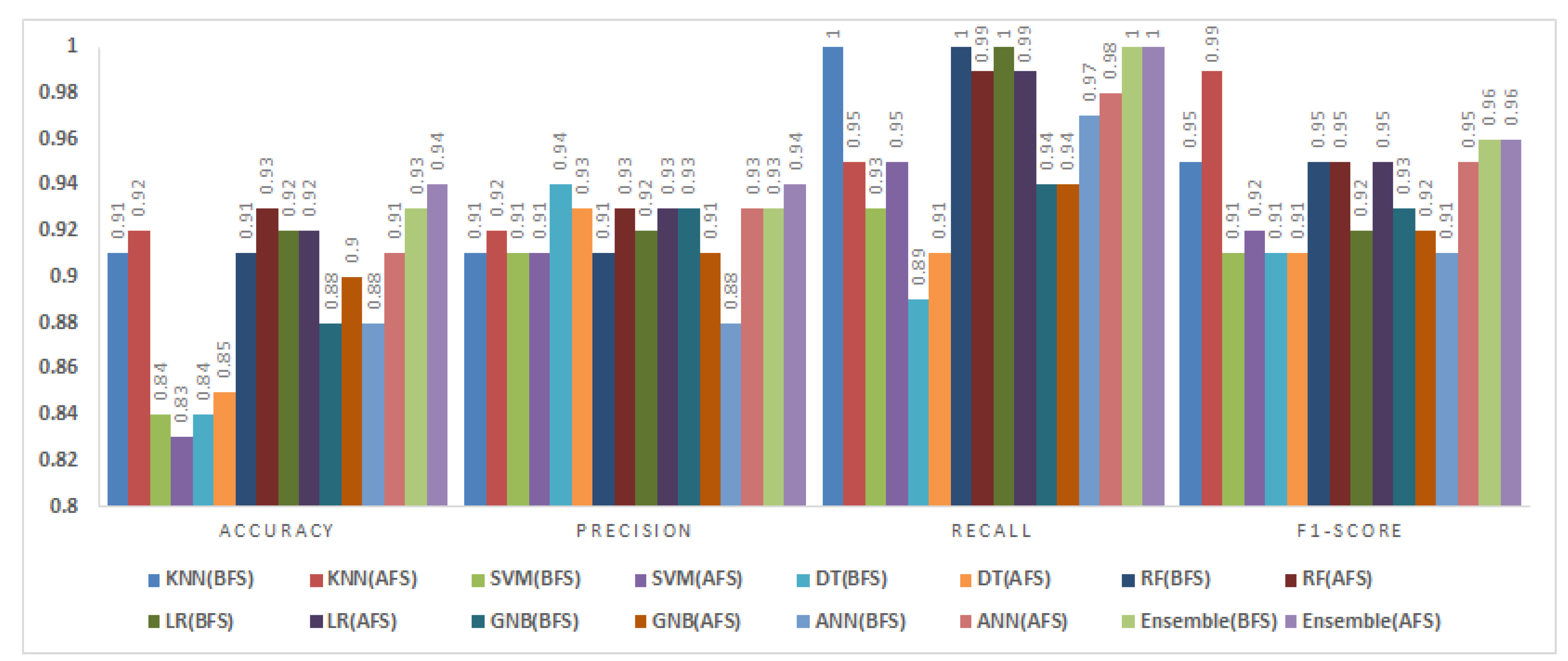

Table 1.
Description of NASA Datasets.
| Dataset | Programming Language | #Modules | % Defected Models | Description |
|---|---|---|---|---|
| JM1 | C | 13,204 | 16% | Software written in C, using Halstead and McCabe metrics for defect prediction. |
| KC1 | C++ | 2,109 | 15.4% | Storage management software handling ground data. |
| PC1 | C | 1,109 | 6.8% | Flight software from an earth-orbiting satellite. |
| KC2 | C++ | 522 | 20% | Science data processing software. |
| CM1 | C | 498 | 9.7% | NASA spacecraft instrument data processing. |
Table 2.
Features Present in NASA Datasets.
| SNO | Features | |
|---|---|---|
| 1 | McCabe Metrics | Line count of code |
| 2 | Cyclomatic complexity | |
| 3 | Essential complexity | |
| 4 | Design complexity | |
| 5 | Halstead Metrics | Total operators + operands |
| 6 | Volume | |
| 7 | Program length | |
| 8 | Difficulty | |
| 9 | Intelligence | |
| 10 | Effort | |
| 11 | Number of Delivered Bugs | |
| 12 | Time estimator | |
| 13 | Line count | |
| 14 | Count of lines of comments | |
| 15 | Count of blank lines | |
| 16 | Lines containing both code and comments | |
| 17 | Unique operators | |
| 18 | Unique operands | |
| 19 | Total operators | |
| 20 | Total operands | |
| 21 | Branch count of the flow graph | |
| 22 | Number of defects | |
Table 3.
Parameter Settings for Feature Selection Algorithms.
| Parameters | BMOSFO | MOGA | MOGWO |
|---|---|---|---|
| Iterations | 50 | 50 | 50 |
| Population Size | 100 | 100 | 100 |
| Repository Size | 50 | 50 | 50 |
| Crossover Rate | N/A | 0.8 | N/A |
| Mutation Rate | N/A | 0.05 | N/A |
Table 4.
Performance Metrics of Classifiers on JM1 Dataset Before Feature Selection.
| Classifiers | Accuracy | Precision | Recall | F1-Score |
|---|---|---|---|---|
| KNN | 0.81 | 0.86 | 0.92 | 0.89 |
| SVM | 0.84 | 0.84 | 0.99 | 0.91 |
| DT | 0.75 | 0.81 | 0.85 | 0.82 |
| RF | 0.84 | 0.84 | 0.99 | 0.91 |
| LR | 0.84 | 0.84 | 1.00 | 0.91 |
| GNB | 0.83 | 0.85 | 0.96 | 0.90 |
| ANN | 0.76 | 0.81 | 0.86 | 0.83 |
| Fuzzy Ensemble | 0.90 | 0.91 | 0.97 | 0.93 |
Table 5.
Performance Metrics of Classifiers on KC1 Dataset Before Feature Selection.
| Classifiers | Accuracy | Precision | Recall | F1-Score |
|---|---|---|---|---|
| KNN | 0.84 | 0.89 | 0.92 | 0.91 |
| SVM | 0.87 | 0.88 | 0.99 | 0.93 |
| DT | 0.77 | 0.89 | 0.85 | 0.87 |
| RF | 0.86 | 0.89 | 0.95 | 0.92 |
| LR | 0.87 | 0.89 | 0.97 | 0.93 |
| GNB | 0.83 | 0.90 | 0.91 | 0.90 |
| ANN | 0.85 | 0.85 | 0.97 | 0.90 |
| Fuzzy Ensemble | 0.90 | 0.93 | 0.99 | 0.95 |
Table 6.
Performance Metrics of Classifiers on PC1 Dataset Before Feature Selection.
| Classifiers | Accuracy | Precision | Recall | F1-Score |
|---|---|---|---|---|
| KNN | 0.93 | 0.94 | 0.99 | 0.96 |
| SVM | 0.94 | 0.94 | 1 | 0.97 |
| DT | 0.87 | 0.96 | 0.90 | 0.93 |
| RF | 0.94 | 0.94 | 1 | 0.97 |
| LR | 0.94 | 0.94 | 0.99 | 0.97 |
| GNB | 0.89 | 0.95 | 0.93 | 0.94 |
| ANN | 0.86 | 0.86 | 0.90 | 0.87 |
| Fuzzy Ensemble | 0.96 | 0.96 | 1 | 0.98 |
Table 7.
Performance Metrics of Classifiers on KC2 Dataset Before Feature Selection.
| Classifiers | Accuracy | Precision | Recall | F1-Score |
|---|---|---|---|---|
| KNN | 0.79 | 0.83 | 0.92 | 0.87 |
| SVM | 0.80 | 0.81 | 0.98 | 0.89 |
| DT | 0.75 | 0.80 | 0.92 | 0.85 |
| RF | 0.82 | 0.82 | 0.98 | 0.89 |
| LR | 0.82 | 0.81 | 0.99 | 0.89 |
| GNB | 0.84 | 0.85 | 0.97 | 0.91 |
| ANN | 0.78 | 0.82 | 0.90 | 0.85 |
| Fuzzy Ensemble | 0.85 | 0.89 | 0.97 | 0.93 |
Table 8.
Performance Metrics of Classifiers on CM1 Dataset Before Feature Selection.
| Classifiers | Accuracy | Precision | Recall | F1-Score |
|---|---|---|---|---|
| KNN | 0.91 | 0.91 | 1 | 0.95 |
| SVM | 0.84 | 0.91 | 0.93 | 0.91 |
| DT | 0.84 | 0.94 | 0.89 | 0.91 |
| RF | 0.91 | 0.91 | 1 | 0.95 |
| LR | 0.92 | 0.92 | 1.00 | 0.92 |
| GNB | 0.88 | 0.93 | 0.94 | 0.93 |
| ANN | 0.88 | 0.88 | 0.97 | 0.91 |
| Fuzzy Ensemble | 0.93 | 0.93 | 1 | 0.96 |
Table 9.
HyperVolume Values of Pareto Fronts for Feature Selection.
| Datasets | MOGA | MOGWO | BMOSFO |
|---|---|---|---|
| JM1 | 0.21 | 0.28 | 0.30 |
| KC1 | 0.29 | 0.22 | 0.37 |
| PC1 | 0.28 | 0.19 | 0.40 |
| KC2 | 0.20 | 0.22 | 0.34 |
| CM1 | 0.17 | 0.22 | 0.36 |
Table 10.
Number of Selected Features vs. Classification Accuracy.
| Datasets | MOGA | MOGWO | BMOSFO |
|---|---|---|---|
| JM1 | [16, 0.83] | [16, 0.83] | [12, 0.84] |
| KC1 | [9, 0.85] | [8, 0.84] | [7, 0.85] |
| PC1 | [3, 0.84] | [14, 0.92] | [8, 0.94] |
| KC2 | [6, 0.79] | [7, 0.85] | [7, 0.92] |
| CM1 | [9, 0.91] | [12, 0.90] | [7, 0.92] |
Table 11.
Selected Features by BMOSFO for Each Dataset.
| Dataset | Selected Features |
|---|---|
| JM1 | Cyclomatic complexity, Essential complexity, Operators + Operands (McCabe), volume, difficulty, Time to write program, Line count, Count of lines of comments Count of blank lines, unique operands (Halstead), Total operators, Number of branches in flow graph |
| KC1 | Halstead total Operators + Operands, McCabe Design Complexity, Branch Count, total Operand, McCabe Design Complexity, Halstead Program Length, Number of Unique operators |
| PC1 | McCabe “design complexity”, Halstead “difficulty”, Branch Count, Halstead “Number of Delivered Bugs”, Halstead’s time estimator: time to write a program, Total Number of operators + operands, McCabe Design Complexity, Halstead Program Length |
| KC2 | McCabe “design complexity”, Operators + Operands, volume, Halstead “difficulty”, Effort: Halstead effort to write program, Halstead’s time estimator: time to write a program, Count of lines which contain both code and comments |
| CM1 | McCabe "cyclomatic complexity”, McCabe "essential complexity”, McCabe "design complexity”, Halstead "program length”, Halstead "difficulty”, Halstead’s line count, branchCount of the flow graph |
Disclaimer/Publisher’s Note: The statements, opinions and data contained in all publications are solely those of the individual author(s) and contributor(s) and not of MDPI and/or the editor(s). MDPI and/or the editor(s) disclaim responsibility for any injury to people or property resulting from any ideas, methods, instructions or products referred to in the content. |
© 2025 by the authors. Licensee MDPI, Basel, Switzerland. This article is an open access article distributed under the terms and conditions of the Creative Commons Attribution (CC BY) license (http://creativecommons.org/licenses/by/4.0/).
Copyright: This open access article is published under a Creative Commons CC BY 4.0 license, which permit the free download, distribution, and reuse, provided that the author and preprint are cited in any reuse.


