
Submitted:
28 February 2025
Posted:
04 March 2025
You are already at the latest version
Abstract
In this paper, we introduce the Bayesian Gibbs Slice Sampler (BGSS), a novel MCMC algorithm inspired in the Latent Slice Sampling (LSS) framework, where Bayesian inference is employed to refine the proposal distribution required to accommodate the single adjustment parameter. Unlike methods based on gradient calculations or those requiring complex, hard-to-optimize adaptive proposals, BGSS naturally incorporates Bayes’ theorem during the chain adaptation phase to learn about the target distribution. Subsequently, it generates nearly independent proposals derived from a conditionally univariate factorization of the parameter space, along with a QR decomposition, thus conferring substantial efficiency to the exploration process. The proposed sampler is both adaptable and computationally effective, matching the speed of LSS and delivering results on par with state-of-the-art approaches like the No-U-Turn Sampler (NUTS). We display its capabilities through simulated and real-world applications, highlighting an analysis of sovereign credit ratings and illustrating how BGSS can model the influence of macroeconomic fundamentals over multiple time horizons. Overall, BGSS strikes a favourable balance between performance and computational demands, making it a dependable tool for Bayesian inference in econometric contexts.
Keywords:
Bayesian Methods
; MCMC
; Slice Sampling
; Sovereign Risk
1. Introduction
In the Bayesian inferential framework, the calculation of the posterior distribution of the parameters of a model constitutes a primary objective. However, it is frequently observed that posterior densities are not analytically tractable, thus requiring the employment of numerical methods for their approximate calculation. Among these methodologies, Markov Chain Monte Carlo (MCMC) techniques have been the most extensively used due to their exactness and relative ease of application. Nevertheless, these techniques may exhibit convergence issues within chains or require substantial computational time to achieve reliable exploration.
At present, one of the most frequently applied methods for posterior estimation is the No-U-Turn Sampler (NUTS) (Hoffman & Gelman, 2014), which explores densities using Hamiltonian equations and facilitates the automatic adjustment of parameters required in the sampling process. However, this method, along with others that rely on the aforementioned Hamiltonian equations of motion (Neal, 2011; Girolami & Calderhead, 2011), demands analytical or approximate knowledge of the gradient of the posterior density. This requirement can be disadvantageous when time is a critical resource.
An efficient alternative, albeit complex to implement except in isolated cases, is Slice Sampling (Damlen et al., 1999; Neal, 2003). The fundamental principle of Slice Sampling involves introducing an auxiliary variable to transform the problem of sampling from a one-dimensional distribution into sampling from a region or "slice" of the distribution. This approach enables expeditious exploration of the posterior distribution, eliminating the necessity for a rejection step, as in Metropolis-Hastings (Hastings, 1970), and exhibits notable convergence properties (Roberts & Rosenthal, 1999; Mira & Tierney, 2002). However, determining the region or "slice" is often infeasible, requiring the use of approximation methods. In addition to the limitation posed by the general scheme in systematically identifying the slice region, multivariate slice sampling also encounters efficiency issues when the parameter space is high-dimensional or highly correlated.
In light of the previously mentioned aspects of Slice Sampling, researchers have devoted substantial attention to tackling, or at least partially alleviating, its inherent constraints. Some of the most notable contributions, to the best of our knowledge, are the papers of Murray et al. (2010), Murray & Adams (2010), Tibbits et al. ( 2014), Karamanis & Beutler (2021). Li & Walker (2023) or Schär et al. (2023). Notwithstanding these advancements, we posit that remains potential for further improvement in this area. Concretely, this paper presents a novel methodology that obviates the necessity for gradient computation, while preserving efficiency throughout the exploration phase. The proposed sampling framework demonstrates a capability to explore the parameter space with comparable speed to other well-established algorithms.
The structure of this paper is organized as follows. Section 2 develops the proposed algorithm. Section 3 presents a simulated scenario in which we compare the performance of our method against some of the principal samplers widely utilized. In Section 4, we estimate a panel data model wherein the short-term and long-term effects of certain macroeconomic fundamentals on sovereign credit ratings are quantified. Finally, in Section 5, we conclude with a discussion of the primary results obtained and propose several resulting lines of research that emerge from this work.
2. Bayesian Gibbs Slice Sampler
Consider a dataset consisting of a target variable and an associated set of explanatory variables , where represents the number of observations and the number of explanatory variables. Each observation is linked to a row vector , representing the explanatory information relevant for understanding the underlying data-generating process.
To describe this relationship, we specify a stochastic model with parameter vector . We adopt a Bayesian approach by incorporating prior beliefs about through a prior distribution . By applying Bayes’ theorem, we update our information about in light of the observed data :
where is the marginal distribution of y. The posterior distribution encapsulates all information about after the data have been observed, effectively blending prior assumptions with empirical evidence. Henceforth, we shall refer to the proportional quantity in (2.1) as the posterior kernel, following Geweke (2005). Typically, this distribution is not analytically tractable and must be calculated using approximation methods, usually Monte Carlo Markov Chain (MCMC) methods.
2.1. Slice sampling
In the standard univariate slice sampling scheme, the target distribution is . The algorithm introduces a latent variable , where represents the iteration of the chain, and draws from a uniform distribution, which effectively "slices" the posterior distribution at the level . This slicing defines the set , representing the region of parameter values where the posterior density exceeds the slice level. Subsequently, a new sample is drawn uniformly from the set , i.e., . By iterating this process from to , the algorithm generates a sequence of samples that, under appropriate conditions (Mira & Tierney, 2002), converges to the target posterior distribution . This method facilitates efficient exploration of the parameter space without the need for additional accept-reject steps. Assuming is one-dimensional, the Slice Sampling algorithm proceeds as follows:
| Univariate Slice Sampling | |
| Input: A random value | |
| Output: A sequence of samples from a target posterior distribution. | |
| From to , repeat: | |
| 1. | ; where is a latent variable used to “slice” the target, and represents a Uniform continuous distribution. |
| 2. | where is a bound defined by the current “slice”. |
Primary challenges associated with simple Slice Sampling are twofold. On one hand, determining the set on each iteration can be difficult even in one-dimensional cases. The other issue, shared by other widely accepted MCMC schemes such as Metropolis-Hastings, is the random walk exploration in multivariate cases. We refer to random walk behaviour as a chain that tends to move slowly through the parameter space, resulting in inefficient exploration. Such behaviour leads to poor mixing and increased autocorrelation among samples. This, in turn, hinders the chain’s ability to converge rapidly to the target distribution, ultimately undermining the overall efficiency of the MCMC procedure.
We first put the focus on how determining . Neal (2003) introduces two procedures, stepping-out and doubling. This involves defining some quantities , where and represent the lower and upper boundaries, respectively, that define the sampling interval over which the marginal posterior density of is defined by the current slice. In other words, the sampling intervals refer to the region over the parameter space for which the posterior density remains above a certain threshold . The stepping-out method incrementally expands this sampling interval starting from an initial point. It begins by placing and for close to the starting position and then progressively "steps out" in both directions by a fixed step size until the entire region where is likely contained. Each time the step extends the interval, the algorithm checks whether the current bounds and ; for still enclose a region meeting the density threshold. This iterative expansion continues until no further extension is needed, ensuring that the final covers all acceptable values.
The doubling procedure, on the other hand, employs a more aggressive strategy to determine the sampling interval. Instead of stepping out incrementally, it rapidly expands the interval by repeatedly doubling its size around the initial point. After each doubling, it checks whether the newly expanded interval encompasses the full slice of interest. This process continues until is fully contained. Because doubling can quickly overshoot, this approach requires a reversibility condition: once the interval is large enough, the algorithm may need to contract it in a controlled manner to ensure that the final interval accurately reflects the high-probability region without excluding relevant areas or including irrelevant ones.
In both the stepping-out and doubling cases, reaching an optimal interval that accurately reflects the slice often requires multiple evaluations of the target function . The methods rely on iterative updates and density checks to ensure that the sampling interval correctly encompasses the desired high-likelihood region, ultimately improving the efficiency and accuracy of slice sampling in Bayesian inference.
2.2. Latent Slice Sampling
An innovative enhancement to address the challenge of continuous evaluation in slice sampling is the Latent Slice Sampler (LSS), introduced by Li and Walker (2023). LSS establishes the initial set randomly in each iteration by leveraging a new latent variable . Specifically, is drawn from a uniform distribution defined as , where ; . The latent variable serves as a midpoint within the interval , ensuring that the newly established interval limits and encapsulate a point within the posterior distribution. This mechanism guarantees that the sampling interval is centered around a region of high posterior density, thereby enhancing the efficiency of the exploration process.
Furthermore, LSS introduces a probability density function , univariate but the same for all j, which serves to determine randomly the width of the sampling interval at each iteration. Individually, the function is designed to generate random samples for in a way that satisfies the condition . This condition ensures that the interval remains appropriately sized relative to the distance between the current parameter value and the latent midpoint . To achieve this, must be carefully tuned to balance the exploration breadth and the acceptance rate of the proposed samples. In their work, Li and Walker (2023) propose in various examples using a Gamma distribution, specifically , where denotes the Gamma distribution and is a shape parameter that controls the distribution's scale. We will follow this convention in the rest of the paper. Selecting an appropriate is critical; while favourable outcomes are observed with low values of in several examples, empirical applications may require fine-tuning to accommodate specific data characteristics, as discussed in Section 4. The primary trade-off of this approach lies in the necessity of tuning the density function , which can be non-trivial in practice. Additionally, LSS does not address the issue of random walk behavior in multivariate settings, limiting its applicability in high-dimensional parameter spaces. To illustrate the LSS process, we present the univariate version as pseudocode, to alleviate the notational charge:
| Latent Univariate Slice Sampling | |
| Input: A random value , a value and a probability density function to draw random samples from | |
| Output: A sequence of samples from the target posterior distribution. | |
| From to , repeat steps 1 to 5: | |
| 1. | Draw |
| 2. | Draw |
| 3. | Draw a random sample , where is a distribution to be tuned. While ; otherwise the lower () and upper () bounds of are stablished as: |
| 4. | Draw . If ; else if ; otherwise . Repeat step 4 while . |
| 5. | Set |
The primary advantage of the LSS algorithm is its execution speed, which is significantly faster compared to other MCMC methods. This efficiency stems from the algorithm's ability to dynamically adjust the sampling interval based on the latent midpoint and the interval width , thereby reducing the need for extensive evaluations of the posterior density. However, this efficiency comes with the trade-off of requiring careful tuning of the density function . Selecting an appropriate for the Gamma distribution is essential to ensure that the condition is satisfied consistently, which can be challenging in empirical applications as elaborated in Section 4. Additionally, LSS does not address the issue of random walk behavior in multivariate scenarios, which can lead to inefficient exploration in high-dimensional parameter spaces.
2.3. Proposed algorithm: Bayesian Gibbs Slice Sampler
The proposed Bayesian Gibbs Slice Sampler (BGSS) adopts a stochastic approach analogous to the Latent Slice Sampler (LSS) for defining the set . However, BGSS does not employ a latent variable to find a midpoint, eliminates the need to tune any proposal distribution and facilitates efficient exploration of a multivariate parameter space, thereby mitigating the random walk behaviour typically encountered in traditional MCMC methods. We delineate each improvement step systematically. The principal innovation of BGSS lies in leveraging Bayes' theorem to define the set during the adaptation phase, a novel approach not extensively covered in existing literature, at least to our knowledge.
2.3.1. Baye’s Theorem to approximate the set A
Again, let be a random vector where each component is defined as . As each needs to be defined over a positive support, we assume that follows a log normal distribution:
where and representing the mean and variance of , respectively. This distribution is employed in each iteration to determine an approximation to for each individually. During each iteration of the chain, a new sample is drawn from the updated predictive density, in order to take into account the information contained in the posterior of , generating a sequence , which defines a likelihood function:
Here, denotes the current iteration, and the sequence is terminated once , where marks the end of the burn-in period. Essentially, the burn-in phase is utilized to calibrate the random vector , which stochastically defines individually an initial set within the Slice Sampling framework. Unlike LSS, which employs a latent variable, BGSS makes use of Bayes Theorem to define the quantity randomly. In brief, our proposal involves adding, at each new iteration of the Markov chain, an element obtained after completing a Slice Sampling iteration, thereby defining a sequence that provides information on the different states of encountered during the burn-in period. By applying Bayes’ Theorem, we incorporate all available prior information about the parameters that define the likelihood of the sequence and then establish a posterior density for these parameters. Finally, from the conditional posterior densities, which have known forms, a point estimate for the parameters shaping the likelihood is extracted and used to obtain a random sample from the predictive density of a new element, employing the mean of a set of Monte Carlo samples. To sample from the predictive distribution, we must infer new values for the parameters and on each iteration. This is achieved through Bayesian inference by defining the posterior distribution via Bayes' theorem:
where is the prior distribution of . This method provides a benefit compared to heuristic or optimization-based approaches by allowing any existing information about to be systematically incorporated into the model. We adopt Jeffreys' objective prior for , reflecting complete prior ignorance about the true parameter values:
as proposed by (Jeffreys, 1961). This choice of prior, combined with the likelihood function , facilitates the derivation of the posterior conditional distributions necessary for inferring and at each iteration. The joint posterior is then used to derive the posterior predictive distribution for a new value from:
where , and denotes a t-Student distribution. Therefore, a new sample for can be drawn as . See Appendix A for further details.
2.3.2. QR Decomposition
While not essential for the core functionality of BGSS, QR decomposition can be employed to reduce correlations among parameters, thereby facilitating more efficient exploration of the parameter space. To apply the QR decomposition on , we must find a suitable pair of matrixes such , where is an orthogonal matrix, and an upper-triangular matrix. To weight both matrix in terms of sample size, we opt to define equivalently and . Under this transformation, we substitute:
and employ on sampling:
where . After completing each iteration, and for returning the real value of , we just simply obtain the inverse . In the user’s guide of STAN programming language (Carpenter et al., 2017), the reader can find more information about QR decomposition and how to apply it on different frameworks.
2.3.3. Gibbs-sampling scheme
Now we put the focus on the issue of random walk behaviour in multivariate settings. Existing alternatives leveraging the slice sampling scheme include the Factor Slice Sampler (Tibbits et al., 2014), which utilizes a rotated orthogonal basis for efficient exploration, and the Ensemble Slice Sampler (Karamanis & Beutler, 2021), which employs parallel chains, or "walkers," to achieve affine-invariant transformations (Goodman & Weare, 2010). Our proposal in this regard is to incorporate a Gibbs sampling–type scheme along with the QR decomposition. This combination of schemes is necessary because, on their own, they do not alleviate the random walk problem. In initial simulations, it was observed that using the QR transformation in isolation, without employing a Gibbs-type update, improved the chain’s convergence but ultimately proved insufficient to achieve the goal. This is because although the QR transformation reorients the parameter space and reduces inter-parameter correlations, it does not directly tackle the inherent inefficiencies of updating parameters as a block. Without sequential conditioning, the updates still suffer from high variance and lack of adaptivity to local features of the target distribution. Similarly, when the performance of updating the parameters conditionally was analysed, convergence improved compared to a block update like the original Slice Sampling proposals, yet once again, it proved inadequate. This occurs because while conditional updates via the Gibbs scheme efficiently reduce variance—by exploiting the Rao–Blackwell effect—and capture local dependencies, they alone cannot fully overcome the challenges posed by a poorly structured parameter space. Only when these conditional updates are combined with the QR transformation, which effectively reparameterizes the space to diminish problematic correlations, do the two techniques synergize to mitigate random walk behaviour and achieve substantial efficiency gains. In essence, the QR transformation and the Gibbs-type update address different facets of the sampling challenge: the former restructures the geometry of the parameter space to enhance mixing, while the latter refines the sampling process by reducing variance and adapting to local characteristics. Together, they form a complementary strategy that is significantly more effective than either approach in isolation.
Therefore, the transition kernel from under our proposition would be:
2.3.4. Full proposal
Given the previous innovations, a pseudocode for Multivariate Bayesian Gibbs Slice Sampling is provided:
| Multivariate Bayesian Gibbs Slice Sampling | |
| Input: A set of random values , , . | |
| Output: A sequence of samples from a target posterior distribution. | |
| From to , repeat: | |
| 1 |
Adaptation during burn-in: While Set , where Set , being Else: Set and |
| 2 |
Draw a new slice: Draw |
| 3 |
Sampling Interval determination: Draw a new value |
| 4 |
Interval construction: Set and , |
| 5 |
Parameter update: For : Draw . If , else: If , otherwise . Repeat while . |
| 6 |
Update Sampling Interval: For : Set |
As a final remark, it is worth noting that no additional criteria have been adopted regarding the choice of the calibration period , nor for the number of samples to draw in order to define the new value of . In the various simulation exercises and empirical applications described in this paper, the initial 20% of the sample was discarded as burn-in, and 50 random samples were drawn from the likelihood, conditioned on the new posterior parameter estimates. This choice has worked satisfactorily in all the challenges presented, although we remain open to exploring methods that allow for a less heuristic definition of both values.
3. Simulation Study
In this section we analyse the performance of our proposal and compare it in terms of efficiency and computational time against the LSS sampler, with different choices of tunning for , and NUTS. All programs created for this paper are based on Julia Programming Language, (Bezanson et al., 2017), using Turing.jl, (Ge et al., 2018), to conduct posterior simulation for LSS and NUTS. We propose analyse the following dynamic regression model:
that describes the evolution of the variable of interest , according to its first lag, a set of exogenous explanatory variables with K = 10 and are i.i.d. homoscedastic random normal disturbances, with and . We take:
The explanatory variables have been created as a multivariate gaussians following the specification:
where, and is the maximum eigenvalue of , needed to control condition number.
Three simulation scenarios have been proposed, which differ only in the sample size used. We consider a small sample size, , a medium sample size , and a big sample . We also define the next prior distributions:
being the notation for an Inverse Gamma distribution. The associated posterior kernel is:
We run 5 parallel chains of iterations per chain, and a warm-up of iterations, also, per chain. The statistics used to report the results include the posterior mean (Mean), the posterior standard deviation (SD), the 2.5th percentile (Q. 2.5), the median or 50th percentile (Q. 50), and the 97.5th percentile (Q. 97.5). Additionally, the convergence measures, ESS and , are used to evaluate the convergence of the chains and the quality of the results. Notice that represents the potential scale-reduction factor, and ESS is the Effective ample Size, which are both defined in (Gelman et al. 2014). The proposal distributions in LSS are , where we assing three different values for , , and , respectively. Our analysis begins with a comparison of BGSS performance against the benchmarked LSS proposals, followed by a focused examination of NUTS. Regarding BGSS against LSS, results are provided in Table 3.1 to 3.6:

Table 3.1.
Posterior results. T = 50. BGSS vs LSS.
| Variable | Mean | SD | ESS | |||||||||||||||||||
|---|---|---|---|---|---|---|---|---|---|---|---|---|---|---|---|---|---|---|---|---|---|---|
| True | (1) | (2) | (3) | (4) | (1) | (2) | (3) | (4) | (1) | (2) | (3) | (4) | (1) | (2) | (3) | (4) | ||||||
| σ² | 1.0000 | 1.0591 | 1.0083 | 1.0267 | 1.0464 | 0.4150 | 0.2347 | 0.2428 | 0.2500 | 13452 | 474 | 440 | 273 | 1.0001 | 1.0015 | 1.0176 | 1.0058 | |||||
| ρ | 0.7500 | 0.7289 | 0.7382 | 0.7380 | 0.7382 | 0.0239 | 0.0221 | 0.0224 | 0.0225 | 31405 | 1827 | 1647 | 1915 | 1.0000 | 1.0004 | 1.0026 | 1.0000 | |||||
| β1 | 4.5371 | 4.0272 | 3.9660 | 3.9472 | 3.9395 | 0.1987 | 0.1880 | 0.1907 | 0.1938 | 30579 | 545 | 484 | 327 | 1.0000 | 1.0008 | 1.0109 | 1.0049 | |||||
| β2 | 1.9836 | 2.0234 | 1.8979 | 1.9019 | 1.9008 | 0.2169 | 0.2165 | 0.2157 | 0.2116 | 33451 | 311 | 281 | 231 | 1.0001 | 1.0010 | 1.0085 | 1.0097 | |||||
| β3 | 0.0000 | -0.2703 | -0.2971 | -0.2676 | -0.2504 | 0.2504 | 0.2388 | 0.2294 | 0.2296 | 34588 | 207 | 220 | 201 | 1.0000 | 1.0003 | 1.0014 | 1.0055 | |||||
| β4 | -1.9752 | -2.0386 | -1.9541 | -1.9595 | -1.9697 | 0.2424 | 0.2384 | 0.2370 | 0.2291 | 33837 | 247 | 234 | 261 | 1.0000 | 1.0071 | 1.0102 | 1.0096 | |||||
| β5 | -1.2742 | -1.1382 | -1.0845 | -1.0921 | -1.0864 | 0.1775 | 0.1759 | 0.1823 | 0.1715 | 33376 | 315 | 244 | 304 | 1.0000 | 1.0059 | 1.0027 | 1.0011 | |||||
| β6 | -3.4949 | -3.6744 | -3.5389 | -3.5450 | -3.5334 | 0.2140 | 0.2093 | 0.2210 | 0.1997 | 33624 | 297 | 248 | 253 | 1.0000 | 1.0059 | 1.0162 | 1.0007 | |||||
| β7 | 0.0000 | 0.1559 | 0.0931 | 0.0968 | 0.0858 | 0.2053 | 0.2071 | 0.2105 | 0.2127 | 32895 | 335 | 361 | 303 | 1.0000 | 1.0019 | 1.0012 | 1.0020 | |||||
| β8 | -2.1660 | -2.0134 | -2.0244 | -2.0119 | -2.0076 | 0.2500 | 0.2503 | 0.2499 | 0.2490 | 34480 | 321 | 332 | 230 | 1.0000 | 1.0014 | 1.0001 | 1.0009 | |||||
| β9 | 0.0000 | 0.2084 | 0.2098 | 0.2043 | 0.2130 | 0.1837 | 0.1753 | 0.1825 | 0.1766 | 32690 | 545 | 486 | 319 | 1.0000 | 1.0007 | 1.0013 | 1.0068 | |||||
| β10 | -0.0047 | -0.0077 | -0.0983 | -0.1278 | -0.1428 | 0.2803 | 0.2738 | 0.2744 | 0.2646 | 33485 | 230 | 235 | 204 | 1.0001 | 1.0009 | 1.0040 | 1.0008 | |||||
| (1) refers to BGSS sampling, (2) to LSS (λ = 1), (3) to LSS (λ = 10) and (4) to LSS (λ = 0.1). Real column reflects the real value of each parameter. Mean denotes the marginal posterior mean, SD the Standard Deviation, ESS the Effective Sample Size and represents the potential scale reduction factor. Execution time (in seconds): BGSS = 0.44782, LSS (λ = 1) = 0.782900, LSS (λ = 10) = 0.802070, LSS (λ = 1) = 0.612207. | ||||||||||||||||||||||
Table 3.2.
Posterior quantiles. T = 50. BGSS vs LSS.
| Variable | Q 2.5 | Q 50 | Q 97.5 | ||||||||||||||
|---|---|---|---|---|---|---|---|---|---|---|---|---|---|---|---|---|---|
| True | (1) | (2) | (3) | (4) | (1) | (2) | (3) | (4) | (1) | (2) | (3) | (4) | |||||
| σ² | 1.0000 | 1.0000 | 1.0000 | 1.0000 | 1.0000 | 1.0000 | 1.0000 | 1.0000 | 1.0000 | 1.0000 | 1.0000 | 1.0000 | 1.0000 | 1.0000 | 1.0000 | ||
| ρ | 0.7500 | 0.75 | 0.75 | 0.75 | 0.75 | 0.75 | 0.75 | 0.75 | 0.75 | 0.75 | 0.75 | 0.75 | 0.75 | 0.75 | 0.75 | ||
| β1 | 4.5371 | 4.5371 | 4.5371 | 4.5371 | 4.5371 | 4.5371 | 4.5371 | 4.5371 | 4.5371 | 4.5371 | 4.5371 | 4.5371 | 4.5371 | 4.5371 | 4.5371 | ||
| β2 | 1.9836 | 1.9836 | 1.9836 | 1.9836 | 1.9836 | 1.9836 | 1.9836 | 1.9836 | 1.9836 | 1.9836 | 1.9836 | 1.9836 | 1.9836 | 1.9836 | 1.9836 | ||
| β3 | 0.0000 | 0.0000 | 0.0000 | 0.0000 | 0.0000 | 0.0000 | 0.0000 | 0.0000 | 0.0000 | 0.0000 | 0.0000 | 0.0000 | 0.0000 | 0.0000 | 0.0000 | ||
| β4 | -1.9752 | -1.9752 | -1.9752 | -1.9752 | -1.9752 | -1.9752 | -1.9752 | -1.9752 | -1.9752 | -1.9752 | -1.9752 | -1.9752 | -1.9752 | -1.9752 | -1.9752 | ||
| β5 | -1.2742 | -1.2742 | -1.2742 | -1.2742 | -1.2742 | -1.2742 | -1.2742 | -1.2742 | -1.2742 | -1.2742 | -1.2742 | -1.2742 | -1.2742 | -1.2742 | -1.2742 | ||
| β6 | -3.4949 | -3.4949 | -3.4949 | -3.4949 | -3.4949 | -3.4949 | -3.4949 | -3.4949 | -3.4949 | -3.4949 | -3.4949 | -3.4949 | -3.4949 | -3.4949 | -3.4949 | ||
| β7 | 0.0000 | 0.0000 | 0.0000 | 0.0000 | 0.0000 | 0.0000 | 0.0000 | 0.0000 | 0.0000 | 0.0000 | 0.0000 | 0.0000 | 0.0000 | 0.0000 | 0.0000 | ||
| β8 | -2.1660 | -2.1660 | -2.1660 | -2.1660 | -2.1660 | -2.1660 | -2.1660 | -2.1660 | -2.1660 | -2.1660 | -2.1660 | -2.1660 | -2.1660 | -2.1660 | -2.1660 | ||
| β9 | 0.0000 | 0.0000 | 0.0000 | 0.0000 | 0.0000 | 0.0000 | 0.0000 | 0.0000 | 0.0000 | 0.0000 | 0.0000 | 0.0000 | 0.0000 | 0.0000 | 0.0000 | ||
| β10 | -0.0047 | -0.0047 | -0.0047 | -0.0047 | -0.0047 | -0.0047 | -0.0047 | -0.0047 | -0.0047 | -0.0047 | -0.0047 | -0.0047 | -0.0047 | -0.0047 | -0.0047 | ||
| (1) refers to BGSS sampling, (2) to LSS (λ = 1), (3) to LSS (λ = 10) and (4) to LSS (λ = 0.1). Q. 2.5 denotes the 2.5th percentile, Q. 50 the posterior median, and Q. 97.5 the 97.5th percentile. | |||||||||||||||||
In the smallest sample scenario, the BGSS sampler shows a marked advantage. As evidenced by Table 3.1 and Table 3.2, BGSS delivers parameter estimates closely aligned with the true values, alongside high ESS values and R̂ values very close to one. This suggests that the Markov chains mix well and converge rapidly under the BGSS regime. Importantly, while LSS alternatives also achieve convergence, the ESS for LSS is typically lower, especially as λ deviates from 1. The higher ESS under BGSS implies more efficient exploration of the posterior space per iteration. Moreover, BGSS attains this superior sampling efficiency with less computational time (approximately 0.45 seconds) compared to all LSS variants (ranging from about 0.61 to 0.80 seconds). Thus, for small samples, BGSS not only outperforms LSS in terms of precision and convergence quality but does so more quickly.
Table 3.3.
Posterior results. T = 500. BGSS vs LSS.
| Variable | Mean | SD | ESS | |||||||||||||||||||
|---|---|---|---|---|---|---|---|---|---|---|---|---|---|---|---|---|---|---|---|---|---|---|
| True | (1) | (2) | (3) | (4) | (1) | (2) | (3) | (4) | (1) | (2) | (3) | (4) | (1) | (2) | (3) | (4) | ||||||
| σ² | 1.0000 | 0.9826 | 0.9828 | 1.0363 | 0.9854 | 0.0653 | 0.0631 | 0.2413 | 0.0640 | 33077 | 826 | 489 | 772 | 1.0000 | 1.0008 | 1.0029 | 1.0014 | |||||
| ρ | 0.7500 | 0.7338 | 0.7349 | 0.7241 | 0.7349 | 0.0064 | 0.0065 | 0.0320 | 0.0065 | 32398 | 6515 | 1590 | 6750 | 1.0000 | 1.0004 | 1.0000 | 1.0002 | |||||
| β1 | 4.5371 | 4.5419 | 4.5347 | 4.4565 | 4.5347 | 0.0644 | 0.0654 | 0.2814 | 0.0647 | 33220 | 463 | 504 | 490 | 1.0001 | 1.0078 | 1.0018 | 1.0054 | |||||
| β2 | 1.9836 | 2.0329 | 2.0252 | 1.9055 | 2.0199 | 0.0722 | 0.0706 | 0.2402 | 0.0729 | 32839 | 339 | 306 | 340 | 1.0000 | 1.0014 | 1.0280 | 1.0044 | |||||
| β3 | 0.0000 | 0.0570 | 0.0618 | 0.1382 | 0.0591 | 0.0738 | 0.0741 | 0.2376 | 0.0769 | 32992 | 329 | 343 | 324 | 1.0001 | 1.0009 | 1.0003 | 1.0009 | |||||
| β4 | -1.9752 | -1.7884 | -1.7848 | -2.4028 | -1.7741 | 0.0659 | 0.0661 | 0.2687 | 0.0666 | 31623 | 268 | 298 | 284 | 1.0000 | 1.0161 | 1.0172 | 1.0013 | |||||
| β5 | -1.2742 | -1.4274 | -1.4254 | -1.4968 | -1.4324 | 0.0627 | 0.0665 | 0.2244 | 0.0632 | 33041 | 189 | 246 | 242 | 1.0000 | 1.0058 | 1.0032 | 1.0045 | |||||
| β6 | -3.4949 | -3.4318 | -3.4169 | -3.1920 | -3.4183 | 0.0766 | 0.0763 | 0.2267 | 0.0767 | 33081 | 272 | 294 | 319 | 1.0000 | 1.0166 | 1.0035 | 1.0050 | |||||
| β7 | 0.0000 | -0.0846 | -0.0840 | -0.0116 | -0.0890 | 0.0728 | 0.0786 | 0.2789 | 0.0712 | 33083 | 185 | 419 | 218 | 1.0000 | 1.0042 | 1.0001 | 1.0296 | |||||
| β8 | -2.1660 | -2.1503 | -2.1504 | -2.3894 | -2.1425 | 0.0539 | 0.0516 | 0.2034 | 0.0536 | 34806 | 246 | 187 | 328 | 1.0000 | 1.0036 | 1.0168 | 1.0009 | |||||
| β9 | 0.0000 | 0.0248 | 0.0321 | 0.3595 | 0.0313 | 0.0761 | 0.0755 | 0.2788 | 0.0754 | 33310 | 384 | 191 | 316 | 1.0000 | 1.0047 | 1.0051 | 1.0047 | |||||
| β10 | -0.0047 | 0.0588 | 0.0584 | 0.0910 | 0.0521 | 0.0727 | 0.0732 | 0.2179 | 0.0722 | 33177 | 326 | 248 | 391 | 1.0000 | 1.0062 | 1.0001 | 1.0002 | |||||
| (1) refers to BGSS sampling, (2) to LSS (λ = 1), (3) to LSS (λ = 10) and (4) to LSS (λ = 0.1). Real column reflects the real value of each parameter. Mean denotes the marginal posterior mean, SD the Standard Deviation, ESS the Effective Sample Size and represents the potential scale reduction factor. Execution time (in seconds): BGSS = 2.497978, LSS (λ = 1) = 1.412812, LSS (λ = 10) = 1.739588, LSS (λ = 1) = 1.918901. | ||||||||||||||||||||||
Table 3.4.
Posterior quantiles. T = 500. BGSS vs LSS.
| Variable | Q 2.5 | Q 50 | Q 97.5 | ||||||||||||
|---|---|---|---|---|---|---|---|---|---|---|---|---|---|---|---|
| True | (1) | (2) | (3) | (4) | (1) | (2) | (3) | (4) | (1) | (2) | (3) | (4) | |||
| σ² | 1.0000 | 0.8679 | 0.8673 | 0.6556 | 0.8719 | 0.9780 | 0.9815 | 1.0012 | 0.9817 | 1.1235 | 1.1139 | 1.5848 | 1.1243 | ||
| ρ | 0.7500 | 0.7211 | 0.7221 | 0.6613 | 0.7220 | 0.7338 | 0.7350 | 0.7246 | 0.7349 | 0.7465 | 0.7475 | 0.7857 | 0.7476 | ||
| β1 | 4.5371 | 4.4106 | 4.4056 | 3.8859 | 4.4073 | 4.5417 | 4.5365 | 4.4606 | 4.5339 | 4.6723 | 4.6615 | 4.9914 | 4.6607 | ||
| β2 | 1.9836 | 1.8873 | 1.8798 | 1.4276 | 1.8770 | 2.0325 | 2.0296 | 1.9065 | 2.0188 | 2.1801 | 2.1602 | 2.3587 | 2.1607 | ||
| β3 | 0.0000 | -0.0925 | -0.0831 | -0.3329 | -0.0849 | 0.0570 | 0.0622 | 0.1398 | 0.0574 | 0.2077 | 0.2093 | 0.6095 | 0.2096 | ||
| β4 | -1.9752 | -1.9216 | -1.9176 | -2.9336 | -1.9008 | -1.7889 | -1.7820 | -2.3947 | -1.7754 | -1.6550 | -1.6621 | -1.8668 | -1.6360 | ||
| β5 | -1.2742 | -1.5546 | -1.5551 | -1.9315 | -1.5600 | -1.4272 | -1.4272 | -1.4988 | -1.4321 | -1.2989 | -1.2837 | -1.0355 | -1.3062 | ||
| β6 | -3.4949 | -3.5864 | -3.5647 | -3.6224 | -3.5643 | -3.4313 | -3.4200 | -3.1987 | -3.4186 | -3.2799 | -3.2610 | -2.7301 | -3.2655 | ||
| β7 | 0.0000 | -0.2296 | -0.2389 | -0.5545 | -0.2282 | -0.0852 | -0.0824 | -0.0097 | -0.0893 | 0.0612 | 0.0668 | 0.5273 | 0.0553 | ||
| β8 | -2.1660 | -2.2566 | -2.2476 | -2.7740 | -2.2534 | -2.1501 | -2.1524 | -2.3936 | -2.1421 | -2.0419 | -2.0451 | -1.9713 | -2.0415 | ||
| β9 | 0.0000 | -0.1274 | -0.1177 | -0.2017 | -0.1175 | 0.0247 | 0.0318 | 0.3581 | 0.0351 | 0.1759 | 0.1803 | 0.9121 | 0.1731 | ||
| β10 | -0.0047 | -0.0823 | -0.0857 | -0.3342 | -0.0896 | 0.0585 | 0.0576 | 0.0883 | 0.0507 | 0.2019 | 0.2003 | 0.5329 | 0.1937 | ||
| (1) refers to BGSS sampling, (2) to LSS (λ = 1), (3) to LSS (λ = 10) and (4) to LSS (λ = 0.1). Q. 2.5 denotes the 2.5th percentile, Q. 50 the posterior median, and Q. 97.5 the 97.5th percentile. | |||||||||||||||
As the sample size increases, the BGSS sampler continues to exhibit robust convergence properties and stable posterior estimates (Tables 3.3 and 3.4). In particular, the ESS values for BGSS remain large, surpassing always those obtained under the LSS configurations, and R̂ remains near unity, reflecting stable, well-behaved chains. While the LSS methods remain competitive, especially when λ = 1, their ESS values and chain diagnostics are generally not as strong as those of BGSS. Notably, in this medium-sized scenario, LSS methods achieve reduced execution times relative to BGSS (e.g., around 1.4 seconds for LSS vs. roughly 2.5 seconds for BGSS). Nonetheless, the gain in computational speed for LSS often comes at the cost of decreased sampling efficiency, which is critical for obtaining accurate posterior inference. The consistently superior ESS and stable diagnostics under BGSS underscore its effectiveness in producing reliable inference.
Table 3.5.
Posterior results. T = 5,000. BGSS vs LSS.
| Variable | Mean | SD | ESS | |||||||||||||||||
|---|---|---|---|---|---|---|---|---|---|---|---|---|---|---|---|---|---|---|---|---|
| True | (1) | (2) | (3) | (4) | (1) | (2) | (3) | (4) | (1) | (2) | (3) | (4) | (1) | (2) | (3) | (4) | ||||
| σ² | 1.0000 | 1.0193 | 1.0199 | 1.0194 | 1.0321 | 0.0205 | 0.0205 | 0.0207 | 0.1503 | 40333 | 523 | 634 | 353 | 1.0000 | 1.0016 | 1.0006 | 1.0058 | |||
| ρ | 0.7500 | 0.7503 | 0.7505 | 0.7505 | 0.7502 | 0.0016 | 0.0016 | 0.0016 | 0.0033 | 33736 | 438 | 406 | 367 | 1.0002 | 1.0001 | 1.0017 | 1.0047 | |||
| β1 | 4.5371 | 4.5141 | 4.5129 | 4.5122 | 4.5157 | 0.0220 | 0.0228 | 0.0224 | 0.0397 | 34661 | 257 | 241 | 208 | 1.0001 | 1.0033 | 1.0067 | 1.0045 | |||
| β2 | 1.9836 | 1.9771 | 1.9762 | 1.9740 | 1.9790 | 0.0210 | 0.0217 | 0.0222 | 0.0516 | 34458 | 238 | 294 | 249 | 1.0002 | 1.0006 | 1.0032 | 1.0018 | |||
| β3 | 0.0000 | -0.0155 | -0.0144 | -0.0149 | -0.0215 | 0.0212 | 0.0218 | 0.0220 | 0.0668 | 34671 | 375 | 404 | 281 | 1.0000 | 1.0001 | 1.0055 | 1.0158 | |||
| β4 | -1.9752 | -1.9694 | -1.9692 | -1.9697 | -1.9746 | 0.0211 | 0.0220 | 0.0206 | 0.0394 | 35686 | 208 | 243 | 189 | 1.0001 | 1.0022 | 1.0106 | 1.0012 | |||
| β5 | -1.2742 | -1.2825 | -1.2807 | -1.2829 | -1.2830 | 0.0176 | 0.0175 | 0.0174 | 0.0326 | 35560 | 244 | 276 | 277 | 1.0000 | 1.0126 | 1.0031 | 1.0048 | |||
| β6 | -3.4949 | -3.4841 | -3.4808 | -3.4833 | -3.4907 | 0.0218 | 0.0221 | 0.0232 | 0.0702 | 36172 | 218 | 185 | 229 | 1.0000 | 1.0023 | 1.0314 | 1.0023 | |||
| β7 | 0.0000 | -0.0052 | -0.0058 | -0.0042 | -0.0083 | 0.0208 | 0.0209 | 0.0211 | 0.0481 | 34767 | 436 | 491 | 216 | 1.0000 | 1.0033 | 1.0093 | 1.0000 | |||
| β8 | -2.1660 | -2.1708 | -2.1721 | -2.1702 | -2.1681 | 0.0188 | 0.0194 | 0.0186 | 0.0342 | 36125 | 278 | 293 | 276 | 1.0000 | 1.0076 | 1.0142 | 1.0027 | |||
| β9 | 0.0000 | -0.0069 | -0.0057 | -0.0070 | -0.0070 | 0.0182 | 0.0191 | 0.0197 | 0.0326 | 35794 | 316 | 283 | 309 | 1.0001 | 1.0009 | 1.0553 | 1.0013 | |||
| β10 | -0.0047 | -0.0237 | -0.0261 | -0.0239 | -0.0169 | 0.0201 | 0.0204 | 0.0204 | 0.0523 | 35748 | 217 | 218 | 203 | 1.0000 | 1.0035 | 1.0079 | 1.0016 | |||
| (1) refers to BGSS sampling, (2) to LSS (λ = 1), (3) to LSS (λ = 10) and (4) to LSS (λ = 0.1). Real column reflects the real value of each parameter. Mean denotes the marginal posterior mean, SD the Standard Deviation, ESS the Effective Sample Size and represents the potential scale reduction factor. Execution time (in seconds): BGSS = 21.967870, LSS (λ = 1) = 7.733051, LSS (λ = 10) = 9.636794, LSS (λ = 1) = 5.820214. | ||||||||||||||||||||
Table 3.6.
Posterior quantiles. T = 5,000. BGSS vs LSS.
| Variable | Q 2.5 | Q 50 | Q 97.5 | ||||||||||||||
|---|---|---|---|---|---|---|---|---|---|---|---|---|---|---|---|---|---|
| True | (1) | (2) | (3) | (4) | (1) | (2) | (3) | (4) | (1) | (2) | (3) | (4) | |||||
| σ² | 1.0000 | 0.8679 | 0.8673 | 0.6556 | 0.8719 | 0.9780 | 0.9815 | 1.0012 | 0.9817 | 1.1235 | 1.1139 | 1.5848 | 1.1243 | ||||
| ρ | 0.7500 | 0.7211 | 0.7221 | 0.6613 | 0.7220 | 0.7338 | 0.7350 | 0.7246 | 0.7349 | 0.7465 | 0.7475 | 0.7857 | 0.7476 | ||||
| β1 | 4.5371 | 4.4106 | 4.4056 | 3.8859 | 4.4073 | 4.5417 | 4.5365 | 4.4606 | 4.5339 | 4.6723 | 4.6615 | 4.9914 | 4.6607 | ||||
| β2 | 1.9836 | 1.8873 | 1.8798 | 1.4276 | 1.8770 | 2.0325 | 2.0296 | 1.9065 | 2.0188 | 2.1801 | 2.1602 | 2.3587 | 2.1607 | ||||
| β3 | 0.0000 | -0.0925 | -0.0831 | -0.3329 | -0.0849 | 0.0570 | 0.0622 | 0.1398 | 0.0574 | 0.2077 | 0.2093 | 0.6095 | 0.2096 | ||||
| β4 | -1.9752 | -1.9216 | -1.9176 | -2.9336 | -1.9008 | -1.7889 | -1.7820 | -2.3947 | -1.7754 | -1.6550 | -1.6621 | -1.8668 | -1.6360 | ||||
| β5 | -1.2742 | -1.5546 | -1.5551 | -1.9315 | -1.5600 | -1.4272 | -1.4272 | -1.4988 | -1.4321 | -1.2989 | -1.2837 | -1.0355 | -1.3062 | ||||
| β6 | -3.4949 | -3.5864 | -3.5647 | -3.6224 | -3.5643 | -3.4313 | -3.4200 | -3.1987 | -3.4186 | -3.2799 | -3.2610 | -2.7301 | -3.2655 | ||||
| β7 | 0.0000 | -0.2296 | -0.2389 | -0.5545 | -0.2282 | -0.0852 | -0.0824 | -0.0097 | -0.0893 | 0.0612 | 0.0668 | 0.5273 | 0.0553 | ||||
| β8 | -2.1660 | -2.2566 | -2.2476 | -2.7740 | -2.2534 | -2.1501 | -2.1524 | -2.3936 | -2.1421 | -2.0419 | -2.0451 | -1.9713 | -2.0415 | ||||
| β9 | 0.0000 | -0.1274 | -0.1177 | -0.2017 | -0.1175 | 0.0247 | 0.0318 | 0.3581 | 0.0351 | 0.1759 | 0.1803 | 0.9121 | 0.1731 | ||||
| β10 | -0.0047 | -0.0823 | -0.0857 | -0.3342 | -0.0896 | 0.0585 | 0.0576 | 0.0883 | 0.0507 | 0.2019 | 0.2003 | 0.5329 | 0.1937 | ||||
| (1) refers to BGSS sampling, (2) to LSS (λ = 1), (3) to LSS (λ = 10) and (4) to LSS (λ = 0.1). Q. 2.5 denotes the 2.5th percentile, Q. 50 the posterior median, and Q. 97.5 the 97.5th percentile. | |||||||||||||||||
In the large sample regime (Tables 3.5 and 3.6), the BGSS sampler maintains its hallmark qualities: parameter estimates are centered near the true values, posterior uncertainty is well-characterized, and the convergence diagnostics remain excellent. The ESS values under BGSS continue to reflect a strong level of efficiency in terms of effective sampling. However, the computational overhead associated with BGSS becomes more pronounced, with run times increasing to roughly 22 seconds, whereas LSS methods can produce samples in about 6 to 10 seconds. Although the LSS approach is more computationally expedient at this scale, it is essential to consider that the superior ESS and convergence diagnostics under BGSS translate to higher-quality posterior estimates and potentially fewer total iterations needed to achieve a desired level of inferential precision. The trade-off between computational time and sampling efficiency thus remains a key consideration, and BGSS’s performance strongly favours robust inference over raw computational speed.
Across all sample sizes, the BGSS approach consistently delivers superior sampling efficiency. The higher ESS values indicate that, despite sometimes requiring more computational resources at larger T, the BGSS method provides more information per iteration than LSS. From an econometric perspective, achieving reliable posterior inference is often paramount, especially when dealing with complex models or when precise inference on parameters is critical for policy recommendations or forecasting exercises. The improved mixing and convergence behaviour of BGSS ensures better posterior summaries, reducing the risk of biased or imprecise estimates. In conclusion, the BGSS sampler demonstrates remarkable efficiency and stability across different sample sizes. While LSS can offer quicker run times as the data dimension grows, the consistently higher ESS and more stable convergence diagnostics of BGSS render it a more effective tool for posterior inference. Furthermore, BGSS doesn’t need to tune anything to achieve an excellent performance. These conclusions will be reinforced in the empirical application.
Table 3.7.
Posterior results. T = 50. BGSS vs NUTS.
| Variable | Mean | SD | ESS | MCMC Eff | |||||||||||||
|---|---|---|---|---|---|---|---|---|---|---|---|---|---|---|---|---|---|
| True | (1) | (2) | (1) | (2) | (1) | (2) | (1) | (2) | (1) | (2) | |||||||
| σ² | 1.0000 | 0.9631 | 1.0494 | 0.2896 | 0.2641 | 14680 | 21128 | 32780 | 2375 | 1.0001 | 1.0001 | ||||||
| ρ | 0.7500 | 0.7202 | 0.7221 | 0.0308 | 0.0326 | 31728 | 31654 | 70849 | 3559 | 1.0000 | 1.0000 | ||||||
| β1 | 4.5371 | 4.7572 | 4.4524 | 0.2711 | 0.2894 | 31516 | 25214 | 70376 | 2835 | 1.0000 | 1.0003 | ||||||
| β2 | 1.9836 | 2.0001 | 1.8808 | 0.2468 | 0.2550 | 32180 | 28939 | 71859 | 3254 | 1.0000 | 1.0000 | ||||||
| β3 | 0.0000 | 0.1999 | 0.1435 | 0.2363 | 0.2418 | 32392 | 24412 | 72332 | 2745 | 1.0000 | 1.0000 | ||||||
| β4 | -1.9752 | -2.4888 | -2.3823 | 0.2568 | 0.2653 | 32617 | 26623 | 72834 | 2993 | 1.0001 | 1.0001 | ||||||
| β5 | -1.2742 | -1.5628 | -1.5245 | 0.2272 | 0.2314 | 32687 | 22420 | 72991 | 2521 | 1.0000 | 1.0001 | ||||||
| β6 | -3.4949 | -3.3884 | -3.1833 | 0.2185 | 0.2314 | 32736 | 26409 | 73100 | 2969 | 1.0000 | 1.0000 | ||||||
| β7 | 0.0000 | -0.0508 | -0.0442 | 0.2776 | 0.2801 | 31903 | 28588 | 71240 | 3214 | 1.0000 | 1.0001 | ||||||
| β8 | -2.1660 | -2.4737 | -2.3758 | 0.2012 | 0.2064 | 32384 | 21945 | 72315 | 2467 | 1.0000 | 1.0000 | ||||||
| β9 | 0.0000 | 0.2987 | 0.3378 | 0.2896 | 0.2891 | 32920 | 22408 | 73511 | 2519 | 1.0001 | 1.0000 | ||||||
| β10 | -0.0047 | 0.0858 | 0.1256 | 0.2195 | 0.2242 | 33441 | 22667 | 74675 | 2548 | 1.0002 | 1.0001 | ||||||
| (1) refers to BGSS sampling, (2) to NUTS. Real column reflects the real value of each parameter. Mean denotes the marginal posterior mean, SD the Standard Deviation, ESS the Effective Sample Size, MCMC Eff the ESS per second and represents the potential scale reduction factor. Execution time (in seconds): BGSS = 0.44782, NUTS = 8.894438. | |||||||||||||||||
Table 3.8.
Posterior quantiles. T = 50. BGSS vs NUTS.
| Variable | Q 2.5 | Q 50 | Q 97.5 | |||||||
|---|---|---|---|---|---|---|---|---|---|---|
| True | (1) | (2) | (1) | (2) | (1) | (2) | ||||
| σ² | 1.0000 | 0.5930 | 0.6564 | 0.9035 | 1.0081 | 1.6841 | 1.6780 | |||
| ρ | 0.7500 | 0.6576 | 0.6573 | 0.7207 | 0.7225 | 0.7817 | 0.7851 | |||
| β1 | 4.5371 | 4.1991 | 3.8542 | 4.7584 | 4.4616 | 5.3004 | 4.9941 | |||
| β2 | 1.9836 | 1.4924 | 1.3657 | 2.0030 | 1.8849 | 2.4995 | 2.3697 | |||
| β3 | 0.0000 | -0.2772 | -0.3371 | 0.1993 | 0.1425 | 0.6821 | 0.6164 | |||
| β4 | -1.9752 | -3.0064 | -2.8937 | -2.4911 | -2.3869 | -1.9610 | -1.8481 | |||
| β5 | -1.2742 | -2.0247 | -1.9773 | -1.5642 | -1.5262 | -1.0982 | -1.0606 | |||
| β6 | -3.4949 | -3.8269 | -3.6194 | -3.3903 | -3.1910 | -2.9430 | -2.7116 | |||
| β7 | 0.0000 | -0.6106 | -0.5985 | -0.0506 | -0.0437 | 0.5042 | 0.5040 | |||
| β8 | -2.1660 | -2.8851 | -2.7684 | -2.4749 | -2.3801 | -2.0610 | -1.9582 | |||
| β9 | 0.0000 | -0.2781 | -0.2275 | 0.3002 | 0.3411 | 0.8645 | 0.9044 | |||
| β10 | -0.0047 | -0.3478 | -0.3090 | 0.0852 | 0.1241 | 0.5215 | 0.5712 | |||
| (1) refers to BGSS sampling, (2) to NUTS.Q. 2.5 denotes the 2.5th percentile, Q. 50 the posterior median, and Q. 97.5 the 97.5th percentile | ||||||||||
Tables 3.7 and 3.8 present posterior summaries and quantiles under the smallest sample size scenario (T = 50). Both BGSS and NUTS produce posterior means and credible intervals that are reasonably close to the true parameter values. Their diagnostic measures, such as R̂ values close to unity, also indicate satisfactory convergence for both methods. However, the key distinction emerges when considering the ESS per second. BGSS consistently achieves higher MCMC efficiency across parameters, often by a large margin. For example, for the variance parameter (σ²), the MCMC Eff for BGSS is approximately 32,780 ESS/second, whereas NUTS achieves around 2,375 ESS/second, a more than tenfold difference in efficiency. This substantial gain in ESS per second is also evident in other parameters, reflecting BGSS’s more effective use of computation time to produce a larger effective sample of the posterior in fewer elapsed seconds.
In practical terms, this implies that BGSS can achieve the same inferential accuracy in significantly less wall-clock time, or, conversely, can generate a more thorough exploration of the posterior distribution in the same time frame as NUTS. While NUTS often provides robust gradient-based exploration of the posterior space, it is computationally more expensive, especially for small samples, reducing its relative efficiency.
Table 3.9.
Posterior results. T = 500. BGSS vs NUTS.
| Variable | Mean | SD | ESS | MCMC Eff | |||||||||||
|---|---|---|---|---|---|---|---|---|---|---|---|---|---|---|---|
| True | (1) | (2) | (1) | (2) | (1) | (2) | (1) | (2) | (1) | (2) | |||||
| σ² | 1.0000 | 0.9826 | 0.9850 | 0.0653 | 0.0629 | 33077 | 41894 | 13241 | 1352 | 1.0000 | 1.0000 | ||||
| ρ | 0.7500 | 0.7338 | 0.7349 | 0.0064 | 0.0065 | 32398 | 54259 | 12970 | 1751 | 1.0000 | 1.0000 | ||||
| β1 | 4.5371 | 4.5419 | 4.5336 | 0.0644 | 0.0650 | 33220 | 31561 | 13299 | 1018 | 1.0001 | 1.0001 | ||||
| β2 | 1.9836 | 2.0329 | 2.0267 | 0.0722 | 0.0731 | 32839 | 34140 | 13146 | 1102 | 1.0000 | 1.0001 | ||||
| β3 | 0.0000 | 0.0570 | 0.0585 | 0.0738 | 0.0737 | 32992 | 34400 | 13208 | 1110 | 1.0001 | 1.0000 | ||||
| β4 | -1.9752 | -1.7884 | -1.7790 | 0.0659 | 0.0667 | 31623 | 28565 | 12660 | 922 | 1.0000 | 1.0001 | ||||
| β5 | -1.2742 | -1.4274 | -1.4319 | 0.0627 | 0.0634 | 33041 | 24586 | 13227 | 793 | 1.0000 | 1.0000 | ||||
| β6 | -3.4949 | -3.4318 | -3.4156 | 0.0766 | 0.0772 | 33081 | 30124 | 13243 | 972 | 1.0000 | 1.0000 | ||||
| β7 | 0.0000 | -0.0846 | -0.0890 | 0.0728 | 0.0734 | 33083 | 22967 | 13244 | 741 | 1.0000 | 1.0000 | ||||
| β8 | -2.1660 | -2.1503 | -2.1480 | 0.0539 | 0.0548 | 34806 | 25953 | 13934 | 837 | 1.0000 | 1.0001 | ||||
| β9 | 0.0000 | 0.0248 | 0.0281 | 0.0761 | 0.0763 | 33310 | 31504 | 13335 | 1016 | 1.0000 | 1.0000 | ||||
| β10 | -0.0047 | 0.0588 | 0.0560 | 0.0727 | 0.0733 | 33177 | 31410 | 13282 | 1013 | 1.0000 | 1.0000 | ||||
| (1) refers to BGSS sampling, (2) to NUTS. Real column reflects the real value of each parameter. Mean denotes the marginal posterior mean, SD the Standard Deviation, ESS the Effective Sample Size, MCMC Eff the ESS per second and represents the potential scale reduction factor. Execution time (in seconds): BGSS = 2.497978, NUTS = 30.992226. | |||||||||||||||
Table 3.10.
Posterior quantiles. T = 500. BGSS vs NUTS.
| Variable | Q 2.5 | Q 50 | Q 97.5 | ||||||||
|---|---|---|---|---|---|---|---|---|---|---|---|
| True | (1) | (2) | (1) | (2) | (1) | (2) | |||||
| σ² | 1.0000 | 0.8679 | 0.8695 | 0.9780 | 0.9822 | 1.1235 | 1.1154 | ||||
| ρ | 0.7500 | 0.7211 | 0.7222 | 0.7338 | 0.7349 | 0.7465 | 0.7477 | ||||
| β1 | 4.5371 | 4.4106 | 4.4058 | 4.5417 | 4.5338 | 4.6723 | 4.6609 | ||||
| β2 | 1.9836 | 1.8873 | 1.8846 | 2.0325 | 2.0271 | 2.1801 | 2.1697 | ||||
| β3 | 0.0000 | -0.0925 | -0.0856 | 0.0570 | 0.0585 | 0.2077 | 0.2028 | ||||
| β4 | -1.9752 | -1.9216 | -1.9097 | -1.7889 | -1.7791 | -1.6550 | -1.6489 | ||||
| β5 | -1.2742 | -1.5546 | -1.5561 | -1.4272 | -1.4317 | -1.2989 | -1.3075 | ||||
| β6 | -3.4949 | -3.5864 | -3.5672 | -3.4313 | -3.4157 | -3.2799 | -3.2623 | ||||
| β7 | 0.0000 | -0.2296 | -0.2330 | -0.0852 | -0.0891 | 0.0612 | 0.0549 | ||||
| β8 | -2.1660 | -2.2566 | -2.2569 | -2.1501 | -2.1478 | -2.0419 | -2.0403 | ||||
| β9 | 0.0000 | -0.1274 | -0.1212 | 0.0247 | 0.0283 | 0.1759 | 0.1769 | ||||
| β10 | -0.0047 | -0.0823 | -0.0880 | 0.0585 | 0.0560 | 0.2019 | 0.1993 | ||||
| (1) refers to BGSS sampling, (2) to NUTS.Q. 2.5 denotes the 2.5th percentile, Q. 50 the posterior median, and Q. 97.5 the 97.5th percentile | |||||||||||
As the sample size increases to T = 500 (Tables 3.9 and 3.10), both BGSS and NUTS continue to provide accurate inference and stable diagnostics. Parameter estimates from both methods align closely with the true values, and R̂ remains near one, indicating well-mixed chains. Despite these similarities in accuracy and convergence, the ESS per second measure once again reveals a notable efficiency gap. BGSS achieves MCMC efficiency levels exceeding 13,000 ESS/second for most parameters (e.g., roughly 13,200 ESS/second for σ²), whereas NUTS, despite improvements in absolute ESS, maintains considerably lower ESS per second values. Although NUTS yields a high total ESS, its computational cost is substantially greater, driving down the ESS per unit of runtime.
Table 3.11.
Posterior results. T = 5,000. BGSS vs NUTS.
| Variable | Mean | SD | ESS | MCMC Eff | |||||||||||||
|---|---|---|---|---|---|---|---|---|---|---|---|---|---|---|---|---|---|
| True | (1) | (2) | (1) | (2) | (1) | (2) | (1) | (2) | (1) | (2) | |||||||
| σ² | 1.0000 | 1.0193 | 1.0187 | 0.0205 | 0.0204 | 40333 | 48919 | 1836 | 98 | 1.0000 | 1.0001 | ||||||
| ρ | 0.7500 | 0.7503 | 0.7505 | 0.0016 | 0.0016 | 33736 | 79584 | 1536 | 160 | 1.0002 | 1.0000 | ||||||
| β1 | 4.5371 | 4.5141 | 4.5133 | 0.0220 | 0.0221 | 34661 | 42239 | 1578 | 85 | 1.0001 | 1.0000 | ||||||
| β2 | 1.9836 | 1.9771 | 1.9760 | 0.0210 | 0.0212 | 34458 | 37741 | 1569 | 76 | 1.0002 | 1.0002 | ||||||
| β3 | 0.0000 | -0.0155 | -0.0149 | 0.0212 | 0.0215 | 34671 | 38645 | 1578 | 78 | 1.0000 | 1.0001 | ||||||
| β4 | -1.9752 | -1.9694 | -1.9682 | 0.0211 | 0.0212 | 35686 | 33607 | 1624 | 67 | 1.0001 | 1.0001 | ||||||
| β5 | -1.2742 | -1.2825 | -1.2819 | 0.0176 | 0.0177 | 35560 | 41541 | 1619 | 83 | 1.0000 | 1.0001 | ||||||
| β6 | -3.4949 | -3.4841 | -3.4837 | 0.0218 | 0.0221 | 36172 | 39633 | 1647 | 80 | 1.0000 | 1.0000 | ||||||
| β7 | 0.0000 | -0.0052 | -0.0047 | 0.0208 | 0.0212 | 34767 | 41818 | 1583 | 84 | 1.0000 | 1.0001 | ||||||
| β8 | -2.1660 | -2.1708 | -2.1703 | 0.0188 | 0.0192 | 36125 | 36804 | 1644 | 74 | 1.0000 | 1.0000 | ||||||
| β9 | 0.0000 | -0.0069 | -0.0069 | 0.0182 | 0.0185 | 35794 | 43184 | 1629 | 87 | 1.0001 | 1.0001 | ||||||
| β10 | -0.0047 | -0.0237 | -0.0244 | 0.0201 | 0.0200 | 35748 | 41018 | 1627 | 82 | 1.0000 | 1.0000 | ||||||
| (1) refers to BGSS sampling, (2) to NUTS. Real column reflects the real value of each parameter. Mean denotes the marginal posterior mean, SD the Standard Deviation, ESS the Effective Sample Size, MCMC Eff the ESS per second and represents the potential scale reduction factor. Execution time (in seconds): BGSS = 21.967870, NUTS = 498.344336 | |||||||||||||||||
Table 3.12.
Posterior quantiles. T = 5,000. BGSS vs NUTS.
| Variable | Q 2.5 | Q 50 | Q 97.5 | |||||||
|---|---|---|---|---|---|---|---|---|---|---|
| True | (1) | (2) | (1) | (2) | (1) | (2) | ||||
| σ² | 1.0000 | 0.9804 | 0.9796 | 1.0188 | 1.0186 | 1.0608 | 1.0598 | |||
| ρ | 0.7500 | 0.7471 | 0.7474 | 0.7503 | 0.7505 | 0.7535 | 0.7536 | |||
| β1 | 4.5371 | 4.4699 | 4.4698 | 4.5142 | 4.5134 | 4.5577 | 4.5564 | |||
| β2 | 1.9836 | 1.9352 | 1.9348 | 1.9770 | 1.9759 | 2.0194 | 2.0176 | |||
| β3 | 0.0000 | -0.0573 | -0.0569 | -0.0155 | -0.0150 | 0.0268 | 0.0272 | |||
| β4 | -1.9752 | -2.0115 | -2.0098 | -1.9695 | -1.9681 | -1.9266 | -1.9268 | |||
| β5 | -1.2742 | -1.3172 | -1.3166 | -1.2825 | -1.2819 | -1.2472 | -1.2469 | |||
| β6 | -3.4949 | -3.5270 | -3.5266 | -3.4840 | -3.4838 | -3.4409 | -3.4400 | |||
| β7 | 0.0000 | -0.0464 | -0.0465 | -0.0050 | -0.0047 | 0.0358 | 0.0370 | |||
| β8 | -2.1660 | -2.2079 | -2.2083 | -2.1709 | -2.1702 | -2.1340 | -2.1328 | |||
| β9 | 0.0000 | -0.0428 | -0.0431 | -0.0070 | -0.0068 | 0.0287 | 0.0295 | |||
| β10 | -0.0047 | -0.0632 | -0.0636 | -0.0238 | -0.0246 | 0.0158 | 0.0150 | |||
| (1) refers to BGSS sampling, (2) to NUTS.Q. 2.5 denotes the 2.5th percentile, Q. 50 the posterior median, and Q. 97.5 the 97.5th percentile | ||||||||||
For the largest sample size scenario (T = 5,000), shown in Tables 3.11 and 3.12, both methods again produce highly accurate and stable posterior estimates. As before, parameter means closely approximate their true values, credible intervals are sensible, and R̂ remains effectively at unity, indicating reliable chain convergence for both algorithms. The differentiation, however, persists when considering MCMC efficiency. BGSS consistently maintains higher ESS per second. Although the magnitude of differences in ESS per second between the two methods may become somewhat less stark as the problem grows larger, BGSS’s advantage remains evident. NUTS requires substantially more computational time, on the order of hundreds of seconds compared to BGSS’s tens of seconds, thus lowering its ESS per second ratio. Even as both methods produce high total ESS, the comparatively brief execution times of BGSS ensure that it returns a greater number of effectively independent draws from the posterior in less elapsed time.
In econometric analysis and Bayesian inference settings, achieving a high ESS per second is often more practically relevant than simply attaining a large ESS after a fixed number of iterations. ESS per second directly captures the trade-off between computational burden and the quality of posterior exploration. Researchers and practitioners benefit from efficient samplers as they can reliably estimate posterior quantities with fewer total computational resources.
Across all examined sample sizes, BGSS not only maintains robust convergence and accurate inference but also delivers substantially higher MCMC efficiency relative to NUTS. Although NUTS has become a popular method due to its dynamic step size adaptation and gradient-based trajectory exploration, the results here underscore that such computationally intensive algorithms do not necessarily yield the best ratio of effective samples to computational time. The BGSS approach stands out as a more resource-effective alternative, allowing practitioners to achieve precise Bayesian inference more rapidly and with fewer computational resources.
In conclusion, the results from our simulation studies consistently highlight the strengths of the Bayesian Gibbs Slice Sampler (BGSS) sampler relative to both Latent Slice Sampler (LSS) variants and the No-U-Turn Sampler (NUTS) across varying sample sizes. While all methods considered, BGSS, LSS with different tuning parameters, and NUTS, generally achieve convergence and produce posterior estimates in line with the true parameter values, several key advantages emerge in favour of BGSS. First, in direct comparisons with LSS, BGSS attains higher Effective Sample Sizes (ESS) while maintaining or even reducing computational times. These efficiency gains translate into more reliable inference, without the need to substantially increase computational resources. Similarly, when assessed against NUTS, a widely recognized benchmark method, BGSS stands out due to its substantially higher ESS per unit of execution time. Although NUTS produces robust inference and can handle complex posterior geometries effectively, its gradient-based adaptation mechanisms and often lengthy trajectory exploration result in considerably higher computational costs. In contrast, BGSS achieves comparable accuracy and mixing properties with far less computation, enabling researchers to extract the same level of inferential quality from fewer computational iterations or within shorter periods.
In sum, BGSS offers an attractive combination of rapid convergence, stable posterior estimates, and notably higher efficiency in terms of ESS per second. These attributes make it an effective and computationally economical alternative to both LSS and NUTS, especially in econometric applications where balancing precision and cost could be a central concern.
Empirical Study: short and long-term drivers of Sovereign Credit Rating
Sovereign credit ratings play a pivotal role in shaping countries’ borrowing costs, investor confidence, and access to international capital markets. Ratings issued by major agencies not only reflect a government’s willingness to service its debt but also serve as benchmarks for cros s-country comparisons of fiscal and macroeconomic health. A rich body of literature, including those that we take as reference, the works by Afonso et al. (2007, 2011), has investigated the factors influencing these assessments, demonstrating that both short-run fluctuations and deeper, long-run structural characteristics shape sovereign creditworthiness. Other related works are Cantor & Packer (1996), Mellios & Paget-Blanc (2006) and Reusens & Croux (2017).
In general, rating agencies weight a combination of macroeconomic fundamentals, fiscal performance, and institutional frameworks when assigning sovereign ratings. Findings from the aforementioned works highlight that factors such as GDP per capita, inflation, fiscal balance, public debt ratios, and external imbalances exert significant influence on credit assessments. These insights have important economic implications. Sovereign rating changes can alter a government’s cost of capital, trigger shifts in portfolio allocations, and influence the terms of lending for the private sector. Countries with stronger macroeconomic indicators and credible, transparent governance structures often secure better ratings, reducing borrowing costs and enhancing access to global capital. Conversely, weak fundamentals and policy uncertainty may lead to rating downgrades, raising the cost of financing and potentially constraining future growth prospects. Moreover, sovereign credit ratings tends to affect positively as pull factors in terms of capital flows for emerging markets (Kim & Wu, 2008; Koepke, 2019; Herce & Salvador, 2024).
Our primary contribution lies in the application of Bayesian estimation techniques to investigate the factors influencing sovereign credit ratings. These approaches allow for the inclusion of parameter uncertainty, provide flexibility in model specifications, and facilitate the easy integration of prior information. To the best of our knowledge, this approach represents a novel contribution to the field. Updating the dataset to 2022 and adopting a Bayesian panel data framework, enables a fresh perspective on the short- and long-term drivers of sovereign credit ratings.
Following Afonso et al. (2007, 2011), we specify the next panel linear model with individual effects:
In this equation, denotes the credit rating assigned by agency to country at time . The exogenous variables are represented by and a set of individual dummies . Additionally, are the individual effects, which aim to capture country-specific characteristics influencing the rating that are not explicitly represented by the exogenous variables, while represents the idiosyncratic error term associated to agency j. We assume that error structure of this model is given by:
To avoid possible endogeneity issues that could appear when , the referenced works propose stablish:
Stablishing , with , (4.3) decompose the individual effect in a deterministic part and stochastic one, being this last one uncorrelated with explanatory variables, and ensuring exogeneity ((Wooldridge, 2005). Then, we set:
After some simple algebra manipulation and subtracting and adding , (4.4) is finally conformed as:
with . In equation (4.5), signifies the present deviation from the average influence of each explanatory variable, while denotes the mean or long-lasting effect of each variable. is subsequently defined as the short-term partial effect, with serving as its long-term counterpart. The model is just a simplification form to facilitate the Bayesian treatment. It is important to recognize that while explanatory variables and dummy variables are defined identically across the three agencies, variations in missing data result in different sample sizes during the inference process. However, we maintain consistent notation to avoid any potential confusion on this matter.
We consider the following prior distribution:
(4.5) and (4.6) lead to the next posterior kernel, in matrix form:
where and IA is the indicator function of set A. The Appendix B contains the description of explanatory and dummy variables, while the Appendix C show the information of countries included in the sample and Appendix D the numerical conversion for credit ratings. Full information contains a total amount of countries and years. Following the removal of missing values from each agency's dataset, the final sample sizes were determined: Moody’s had 837 observations, S&P had 860, and Fitch had 678. To examine relationships, we created a heat map of the variables, visualizing correlations among potential factors (Figure 4.1). The existence of correlations was anticipated, given that we incorporated long-term effects by averaging individual values. The QR decomposition proposed in the algorithm is then highly recommended to perform inference and deal with multicollinearity.
The agencies exhibit minimal distinctions, and we can determine that the strongest correlations exist between variable pairs of similar nature, such as INFLATION and AVG_INFLATION. To perform the analysis, we choose the following informative prior distributions:
We perform a posterior estimation of the same model for each agency using BGSS, LSS (λ=10,000) and NUTS. For BGSS and NUTS, we launched 5 chain of 10,000 iterations, discarding the first 2,000 samples of each chain as burn-in. We couldn’t do the same for LSS as chains didn’t converge properly, according to trace plots and R̂. Instead, we run a single chain of 50,000 iterations, discarding the first 10,000 iterations as warm-up. Notice that λ=10,000 is chosen after searching for different affordable tuning proposal for Gamma distribution. We also assess results using the same posterior moments and convergence measurements of the previous section. Results are presented in Tables 4.1 to 4.6. In Appendix E we show the posterior densities of the parameters of the model and their trace plots.
Figure 4.1.
Heat map of explanatory variables for each agency.
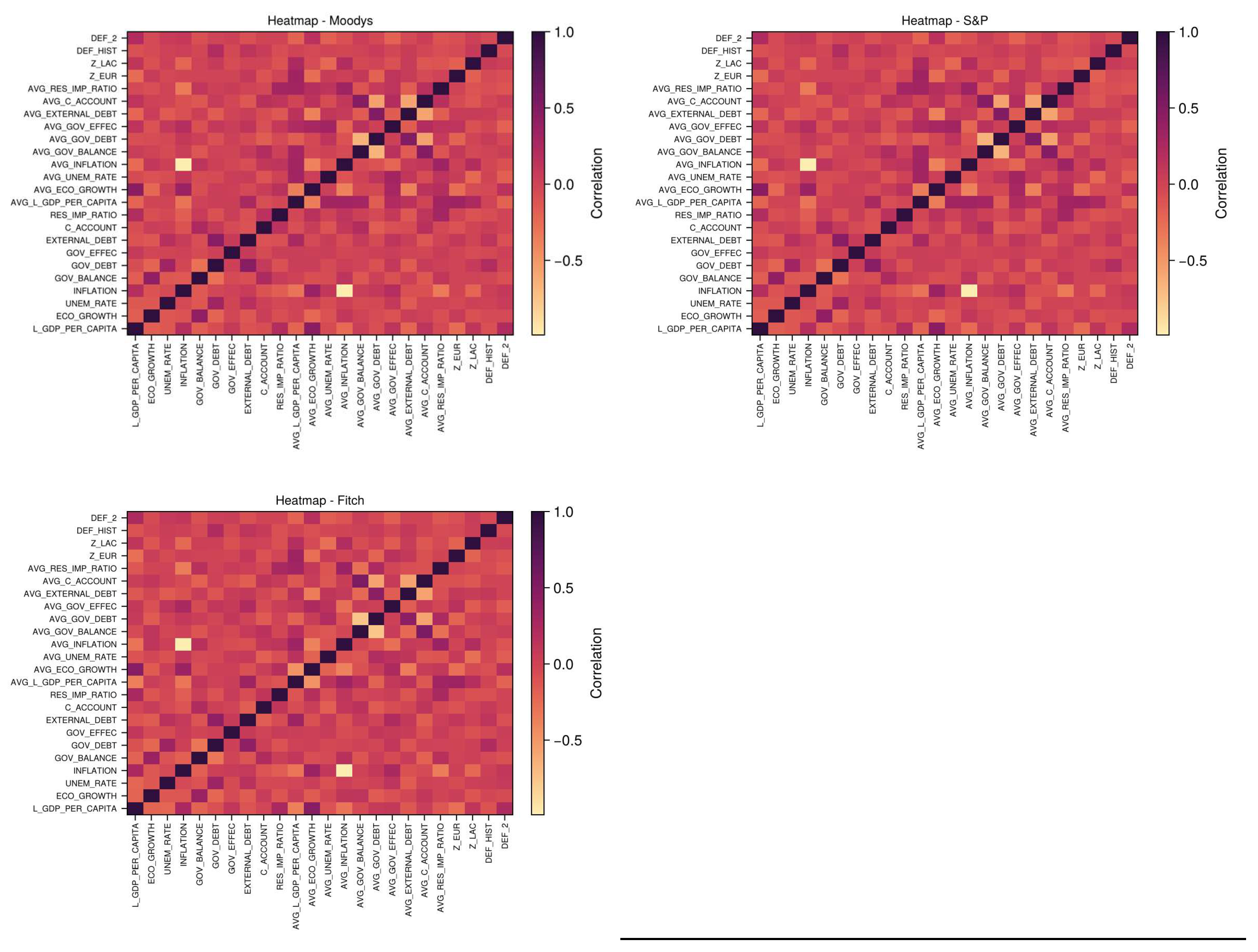
Table 4.1.
Posterior results for Moody’s.
| Variable | Mean | SD | ESS | MCMC Eff | ||||||||||||
|---|---|---|---|---|---|---|---|---|---|---|---|---|---|---|---|---|
| BGSS | LSS | NUTS | BGSS | LSS | NUTS | BGSS | LSS | NUTS | BGSS | LSS | NUTS | BGSS | LSS | NUTS | ||
| σ² | 2.885887 | 2.887541 | 2.897618 | 0.15996 | 0.14007 | 0.14293 | 31446 | 253 | 49756 | 4595 | 15 | 409 | 0.99998 | 1.00209 | 0.99998 | |
| L_GDP_PER_CAPITA | 0.7011*** | 0.723792*** | 0.72119*** | 0.13192 | 0.124 | 0.13031 | 33416 | 104 | 35326 | 4883 | 6 | 291 | 1.00004 | 1.0073 | 0.99999 | |
| ECO_GROWTH | 0.033199* | 0.031355** | 0.031393* | 0.01658 | 0.01638 | 0.01667 | 32944 | 421 | 42232 | 4814 | 25 | 348 | 1.00005 | 1.00835 | 0.99998 | |
| UNEM_RATE | -0.200221*** | -0.197571*** | -0.19719*** | 0.03438 | 0.03538 | 0.03474 | 32859 | 298 | 47120 | 4801 | 18 | 388 | 1.00004 | 1.00417 | 0.99998 | |
| INFLATION | -0.002432 | -0.002365 | -0.002515 | 0.00164 | 0.00168 | 0.00165 | 33404 | 462 | 65371 | 4881 | 28 | 538 | 1.00005 | 1.00552 | 0.99999 | |
| GOV_BALANCE | -0.081504*** | -0.080439*** | -0.077994*** | 0.02525 | 0.02411 | 0.02532 | 32773 | 274 | 38816 | 4789 | 17 | 319 | 1.00002 | 1.00023 | 1.0000 | |
| GOV_DEBT | -0.024248*** | -0.025408*** | -0.024975*** | 0.005 | 0.00517 | 0.00516 | 33321 | 548 | 48839 | 4869 | 33 | 402 | 1.00004 | 1.00107 | 1.00006 | |
| GOV_EFFEC | 0.297544** | 0.291483** | 0.3035*** | 0.12955 | 0.12605 | 0.13004 | 32440 | 152 | 58608 | 4740 | 9 | 482 | 1.00002 | 1.00051 | 0.99998 | |
| EXTERNAL_DEBT | 0.002401 | 0.00271 | 0.002794 | 0.00331 | 0.00331 | 0.00337 | 32507 | 673 | 51758 | 4750 | 41 | 426 | 1.0000 | 1.00102 | 1.0002 | |
| C_ACCOUNT | 0.017632 | 0.017454 | 0.015931 | 0.0137 | 0.01353 | 0.0138 | 34384 | 350 | 40364 | 5024 | 21 | 332 | 1.00007 | 1.0022 | 1.00007 | |
| RES_IMP_RATIO | 1.738925*** | 1.604894*** | 1.668966*** | 0.25933 | 0.20654 | 0.2567 | 33697 | 118 | 48261 | 4924 | 7 | 397 | 1.00007 | 1.00486 | 1.00003 | |
| AVG_L_GDP_PER_CAPITA | 0.966005*** | 0.969515*** | 0.961842*** | 0.04699 | 0.04705 | 0.04692 | 33299 | 100 | 23874 | 4865 | 6 | 196 | 1.00004 | 1.0214 | 1.00004 | |
| AVG_ECO_GROWTH | 0.171351*** | 0.181398*** | 0.190491*** | 0.04504 | 0.04706 | 0.04545 | 32479 | 115 | 35798 | 4746 | 7 | 295 | 1.00001 | 1.00262 | 1.00001 | |
| AVG_UNEM_RATE | -0.030615** | -0.030084** | -0.02877* | 0.01463 | 0.01414 | 0.01484 | 33878 | 216 | 37753 | 4950 | 13 | 311 | 1.00002 | 1.01947 | 0.99999 | |
| AVG_INFLATION | -0.006558*** | -0.006264*** | -0.006293*** | 0.00207 | 0.00214 | 0.00209 | 32958 | 281 | 58474 | 4816 | 17 | 481 | 1.0000 | 1.01041 | 1.00004 | |
| AVG_GOV_BALANCE | -0.187979*** | -0.186062*** | -0.17979*** | 0.03747 | 0.03643 | 0.03763 | 33121 | 145 | 31380 | 4840 | 9 | 258 | 1.00002 | 1.00771 | 0.99998 | |
| AVG_GOV_DEBT | -0.047317*** | -0.046672*** | -0.045741*** | 0.00449 | 0.00416 | 0.00448 | 33513 | 178 | 32907 | 4897 | 11 | 271 | 1.00001 | 1.00226 | 1.0000 | |
| AVG_GOV_EFFEC | 3.935795*** | 3.828428*** | 3.784918*** | 0.20067 | 0.1868 | 0.19995 | 33328 | 110 | 39544 | 4870 | 7 | 325 | 1.00003 | 1.01368 | 0.99998 | |
| AVG_EXTERNAL_DEBT | -0.002987 | -0.004075 | -0.004193 | 0.00441 | 0.0046 | 0.0045 | 33764 | 149 | 34915 | 4933 | 9 | 287 | 1.00005 | 1.00481 | 0.99998 | |
| AVG_C_ACCOUNT | 0.085831*** | 0.087451*** | 0.090616*** | 0.02695 | 0.02787 | 0.02739 | 33179 | 194 | 35757 | 4848 | 12 | 294 | 0.99999 | 1.0036 | 1.00001 | |
| AVG_RES_IMP_RATIO | 2.481859*** | 2.379836*** | 2.323865*** | 0.28807 | 0.24068 | 0.27502 | 32368 | 102 | 38985 | 4730 | 6 | 321 | 1.00022 | 1.00006 | 0.99999 | |
| Z_EUR | -1.101744*** | -1.037352*** | -0.944393*** | 0.30198 | 0.25892 | 0.29437 | 33373 | 99 | 35733 | 4876 | 6 | 294 | 1.00008 | 1.00211 | 1.00005 | |
| Z_LAC | -0.495625*** | -0.516329*** | -0.514551*** | 0.1498 | 0.14321 | 0.14972 | 33694 | 122 | 32441 | 4923 | 7 | 267 | 0.99998 | 1.00863 | 1 | |
| DEF_HIST | -1.65684*** | -1.412025*** | -1.425508*** | 0.43904 | 0.34262 | 0.41113 | 32668 | 97 | 58725 | 4773 | 6 | 483 | 0.99998 | 1.02084 | 1.00004 | |
| DEF_2 | -0.021771 | -0.026181 | -0.02761 | 0.01871 | 0.01918 | 0.01897 | 32573 | 313 | 38887 | 4760 | 19 | 320 | 1.00002 | 1.0002 | 1.00028 | |
| Coefficients marked with (*) represent significant variables at the 10% credibility level, (**) at 5%, and (***) at 1%. Mean denotes the marginal posterior mean, SD the Standard Deviation, ESS the Effective Sample Size, MCMC Eff the ESS per second and represents the potential scale reduction factor. Execution time (in seconds): BGSS = 6.843863, LSS = 16.511065, NUTS = 121.530931. | ||||||||||||||||
Table 4.2.
Posterior quantiles for Moody’s.
| Variable | Q 2.5 | Q 50 | Q 97.5 | |||||||||
|---|---|---|---|---|---|---|---|---|---|---|---|---|
| BGSS | LSS | NUTS | BGSS | LSS | NUTS | BGSS | LSS | NUTS | ||||
| σ² | 2.6077 | 2.6310 | 2.6307 | 2.8732 | 2.8826 | 2.8936 | 3.2321 | 3.1953 | 3.1908 | |||
| L_GDP_PER_CAPITA | 0.4345 | 0.5148 | 0.4677 | 0.7013 | 0.7098 | 0.7205 | 0.9714 | 0.9710 | 0.9768 | |||
| ECO_GROWTH | -0.0002 | 0.0007 | -0.0011 | 0.0332 | 0.0313 | 0.0314 | 0.0663 | 0.0631 | 0.0640 | |||
| UNEM_RATE | -0.2690 | -0.2672 | -0.2652 | -0.2001 | -0.1965 | -0.1971 | -0.1320 | -0.1283 | -0.1291 | |||
| INFLATION | -0.0057 | -0.0058 | -0.0057 | -0.0024 | -0.0023 | -0.0025 | 0.0009 | 0.0009 | 0.0007 | |||
| GOV_BALANCE | -0.1328 | -0.1264 | -0.1276 | -0.0815 | -0.0808 | -0.0780 | -0.0311 | -0.0318 | -0.0287 | |||
| GOV_DEBT | -0.0343 | -0.0352 | -0.0351 | -0.0242 | -0.0255 | -0.0250 | -0.0142 | -0.0150 | -0.0149 | |||
| GOV_EFFEC | 0.0434 | 0.0223 | 0.0458 | 0.2977 | 0.2903 | 0.3038 | 0.5511 | 0.5537 | 0.5593 | |||
| EXTERNAL_DEBT | -0.0043 | -0.0040 | -0.0038 | 0.0024 | 0.0027 | 0.0028 | 0.0090 | 0.0092 | 0.0094 | |||
| C_ACCOUNT | -0.0100 | -0.0091 | -0.0111 | 0.0177 | 0.0175 | 0.0159 | 0.0447 | 0.0451 | 0.0429 | |||
| RES_IMP_RATIO | 1.2267 | 1.1926 | 1.1667 | 1.7402 | 1.6086 | 1.6688 | 2.2543 | 1.9760 | 2.1708 | |||
| AVG_L_GDP_PER_CAPITA | 0.8704 | 0.8635 | 0.8701 | 0.9657 | 0.9697 | 0.9616 | 1.0622 | 1.0607 | 1.0544 | |||
| AVG_ECO_GROWTH | 0.0808 | 0.0890 | 0.1012 | 0.1715 | 0.1818 | 0.1905 | 0.2618 | 0.2755 | 0.2794 | |||
| AVG_UNEM_RATE | -0.0599 | -0.0591 | -0.0577 | -0.0307 | -0.0298 | -0.0288 | -0.0015 | -0.0037 | 0.0003 | |||
| AVG_INFLATION | -0.0107 | -0.0105 | -0.0104 | -0.0066 | -0.0063 | -0.0063 | -0.0025 | -0.0021 | -0.0022 | |||
| AVG_GOV_BALANCE | -0.2647 | -0.2550 | -0.2538 | -0.1882 | -0.1871 | -0.1798 | -0.1120 | -0.1126 | -0.1054 | |||
| AVG_GOV_DEBT | -0.0565 | -0.0550 | -0.0545 | -0.0473 | -0.0465 | -0.0458 | -0.0383 | -0.0383 | -0.0369 | |||
| AVG_GOV_EFFEC | 3.5320 | 3.4876 | 3.3900 | 3.9352 | 3.8281 | 3.7865 | 4.3363 | 4.2157 | 4.1719 | |||
| AVG_EXTERNAL_DEBT | -0.0119 | -0.0135 | -0.0130 | -0.0030 | -0.0039 | -0.0042 | 0.0059 | 0.0047 | 0.0046 | |||
| AVG_C_ACCOUNT | 0.0322 | 0.0344 | 0.0367 | 0.0859 | 0.0874 | 0.0907 | 0.1391 | 0.1429 | 0.1440 | |||
| AVG_RES_IMP_RATIO | 1.9175 | 1.8024 | 1.7858 | 2.4814 | 2.4111 | 2.3229 | 3.0512 | 2.7568 | 2.8620 | |||
| Z_EUR | -1.6982 | -1.5368 | -1.5200 | -1.0991 | -1.0149 | -0.9432 | -0.5117 | -0.5493 | -0.3701 | |||
| Z_LAC | -0.7871 | -0.7815 | -0.8093 | -0.4961 | -0.5260 | -0.5146 | -0.2023 | -0.2328 | -0.2202 | |||
| DEF_HIST | -2.5223 | -2.0836 | -2.2283 | -1.6572 | -1.3671 | -1.4258 | -0.7942 | -0.8163 | -0.6200 | |||
| DEF_2 | -0.0582 | -0.0652 | -0.0650 | -0.0217 | -0.0260 | -0.0276 | 0.0146 | 0.0092 | 0.0099 | |||
| Q. 2.5 denotes the 2.5th percentile, Q. 50 the posterior median, and Q. 97.5 the 97.5th percentile | ||||||||||||
Table 4.3.
Posterior results for S&P.
| Variable | Mean | SD | ESS | MCMC Eff | ||||||||||||
|---|---|---|---|---|---|---|---|---|---|---|---|---|---|---|---|---|
| BGSS | LSS | NUTS | BGSS | LSS | NUTS | BGSS | LSS | NUTS | BGSS | LSS | NUTS | BGSS | LSS | NUTS | ||
| σ² | 2.318965 | 2.335062 | 2.324916 | 0.12607 | 0.11992 | 0.11243 | 30304 | 205 | 44102 | 4310 | 12 | 308 | 0.99999 | 1.01067 | 1.00004 | |
| L_GDP_PER_CAPITA | 0.767119*** | 0.759171*** | 0.769463*** | 0.12134 | 0.12276 | 0.12002 | 32874 | 104 | 33555 | 4676 | 6 | 234 | 1.00007 | 1.02112 | 0.99998 | |
| ECO_GROWTH | 0.022749 | 0.021641 | 0.021972 | 0.0155 | 0.01574 | 0.01574 | 33396 | 406 | 39739 | 4750 | 24 | 277 | 1.00001 | 1.00027 | 1.00023 | |
| UNEM_RATE | -0.183592*** | -0.180318*** | -0.180961*** | 0.03156 | 0.03251 | 0.0324 | 33998 | 299 | 42863 | 4836 | 18 | 299 | 1.00003 | 1.00797 | 0.99998 | |
| INFLATION | -0.034064*** | -0.035413*** | -0.035169*** | 0.00599 | 0.00624 | 0.00607 | 33199 | 101 | 32220 | 4722 | 6 | 225 | 0.99999 | 1.0838 | 1.00007 | |
| GOV_BALANCE | -0.035609 | -0.034419 | -0.033345 | 0.02311 | 0.02301 | 0.02366 | 33962 | 274 | 36055 | 4831 | 16 | 252 | 0.99998 | 1.00092 | 1.00019 | |
| GOV_DEBT | -0.026141*** | -0.026775*** | -0.026599*** | 0.00443 | 0.00448 | 0.00446 | 33607 | 601 | 45555 | 4780 | 36 | 318 | 1.0000 | 0.99998 | 0.99998 | |
| GOV_EFFEC | 0.362216*** | 0.352998*** | 0.366654*** | 0.11606 | 0.12164 | 0.11704 | 32522 | 129 | 47396 | 4626 | 8 | 331 | 1.0000 | 1.0167 | 0.99998 | |
| EXTERNAL_DEBT | 0.004806* | 0.005265* | 0.005021* | 0.00288 | 0.00299 | 0.00291 | 32614 | 506 | 50363 | 4639 | 30 | 352 | 1.00025 | 1.00014 | 0.99999 | |
| C_ACCOUNT | -0.000852 | -0.001115 | -0.002015 | 0.01231 | 0.01278 | 0.01261 | 32499 | 373 | 38508 | 4623 | 22 | 269 | 0.99998 | 1.00536 | 1.00003 | |
| RES_IMP_RATIO | 1.569341*** | 1.505394*** | 1.511415*** | 0.24309 | 0.26027 | 0.24007 | 33109 | 106 | 41730 | 4710 | 6 | 291 | 1.00001 | 1.00839 | 1.0000 | |
| AVG_L_GDP_PER_CAPITA | 0.906611*** | 0.905527*** | 0.901847*** | 0.04227 | 0.04751 | 0.0418 | 32237 | 96 | 24346 | 4585 | 6 | 170 | 1.00000 | 1.00706 | 1.0000 | |
| AVG_ECO_GROWTH | 0.192813*** | 0.207674*** | 0.206126*** | 0.03998 | 0.03841 | 0.04053 | 33133 | 115 | 33240 | 4713 | 7 | 232 | 1.0000 | 1.0259 | 1.00002 | |
| AVG_UNEM_RATE | -0.026663** | -0.022853* | -0.023698* | 0.01303 | 0.01361 | 0.01329 | 33476 | 179 | 34886 | 4762 | 11 | 243 | 1.00001 | 1.00039 | 0.99998 | |
| AVG_INFLATION | -0.036191*** | -0.037283*** | -0.037079*** | 0.00616 | 0.00649 | 0.00624 | 33117 | 99 | 31619 | 4711 | 6 | 221 | 0.99999 | 1.0763 | 1.00008 | |
| AVG_GOV_BALANCE | -0.156306*** | -0.155096*** | -0.149759*** | 0.03409 | 0.03254 | 0.03442 | 33792 | 153 | 30159 | 4807 | 9 | 211 | 1.00000 | 1.01164 | 0.99998 | |
| AVG_GOV_DEBT | -0.041568*** | -0.040731*** | -0.04038*** | 0.004 | 0.00383 | 0.00403 | 33193 | 167 | 30931 | 4721 | 10 | 216 | 1.00009 | 1.01076 | 1.00012 | |
| AVG_GOV_EFFEC | 3.427806*** | 3.312355*** | 3.30559*** | 0.19458 | 0.21405 | 0.19347 | 31985 | 98 | 32594 | 4550 | 6 | 228 | 1.00002 | 1.01426 | 1.00003 | |
| AVG_EXTERNAL_DEBT | 0.005231 | 0.004434 | 0.004388 | 0.00397 | 0.00373 | 0.00398 | 30960 | 177 | 37997 | 4404 | 11 | 265 | 1.00002 | 1.00125 | 1.00002 | |
| AVG_C_ACCOUNT | 0.154754*** | 0.162322*** | 0.160486*** | 0.0241 | 0.02514 | 0.02443 | 32498 | 174 | 36270 | 4623 | 10 | 253 | 1.00003 | 1.00525 | 1.0001 | |
| AVG_RES_IMP_RATIO | 2.208102*** | 2.06659*** | 2.114971*** | 0.24505 | 0.20272 | 0.24371 | 33635 | 102 | 40257 | 4784 | 6 | 281 | 1.00004 | 1.01032 | 0.99999 | |
| Z_EUR | -0.583972** | -0.520761* | -0.470945* | 0.27606 | 0.31027 | 0.26773 | 32089 | 94 | 31857 | 4564 | 6 | 222 | 1.00005 | 1.01701 | 1.00002 | |
| Z_LAC | -0.746886*** | -0.736936*** | -0.739271*** | 0.12888 | 0.13395 | 0.12867 | 31928 | 105 | 37938 | 4542 | 6 | 265 | 1.00008 | 1.05171 | 0.99999 | |
| DEF_HIST | -1.52504*** | -1.464412*** | -1.340817*** | 0.39636 | 0.30799 | 0.3739 | 32065 | 101 | 43955 | 4561 | 6 | 307 | 1.0000 | 1.03444 | 0.99998 | |
| DEF_2 | -0.027989* | -0.030507 | -0.031213 | 0.01648 | 0.01706 | 0.01671 | 33968 | 316 | 43244 | 4832 | 19 | 302 | 0.99998 | 1.00835 | 0.99998 | |
| Coefficients marked with (*) represent significant variables at the 10% credibility level, (**) at 5%, and (***) at 1%. Mean denotes the marginal posterior mean, SD the Standard Deviation, ESS the Effective Sample Size, MCMC Eff the ESS per second and represents the potential scale reduction factor. Execution time (in seconds): BGSS = 7.030268, LSS = 16.824202, NUTS = 143.268156. | ||||||||||||||||
Table 4.4.
Posterior quantiles for S&P.
| Variable | Q 2.5 | Q 50 | Q 97.5 | |||||||||
|---|---|---|---|---|---|---|---|---|---|---|---|---|
| BGSS | LSS | NUTS | BGSS | LSS | NUTS | BGSS | LSS | NUTS | ||||
| σ² | 2.0987 | 2.1145 | 2.1131 | 2.3088 | 2.3325 | 2.3216 | 2.5950 | 2.5793 | 2.5533 | |||
| L_GDP_PER_CAPITA | 0.5212 | 0.5024 | 0.5329 | 0.7671 | 0.7604 | 0.7705 | 1.0147 | 1.0012 | 1.0047 | |||
| ECO_GROWTH | -0.0086 | -0.0095 | -0.0092 | 0.0228 | 0.0211 | 0.0220 | 0.0536 | 0.0528 | 0.0528 | |||
| UNEM_RATE | -0.2469 | -0.2423 | -0.2449 | -0.1834 | -0.1803 | -0.1811 | -0.1207 | -0.1151 | -0.1176 | |||
| INFLATION | -0.0459 | -0.0473 | -0.0470 | -0.0341 | -0.0351 | -0.0352 | -0.0221 | -0.0238 | -0.0232 | |||
| GOV_BALANCE | -0.0818 | -0.0776 | -0.0795 | -0.0356 | -0.0342 | -0.0334 | 0.0110 | 0.0096 | 0.0130 | |||
| GOV_DEBT | -0.0350 | -0.0357 | -0.0353 | -0.0261 | -0.0266 | -0.0266 | -0.0173 | -0.0182 | -0.0179 | |||
| GOV_EFFEC | 0.1347 | 0.1108 | 0.1375 | 0.3622 | 0.3504 | 0.3666 | 0.5911 | 0.5839 | 0.5938 | |||
| EXTERNAL_DEBT | -0.0009 | -0.0005 | -0.0008 | 0.0048 | 0.0053 | 0.0050 | 0.0106 | 0.0111 | 0.0107 | |||
| C_ACCOUNT | -0.0253 | -0.0256 | -0.0268 | -0.0009 | -0.0016 | -0.0020 | 0.0238 | 0.0253 | 0.0228 | |||
| RES_IMP_RATIO | 1.0891 | 1.0780 | 1.0397 | 1.5693 | 1.4716 | 1.5124 | 2.0506 | 2.1155 | 1.9801 | |||
| AVG_L_GDP_PER_CAPITA | 0.8199 | 0.8160 | 0.8210 | 0.9064 | 0.8976 | 0.9016 | 0.9924 | 1.0047 | 0.9841 | |||
| AVG_ECO_GROWTH | 0.1124 | 0.1280 | 0.1264 | 0.1927 | 0.2061 | 0.2061 | 0.2735 | 0.2897 | 0.2855 | |||
| AVG_UNEM_RATE | -0.0524 | -0.0501 | -0.0496 | -0.0266 | -0.0229 | -0.0237 | -0.0009 | 0.0037 | 0.0022 | |||
| AVG_INFLATION | -0.0484 | -0.0499 | -0.0493 | -0.0362 | -0.0369 | -0.0371 | -0.0239 | -0.0253 | -0.0248 | |||
| AVG_GOV_BALANCE | -0.2248 | -0.2197 | -0.2176 | -0.1564 | -0.1559 | -0.1495 | -0.0865 | -0.0914 | -0.0824 | |||
| AVG_GOV_DEBT | -0.0497 | -0.0484 | -0.0483 | -0.0416 | -0.0408 | -0.0404 | -0.0334 | -0.0331 | -0.0325 | |||
| AVG_GOV_EFFEC | 3.0375 | 2.8906 | 2.9302 | 3.4278 | 3.3154 | 3.3038 | 3.8183 | 3.7223 | 3.6858 | |||
| AVG_EXTERNAL_DEBT | -0.0028 | -0.0027 | -0.0035 | 0.0052 | 0.0044 | 0.0044 | 0.0131 | 0.0121 | 0.0122 | |||
| AVG_C_ACCOUNT | 0.1069 | 0.1172 | 0.1125 | 0.1547 | 0.1612 | 0.1606 | 0.2018 | 0.2160 | 0.2083 | |||
| AVG_RES_IMP_RATIO | 1.7249 | 1.6670 | 1.6372 | 2.2093 | 2.0747 | 2.1161 | 2.6869 | 2.4232 | 2.5883 | |||
| Z_EUR | -1.1329 | -1.1587 | -0.9926 | -0.5840 | -0.5140 | -0.4694 | -0.0339 | 0.1302 | 0.0484 | |||
| Z_LAC | -1.0012 | -1.0234 | -0.9925 | -0.7463 | -0.7337 | -0.7390 | -0.4952 | -0.4764 | -0.4864 | |||
| DEF_HIST | -2.3147 | -2.1400 | -2.0708 | -1.5250 | -1.4554 | -1.3397 | -0.7512 | -0.8914 | -0.6081 | |||
| DEF_2 | -0.0604 | -0.0646 | -0.0638 | -0.0280 | -0.0308 | -0.0312 | 0.0044 | 0.0036 | 0.0014 | |||
| Q. 2.5 denotes the 2.5th percentile, Q. 50 the posterior median, and Q. 97.5 the 97.5th percentile | ||||||||||||
Table 4.5.
Posterior results for Fitch.
| Variable | Mean | SD | ESS | MCMC Eff | ||||||||||||
|---|---|---|---|---|---|---|---|---|---|---|---|---|---|---|---|---|
| BGSS | LSS | NUTS | BGSS | LSS | NUTS | BGSS | LSS | NUTS | BGSS | LSS | NUTS | BGSS | LSS | NUTS | ||
| σ² | 2.128879 | 2.153565 | 2.137422 | 0.13451 | 0.12646 | 0.11804 | 29968 | 202 | 48726 | 5084 | 14 | 387 | 0.99999 | 1.00856 | 1.00001 | |
| L_GDP_PER_CAPITA | 0.618337*** | 0.621537*** | 0.61013*** | 0.12867 | 0.13806 | 0.12937 | 32907 | 101 | 35174 | 5583 | 7 | 280 | 1.00004 | 1.01005 | 0.99998 | |
| ECO_GROWTH | 0.003813 | 0.003283 | 0.002379 | 0.01501 | 0.01512 | 0.01516 | 33339 | 355 | 44555 | 5656 | 24 | 354 | 1.00004 | 1.00113 | 0.99999 | |
| UNEM_RATE | -0.223019*** | -0.221894*** | -0.224222*** | 0.03452 | 0.03379 | 0.03504 | 33061 | 262 | 40404 | 5609 | 18 | 321 | 1.0000 | 1.00216 | 1.00002 | |
| INFLATION | -0.036528*** | -0.036552*** | -0.037804*** | 0.00638 | 0.00716 | 0.00645 | 33114 | 100 | 30386 | 5618 | 7 | 242 | 0.99998 | 1.02986 | 0.99998 | |
| GOV_BALANCE | -0.017185 | -0.01457 | -0.014705 | 0.02265 | 0.02365 | 0.02299 | 33101 | 278 | 39318 | 5616 | 19 | 313 | 1.00021 | 0.99998 | 0.99999 | |
| GOV_DEBT | -0.030152*** | -0.030601*** | -0.030441*** | 0.00476 | 0.00482 | 0.00482 | 33897 | 489 | 48334 | 5751 | 33 | 384 | 1.0000 | 1.00408 | 1.00002 | |
| GOV_EFFEC | 0.66914*** | 0.6599*** | 0.677775*** | 0.16206 | 0.15361 | 0.16187 | 32941 | 117 | 51927 | 5589 | 8 | 413 | 1.00011 | 1.0094 | 0.99998 | |
| EXTERNAL_DEBT | 0.006461** | 0.007494** | 0.007244** | 0.00322 | 0.00332 | 0.00327 | 33291 | 400 | 52155 | 5648 | 27 | 415 | 0.99998 | 1.00115 | 1.00008 | |
| C_ACCOUNT | -0.01159 | -0.012883 | -0.011847 | 0.01191 | 0.01228 | 0.01212 | 33958 | 389 | 42667 | 5761 | 26 | 339 | 1.00007 | 1.00053 | 0.99999 | |
| RES_IMP_RATIO | 1.28*** | 1.293691*** | 1.233702*** | 0.27517 | 0.30748 | 0.26863 | 32679 | 96 | 42197 | 5544 | 6 | 335 | 1.00003 | 1.00148 | 0.99998 | |
| AVG_L_GDP_PER_CAPITA | 0.832724*** | 0.840326*** | 0.84034*** | 0.04643 | 0.0482 | 0.04656 | 32710 | 95 | 25061 | 5549 | 6 | 199 | 0.99998 | 1.02034 | 1.00009 | |
| AVG_ECO_GROWTH | 0.298305*** | 0.312665*** | 0.312817*** | 0.04222 | 0.04284 | 0.04305 | 33499 | 121 | 34523 | 5683 | 8 | 274 | 1.00005 | 1.00889 | 0.99999 | |
| AVG_UNEM_RATE | 0.046203*** | 0.043533*** | 0.044155*** | 0.0158 | 0.01681 | 0.01612 | 33329 | 179 | 35027 | 5654 | 12 | 278 | 1.00015 | 1.00773 | 0.99998 | |
| AVG_INFLATION | -0.040103*** | -0.039791*** | -0.041053*** | 0.0065 | 0.00734 | 0.00658 | 33263 | 99 | 30002 | 5643 | 7 | 239 | 0.99998 | 1.02791 | 1.00002 | |
| AVG_GOV_BALANCE | -0.157251*** | -0.160289*** | -0.153654*** | 0.03561 | 0.03422 | 0.0358 | 31859 | 140 | 33647 | 5405 | 9 | 268 | 0.99999 | 1.0156 | 1.00000 | |
| AVG_GOV_DEBT | -0.054262*** | -0.053019*** | -0.052409*** | 0.00467 | 0.00456 | 0.00469 | 32840 | 151 | 34307 | 5571 | 10 | 273 | 1.00001 | 1.00294 | 1.00015 | |
| AVG_GOV_EFFEC | 3.647252*** | 3.475004*** | 3.484661*** | 0.21203 | 0.2285 | 0.21012 | 32984 | 101 | 40531 | 5596 | 7 | 322 | 1.00018 | 1.00443 | 0.99998 | |
| AVG_EXTERNAL_DEBT | 0.008893** | 0.007417* | 0.007292* | 0.00406 | 0.00415 | 0.00408 | 33117 | 166 | 35047 | 5619 | 11 | 279 | 1.00001 | 1.00001 | 0.99998 | |
| AVG_C_ACCOUNT | 0.198169*** | 0.200779*** | 0.200818*** | 0.02512 | 0.02409 | 0.02548 | 33584 | 184 | 38224 | 5698 | 12 | 304 | 1.00004 | 1.00783 | 1.0000 | |
| AVG_RES_IMP_RATIO | 3.215205*** | 2.946733*** | 2.996444*** | 0.28814 | 0.30067 | 0.27781 | 32772 | 94 | 36065 | 5560 | 6 | 287 | 1.00008 | 1.02068 | 0.99998 | |
| Z_EUR | -0.618842** | -0.506493** | -0.513542** | 0.26605 | 0.24357 | 0.26128 | 32899 | 100 | 36735 | 5581 | 7 | 292 | 0.99998 | 1.01373 | 1.00003 | |
| Z_LAC | -0.369574*** | -0.387158*** | -0.392842*** | 0.14418 | 0.14877 | 0.14416 | 33030 | 110 | 39145 | 5604 | 7 | 311 | 1.00012 | 1.0151 | 0.99999 | |
| DEF_HIST | -0.363983 | -0.323328 | -0.319194 | 0.48912 | 0.4949 | 0.44282 | 34207 | 91 | 48619 | 5803 | 6 | 387 | 0.99999 | 1.11179 | 1.00005 | |
| DEF_2 | 0.002077 | -0.002407 | -0.001834 | 0.01679 | 0.01717 | 0.01707 | 31935 | 327 | 47552 | 5418 | 22 | 378 | 1.00005 | 1.00116 | 0.99998 | |
| Coefficients marked with (*) represent significant variables at the 10% credibility level, (**) at 5%, and (***) at 1%. Mean denotes the marginal posterior mean, SD the Standard Deviation, ESS the Effective Sample Size, MCMC Eff the ESS per second and represents the potential scale reduction factor. Execution time (in seconds): BGSS = 7.030268, LSS = 16.824202, NUTS = 143.268156. | ||||||||||||||||
Table 4.6.
Posterior quantiles for Fitch.
| Variable | Q 2.5 | Q 50 | Q 97.5 | |||||||||
|---|---|---|---|---|---|---|---|---|---|---|---|---|
| BGSS | LSS | NUTS | BGSS | LSS | NUTS | BGSS | LSS | NUTS | ||||
| σ² | 1.9003 | 1.9105 | 1.9177 | 2.1171 | 2.1480 | 2.1334 | 2.4220 | 2.4065 | 2.3806 | |||
| L_GDP_PER_CAPITA | 0.3573 | 0.3324 | 0.3556 | 0.6180 | 0.6237 | 0.6102 | 0.8777 | 0.8564 | 0.8652 | |||
| ECO_GROWTH | -0.0262 | -0.0254 | -0.0274 | 0.0038 | 0.0033 | 0.0024 | 0.0339 | 0.0328 | 0.0320 | |||
| UNEM_RATE | -0.2920 | -0.2842 | -0.2926 | -0.2231 | -0.2228 | -0.2243 | -0.1537 | -0.1536 | -0.1555 | |||
| INFLATION | -0.0492 | -0.0500 | -0.0504 | -0.0365 | -0.0363 | -0.0378 | -0.0239 | -0.0224 | -0.0253 | |||
| GOV_BALANCE | -0.0625 | -0.0618 | -0.0600 | -0.0172 | -0.0138 | -0.0148 | 0.0285 | 0.0308 | 0.0305 | |||
| GOV_DEBT | -0.0397 | -0.0399 | -0.0399 | -0.0302 | -0.0306 | -0.0304 | -0.0205 | -0.0209 | -0.0210 | |||
| GOV_EFFEC | 0.3499 | 0.3868 | 0.3574 | 0.6690 | 0.6507 | 0.6781 | 0.9879 | 0.9838 | 0.9928 | |||
| EXTERNAL_DEBT | 0.0000 | 0.0011 | 0.0008 | 0.0064 | 0.0075 | 0.0073 | 0.0130 | 0.0143 | 0.0136 | |||
| C_ACCOUNT | -0.0352 | -0.0364 | -0.0357 | -0.0117 | -0.0129 | -0.0119 | 0.0121 | 0.0118 | 0.0119 | |||
| RES_IMP_RATIO | 0.7326 | 0.7489 | 0.7057 | 1.2807 | 1.3126 | 1.2326 | 1.8272 | 1.7941 | 1.7599 | |||
| AVG_L_GDP_PER_CAPITA | 0.7380 | 0.7465 | 0.7498 | 0.8327 | 0.8411 | 0.8402 | 0.9274 | 0.9330 | 0.9320 | |||
| AVG_ECO_GROWTH | 0.2136 | 0.2195 | 0.2285 | 0.2982 | 0.3137 | 0.3127 | 0.3825 | 0.3938 | 0.3977 | |||
| AVG_UNEM_RATE | 0.0141 | 0.0116 | 0.0125 | 0.0461 | 0.0429 | 0.0442 | 0.0778 | 0.0756 | 0.0757 | |||
| AVG_INFLATION | -0.0531 | -0.0536 | -0.0539 | -0.0401 | -0.0397 | -0.0410 | -0.0272 | -0.0252 | -0.0281 | |||
| AVG_GOV_BALANCE | -0.2299 | -0.2233 | -0.2241 | -0.1572 | -0.1613 | -0.1535 | -0.0842 | -0.0913 | -0.0835 | |||
| AVG_GOV_DEBT | -0.0638 | -0.0622 | -0.0616 | -0.0543 | -0.0529 | -0.0524 | -0.0449 | -0.0444 | -0.0432 | |||
| AVG_GOV_EFFEC | 3.2251 | 3.0017 | 3.0717 | 3.6481 | 3.4859 | 3.4846 | 4.0691 | 3.9513 | 3.8974 | |||
| AVG_EXTERNAL_DEBT | 0.0008 | -0.0007 | -0.0007 | 0.0089 | 0.0075 | 0.0073 | 0.0171 | 0.0153 | 0.0153 | |||
| AVG_C_ACCOUNT | 0.1486 | 0.1519 | 0.1508 | 0.1981 | 0.2009 | 0.2007 | 0.2476 | 0.2460 | 0.2512 | |||
| AVG_RES_IMP_RATIO | 2.6514 | 2.2865 | 2.4484 | 3.2145 | 2.9594 | 2.9976 | 3.7879 | 3.5426 | 3.5427 | |||
| Z_EUR | -1.1465 | -0.9526 | -1.0284 | -0.6196 | -0.5140 | -0.5140 | -0.0951 | -0.0288 | -0.0022 | |||
| Z_LAC | -0.6538 | -0.7040 | -0.6747 | -0.3696 | -0.3800 | -0.3923 | -0.0848 | -0.1271 | -0.1085 | |||
| DEF_HIST | -1.3285 | -1.2030 | -1.1865 | -0.3614 | -0.3556 | -0.3195 | 0.5862 | 0.7719 | 0.5520 | |||
| DEF_2 | -0.0308 | -0.0349 | -0.0352 | 0.0021 | -0.0024 | -0.0019 | 0.0351 | 0.0311 | 0.0317 | |||
| Q. 2.5 denotes the 2.5th percentile, Q. 50 the posterior median, and Q. 97.5 the 97.5th percentile | ||||||||||||
The estimation results for Moody’s, S&P, and Fitch consistently reaffirm the pivotal role of macroeconomic and fiscal fundamentals, as previously highlighted in the literature. Across all three agencies, both short-run factors, such as GDP growth (ECO_GROWTH) and current unemployment rates (UNEM_RATE), and long-run indicators, such as averaged GDP per capita (AVG_L_GDP_PER_CAPITA), long-term inflation performance (AVG_INFLATION), and historical fiscal balances (AVG_GOV_BALANCE), are highly influential. Specifically, higher levels of GDP per capita (L_GDP_PER_CAPITA) and robust economic growth (ECO_GROWTH) consistently correlate with better credit ratings. In the short run, even marginal improvements in the economic environment can translate into more favourable ratings. Over the long term, the averaged income level (AVG_L_GDP_PER_CAPITA) and sustained growth trends (AVG_ECO_GROWTH) contribute to a stable and positive rating trajectory.
Variables such as government debt levels (GOV_DEBT) and budget balances (GOV_BALANCE) exert a powerful influence. Larger government debt ratios (GOV_DEBT) and persistent deficits (AVG_GOV_BALANCE) are associated with lower ratings, underscoring market concerns about fiscal sustainability. In the long term, the average stance of fiscal indicators (AVG_GOV_BALANCE, AVG_GOV_DEBT) matters even more, with persistent fiscal imbalances leading to systematically worse ratings. Higher unemployment rates (UNEM_RATE) have a negative impact on credit ratings, indicating concerns about a country’s ability to generate sustainable income and maintain social stability.
Inflation (INFLATION) likewise plays a key role. While short-term inflation episodes may signal transitory imbalances, the long-run inflation average (AVG_INFLATION) is crucial for capturing a country’s track record of price stability, and thus its perceived macroeconomic credibility. Governance effectiveness (GOV_EFFEC) emerges as a robust determinant. Better institutional frameworks and credible, transparent policymaking deliver higher ratings. Over the long run, institutions that consistently support sound policy execution and prevent destabilizing shocks help build confidence among rating agencies.
External debt levels (EXTERNAL_DEBT), current account balances (C_ACCOUNT), and reserve-to-import ratios (RES_IMP_RATIO) reflect external vulnerability. Higher reserve adequacy and stronger external positions (AVG_EXTERNAL_DEBT, AVG_C_ACCOUNT, AVG_RES_IMP_RATIO) are associated with more favourable ratings. Moreover, regional dummy variables (such as those for European (Z_EUR) or Latin American (Z_LAC) countries) and default history indicators (DEF_HIST, DEF_2) highlight geographical and historical contexts influencing credit perceptions.
In terms of differences among agencies, while Moody’s, S&P, and Fitch generally respond similarly to the main macroeconomic and institutional drivers, some nuances emerge. For instance, certain parameters may be estimated with more precision or show slightly varying magnitudes across agencies, reflecting differences in agencies’ rating methodologies or the scope of their information sets. Nonetheless, the broad pattern of significance and the direction of effects remain consistent across all three, confirming the robustness of the identified determinants.
Regarding the performance of our algorithm, BGSS offers clear advantages. While all three methods converge to similar posterior estimates, the BGSS sampler excels in terms of computational efficiency and effective sample sizes (ESS). These features are reflected in higher ESS per second and robust convergence diagnostics, which indicate that BGSS can produce more stable and reliable inference within shorter run times. By contrast, LSS required significant tuning (λ=10,000) and extended chains to reach acceptable convergence, and NUTS, although a sophisticated gradient-based method, demanded substantially more computational time for a similar effective sample size.
The BGSS method’s ability to manage model complexity, incorporate parameter uncertainty through a straightforward Bayesian linear framework, and handle potential multicollinearity (in part aided by QR decompositions) underscores its flexibility. In addition, the stable and efficient performance of BGSS across different agencies’ datasets, each with slightly different sample sizes and missing data patterns, highlights the robustness and scalability of the approach.
In summary, the results reinforce the established understanding that both short-run economic signals and long-run structural characteristics are integral to sovereign credit rating formation. Macroeconomic stability, prudent fiscal management, competent governance, and favourable external positions all contribute decisively to higher sovereign ratings. The Bayesian panel approach, spearheaded by the BGSS sampler, not only validates these relationships with precision but also streamlines the estimation process, offering a powerful tool for policymakers, investors, and researchers seeking a more efficient and comprehensive assessment of sovereign creditworthiness.
4. Conclusion
In conclusion, this paper introduces the Bayesian Gibbs Slice Sampler (BGSS), a novel MCMC approach that successfully integrates the advantages of slice sampling with Bayesian inference, without requiring intricate tuning or gradient-based computations. The simulation study and empirical application consistently demonstrate that BGSS delivers superior efficiency, measured by higher effective sample sizes per second, compared to established methods such as Latent Slice Sampling (LSS) and the No-U-Turn Sampler (NUTS). By relying on a Bayesian framework, QR decompositions, and a component-wise conditional updating strategy, BGSS effectively mitigates random walk behaviour and ensures rapid and stable posterior exploration.
From an econometric perspective, the application to sovereign credit ratings reaffirms the critical role of both short- and long-term macroeconomic determinants. Factors such as GDP per capita, inflation, fiscal balances, and institutional quality exert persistent and meaningful influence on credit assessments assigned by major rating agencies. The enhanced inference offered by BGSS, translating into higher-quality posterior estimates and reduced computational overhead per effective sample, stands to benefit policymakers, investors, and researchers. This approach not only streamlines the estimation process but also provides more robust guidance for interpreting the impact of macroeconomic fundamentals on sovereign risk.
Future research could expand the current framework in several directions. First, exploring the performance of BGSS under alternative model specifications, such as nonlinear or time-varying parameter models, could further highlight its versatility. Additionally, integrating non-Gaussian distributions or hierarchical structures may offer insights into more complex data-generating processes, broadening the applicability of BGSS to a wide range of empirical problems. Finally, investigating the potential integration of BGSS with different data transformations could further reduce execution times, making it an even more practical tool for large-scale Bayesian inference tasks. Overall, the contributions of this paper suggest that BGSS has the potential to become a valuable component of the econometrician’s toolkit. Its robustness, efficiency, and ease of implementation invite further inquiry into its performance in increasingly complex and data-intensive environments, thereby opening new avenues for methodological refinement and empirical exploration.
References
- Afonso, A., Gomes, P., & Rother, P. (2007). What’hides’ behind sovereign debt ratings? ECB Working Paper.
- Afonso, A., Gomes, P., & Rother, P. (2011). Short-and long-run determinants of sovereign debt credit ratings. International Journal of Finance & Economics, 16(1), 1–15. [CrossRef]
- Bezanson, J., Edelman, A., Karpinski, S., & Shah, V. B. (2017). Julia: A fresh approach to numerical computing. SIAM Review, 59(1), 65–98. [CrossRef]
- Cantor, R., & Packer, F. (1996). Determinants and impact of sovereign credit ratings. Economic Policy Review, 2(2). [CrossRef]
- Carpenter, B., Gelman, A., Hoffman, M. D., Lee, D., Goodrich, B., Betancourt, M., Brubaker, M. A., Guo, J., Li, P., & Riddell, A. (2017). Stan: A probabilistic programming language. Journal of Statistical Software, 76. https://doi.org/10.18637/jss.v076.i01. [CrossRef]
- Damlen, P., Wakefield, J., & Walker, S. (1999). Gibbs sampling for Bayesian non-conjugate and hierarchical models by using auxiliary variables. Journal of the Royal Statistical Society: Series B (Statistical Methodology), 61(2), 331–344. [CrossRef]
- Ge, H., Xu, K., & Ghahramani, Z. (2018). Turing: A Language for Flexible Probabilistic Inference. Proceedings of the Twenty-First International Conference on Artificial Intelligence and Statistics, 1682–1690. https://proceedings.mlr.press/v84/ge18b.html.
- Gelman, A., Carlin, J. B., Stern, H. S., & Rubin, D. B. (2014). Bayesian data analysis. Chapman and Hall/CRC.
- Geweke, J. (2005). Contemporary Bayesian econometrics and statistics. John Wiley & Sons.
- Girolami, M., & Calderhead, B. (2011). Riemann manifold langevin and hamiltonian monte carlo methods. Journal of the Royal Statistical Society Series B: Statistical Methodology, 73(2), 123–214.
- Goodman, J., & Weare, J. (2010). Ensemble samplers with affine invariance. Communications in Applied Mathematics and Computational Science, 5(1), 65–80.
- Hastings, W. K. (1970). Monte Carlo sampling methods using Markov chains and their applications.
- Herce, Á., & Salvador, M. (2024). Instrument Selection in Panel Data Models with Endogeneity: A Bayesian Approach. Econometrics, 12(4), 36. [CrossRef]
- Hoffman, M. D., & Gelman, A. (2014). The No-U-Turn sampler: Adaptively setting path lengths in Hamiltonian Monte Carlo. J. Mach. Learn. Res., 15(1), 1593–1623.
- Jeffreys, H. (1961). The theory of probability (3rd ed.). Clarendon Press, Oxford.
- Karamanis, M., & Beutler, F. (2021). Ensemble slice sampling: Parallel, black-box and gradient-free inference for correlated & multimodal distributions. Statistics and Computing, 31, 1–18.
- Kim, S.-J., & Wu, E. (2008). Sovereign credit ratings, capital flows and financial sector development in emerging markets. Emerging Markets Review, 9(1), 17–39. https://doi.org/10.1016/j.ememar.2007.06.001. [CrossRef]
- Koepke, R. (2019). What Drives Capital Flows to Emerging Markets? A Survey of the Empirical Literature. Journal of Economic Surveys, 33(2), 516–540. https://doi.org/10.1111/joes.12273. [CrossRef]
- Li, Y., & Walker, S. G. (2023). A latent slice sampling algorithm. Computational Statistics & Data Analysis, 179, 107652. https://doi.org/10.1016/j.csda.2022.107652. [CrossRef]
- Mellios, C., & Paget-Blanc, E. (2006). Which factors determine sovereign credit ratings? The European Journal of Finance, 12(4), 361–377.
- Mira, A., & Tierney, L. (2002). Efficiency and convergence properties of slice samplers. Scandinavian Journal of Statistics, 29(1), 1–12. [CrossRef]
- Murray, I., Adams, R., & MacKay, D. (2010). Elliptical slice sampling. Proceedings of the Thirteenth International Conference on Artificial Intelligence and Statistics, 541–548.
- Murray, I., & Adams, R. P. (2010). Slice sampling covariance hyperparameters of latent Gaussian models. Advances in Neural Information Processing Systems, 23.
- Neal, R. M. (2003). Slice sampling. The Annals of Statistics, 31(3), 705–767.
- Neal, R. M. (2011). MCMC using Hamiltonian dynamics. Handbook of Markov Chain Monte Carlo, 2(11), 2.
- Reusens, P., & Croux, C. (2017). Sovereign credit rating determinants: A comparison before and after the European debt crisis. Journal of Banking & Finance, 77, 108–121. [CrossRef]
- Roberts, G. O., & Rosenthal, J. S. (1999). Convergence of slice sampler Markov chains. Journal of the Royal Statistical Society Series B: Statistical Methodology, 61(3), 643–660.
- Schär, P., Habeck, M., & Rudolf, D. (2023). Gibbsian polar slice sampling. International Conference on Machine Learning, 30204–30223.
- Tibbits, M. M., Groendyke, C., Haran, M., & Liechty, J. C. (2014). Automated factor slice sampling. Journal of Computational and Graphical Statistics, 23(2), 543–563.
- Wooldridge, J. M. (2005). Fixed-effects and related estimators for correlated random-coefficient and treatment-effect panel data models. Review of Economics and Statistics, 87(2), 385–390. [CrossRef]
Disclaimer/Publisher’s Note: The statements, opinions and data contained in all publications are solely those of the individual author(s) and contributor(s) and not of MDPI and/or the editor(s). MDPI and/or the editor(s) disclaim responsibility for any injury to people or property resulting from any ideas, methods, instructions or products referred to in the content. |
© 2025 by the authors. Licensee MDPI, Basel, Switzerland. This article is an open access article distributed under the terms and conditions of the Creative Commons Attribution (CC BY) license (http://creativecommons.org/licenses/by/4.0/).
Copyright: This open access article is published under a Creative Commons CC BY 4.0 license, which permit the free download, distribution, and reuse, provided that the author and preprint are cited in any reuse.


