A Different Way to Count, Add, and Multiply

1. Introduction

The Roman numeric system carried human computations throughout the Roman empire and well into the Middle Ages. It was limited in its expression abilities by the list of symbols used for large numbers. A dramatic revolution in computation, and hence in commerce, and civilization happened when power expressions came forth wherein any number x could be written as:

x = ∑a_nbⁿ for n=0,1,2,.. where 0 ≤ a_n ≤ b-1

This exponential method advanced counting by allowing for a limited number of symbols (b) to systematically express any number, however large.

While for human counting the most popular value for the base b is b=10, many lament that b=12 was not chosen by our ancestors, having more divisors than 10. Today b=2. 8. 16 are common and useful bases.

Innovation Science [8] calls for a revisiting established premises, searching for a useful modification. The essential advantage of the so called, “positional system” of counting is the grouping of numbers to very larger groups 10, 100, 1000, .... then counting these groups.

Grouping can be done on a fixed basis through power raising, but not necessarily so. In the existing system the power base, b, is an arbitrary choice. Is there a natural choice?

Yes, there is: incremental counting. Instead of 0,1,2,4,8,16. where counting starts from zero:

(0), (0,1), (0,1,2,3), (0,1,2,3,4,5,6,7), (0,1,2,3,4,5,6,7,8,9,10,11,12,13,14,15).....

We can count successively:

(0), (1), (2,3), (4,5,6), (7,8,9,10), (11,12,13,14,15), .....

counting these groups with our numeral symbols:

[0] = (0), [1] = (1), [2] = (2,3), [3] = (4,5,6), [4] = (7,8,9,10), [5] = (11,12,13,14,15)

Accordingly number 5 is expressed as number count 2 in group 3, and 14 is number count 4 in group 5, etc.

The grouping here increases incrementally not exponentially, but they add-up rather than start from 0. And most importantly this grouping, (let’s call it numeration) does not rely on an arbitrarily selected base b -- it is natural grouping.

It is of great interest to explore more ways to write down the list of natural numbers. Given the power of AI to find hidden pattern, this numerization representation is worth the study.

2. Methodology

Natural number, n is defined as something that is not 1, not 2, not 3,....not (n-1): n ≠ i. for i=1,2,...(n-1).

These natural numbers are merely a succession of distinctions without any further attribution. In other words, natural numbers are highly abstracted, they only express mutual distinction and order of creation. But they can be further abstracted as entities that qualify as numbers but which are not specified as to being one number or another in particular.

So abstracted a natural number is designated by the Hebrew letter “Shin”, ש, the first letter of the word ’sky’ in Hebrew (“Shamaeem”, שמיים ), which is the first created entity in the Biblical account. Shin represents a number with unspecified designation.

Written as 1,2,3,... the natural numbers are mutually distinct, and no two of them are equivalent. However, listed as. ש, ש, ש... the list comprises elements of equivalence -- all being natural numbers. Equivalence and distinction are in the eyes of the beholder (the mathematician).

Given the unspecified list: ש, ש, ש... the mathematician wishes to express it as a series of natural numbers: 1, 2, 3, ... To that aim the mathematician defines one element as the first ש, and calls it “1”. In order to define a “2” in the ש, ש, ... list the mathematician will need to stack together more than one ש, say 2 שs. Now stack 2 that contains two ש elements is distinct from the first stack that contains only one ש. This distinction is evident to any observer who may be blind towards the number designation of the ש entities, and is only aware of the presence of a numeric entity. Stack 2 comprising two numbers is clearly distinct from stack 1 comprising a single number.

And in order to identify a stack designated as “3” the “blind mathematician” will need to stack the next 3 numbers. Thereby stack 3 will be distinct from both stack 2 and stack 1. And so on, number n is comprised of n listed שs, and is thereby distinct from the stacks numbered 1,2,...(n-1).

The first numerization 1,2,3... originated from one rising out of none, zero, and is called the zero-numerization (N0). When the list of natural numbers (N0) is looked upon by an observer that only observes the numbers as equivalent entities (ש) where each ש has its own location on the list of natural numbers (N0) then, the observer performs a numerization of the N0 list thereby creating numerization one, N1: 1, 2, 3, ..... as described above.

When a non-blind numbers observer who sees the specified designation of the שs is examining. N1, she sees the following correspondence:

1 N1 = 1 N0

2 N1 = 2, 3 N0

3 N1 = 4, 5, 6. N0

.....

n N1 = 0.5n(n-1)+1, 0.5n(n-1)+2, 0.5n(n-1)+3.....0.5n(n-1)+n

Every number m in N0 fits into a stack marked as some natural number n in N1. And in that stack, m is the i number in order, where. 1 ≤ i ≤ n. m and (n,i) are a bijection. They satisfy the relations:

m = 0.5n(n-1)+i; 1 ≤ i ≤ n

Any number m in N0 can be written as a two-numbers tuple (n,i) where n the corresponding stack number in N1, and i is its order in that stack.

We introduce the underscore notation: n_i, where the natural number left of the underscore designates the stack number in N1, and the natural number right of the underscore designates the position, the order of the represented N0 number in that stack. We write:

m = n_i

where

m = 0.5n(n-1)+i; 1 ≤ i ≤ n

We now can map any integer m to a two component tuple n_i. We say that n_i is the N1 representation of the N0 number m.

Let’s now discuss an underscore tuple in the form p_q. If 1 ≤ q ≤ p then p and q can be mapped to a number w in N0:

w = 0.5p(p-1) + q

However, if q > p we will replace q with q’ using modular arithmetic:

q’ = q MOD’ p

The function MOD’ is equivalent to MOD except that q’=0 is replaced with q’=p.

Thereby any underscore-connected tuple of integers p_q is mapped to a particular N0 integer, w. And as we have seen earlier, any integer w can be mapped into an underscore tuple p_q expressed in N1.

All together we have established a two tiers numerization which are mutually mappable.

We use the notation n_ש to designate an N0 number that is in a stack designated as n in N1, but is not specified as to which number it is inside stack n. Since number (stack) n in N1 is comprising n numbers in N0, then ש in n_ש may be any of n possibilities:

n_ש = n_i for i=1,2,3,...n

We also say that the N1 stack number of an N0 number is its “N1 approximation”.

N1 Equivalence: Any two numbers, p, and q in N0 which share a stack number in N1 are regarded as N1 equivalent.

Let p = n’_i, and q=n”_j. If n’ = n” then p and q are N1 equivalent even if i ≠ j. We can write then:

0 ≤ |i-j| ≤ n’-1

Negative Numerization: The numerization of N1 versus N0 is regarded as “positive” and it creates approximation and equivalence among numbers in N0. One can then view N0 as an approximation of a “negative” numerization N-1, such that certain numbers in N-1 share the same number in N0.

We write N0: n_ש, to indicate a number in N-1 that belongs to stack n in N0.

Iteration. Any list of natural numbers 1,2,3,... may be ’numerized’ itself, resulting in a new list of numbers: 1,2,3, ...

We say then that numerization of a list of numbers may be iterative, and both ways -- positive and negative. Thereby we define a consecutive series of positive numerizations:

N0, N1, N2, ....Nr

and also negative numerizations:

N0, N-1, N-2, N-3.... N-r

A number x in N0 will be expressed in Nr as follows (standard numerization):

x = x’₂_x₁

x = (x_3’_x₂)_x₁

x = ((x’₄_x₃)_x₂)_x₁

x = ((...(x_r_x_r-1.....)_x₁)

We can omit the parenthesis and agree to fold back the Nr expression from left to right (standard numerization). So we write:

x = x_r_x_r-1_x_r-2..._x₁

where x₁, x₂, ..... x_r are all natural numbers. And so are x’₂, x’₃, ..... x’_r

A number x in N0 will be expressed in N-r as:

$$\mathit{x}\mathit{=}\mathit{x}\mathit{\_}{\mathit{ש}}_{\mathit{r}}\mathit{\_}\mathit{}{\mathit{ש}}_{\mathit{r}\mathit{-}1}\mathit{\_}{\mathit{ש}}_{\mathit{r}\mathit{-}2}\mathit{\dots }\mathit{\_}{\mathit{ש}}_1\mathit{.}$$

where ש_i. for i=1,2,..r are all unspecified numbers (ש).

This will be regarded as natural (standard) expansion. Other possible expansions will be discussed ahead.

Example: Let x=1,000,000. (N0). Writing x in N1 comes to: 1414_1009.

To represent x in N2 one will numerize 1414:

1414 = 53_36

So 1,000,000 N0 = 53_36_1009. (N2)

And further, to represent x in N3, one needs to numerize 53 = 10_8

So we can write:

1,000,000 N0 = 10_8_36_1009 N3

And further: 10 = 4_4, so:

1,000,000 N0 = 4_4_8_36_1009 N4

r-Level Equivalence Let p and q be two numbers in N0, written in Nr as follows:

p = p_r_p_r-1_p_r-2_..... p_r

and

q = q_r_q_r-1_q_r-2_..... q_r

Let it be that p_i ≠ q_i for i=1,2,...(r-1) while p_r = q_r

We will then state that p and q are Nr equivalent.

It is easy to see that however far apart p and q may be there is always an integer r such that p and q are Nr equivalent.

Nr Distance: Let the numbers p and q above comply with: p_i ≠ q_i for i=1,2,...(r-1) and p_r = q_r, then we say that the Nr distance between p and q, D_r(p,q) = |p_r-q_r|

If D_r(p,q) = 0 then p and q are Nr equivalent.

Abstracting the Positional Numeral System: When the Indians and Arabians during the 5th to 7th century introduced and applied the positional numeral system -- mathematics and its dependent fields have been catapulted into new horizons. The numerization ladder presented herein may be viewed in some respect as an abstraction of this old method. Instead of using an arbitrary basis for representing large count with a tuple of small counts, we here use a ’natural way’ for doing so, hoping for it to open up roadways to new numerical knowledge.

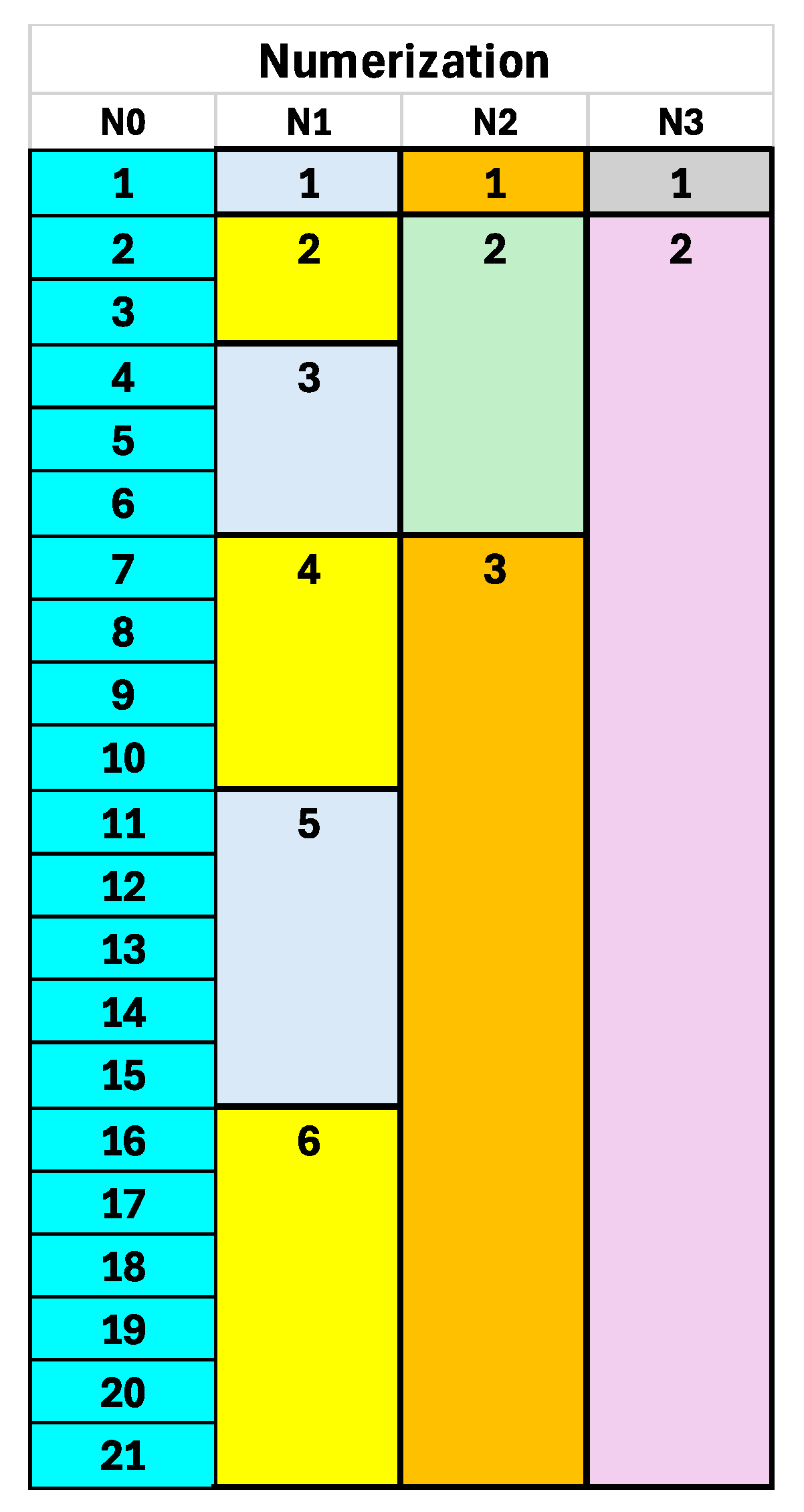
Here below is a graphic representation of four rounds of numerization:(Figure 1)

3. From Distinction to Equivalence

Any two arbitrary numbers x, and y where x ≠ y are distinct. We explore two ways to extract equivalence between them.

1. Approximation, de-specification.

2. De-Approximation, specification

The first method calls for approximating both x and y to such degree that a number a is cast as an approximation of both x and y. The fewer the approximation steps the closer x and y are. Approximation amounts to de-specification, ignoring and removing specificity from both x and y.

The second method is based on the fact that both x and y may be viewed as different approximations of a pre-approximated number p. p was approximated one way from p to x, p → x, and approximated another way from p to y: p → y.

Distinction and equivalence are the essential building blocks for mathematical construction.

4. Approximation & Equivalence

Positive numerization leads to approximation and expanded equivalence, while negative numerization leads to specification and established distinction.

Given a natural number x. By writing it in N1: y_z, one identifies y as the first numerization grade approximation of x. There are x numbers which share same approximation. Say, with the reduced distinction expressed by N1 approximation, one creates an equivalence between two numbers x₁ and x₂, written as x₁ = y_z₁, and x₂ =. y_z₂.

Positive numerization, then, may be regarded as approximation, creating equivalence.

Any arbitrary number x_i = x_i+1_x’_i, obeys: x_i+1 ≤ x_i where the equality only applies for x_i = 1. Accordingly any arbitrary number x > 1 will eventually be approximated to: 2_1_1_1... Hence any two numbers x and y will become equivalent after t rounds of positive numerization.

Example: x = 247837, y = 8976435

We write:

247837 = 704_381 = 38_1_381 = 9_2_1_381 = 4_3_2_1_381= 3_1_3_2_1_381 8976435 = 4237_2469 = 92_51_2469 = 14_1_51_2469 = 5_4_1_51_2469 = 3_2_4_1_51_2469

It takes 5 numerization rounds to achieve equality. We write:

247837 N5 = 8976435 N5

But if we compare y to z = 6784113 then we write: 6784113 = 3684_27 = 86_29_27 = 13_8_29_27 = 5_3_8_29_27 8976435 = 4237_2469 = 92_51_2469 = 14_1_51_2469 = 5_4_1_51_2469

Recording a proximity of degree 4: 8976435 N4 = 6784113 N4

Given two arbitrary numbers x and y expressed in Numerization Nr:

x_r_x_r-1_ ..... _x₁ y_r_y_r-1, ..... _y₁

where x_r = y_r, we then regard |x_r-1 - y_r-1| as the 1st approximate distinction between x and y. and in general, we regard:

|(x_r-1 x_r-2...x_r-i) -(y_r-1 y_r-2...y_r-i) |

As the i-th approximate distinction between x and y.

Approximation establishes equivalence by becoming blind to distinctive details.

5. Specification & Distinction

Numerization implies specification and distinction upon adding a right side number to the underscore tuple.

We have seen that given two arbitrary numbers x and y expressed in Numerization Nr:

x_r_x_r-1_ ..... _x₁ y_r_y_r-1, ..... _y₁

where x_r = y_r, we regard

|(x_r-1 x_r-2...x_r-i) -(y_r-1 y_r-2...y_r-i) |

As the i-th approximate distinction between x and y.

We may apply this distinction over negative numerization much the same. So given two indistinct numbers x=y, we can build a distinction between them as x_i and y_j. where i ≠ j. and 1 ≤ i,j ≤ x=y. We say then that x_i and y_j are first degree distinct.

If i=j, then there is no distinction between x_i and y_j. However we can write x_i_k and y_j_l where k ≠ l. and 1 ≤ k,l ≤ x_i=y_j. We say then that x_i_k and y_j_l are 2nd degree distinct.

And similarly we can establish fine distinctions between otherwise indistinct numbers.

6. Equivocation

The number y = x_ש is interpreted as a number that can be 0.5x(x-1)+1, 0,5x(x-1)+2, .... 0.5x(x-1)+x. This is an extension of the notion of qubit. Equivocation can be extended:

z = x_ש_ש = y_ש,

so z is equivocated over t numbers:

t = Σ_i (0.5x(x-1)+i) = 0.5x²(x-1) + 0.5x(x+1) = 0.5x(x²+1)

With equivocation growing exponentially for: $\mathrm{w}\mathit{=}\mathrm{x}\mathit{\_}{\mathit{ש}}_1\mathit{\_}{\mathit{ש}}_2\mathit{\dots }\mathit{\dots }{\mathit{ש}}_{\mathit{r}}$

The equivocated numbers are consecutive and range from x+1 to x+t. Such equivocation numerization creates a range of arbitrary height for every x. Given two arbitrary numbers x, and y such that y > x, then x can be equivocated through t_x rounds and y can be equivocated through t_y rounds leading for the two equivocation ranges to overlap. There will be n arbitrary numbers z₁, x₂, ... x_n where the x-equivocation range and the y-equivocation range overlap, where n may be made as large as desired, by increasing the values of t_x and t_y.

Example: let x= 3 for t_x=2 the equivocated numbers are:7,8,9.10,...21. Let y=4. for t_y=1 the equivocated numbers are: 7,8,9,10. n=4 numbers overlap.

Computers which can handle computations with such equivocated entities may benefit from this framing of natural numbers.

7. Arithmetic

Nominal arithmetic can be readily extended to numerized expressions. Given two arbitrary numbers x and y expressed in Numerization Nr:

x_r_x_r-1_ ..... _x₁ y_r_y_r-1, ..... _y₁

we will define Nr operations (addition, subtraction, multiplication, division, power raising) involving two Nr numbers resulting in an Nr number.

For y_i = 0 for i=1,2,...r. (0_0_..._0) we write x = x + y, and for y_i = 1 for i=1,2,....r (1_1_1...._1) we have x = y*x = x/y.

Nr numerization addition of x and y: z = x + y. Nr:

z_i = x_i + y_i ....for i=1 to rt

7.1. Addition/Subtraction

Given two arbitrary numbers x and y expressed in Numerization Nr:

x_r_x_r-1_ ..... _x₁ y_r_y_r-1, ..... _y₁

we will define Nr numerization addition of x and y: z = x + y. Nr:

We first normalize both x, and y. Normalization ensures that for x_i_x_i+1, we have: x_i ≤ x*_i+1. where:

x*_i+1 = (x_r_x_r-1_.....x_i+2_x_i+1)

Namely x*_i+1 represents the N0 expression of the tuple x_r...,,,x_i+1 We set:

z_i = x_i + y_i ....for i=1 to r

Note that:

x + y N0 < x +y N1 < x+y N2.....

Example: 5768 + 9823 = 15591

For N1 we write: 5768 = 197_7; 9823 = 140_93. Hence: z₀ = (197+140)_(7+93) = 337_100 = 56716.

For N2 we write: 5768 = 20_7_7l. 9823 = 17_4_93. Hence. z₀ = (20+17)_(7+4)_(71+93) = 37_11_164 = 677_164 = 228990

For r=0,1,2 respectively we have 5768 + 9823 =. 15591, 56716, 228990

Subtraction: Subtraction is defined opposite to addition: Given two arbitrary numbers x and y expressed in Numerization Nr: we first normalize x and y as defined above, (with the MOD’ function) yielding the normalized tuples:

x_r_x_r-1_ ..... _x₁ y_r_y_r-1, ..... _y₁

we will define Nr numerization subtraction of x and y: z = x - y. Nr:

z_i = x_i - y_i ....for i=1 to r

This definition is straight forward as long as x_i > y_i for i=1,2....r

Otherwise we need more mathematical definition.

Zero: Introducing the notion of zero. (0). Zero was described as the state in which “1” rose. It stands mentally to represent ’nothing’. Nothing cannot be properly represented because any representation will amount to something. Nothing is a limiting state of having as minimum as possible of anything. We will use the symbol zero to represent this limiting nothing.

Accordingly:

0 = 0_0_0_.....

0_n = 0_0_0_0...._0_n =n

n_0 = n_0_0....._0 = n

for n ≠ 0.

Thus: x - x Nr = 0_0_.....0 = 0. (a tuple of r underscores).

Negative Natural Numbers: We build a symmetric twin for the list of natural numbers: 1, 2,3, ... marked as -1,-2,-3... and placed in a symmetric fashion with the symbol zero in between:

-n, -(n-1), ...... -3, -2, -1 0 1, 2, 3, .... (n-1), n

The symmetric twin (negative natural numbers) is operated on the same as the positive integers (ignoring the minus sign), but when done, the minus sign is attached.

We denote the numerization of the negative numbers as, N-1, N-2,....

By definition x Nr - x N-r = 0.

x_i - x-_i = 0 for i=1,2,...r

Subtraction is carried out from left to right as follows: if sign = x_r - y_r. > 0 then z = x-y is a positive integer. If sign < 0 then z is a negative integer. If sign = 0 then x_r and y_r are ignored and x and y are treated as N (r-1) numerizations:

x_r-1_x_r-2_ .... x₁ y_r-1_y_r-2_ .... y₁

Normalization should be followed. including negative number. Example: 3_5 = 3_2, 3_-8 = 3_1

As defined x_r and y_r determine if z is positive integer or negative integer.

Example:

x = 459 = 30_24 = 8_2_23

y = 244 = 22_13 = 7_1_13

Both x and y are normalized since (8_2) > 23, and (7_1) > 13. so z = 1_1_10 N3 = 0_1_10 = 1_10 → normalizing = 1_1 = 1

Now we try with y =1500 = 55_15 = 10_10_15

sign = x₃ - y₃ = 8-10 = -2, which is < 0 therefore z < 0

We now subtract (8_2_23) - (10_10_15). We concluded z₃ = -2. z₂ = 2-10 = -8, normalizing over z₃ = -2 we have x₂ = -2. z₁ = 24-15 = 9, normalizing over (-2_-2) = 3 we get z₁ = 1. Hence: z = -2_-2_-1.

7.2. Multiplication/Division

Given two arbitrary numbers x and y expressed in Numerization Nr:

x_r_x_r-1_ ..... _x₁ y_r_y_r-1, ..... _y₁

we will define Nr numerization multiplication of x and y: z = x * y Nr:

z_i = x_i * y_i..... for i=1,2,...r

And normalization of the resultant z tuple.

Example:

x = 459 = 30_24 = 8_2_23

y = 244 = 22_13 = 7_1_13

Both x and y are normalized since (8_2) > 23, and (7_1) > 13.

z = (8*7)_(2*1)_(23*13) N3 = 56_2_299 = 1542_299 = 1188410

larger than x * y N0 = 459*244 = 111996

Division: For z Nr which is the multiplication of x Nr over y Nr, we define division as a multiplication-reverse:

y = z/x N3; x = z/y N3

For a general tuple z Nr and x Nr the division y/x is carried on as follows:

Case 1 all y_i = z_i/x_i for i=1,2,..r are integers. In that case

y = y_r_y_r-1_.... y₁

Case 2. For i = r, (r-1), (r-2).....(i+1) y_i = z_i/x_i are all integers while z_i is not an integer for i=r

In this case there are two division options: (i) approximation, (ii) specification.

In approximation we write:

y = y_r_y_r-1_.... y_i_0_0...._0

In specification we write:

*z_i = z_r_z_r-1_.... z_i_ ש

*x_i = x_r_x_r-1_.... x_i_ ש

And we seek to replace the two ש ’place holders’ with z_i and x_i such that y_i = z_i/x_i is an integer. If no such two specification numbers can be used to replace the שs then, we extend another ש and write:

*z_i = z_r_z_r-1_.... z_i_ש_ש

*x_i = x_r_x_r-1_.... x_i_ש_ש

and try all possible ש options to find y_i = z_i/x_i as an integer. If no such four specification numbers can be used to replace the שs then, we extend another ש and keep the extension until y_i is an integer.

And then continue with z_j and x_j to set y_j and on for j= (i-1), (i-2), ..... 1

Example: z = 12_4_18, x = 3_4_3:

y N2 = (12/3)_(4/4)_(18/3) = 4_1_6 = 7_6 = 27 N0

while for z = 12_4_18 = 70_18 = 2433 N0. And x = 3_4_3 = 7_3 = 24 N0 we write:

y N0 = (z N0) /(x N0) = 2433/24 = 101.375

But for x N3 = 3_4_5 we have:

y N3 = (12/3)_(4/4)_(18/5)

Since 18/5 is not an integer we may choose the approximation method:

y N3 -- Approximation = (12/3)_(4/4) = 4_1 = 7

Or we may use specification. method:

z = 12_4_18_ש x = 3_4_3_ ש

We write:

z = 2433_ש, x = 24_ ש

We write:

z = 2433_109 = 2958637

x = 24_1 = 277

y = z/x = 2958637/277 = 10681

7.3. Power Raising

Given arbitrary x in Nr taken in normalized form:

xr_xr-1_ ..... _x1

It can be raised by a power p Nr taken in normalized form:

pr_pr-1_ ..... _p1

y = x^p Nr where: y_i = (x_i)^p_i.

Example: x N2 = 23_4_11 = 257_11 = 32907

p N2 = 2_2_1 = 3_1 N2 = 4

y = xp = (232)_(42)_(111) = 529_16_11 = 139672_11 = 9754063967

while y = x^p N0 = 32907⁴ = 1172608842465681201

Root Extraction: Given that y = x^p, we can say that x = y^1/p. In general root extraction will be handled just like division, ensuring an integer based on one of the two formerly discussed methods: approximation or specification.

8. Numerized Arithmetic

Variables and coefficients used in algebraic expressions can each be written in any non-negative numerization, Nr. Addition, subtraction, multiplication, division, power raising, root extraction are all well-defined for the various numerized expressions of integers. So one could manipulate symbols, calculate and process integers in any arbitrary numerized expression. This includes solving algebraic arithmetic questions.

Furthermore one could, at any point, switch numerized representation from some value Ni to some value Nj where i ≠ j, and then to Nk where k ≠ i, k ≠ j. An algebraic operation o₁ can be done with numerization r₁, then one may switch to numerization r₂, then one may continue to process with operation O₂, followed by a switch to numerization level r₃, and so on. The result will depend on the shift pattern between numerization levels.

Example: y = f(x) = 3x² + 2x + 4

Compute y = f(x) N0 for x=2:

y = 3*2²+2*2+4 = 20

Compute y=f(x) N1 for x=2

y N1 = (2_2)*(2_1)^(2_1) + (2_1)*(2_1)+(3_1)

= (2_2)*(4_1) + (4_1) + (3_1) = (8_2) + (4_1) + (3_1) = (15_4) = 109

Multi Level Arithmetic An arbitrary number x Nr may be readily mapped to x Np for any p ≠ r. A given set of n variables V₁, V₂, ..... V_n Nr may be operated on in Nr (O_r) to generate a set of m variables U₁, U₂, ..... U_m Nr. These m variables may then migrate to Np and be operated on with operation O_p to generate a set of q variables W₁, W₂, ..... W_q Np. And so on, operation after operation where each successive operation operates on a different numerization level.

Such numerization migration defines a multi level arithmetic. It defines an operational wealth for which the common arithmetic is a collapsed version.

Much as arithmetic abstracts itself to algebra so does multi-level arithmetic abstracts itself to multi-level algebra.

Numerized Functional Relationships

Let X and Y be two arbitrary integers in Nr. x = x_r_x_r-1_ ..... _x₁ Y = Y_r_Y_r-1_ ..... _Y₁ . We may identify a variety of functional relationships between X and Y. For example: MAX, MIN, MOD.

Illustration: Let X = 12_4_7 and Y=8_14_3. We write:

Z = X MAX Y = (12_4_7) MAX (8_14_3) = 12_14_7

We also write:Z = X MOD Y = (12_4_7) MOD (8_14_3) = (4_4_1)

9. Attributes

Numeric attributes common with N0 can be extended to Nr. We discuss, primes, composites, multiplications, fractions, as well as more esoteric attributes like uniform numbers and perfect numbers.

9.1. Primes

An arbitrary number x Nr where at least for some i=1,2,...r. x_r is prime is regarded as “Base prime”. since there is no y Nr number for which y_i > 1 for i=1,2,...r. such that x/y is an integer.

A base prime Nr may be a composite number for Np for p < r. Example: x = 7_5_3 N2 (prime) = 26_3 N1 (prime) = 328 N0 (composite).

An arbitrary number x Nr where for all i=1,2,...r. x_r is prime is regarded as “Full Prime”. since there is no y Nr number for which y_i > 1 for which any x_i/y_i is an integer for any i=1,2,...r

9.2. Composites

An arbitrary number x Nr where for i=1,2,...r. x_r is composite is regarded as “Nr Composite” since there are one or more y Nr numbers for which y_i > 1 for i=1,2,...r. such that x/y is an integer Nr.

Example: Let x = 6_9_15. We have:

for y = 2_3_5. x/y = (6/2)_(9/3))_(15/5) = 3_3_3.

9.3. Uniform Numbers

A number x Nr is considered uniform for x’ if and only if x’ = x_i for i=1,2,...r.

The series of uniform numbers is: 0_0_0, 1_1_1, 2_2_2, 3_3_3, 4_4_4,.... N2

which are: 0, 1, 5, 18, 49, N0

9.4. Fractions

Writing two Nr numbers, x, y, in fraction form, defines thereby a fraction, f_xy

x_r_x_r-1_ ..... _x₁ y_r_y_r-1, ..... _y₁

f_xy = (x_r_x_r-1_ ..... _x₁)/ (y_r_y_r-1, ..... _y₁)

10. Applications

Applications involving approximation, specification, and obfuscations are all of interest in the numerized realm. Same for applications where one digs for unseen patterns. Hence numerization appears useful for probability calculus, quantum computing, AI inference. The field is attractive for cryptographic primitives.

10.1. Error Assessment

Given x Nr: x_r_x_r-1, ..... _x₁

Let there be an error in some x_i, which is written as x’_i. where. e = x’_i - x_i.

The higher the value of i, the greater the impact of the error on x N0.

Example: let x = 5_3_3, = 13_3 = 81

let e=1 and i=3 hence x_e = 6_3_3 = 18_3 = 156

An error in x. N0 of 92% while for 5_3_4 = 5_3_1 = 18_1 = 79 An error of 81/79 = 2%

10.2. Numerization Modes

In addition to the standard numerization mode in which each round the leftmost number is numerized, we can apply other modes. In particular: (i) double sided numerization, (ii) centric numerization, and (iii) full line numerization. In the first mode, in each numerization round both the rightmost and the leftmost number are numerized. In the second numerization the two most centric numbers in the tuple are numerized each round. In the third mode each round all numbers are numerized. Once the mode is known, these modes allow for reversal -- restoring the pre-numerization number.

Example: Nominal Numerizatio

7892323817 = 125637_58751 = 501_387_58751 = 32_5_387_58751 = 8_4_5_387_58751 = 4_2_4_5_387_58751

Double side numerization:

7892323817 = 125637_58751 = 501_387_343_98 = 32_5_387_343_14_7

Centric numerization:

7892323817 = 125637_58751 = 501_387_343_98 = 501_28_9_26_18_98 = 501_28_4_3_7_5_18_98

Full Line numerization

7892323817 = 125637_58751 = 501_387_343_98 = 32_5_28_9_26_18_14_7

10.2.1. Variations

Numerization may be explored through a series of variations. We mention here shift numerization, split numerization, circular numerization. Shift numerization is the situation where the counting shifts from 1,2,3,.... to some number n, n+1, n+2, for n > 1. Split numerization refers to selecting an arbitrary point as ’zero’ and applying positive numerization to its right and negative numerization to its left. Circular numerization describes numerization over a modular ring of integers.

10.2.2. Binary Strings Numerization

Numerization can be used to write binary strings differently, for any prospective purpose.

Consider the following binary string:

x = 11001100111011000110111100101001110110101011110

Its numeric value is: x = 20303025270 which can be Numerized in the full front method:

x = 20303025270 = 201509_187484 = 635_214_612_518

Onward:

x = 36_5_21_4_35_17_32_22 = 8_8_3_2_6_6_3_1_8_7_6_2_8_4_7_1

This string can be expressed using binary alphabet by writing every one of the 16 numbers above through a unary alphabet flipping between the bits identity. So we start with 8 zeros followed by 8 “ones” followed by 3 zeros, etc:

x =00000000111111110001100000011111100010000000011111110000001100000000111100000001

The above string is content identical to the original x string

Alternatively, given that the numerization proceeded such that 8 is the largest number, one can express this numerization by a series of 3 consecutive bits, per each numerization number. Since 0 is excluded from the numerization, we express the series, 8_8_3_2... as 000 000 011 010.. which computes to:

x = 00000001101011010011001000111110010000010111001

The above string also is of the same content as the original string x (bijection)

10.3. Estimation

When x represents a measurement, or a calculation of a well-defined value. There may be a difference between the ’true’ value one tries to measure or calculate, x^, and x. But when both x and x^ are numerized then x_i is more likely to coincide with x^_i, the higher the value of i.

Example. Let x^ = 50 and x = 46 , we write x^ = 50 = 10_5, and x= 46 = 10_1 We see that

x₂ = x^₂ = 10

We therefore can reduce 10_5 to 10_ש to indicate that x₁ in the measurement or calculation are of too low validity, and should not qualify as data. We can then replace the ש with the top of the x₁ range, the bottom, or the middle, per an arbitrary decision. (Note: nominally the middle range is best, it has the shortest distance from the unknown true value. For even count select top or bottom). And then we use this choice in rewriting x. So instead of x=46 we write x = 10_6 = 51.

To express even greater doubt about the accuracy of the measurement or calculation we may go to N2:

46 = x₃_x₂_x₁ = 10_1 = 4_4_1

And write x = 4_ש_ש. Similarly. x^ = 4_4_5

Now writing x = 4_4_10 =55

A more common approach uses the negative numerization to chart a range. For numerization level N-1 we write x = x₂_ש, and replace ש once with 1 and once with x₂ to define a range.

In the example above it figures as a range from 10_1 to 10_10, namely: 46-55, which includes x’

10_1. ≤ x’ ≤ 10_10 Namely: 46 ≤ x’ ≤ 55

If we are less confident about our measurement we will go down to N-2: x = x₂_ש_ש, and again define the range between the lowest possible values for ש and the highest.

Writing the measurement x as x = 46 = 10_1 = 4_4_1 = 4_ש_ש, we identify the bottom of the range: 4_1_1 = 22, and the top of the range: 4_4_10 = 55, writing 22 ≤ x’ ≤ 55

The same may apply to N-3, N-4, etc.

10.4. Non-Linear Addition, Multiplication.

In quite a few situations the linear addition z = x + y is non-reflective of reality. At times z should be larger than the linear addition, and at times smaller, same for multiplication. When adding risk for example, combined risk if larger than linear add-on, in adding probabilities, a range of overlapping cases will result in a lower probability than linear add on. Numerization arithmetic can readily be used to express such non-linear situations.

Given z = x + y. N0, one may map, x, and y to N1: x₁_x₂, y₁_y₂, and add: z = x + y N1. and then map z N1 to (z N1) N0, where (z N1) N0 > z N0. This non-linearity may be extended at will by choosing a higher numerization level i:

(z Ni) N0 > (z Nj) N0 for i > j

Example: z = x + y; x = 54. y = 85. z = 139.

We write: 54 = 10_9, 85 = 13_7 and so z = (10+13)_(9+7) = 23_16 = 269

Indeed 269 > 139.

Going further to N2: 54 = 4_4_9; 85 = 5_3_7 and so z = (4+5)_(4+3)_(9+7) = 9_7_16 = 43_16 = 919

So the N0 mapping of z N2, z N1, z N0 is 919, 269, 139

For situations where the nonlinearity is in the opposite direction, to suppress the outcome, one would treat x and y as the x₂ and y₂ values respectively of negative numerization expansion N-1: x’ = x₂_x₁, and N-1 y’ = y₂_y₁ where x₁ = y₁ = ש. Given that 1 ≤ x₁ ≤ x₂, one can choose any value within this range, nominally -- the top of the range, so x₁ = x₂, and similarly y₁ = y₂ .

And to increase the suppression one might map x and y in N0 to x₂_ש_ש and y₂_ש_ש, and so on. In general:

(z N-i) Nj < z N-j. for i,j=1,2,... and i > j

Example: z = x + y; x = 54. y = 85. z = 139.

We write. x N0 = 54_ש, y N0 = 85_ש, becoming x N0=54_54, and y N0=85_85

Mapping (x N0) N-1 = 54_54 = 1485. And mapping (y N0) N-1 = 85_85 = 3655

And hence z N-1 = (x N0) N-1 + (y N0) N-1 = 1485 + 3655 = 5140

Further. (z N-1 ) N0 = 5140 N-1 = 101_90

which becomes 101_ש, converting to 101 which is smaller than x+y = 139

Going for N-2, x, and y are written as: x₂_ש_ש, and y₂_ש_ש, where we replace the ש with the top of the range: x N0 = 54_54_1485 and y N0 = 85_85_3655, and the corresponding numbers at N-2 are:

54_54_1485 = 1485_1485 = 1103355 = x N-2

85_85_3655 = 3655_3655 = 6681340 = y N-2

And so:

z N-2 = 1103355 + 6681340 = 7784695

for which the corresponding N0 is: 89_30_1210 = 89_ש_ש .

So in summary x+y plain (N0), N-1, N-2 values are: 139, 101, 89

Similarly for multiplication both expansion and contraction option are numerization enabled.

10.5. Re-Anchoring

Numerization may be re-anchored anywhere on the original list of natural numbers. Anchor A means that A+1 is the integer deemed as 1 for numerization process, A+2 is integer 2, A+i integer i, and A is represented by the 0 indication in numerized vocabulary.

Everything that takes place in pre-anchoring numerization has a corresponding event in anchored representation.

There is a clear mapping between any numerized tuple before anchoring and after anchoring as well as between two different anchored designations.

Example: x = 111, Pre-anchoring x N1 = 15_6. Let A = 48, namely x N0 (A=48) = 63 N0 (A=48) so: x N1 (A=48) = 11_8, and similarly:

Pre A 15_7 = 11_9 (A=48).Pre A 15_8 = 11_10 (A=48)Pre A. 15_9 = 11_11 (A = 48)Pre A. 15_10 = 12_1 (A=48)

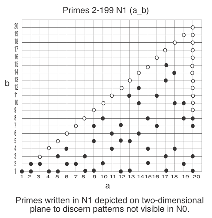
10.6. Pattern Recognition

Let there be n measurements. x₁, x₂, ..... x_n, of n items, each with respect to a particular attribute of the items. And let there be m measurements of the same attribute of different m items y₁, y₂, ..... y_m. The n first items belong to a category X and the m latter items belong to a category Y. One tries to find a discriminating pattern between the two categories so that given another measurement z , one will be able to state with some confidence whether the z measured item belongs to category X or category Y.

This cluster analysis is normally done over the nominal measured values, all in N0. However, mapping these n+m+1 measurements each to Nr will offer the pattern analyzer a much richer domain in which to discern pattern. The Nr expression of the measurements will depict the n+m+1 cases as n+m+1 points on an r-dimensional space exposing clusters not visible with N0.

This enhanced pattern recognition is widely applicable. For fractional measurement, a multiplication by all denominators will yield natural numbers that are readily numerized.

Example, for measurement. 1.44, 0.28, 1.11, multiplying x100 yields: 144, 28, 111.

The numerization born pattern recognition may also be used to find profound mathematical attributes like prime numbers.

11. Analysis

This numerization construction is faithful to the unmatched clarity of natural numbers, a succession of distinction -- the foundation of mathematics. It stops short of the common extension to irrational numbers, continuity, infinity, motion. This extension is well handled by mathematical formalism, but at the cost of the conceptual clarity that is claimed by the natural numbers.

Historically the battle between the discrete and the continuous was raging for centuries, either notion regards the other as an approximation. A no lesser authority than David Hilbert asserted:

“Our First Naive impression of Nature and matter is that of continuity. Beit a piece of metal or a volume of liquid, we invariably conceive it as divisible into infinity.”

It stands to reason to explore mathematics from either direction. This thesis does so from the side of natural numbers, with numerization offers them a new wealth of expression to handle situations more naturally handled through continuity, irrationality, infinity.

The main interest in numerization is its aspect of novelty regarding the fundamental entities of mathematics: the series of natural numbers. They harbor secret, patterns, relationships which are still hidden from the common knowledge of mathematics. Any novel method that writes and manipulates these natural entities with minimum arbitrariness and maximum naturalness is of interest because of its potential to reveal numeric properties not yet known.

Numerization keeps its analysis in the realm of natural numbers, avoiding the ’continuity trap’ that leads to irrational numbers. It introduces two opposing complimentary concepts: approximation and specifications with which it meets the known limitations of integers normally solved with irrational numbers, and qubits.

The numerization concepts presented herein appears qualified for further investigation by the community at large, and to their attention this piece is addressed.

References

- Dantzig, Tobias “Number -- The Language of Science”. 4th Edition, The Free Press, 1954.
- Waismann, F., Introduction to Mathematical Thinking, Harper Torchbooks, New York, 1959.
- Benacerraf, P., “What Numbers Could Not Be,” Phil. Rev., vol. LXXIV, 1965, pp. 47–73. [CrossRef]
- Sich Jeffrey, “ Counting and the Natural Numbers” Philosophy of Science , Volume 37 , Issue 3 , September 1970 , pp. 405 - 416. [CrossRef]
- Helmut Hasse, “Number Theory”. Feb 2022 · Walter de Gruyter GmbH & Co KG.
- Trygve Nagell “ Introduction to Number Theory” AMS Chelsea Publishing: July 2021.
- G. Samid “ Negotiating Darwin’s Barrier: Evolution Limits Our View of Reality, AI Breaks Through”. https://www.preprints.org/manuscript/202409.1505/v1.
- Innovation Solution Protocol, www.InnovationSP.net.
- G. Samid, “Metaverse Oriented Geometry” https://www.researchgate.net/publication/360084946_Metaverse_Oriented_Geometry.
- G. Samid “Artificial Intelligence Assisted Innovation” 2023 https://www.intechopen.com/chapters/75159.
Disclaimer/Publisher’s Note: The statements, opinions and data contained in all publications are solely those of the individual author(s) and contributor(s) and not of MDPI and/or the editor(s). MDPI and/or the editor(s) disclaim responsibility for any injury to people or property resulting from any ideas, methods, instructions or products referred to in the content. |
© 2025 by the authors. Licensee MDPI, Basel, Switzerland. This article is an open access article distributed under the terms and conditions of the Creative Commons Attribution (CC BY) license (http://creativecommons.org/licenses/by/4.0/).
Copyright: This open access article is published under a Creative Commons CC BY 4.0 license, which permit the free download, distribution, and reuse, provided that the author and preprint are cited in any reuse.