Submitted:
28 February 2025
Posted:
03 March 2025
You are already at the latest version
Abstract
Intracranial aneurysm is a common clinical disease that seriously endangers the health of patients. In view of the shortcomings of existing intracranial aneurysm recognition methods in dealing with complex aneurysm morphologies, varying sizes, as well as multi-scale feature extraction and lightweight deployment, this study proposes an intracranial aneurysm recognition method named AS-YOLO to improve the detection accuracy of intracranial aneurysms and adapt to the deployment on lightweight devices. This algorithm is based on the basic framework of YOLOv8n. Firstly, a cascaded fusion network is constructed to enhance the multi-scale feature extraction ability. Secondly, a multi level feature fusion module is designed to achieve more efficient multi-scale feature fusion. Then, the detection head is improved by proposing an efficient depthwise separable convolutional detection head , which reduces the number of model parameters and computational complexity while maintaining the detection accuracy. Finally, the SIoU loss function is introduced to make the bounding box regression of the model more accurate and further improve the detection performance. Compared with the original YOLOv8, the model proposed in this paper not only improves the detection accuracy in the aneurysm recognition task, with the mAP0.5 increased by 8.7% and the mAP0.5:0.95 increased by 4.96%, but also significantly reduces the number of model parameters and computational complexity, with the parameter quantity decreased by 8.21%. The model proposed in this paper combines multi-scale feature fusion and lightweight design, and can effectively meet the application requirements in resource-constrained environments such as mobile healthcare while ensuring high detection accuracy.
Keywords:
YOLOv8
; Aneurysm Recognition
; Multi-scale Features
; Cascaded Fusion Network
; Lightweight
1. Introduction
Intracranial aneurysms are abnormal dilations of cerebral artery walls, often caused by congenital weakness or acquired damage, with a prevalence of approximately 3% [1]. They are a major cause of subarachnoid hemorrhage [2]. Aneurysm rupture can be life-threatening, with a mortality rate reaching 32% [3]. After the first rupture, 8% to 32% of patients may die, with a disability and mortality rate exceeding 60% within one year and reaching 85% within two years [4,5]. Therefore, early diagnosis and treatment are crucial. Current diagnostic methods for intracranial aneurysms include computed tomography (CT), digital subtraction angiography (DSA), CT angiography (CTA), and magnetic resonance angiography (MRA), with DSA widely recognized as the gold standard [6]. However, manual analysis of DSA images is time-consuming, and the high workload of radiologists may lead to delays. Additionally, small or morphologically complex aneurysms are more prone to misdiagnosis or missed detection due to the limitations of subjective judgment.
Intracranial aneurysm detection algorithms are mainly categorized into traditional and deep learning-based methods. Traditional approaches rely on aneurysm feature detection. For example, Rahmany et al. [7] used the maximally stable extremal regions (MSER) algorithm to extract vascular structures from DSA images and employed Zernike moments and the MSER detector to identify aneurysms. However, due to the complexity of aneurysm morphology and location, traditional algorithms have limited generalization ability.
In recent years, deep learning has demonstrated outstanding performance in medical image analysis, making it an important tool for assisted diagnosis. The application of convolutional neural networks (CNNs) has driven the automation of intracranial aneurysm detection. Nakao et al. [8] proposed a detection method combining CNN with maximum intensity projection (MIP), while Claux et al. [9] adopted a two-stage regularized U-Net [10] for MRI-based aneurysm detection, achieving good results but with high computational costs. Mask R-CNN [11] has shown excellent performance in medical image analysis but is computationally complex, making real-time detection challenging. TransUNet [12], which integrates Transformer and U-Net, enhances the detection of small aneurysms but requires substantial computational resources, limiting its application in low-power devices. Therefore, while CNNs and their variants perform well in medical image detection, their high computational complexity remains a challenge for real-time detection and lightweight deployment.
In the field of general object detection, the YOLO series algorithms have gained widespread attention due to their efficient end-to-end detection performance. Qiu et al. [13] successfully utilized YOLOv5 to predict the bounding boxes of intracranial arterial stenosis in MRA images, demonstrating the feasibility of the YOLO series in medical image analysis. However, in the task of intracranial aneurysm detection, YOLO-based algorithms still face several challenges: (1) Limited multi-scale feature fusion capability, making it difficult to detect small or morphologically complex aneurysms. (2) High computational cost, restricting deployment on embedded devices or low-power computing terminals.
To address these challenges, this paper proposes AS-YOLO, a lightweight intracranial aneurysm detection algorithm based on YOLOv8n, which is specifically optimized for aneurysm detection. The main contributions of this work are as follows:
(1)Improved Cascade Fusion Network (CFNeXt): To enhance multi-scale feature fusion capability, this paper introduces the CFNeXt network, which replaces the C2F module in the YOLOv8 backbone with an improved CFocalNeXt module. This modification generates more hierarchical feature representations, improving the recognition of aneurysms of varying scales.
(2)Multi-Level Feature Fusion Module (MLFF): To address the limitations of YOLOv8 in feature fusion, MLFF employs 3D convolution and scale-sequence feature extraction, integrating high-dimensional information from both deep and shallow feature maps. This significantly enhances feature fusion effectiveness, particularly in the detection of small aneurysms.
(3)Efficient Depthwise Separable Convolution Head (EDSA): The multi-level symmetric compression structure in the YOLOv8 detection head has limitations in flexibility. This paper proposes the EDSA detection head, which allows for more adaptable processing of diverse feature representations and aneurysm size distributions, thereby improving detection speed while reducing computational overhead.
(4)Improved SIoU Loss Function: To address the slow convergence issue of CIOU Loss in the regression process, this work introduces the SIoU loss function. By considering the angular vector between the predicted and ground truth bounding boxes, SIoU enhances bounding box alignment precision and accelerates training convergence.
Experimental results demonstrate that the proposed AS-YOLO model achieves significant improvements in multi-scale feature fusion, computational efficiency, and model lightweighting. Compared to YOLOv8, AS-YOLO improves accuracy by 3.51%, increases mAP50 by 8.7%, and reduces the number of parameters by 8.21% on the DSA intracranial aneurysm dataset, achieving a balance between detection accuracy and lightweight deployment.The next section will provide a detailed description of the AS-YOLO algorithm’s foundation and innovations.
2. Materials and Methods
2.1. Baseline Method-YOLOv8
YOLOv8n (You Only Look Once v8-nano), released by Ultralytics in January 2023, is designed specifically for efficient object detection tasks. It inherits the core principles of the YOLO series [14,15,16,17,18,19,20], which emphasize fast and accurate object detection through a single-stage network structure. Compared to previous versions like YOLOv5 [21] and YOLOv7, YOLOv8n incorporates various improvements in network architecture, feature extraction, and efficiency optimization, making it especially suitable for edge devices and real-time detection scenarios, such as mobile devices or embedded systems.
The core architecture of YOLOv8n retains the “end-to-end” approach typical of the YOLO family, performing both object classification and bounding box regression in a single forward pass. The network consists of three main parts: Backbone, Neck, and Head. The Backbone network extracts basic features from the input image; the Neck network fuses multi-scale features; and the Head is responsible for predicting the class and location of objects.
The Backbone uses CSPDarknet [22] as its main structure, with CSPLayer_2Conv modules as fundamental units. Compared to YOLOv5’s C3 module, the C2f [23] module offers fewer parameters and superior feature extraction capability. Additionally, Bottleneck Block and SPPF modules enhance the feature extraction capacity. The Neck network sits between the Backbone and Head, focusing on feature fusion and enhancement. YOLOv8n introduces an improved feature pyramid structure within the Neck, effectively integrating feature information from different levels. This structure combines the strengths of Feature Pyramid Network (FPN) and Path Aggregation Network (PAN), improving multi-scale feature fusion, particularly for small object detection. This design allows the network to capture both local details and global information, enhancing detection accuracy.
The Head network is the decision-making part of the object detection model. It uses feature maps of various sizes to obtain the object category and location, producing the final detection results. A decoupled head structure is used, including separate detection and classification heads. An overview of the YOLOv8 network architecture is shown in Figure 1.
2.2. Proposed Method
In this study, the YOLOv8n algorithm serves as the foundational model, which has been optimized and enhanced for the DSA intracranial aneurysm dataset, resulting in an improved AS-YOLO model. First, a lightweight Cascade Fusion Network (CFNeXt) is introduced into the Backbone layer, where the CFocalNeXt module replaces the original C2f module, enhancing the model’s multi-scale feature extraction capability and enabling it to more effectively capture features of aneurysms of varying sizes.
Additionally, a Multi-Level Feature Fusion (MLFF) module is employed in the Neck layer to improve the fusion of feature maps at different levels, significantly boosting multi-scale aneurysm detection performance. In the detection head, an Efficient Depthwise Separable Convolution Head (EDSA) is proposed. By applying asymmetric compression to features along different paths, this detection head optimizes feature utilization efficiency, reducing the model’s parameters and computation while enhancing both generalization capability and detection speed.
To further improve detection accuracy and convergence speed, this study also introduces the SIoU loss function, which refines the accuracy of bounding box regression. This adjustment better meets the demand for high-precision bounding box alignment, especially crucial for aneurysm detection tasks. The improved YOLOv8n network structure is shown in Figure 2.
2.2.1. Backbone Network CFNeXt
In aneurysm recognition tasks, the limited capacity for multi-scale feature fusion restricts the model’s ability to identify aneurysms of varying sizes effectively. To address this issue, inspired by the Cascade Fusion Network (CFNet) [24], this study introduces a new Backbone network, CFNeXt, as an improved Backbone structure for YOLOv8, as shown in the table below.

Table 1.
CFNeXt Network Architecture Table
| Index | Module | Input Channels | Output Channels | Stride |
|---|---|---|---|---|
| Stage0 | Conv | 3 | 16 | 2 |
| Stage1 | Conv | 16 | 32 | 2 |
| CFocalNeXt | 32 | 32 | 1 | |
| Stage2 | Conv | 32 | 64 | 2 |
| CFocalNeXt | 64 | 64 | 1 | |
| Stage3 | Conv | 64 | 128 | 2 |
| CFocalNeXt | 128 | 128 | 1 | |
| Stage4 | Conv | 128 | 256 | 2 |
| CFocalNeXt | 256 | 256 | 1 |
The Backbone consists of five parts: Stage0, Stage1, Stage2, Stage3, and Stage4. Stage0 serves as the Conv layer for downsampling at the input of the original image. This Conv layer is composed of a standard convolution, batch normalization layer, and SiLU [25] activation function to perform downsampling.Each of the following stages has two components: the first part is a Conv layer used for downsampling, and the second part is a CFocalNeXt module, which serves as the core module for feature extraction.
The downsampling factors for each part are 2, 4, 8, 16, and 32 times, respectively, while the output channels are 16, 32, 64, 128, and 256, respectively. Finally, the features extracted by the CFNeXt backbone network are fused and passed into the SPPF pyramid pooling structure. The structure of CFNeXt is shown in Figure 3.
In complex scene detection tasks, multi-scale object detection has always been a significant challenge. A common solution is to generate feature maps at different resolutions. In recent years, researchers have explored global attention mechanisms (such as the Transformer series) or large convolutional kernels (such as the RepLKNet series with a 31×31 kernel [26]) to expand the receptive field. Although these methods have achieved good detection performance, applying such modules in complex scenes still faces great challenges. Due to the large input image size, using these large modules as core feature extraction components incurs high computational costs and memory overhead, increasing the complexity of the detection model.To address this issue, this paper proposes the CFocalNeXt module, which enhances feature representation capability while reducing computational complexity. The CFocalNeXt structure is shown in Figure 4.
The CFocalNeXt module is an improved version of the C2F module. It first employs a standard Conv convolution module to extract feature information from the input feature map and then divides the extracted features into two branches:
- One branch serves as a residual connection, preserving the original information flow;
- The other branch feeds the feature map into the FocalNeXt module to further optimize feature representation.
The FocalNeXt feature focusing module incorporates two dilated convolutions [27] and two residual connections, and it is divided into two parts:
-
Multi-scale Feature Extraction
- A 7×7 convolution is used instead of the traditional 3×3 convolution to enhance local information aggregation capability.
- A depthwise separable convolution with a dilation factor of r=3 expands the receptive field, balancing accuracy and computational cost. Experiments show that r=3 improves accuracy by 2.4% and reduces computational overhead by 5.2% FPS. Increasing r (e.g., r=5) slightly improves accuracy but significantly increases computational complexity.Table 2. Model Performance Under Different Dilation Factors.
Configuration mAP0.5 GFLOPs Params(M) FPS CFocalNeXt(r=1) 0.786 6.8 2.581 103.6 CFocalNeXt(r=3) 0.805 7.2 2.662 98.2 CFocalNeXt(r=5) 0.812 7.5 2.796 94.5
-
Lightweight FFN Structure
- LayerNorm (LN) [29]replaces BatchNorm (BN) [28]to enhance training and inference stability for small batch sizes. Replacing BatchNorm with LayerNorm improves mAP (0.805 vs. 0.793) while maintaining nearly the same inference speed (98.2 vs. 98.1), making it suitable for object detection tasks with varying input sizes.
- GELU activation is introduced between 1×1 convolution layers to enhance nonlinear representation capability.
- Channel expansion (×4) and compression (÷4) mechanisms are applied to reduce computational cost.
Table 3.
Comparison of Model Performance with BatchNorm and LayerNorm
| Configuration | mAP0.5 | GFLOPs | Params(M) | FPS |
|---|---|---|---|---|
| BatchNorm | 0.793 | 7.2 | 2.662 | 98.1 |
| LayerNorm | 0.805 | 7.2 | 2.662 | 98.2 |
In summary, CFocalNeXt improves detection accuracy while maintaining high computational efficiency through multi-scale feature extraction and lightweight structural optimization.
2.2.2. Multi Level Feature Fusion Module
This structure experiences a decline in detection performance when handling excessively large or small objects. To address multi-scale feature fusion challenges, previous studies have explored various approaches:
- Image Pyramid Structure: Constructs an image pyramid and extracts features independently at different scales. Each feature map retains strong semantic information, but there is no interaction between different scales.
- Hierarchical Pyramid Feature Structure(SSD[30]): The backbone network generates multi-scale feature maps, discarding shallow features to reduce low-level interference. However, removing high-resolution features negatively impacts small object detection.
- Feature Pyramid Network (FPN) [31]: Utilizes a top-down structure with lateral connections to fuse high-resolution low-level features with semantically rich high-level features.
- Path Aggregation Network (PANet) [32]: Builds upon FPN by introducing bottom-up path aggregation to address the limitation of one-way information flow, enhancing feature fusion and improving small object detection.
Figure 5.
Comparison of FPN and PANet Network Structures. (a) FPN architecture. (b) PANet architecture.
Figure 5.
Comparison of FPN and PANet Network Structures. (a) FPN architecture. (b) PANet architecture.
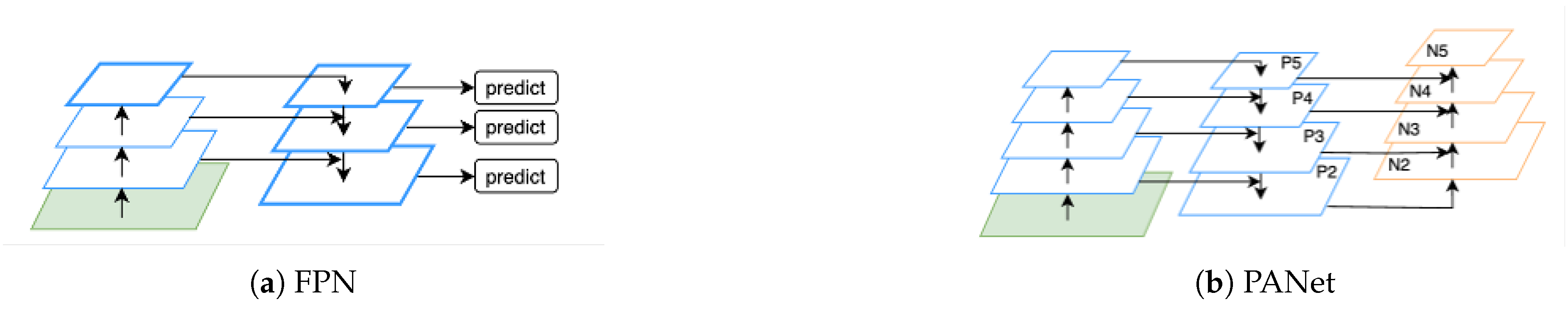
YOLOv8 adopts the PANet structure for feature fusion, but since it only uses concatenation, it does not fully consider feature interactions, limiting its performance in densely overlapping small object detection tasks. Inspired by ASF-YOLO [33], this paper proposes the Multi-Level Feature Fusion Pyramid Network (MFFPN), which enhances the PANet structure by replacing simple concatenation with multi-level feature fusion. To improve the detection performance of densely overlapping small objects, we design the Multi-Level Feature Fusion (MLFF) module (as shown in Figure 6), which integrates feature information from P2/P3, P4/P3, P4, and P5, corresponding to outputs of different scales.
- For large-sized feature maps, the channel count is adjusted to 1C after being processed by the Conv module to ensure a smaller proportion in concatenation operations without affecting subsequent learning. Then, a max pooling + average pooling structure is used for downsampling, reducing the spatial dimension of features while achieving translation invariance, thereby enhancing the network’s robustness to spatial variations and translations in the input image. From the table below, it can be seen that using a hybrid pooling strategy achieves higher accuracy (mAP0.5) compared to using max pooling or average pooling alone, while maintaining nearly the same computational cost, thereby improving detection performance.Table 4. Experimental Performance of Different Pooling Strategies
Pooling Strategy mAP0.5 GFLOPs Params(M) FPS Max Pool 0.784 8.1 3.020 86.4 Avg Pool 0.781 8.0 3.000 86.7 Max+Avg(Ours) 0.788 8.3 3.0572 85.2 - For small-scale feature maps, we first use a Conv module to adjust the number of channels and then apply the nearest neighbor interpolation method [34] for upsampling. Compared to other upsampling methods, nearest neighbor interpolation has the advantages of low computational cost and high speed, making it more suitable for embedded deployment. In our experiments, our method maintains low computational overhead and parameter count while achieving an inference speed of 85.2 FPS, significantly outperforming the other two methods. Although transposed convolution and attention-guided upsampling show slight improvements in mAP0.5, their computational costs (9.5 GFlOPs and 10.1 GFlOPs, respectively) and inference speed reductions are notable. Therefore, considering accuracy, computational cost, and inference efficiency, the nearest neighbor interpolation method maintains detection accuracy while offering superior computational efficiency and balance, making it a more suitable upsampling strategy for embedded object detection tasks.Table 5. Experimental Performance of Different Upsampling Methods
Upsampling Methods mAP0.5 GFLOPs Params(M) FPS Nearest Neighbor Interpolation 0.788 8.3 3.057 85.2 Transposed Convolution 0.794 9.5 3.350 78.6 Attention Guidance 0.796 10.1 3.680 72.1 - For the medium-sized feature maps, the channels are adjusted using a Conv convolution and then directly input into the MLFF module.
Finally, the three feature maps of large, medium, and small sizes are convolved once, and then concatenated along the channel dimension. The calculation formula is as follows:
, and represent the inputs of the large, medium, and small-sized feature maps, respectively.
The main goal of this module is to aggregate low-resolution deep features from the Backbone network, feature information from the same level, and high-resolution shallow features from the Backbone network. This approach aims to preserve rich localization details to enhance the spatial performance of the network.
2.2.3. Efficient Depthwise Separable Convolutional Aggregation Detection Head
The decoupled detection head module in YOLOv8 is an efficient detection head structure adopted in the YOLO algorithm series. This detection head structure is mainly used for regression tasks and classification tasks. YOLOX also introduced the concept of a decoupled head module [35]. This model aims to resolve the conflicts between the classification and regression tasks in the coupled head structure.
For the regression branch: In the original YOLOv8 model, the regression branch structure first uses a standard Conv convolutional layer to adjust the channels from 64, 128, and 256 to 64, 64, and 64. Then, another standard Conv convolutional layer is used to extract feature information, and finally, a Conv2d convolution is applied to output the predicted coordinate points.
For the classification branch: In the original YOLOv8 model, the classification branch structure first uses a standard Conv convolutional layer to adjust the channels from 64, 128, and 256 to 2, 2, and 2, which represents the number of object categories. Then, another standard Conv convolutional layer is used to extract feature information, and finally, a Conv2d convolution is applied to output the predicted object categories.
For different tasks, the structure of the decoupled detection head is adjusted according to the complexity of the loss calculation. When applying the decoupled detection head structure to different tasks, the adjustment of the feature channels from the previous layer to task-specific channels can lead to different feature losses due to the differences in the final output dimensions. To achieve more accurate object localization and improve detection accuracy, this paper designs an Efficient Depthwise Separable Convolutional Aggregation Detection Head (EDSA), as shown in Figure 7.
As shown in Figure 7, a 3×3 depthwise separable convolution layer [36] is used to replace the standard Conv convolution layer for feature extraction. The original YOLOv8 detection head has a parameter count of 3,006,038 and a computation cost of 8.1 GFLOPs. In contrast, the EDSA detection head has 2,707,268 parameters and 6.9 GFLOPs of computation. The parameter count of the EDSA detection head is 298,770 fewer than the original YOLOv8 detection head, with a reduction of 1.2 GFLOPs in computation. Ablation experiments confirm that, despite the reduced parameters and computation, detection accuracy slightly improves, making object localization and recognition more accurate.
For the regression branch: The new regression branch structure first uses a standard Conv layer to adjust the channels from 64, 128, and 256 to 128, 128, and 128. Then, two depthwise separable convolution layers are consecutively used to extract feature information. The first depthwise separable convolution layer adjusts the channels to 64, 64, and 64, reducing the number of parameters while improving computational efficiency. The second depthwise separable convolution layer is used to extract feature information and combine data from different channels, maintaining a certain degree of feature extraction capability. Finally, a Conv2d layer outputs the predicted coordinates.
For the classification branch: The new classification branch structure first uses a standard Conv layer to adjust the channels from 64, 128, and 256 to 2, 2, and 2, representing the number of object categories. Then, a depthwise separable convolution layer is used for feature extraction, reducing the number of parameters while improving computational efficiency. Finally, a Conv2d layer outputs the predicted object categories.
The EDSA detection head structure further reduces model parameters and improves detection accuracy. By using multiple depthwise separable convolution layers to separate classification and bounding boxes, it significantly reduces model parameters while improving detection accuracy, effectively addressing the complexity of regression and classification tasks in the original detection head. This is especially important when handling complex tasks, leading to more precise object localization and recognition and higher detection accuracy.
2.2.4. Loss Function SIoU
The loss function calculation in YOLOv8 consists of two parts: classification loss and regression loss. The classification loss function uses BCE Loss. The regression branch utilizes the Distribution Focal loss (DFL) and CIoU loss functions.
The GIoU loss function normalizes the coordinate scale using IoU and addresses the issue of optimization when IoU is 0. The DIoU loss, based on GIoU loss [37], considers the overlap area of the bounding boxes and the distance between their center points. However, it does not take into account the aspect ratio consistency between the anchor box and the target box. Based on this, the CIoU [38] loss function further enhances the regression accuracy by incorporating the aspect ratio of the bounding box into the loss function. The penalty term of the CIoU loss function is an additional factor added to the DIoU loss penalty term, which accounts for the aspect ratio of the predicted box fitting the aspect ratio of the ground truth box. The formula for the penalty term is as follows:
v is the parameter used to measure the aspect ratio consistency, defined as follows:
is the parameter used for weighting, and its definition is as follows:
Where w and h represent the width and height of the predicted bounding box, and are the width and height of the ground truth bounding box. b and represent the center points of the predicted and ground truth bounding boxes, respectively. denotes the Euclidean distance between b and .
Since aneurysm detection requires high precision in bounding box alignment, the SIoU loss [39] function is introduced based on CIoU to account for the angle and direction of the bounding boxes. Considering the vector angle between the required regressions, SIoU introduces the angle between the ground truth and predicted bounding box vectors. This helps improve training speed and prediction accuracy by quickly moving the predicted box to the nearest axis, followed by regression of only one coordinate (X or Y). The angle penalty cost effectively reduces the total degrees of freedom of the loss.
The SIoU loss function consists of three parts:
The first part is the Angle Cost, which is defined as follows:
The second part is the Distance Cost. Taking the Angle Cost into account, the Distance Cost is redefined as follows:
When , the contribution of the Distance Cost is greatly reduced. As the angle increases, is given a time-prioritized distance value.
The third part is the Shape Cost, and its formula is as follows:
Where defines the Shape Cost for the aneurysm dataset, and the corresponding value is unique. It affects the attention level to the Shape Cost.
Finally, the SIoU loss function is as follows:
3. Results
3.1. Experimental Setup and Dataset Preparation
During model training, the batch size is set to 64, the SGD optimizer is used, the initial learning rate is 0.01, weight decay is 0.0005, and the total number of training epochs is set to 300.
The hardware platform used in this study is the high-performance NVIDIA GeForce RTX 3090 GPU with 24 GB of memory. The software environment includes Ubuntu 20.04 operating system, PyTorch 1.9.0 deep learning framework, Python 3.8, and CUDA 11.3.
The dataset used in this study consists of DSA images of intracranial aneurysms, sourced from real clinical cases at the First Affiliated Hospital of Zhejiang University School of Medicine. The dataset includes images from 120 patients admitted to the hospital in 2023. Through screening and collection of their radiological examination data, a total of 867 DSA images containing intracranial aneurysms were gathered. These images exhibit various locations and morphological characteristics of intracranial aneurysms, providing a rich source of samples for this research. To ensure the accuracy and clinical relevance of the annotations, we closely collaborated with experienced neuro-interventional doctors from the hospital, leveraging their professional medical knowledge to thoroughly review and annotate all images. The annotation process used the widely adopted image annotation tool, LabelImg. The aneurysm regions in each image were precisely marked with rectangular bounding boxes to ensure accurate input for model training.
In this study, the target aneurysm lesions were categorized into two types: sidewall aneurysms and bifurcation aneurysms. Sidewall aneurysms are typically located on the side of the arterial wall and are one of the more common types, while bifurcation aneurysms are more commonly found at vascular bifurcations and tend to have a more complex shape, making them more challenging to identify. These two types of aneurysms have significant clinical differences, and their classification annotations help improve the detection model’s ability to recognize different lesion types. The dataset is divided into a training set and a test set at an 8:2 ratio, with 694 images in the training set and 173 images in the test set. During model training, the input image size is set to 640×640.
3.2. Experimental Evaluation Index
In this study, we use precision (P), recall (R), mean average precision (mAP), number of parameters (params), and floating-point operations per second (FLOPs) as evaluation metrics to comprehensively assess the model’s detection performance. Specifically, precision (P) refers to the proportion of correctly predicted positive samples out of all predicted positive samples, while recall (R) reflects the proportion of successfully detected positive samples out of all actual positive samples. Mean average precision (mAP) provides a comprehensive evaluation of the model’s detection performance across different categories, effectively measuring the model’s detection ability in various scenarios. According to the definitions in the following formulas, TP represents the number of correctly predicted bounding boxes, FP refers to the number of wrongly predicted positive samples, FN is the number of positive samples that were not detected, AP is the average precision for each category, mAP is the average precision across all categories, and k is the number of categories.
In addition, we also focus on the number of model parameters (params) and floating point operations (FLOPs) as performance metrics. The number of parameters reflects the model’s complexity and memory usage. A smaller number of parameters generally indicates a more lightweight model, making it more suitable for deployment in resource-constrained environments. FLOPs, on the other hand, measure the model’s computational demand. A lower FLOPs value indicates better real-time performance of the model. By considering these metrics comprehensively, we can evaluate the model’s performance more thoroughly, ensuring its effectiveness and feasibility in practical applications.
3.3. Data Analysis
To evaluate the performance of the improved algorithm, this study trained and tested the YOLOv8n and AS-YOLO models on datasets. The detection results for each category are detailed in Table 6.
Table 6.
Comparison of detection results between YOLOv8n and AS-YOLO algorithms.
| Method | Sidewall Precision | Bifurcation Precision | mAP0.5 | mAP0.5:0.95 |
|---|---|---|---|---|
| YOLOv8 | 0.813 | 0.781 | 0.775 | 0.403 |
| AS-YOLO | 0.834 | 0.814 | 0.843 | 0.423 |
The experimental results demonstrate that AS-YOLO achieves a 6.8% improvement in the mAP@0.5 metric compared to the original YOLOv8 algorithm. Specifically, in the detection tasks for forked-type and side-type targets, AS-YOLO achieves mAP@0.5 scores of 0.834 and 0.814, respectively, showing significant improvements over the original algorithm. Furthermore, as shown in Figure 8, the P-R curve indicates that AS-YOLO achieves performance enhancements across all categories. Particularly in the more challenging task of detecting side-type targets, AS-YOLO exhibits stronger robustness and higher detection accuracy, fully demonstrating the superiority of the improved algorithm in complex scenarios.
Figure 9 illustrates the performance of AS-YOLO in detecting intracranial aneurysm targets. From the heatmap of the improved model, it is evident that the target regions of intracranial aneurysms are more prominent and clearly defined, indicating that AS-YOLO can more accurately focus on the target areas while effectively suppressing attention to background and irrelevant regions. This characteristic enables AS-YOLO to achieve higher recognition efficiency and accuracy in the task of intracranial aneurysm detection.
To validate the performance improvement of each module, this study designed a series of ablation experiments. The YOLOv8n network was used as the baseline model, and the CFNeXt module, MLFF module, EDSA module, and SIoU module were introduced separately to evaluate the impact of each module on detection performance. Table 7 presents the ablation experiment results for the bifurcated and side-type detection tasks.
By analyzing the experimental data, the following conclusions can be drawn:
1. After introducing the CFNeXt module, the model’s mAP50 and mAP95 improved to 0.860 and 0.452, respectively, while the parameter count and FLOPs decreased to 2.662M and 7.2 GFLOPs. This indicates that the CFNeXt module not only significantly enhances detection accuracy but also reduces computational costs. 2. With the addition of the MLFF module, the model’s mAP50 and mAP95 increased to 0.835 and 0.455, respectively, but the parameter count and FLOPs slightly increased to 3.057M and 8.3 GFLOPs. This suggests that the MLFF module effectively improves detection accuracy through enhanced feature fusion, albeit at a slightly higher computational cost. 3. The introduction of the EDSA module resulted in an mAP50 of 0.813 and an mAP95 of 0.440, with parameter count and FLOPs reduced to 2.707M and 6.9 GFLOPs. Although the accuracy improvement was minimal, the computational cost was significantly reduced. 4. After incorporating the SIoU module, the model’s mAP50 and mAP95 improved to 0.825 and 0.452, respectively, while the parameter count and FLOPs were maintained at 3.006M and 8.1 GFLOPs. This demonstrates that the SIoU module enhances accuracy while maintaining computational efficiency.
By progressively introducing different module combinations, this study not only significantly improves the model’s detection accuracy but also optimizes its parameter count and computational complexity. In the final version, with all modules integrated, the model achieves an mAP50 of 0.868 and an mAP95 of 0.468, while reducing the parameter count to 2.759M and FLOPs to 7.1 GFLOPs, achieving a balance between performance and efficiency.
3.4. Comparative Analysis
To comprehensively evaluate the performance of the improved algorithm, this study conducted comparative experiments on a predefined dataset, comparing AS-YOLO with current mainstream general object detection algorithms (including Faster R-CNN[40], YOLOv3, YOLOv5, YOLOv6, and YOLOv8) as well as medical-specific detection algorithms (Mask R-CNN, U-Net, and TransUNet). All algorithms were trained for 300 epochs, with consistent training environments and datasets to ensure fairness in comparison. Table 8 presents the mAP0.5 and mAP0.5:0.95 metrics of each algorithm for bifurcation-type and sidewall-type detection tasks.
The experimental results demonstrate that AS-YOLO achieves an mAP0.5 of 0.868 in bifurcation-type detection tasks, significantly outperforming other algorithms. It also reaches 0.468 in the more stringent mAP0.5:0.95 metric, further proving its advantage in high-precision detection tasks. In contrast, algorithms such as Faster R-CNN, YOLOv3, and U-Net perform poorly on both metrics. Notably, TransUNet achieves an mAP0.5 of 0.834 in bifurcation-type detection, showing performance close to AS-YOLO. However, in sidewall-type detection tasks, AS-YOLO maintains a lead with an mAP0.5 of 0.760 compared to TransUNet’s 0.790. These results not only indicate a significant improvement in detection accuracy for AS-YOLO but also highlight its stronger generalization capability in multi-scale object detection tasks. Overall, AS-YOLO demonstrates excellent performance in this experiment, particularly under stricter evaluation metrics, showcasing its significant advantages in object detection tasks.
To further evaluate the effectiveness of AS-YOLO, this study conducted a quantitative analysis of mainstream object detection algorithms (Table 9). The experiments show that AS-YOLO achieves the highest detection accuracy (mAP0.5 of 0.843 and mAP0.5:0.95 of 0.428) with low parameter count (2.759M) and low computational cost (7.1 GFLOPs). Compared to YOLOv3, YOLOv5, YOLOv6, and YOLOv8, AS-YOLO improves mAP50 by 14.2%, 10.1%, 15.7%, and 8.1%, respectively. Additionally, AS-YOLO demonstrates superior computational efficiency over medical-specific algorithms such as Mask R-CNN and TransUNet (e.g., TransUNet has 32.623M parameters and 153.7 GFLOPs), indicating significant advantages in both detection accuracy and computational efficiency.
As shown in Table 9 and Figure 10, the low parameter count and computational complexity of AS-YOLO make it highly suitable for deployment on embedded devices. In practical tests, AS-YOLO achieves an inference speed of 99.6 FPS, significantly higher than Mask R-CNN (30.2 FPS) and TransUNet (24.3 FPS), meeting the requirements for real-time detection. In contrast, although medical-specific algorithms such as Mask R-CNN and TransUNet perform well in certain medical imaging tasks, their high computational complexity and low inference speed limit their applicability in embedded devices. By optimizing network architecture and computational efficiency, AS-YOLO provides an efficient and reliable solution for embedded devices, particularly suitable for real-time intracranial aneurysm detection tasks.
To visually evaluate the detection performance of each algorithm, this study applied Faster R-CNN, YOLOv3, YOLOv5, YOLOv6, YOLOv8, Mask R-CNN, U-Net, TransUNet, and AS-YOLO to real intracranial aneurysm images. Figure 11a-f present the detection results of each algorithm. It can be observed that AS-YOLO outperforms other algorithms in both target localization and boundary clarity, particularly demonstrating stronger robustness in detection tasks with complex backgrounds. In contrast, although Mask R-CNN and TransUNet perform well in certain scenarios, they significantly lag behind AS-YOLO in computational efficiency and detection speed.
Based on the experimental results, AS-YOLO significantly outperforms other mainstream algorithms in both detection accuracy and computational efficiency. It demonstrates excellent performance in bifurcation-type and sidewall-type detection tasks, with stable high-precision metrics, meeting the requirements for intracranial aneurysm detection and achieving a balance between accuracy and speed. Additionally, the low parameter count and computational complexity of AS-YOLO make it highly suitable for embedded deployment, while its high inference speed (99.6 FPS) fulfills real-time detection needs, providing an efficient and reliable solution for real-time intracranial aneurysm detection.
4. Conclusions
In this study, we propose a lightweight intracranial aneurysm detection algorithm, AS-YOLO, based on an improved YOLOv8n model. First, we enhanced the multi-scale feature extraction capability by constructing a Cascade Fusion Network (CFNeXt), which improves the recognition performance, especially for aneurysms of different sizes. Additionally, we introduced the Multi-Level Feature Fusion (MLFF) module, which effectively combines shallow and deep feature information during the feature fusion process, further improving aneurysm detection, particularly for small aneurysms. Moreover, we designed an efficient depthwise separable convolution detection head (EDSA), which reduces computational complexity while maintaining high detection accuracy. Finally, by introducing the SIoU loss function, we optimized the alignment precision of the bounding boxes and accelerated the training convergence speed.
Experimental results show that the improved AS-YOLO achieves a 2.6% increase in detection accuracy, a 0.247MB reduction in model size, and a 1.0 GFLOP decrease in computational load compared to the original model, demonstrating outstanding detection performance. In particular, the algorithm exhibits significant advantages in detecting aneurysms of different sizes. Additionally, AS-YOLO adopts a lightweight design that reduces model parameters and computational overhead, making it more suitable for embedded devices. Even in resource-constrained environments, it maintains efficient and stable detection capabilities, enabling real-time detection with low latency and high accuracy.
In the future, we will further optimize the model architecture to enhance its generalization ability in more complex medical scenarios. We will also incorporate more datasets and clinical validations to improve detection accuracy and model efficiency while exploring more optimized embedded deployment solutions to support efficient inference in edge computing environments.
Funding
This study was supported by the Zhejiang Provincial "Jianbing" and "Lingyan" R&D Tackling Plan, Project No. 2023C01119.
Data Availability Statement
Data is contained within the article.
Conflicts of Interest
The authors declare no conflicts of interest.
References
- Chalouhi, N., Hoh, B. L., & Hasan, D. (2013). Review of cerebral aneurysm formation, growth, and rupture. Stroke, 44(12), 3613–3622. [CrossRef]
- Alwalid, O., Long, X., Xie, M., et al. (2022). Artificial intelligence applications in intracranial aneurysm: Achievements, challenges, and opportunities. Academic Radiology, 29(Suppl 3), S201–S214. [CrossRef]
- Heit, J. J., Honce, J. M., Yedavalli, V. S., et al. (2022). RAPID Aneurysm: Artificial intelligence for unruptured cerebral aneurysm detection on CT angiography. Journal of Stroke and Cerebrovascular Diseases, 31(10), 106690. [CrossRef]
- Wardlaw, J. M., & White, P. M. (2000). The detection and management of unruptured intracranial aneurysms. Brain, 123(2), 205–221. [CrossRef]
- Menghini, V. V., Brown, R. D. Jr., Sicks, J. D., et al. (2001). Clinical manifestations and survival rates among patients with saccular intracranial aneurysms: Population-based study in Olmsted County, Minnesota, 1965 to 1995. Neurosurgery, 49(2), 251–256.
- van Amerongen, M. J., Boogaarts, H. D., de Vries, J., et al. (2014). MRA versus DSA for follow-up of coiled intracranial aneurysms: A meta-analysis. American Journal of Neuroradiology, 35(9), 1655–1661. [CrossRef]
- Rahmany, I., Laajili, S., & Khlifa, N. (2018). Automated computerized method for the detection of unruptured cerebral aneurysms in DSA images. Current Medical Imaging, 14(5), 771–777. [CrossRef]
- Nakao, T., Hanaoka, S., Nomura, Y., et al. (2017). Deep neural network-based computer-assisted detection of cerebral aneurysms in MR angiography. Journal of Magnetic Resonance Imaging, 47(4), 948–953. [CrossRef]
- Claux, F., Baudouin, M., Bogey, C., & Rouchaud, A. (2023). Dense, deep learning-based intracranial aneurysm detection on TOF MRI using two-stage regularized U-Net. Journal of Neuroradiology, 50(1), 9–15. [CrossRef]
- Ronneberger, O., Fischer, P., & Brox, T. (2015). U-Net: Convolutional networks for biomedical image segmentation. In Medical Image Computing and Computer-Assisted Intervention–MICCAI 2015: 18th International Conference, Munich, Germany, October 5-9, 2015, Proceedings, Part III (pp. 234–241). Springer International Publishing.
- He, K., Gkioxari, G., Dollár, P., & Girshick, R. (2017). Mask R-CNN. In Proceedings of the IEEE International Conference on Computer Vision (pp. 2961–2969).
- Chen, J., Lu, Y., Yu, Q., Luo, X., Adeli, E., Wang, Y., ... & Zhou, Y. (2021). TransUNet: Transformers make strong encoders for medical image segmentation. arXiv preprint arXiv:2102.04306.
- Qiu, J., Tan, G., Lin, Y., et al. (2022). Automated detection of intracranial artery stenosis and occlusion in magnetic resonance angiography: A preliminary study based on deep learning. Magnetic Resonance Imaging, 94, 105–111. [CrossRef]
- Redmon, J. (2016). You only look once: Unified, real-time object detection. Proceedings of the IEEE Conference on Computer Vision and Pattern Recognition.
- Redmon, J., & Farhadi, A. (2017). YOLO9000: Better, faster, stronger. Proceedings of the IEEE Conference on Computer Vision and Pattern Recognition, 7263–7271.
- Farhadi, A., & Redmon, J. (2018). Yolov3: An incremental improvement. Computer Vision and Pattern Recognition. Springer.
- Bochkovskiy, A., Wang, C. Y., & Liao, H. Y. M. (2020). Yolov4: Optimal speed and accuracy of object detection. arXiv preprint arXiv:2004.10934.
- Wang, C. Y., Bochkovskiy, A., & Liao, H. Y. M. (2023). YOLOv7: Trainable bag-of-freebies sets new state-of-the-art for real-time object detectors. Proceedings of the IEEE/CVF Conference on Computer Vision and Pattern Recognition, 7464–7475.
- Wang, C. Y., Yeh, I. H., & Liao, H. Y. M. (2024). Yolov9: Learning what you want to learn using programmable gradient information. arXiv preprint arXiv:2402.13616.
- Liu, W., Anguelov, D., Erhan, D., et al. (2016). SSD: Single shot multibox detector. Computer Vision–ECCV 2016, 21–37. Springer.
- Ultralytics. (2023). Ultralytics YOLOv5 Architecture. Available online: https://docs.ultralytics.com/yolov5/tutorials/architecture_description (accessed on Day Month Year).
- Ma, N., Zhang, X., Zheng, H. T., et al. (2018). Shufflenet v2: Practical guidelines for efficient CNN architecture design. Proceedings of the European Conference on Computer Vision (ECCV), 116–131. [CrossRef]
- Lou, H., Duan, X., Guo, J., et al. (2023). DC-YOLOv8: Small-Size Object Detection Algorithm Based on Camera Sensor. Electronics, 12, 2323. [CrossRef]
- Zhang, G., Li, Z., Li, J., & Hu, X. (2023). Cfnet: Cascade fusion network for dense prediction. arXiv preprint arXiv:2302.06052.
- Elfwing, S., Uchibe, E., & Doya, K. (2018). Sigmoid-weighted linear units for neural network function approximation in reinforcement learning. Neural Networks, 107, 3–11. [CrossRef]
- Ding, X., Zhang, X., Han, J., & Ding, G. (2022). Scaling up your kernels to 31x31: Revisiting large kernel design in CNNs. Proceedings of the IEEE/CVF Conference on Computer Vision and Pattern Recognition, 11963–11975.
- Yu, F. (2015). Multi-scale context aggregation by dilated convolutions. arXiv preprint arXiv:1511.07122.
- Ioffe, S. (2015). Batch normalization: Accelerating deep network training by reducing internal covariate shift. arXiv preprint arXiv:1502.03167.
- Ba, J. L. (2016). Layer normalization. arXiv preprint arXiv:1607.06450.
- Liu, W., Anguelov, D., Erhan, D., et al. (2016). SSD: Single shot multibox detector. Computer Vision–ECCV 2016, 21–37. Springer.
- Lin, T.-Y., Dollár, P., Girshick, R., et al. (2017). Feature pyramid networks for object detection. Proceedings of the IEEE Conference on Computer Vision and Pattern Recognition (CVPR), 2117–2125.
- Liu, S., Qi, L., Qin, H., et al. (2018). Path aggregation network for instance segmentation. Proceedings of the IEEE/CVF Conference on Computer Vision and Pattern Recognition (CVPR), 8759–8768.
- Kang, M., Ting, C. M., Ting, F. F., & Phan, R. C. W. (2024). ASF-YOLO: A novel YOLO model with attentional scale sequence fusion for cell instance segmentation. Image and Vision Computing, 147, 105057. [CrossRef]
- Rukundo, O., & Cao, H. (2012). Nearest neighbor value interpolation. International Journal of Advanced Computer Science and Applications, 3(4), 25–30.
- Ge, Z., Liu, S., Wang, F., Li, Z., & Sun, J. (2021). YOLOX: Exceeding YOLO series in 2021. arXiv preprint arXiv:2107.08430.
- Zheng, F., Chen, X., Liu, W., et al. (2024). SMAFormer: Synergistic Multi-Attention Transformer for Medical Image Segmentation. arXiv preprint arXiv:2409.00346.
- Zheng, Z., Wang, P., Liu, W., Li, J., Ye, R., & Ren, D. (2020). Distance-IoU loss: Faster and better learning for bounding box regression. Proceedings of the AAAI Conference on Artificial Intelligence, 34(07), 12993–13000.
- Rezatofighi, H., Tsoi, N., Gwak, J., Sadeghian, A., Reid, I., & Savarese, S. (2019). Generalized intersection over union: A metric and a loss for bounding box regression. Proceedings of the IEEE/CVF Conference on Computer Vision and Pattern Recognition (CVPR), 658–666.
- Lang, X., Ren, Z., Wan, D., Zhang, Y., & Shu, S. (2022). MR-YOLO: An improved YOLOv5 network for detecting magnetic ring surface defects. Sensors, 22(24), 9897. [CrossRef]
- Ren, S. (2015). Faster R-CNN: Towards real-time object detection with region proposal networks. arXiv preprint arXiv:1506.01497.
Figure 1.
YOLOv8 Network Architecture.
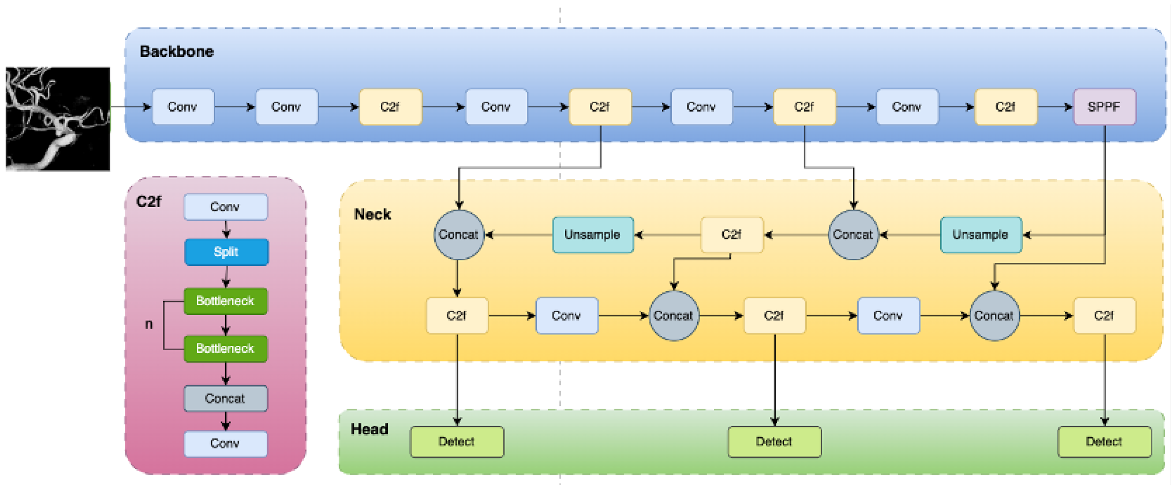
Figure 2.
AS-YOLO Network Architecture.
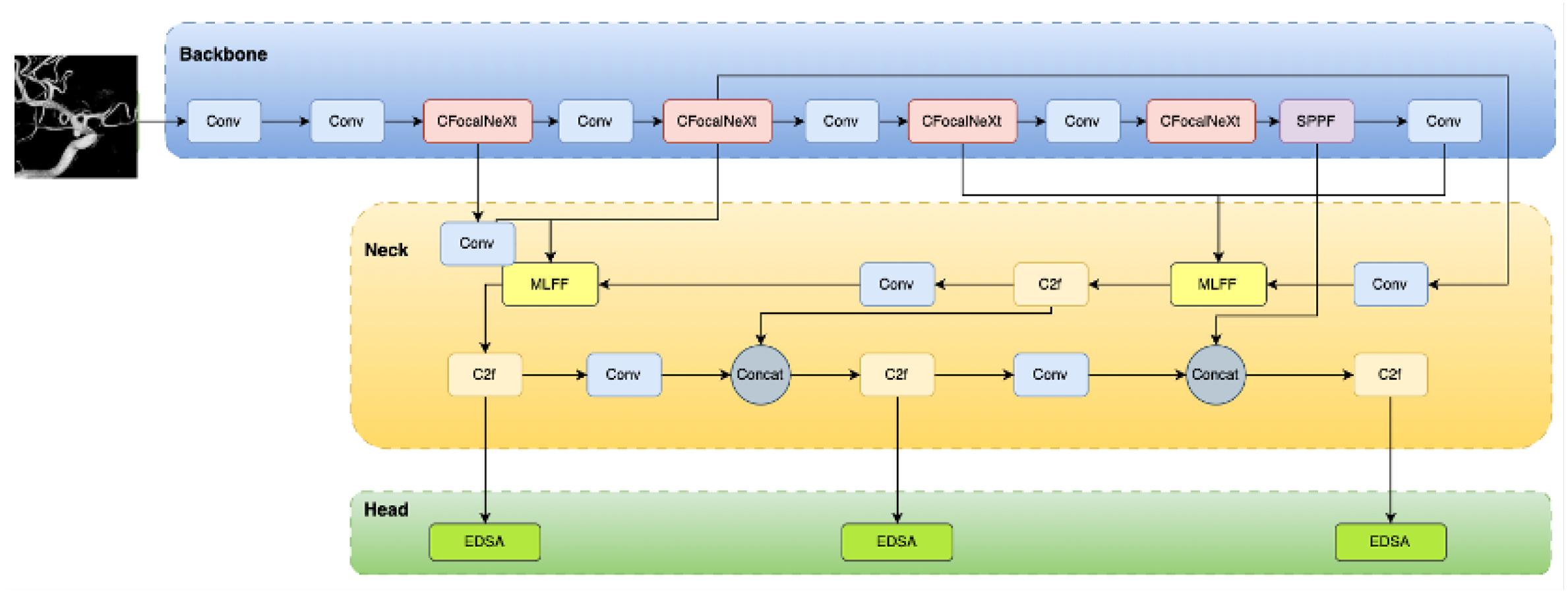
Figure 3.
CFNeXt Network Architecture.
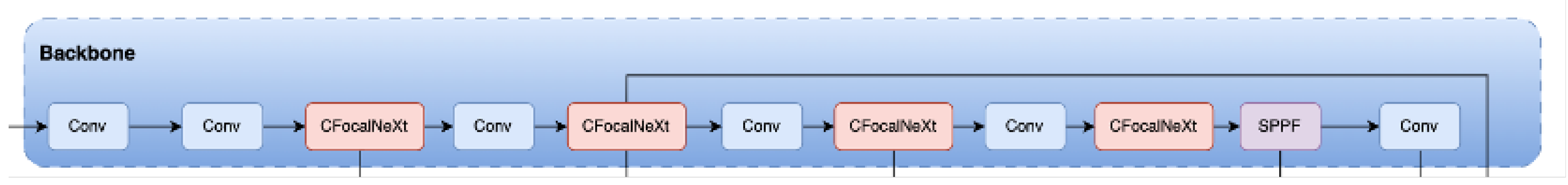
Figure 4.
On the left is the CFocalNeXt network architecture, and on the right is the FocalNeXt architecture.
Figure 4.
On the left is the CFocalNeXt network architecture, and on the right is the FocalNeXt architecture.
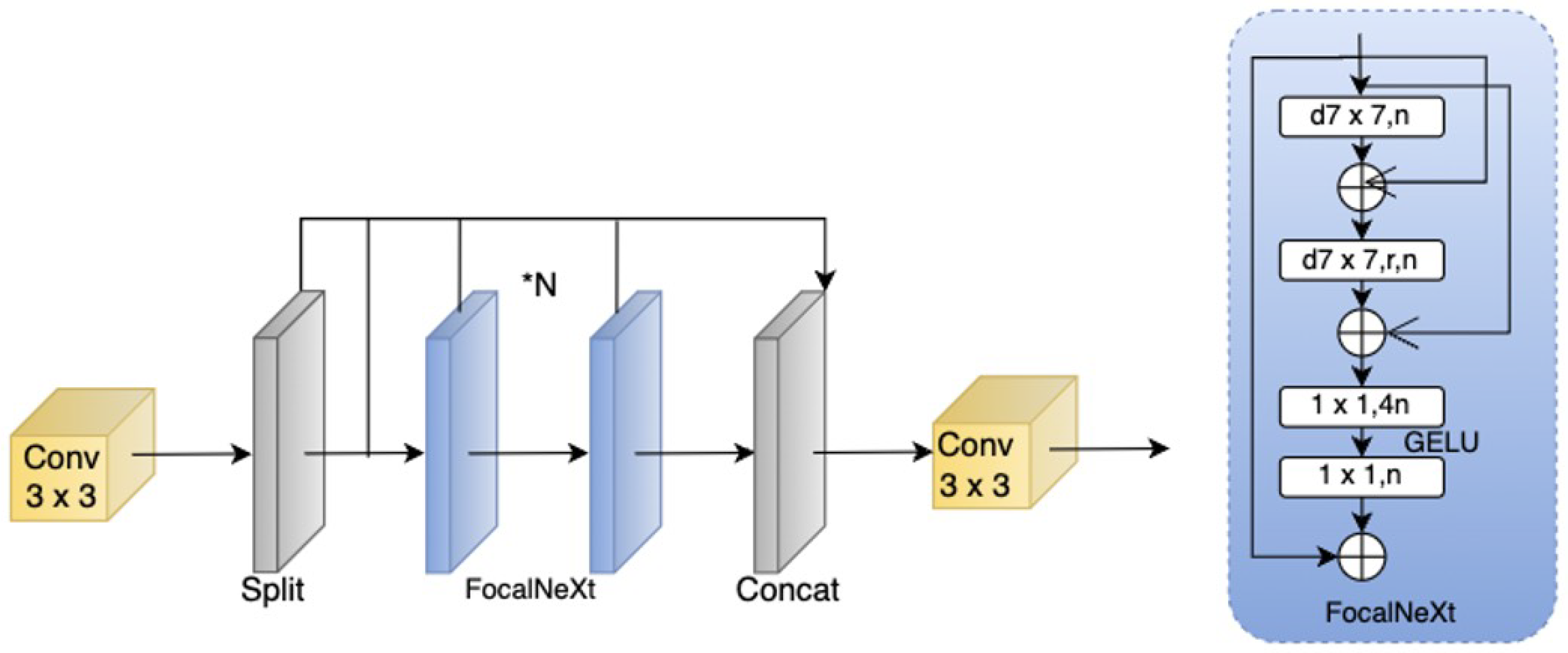
Figure 6.
MLFF and MFFPN Network Architecture. (a) MLFF architecture. (b) MFFPN architecture.
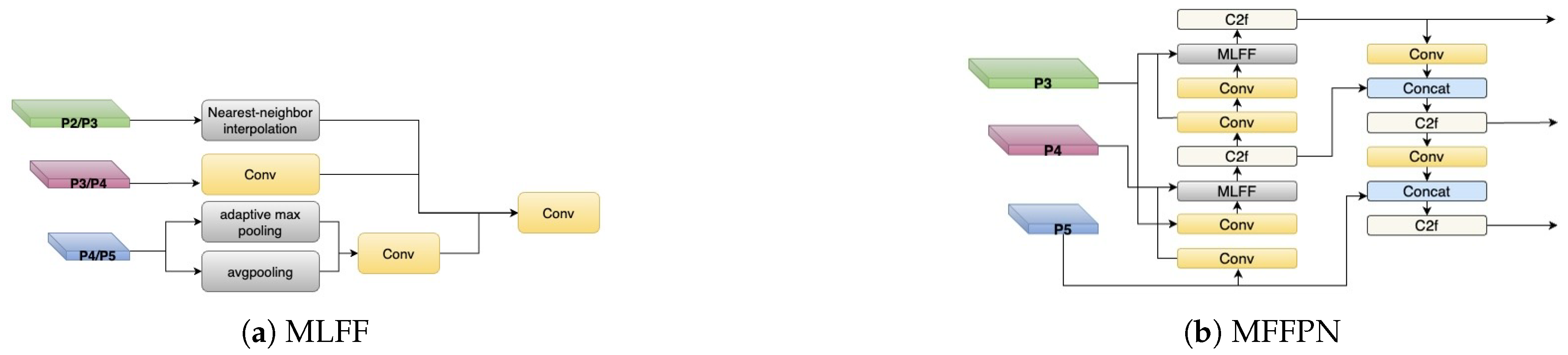
Figure 7.
Comparison of YOLOv8 and EDSA Detection Head Structures. (a) YOLOv8 Detection Head Architecture. (b) Efficient Depthwise Separable Convolutional Aggregation Detection Head Architecture.
Figure 7.
Comparison of YOLOv8 and EDSA Detection Head Structures. (a) YOLOv8 Detection Head Architecture. (b) Efficient Depthwise Separable Convolutional Aggregation Detection Head Architecture.
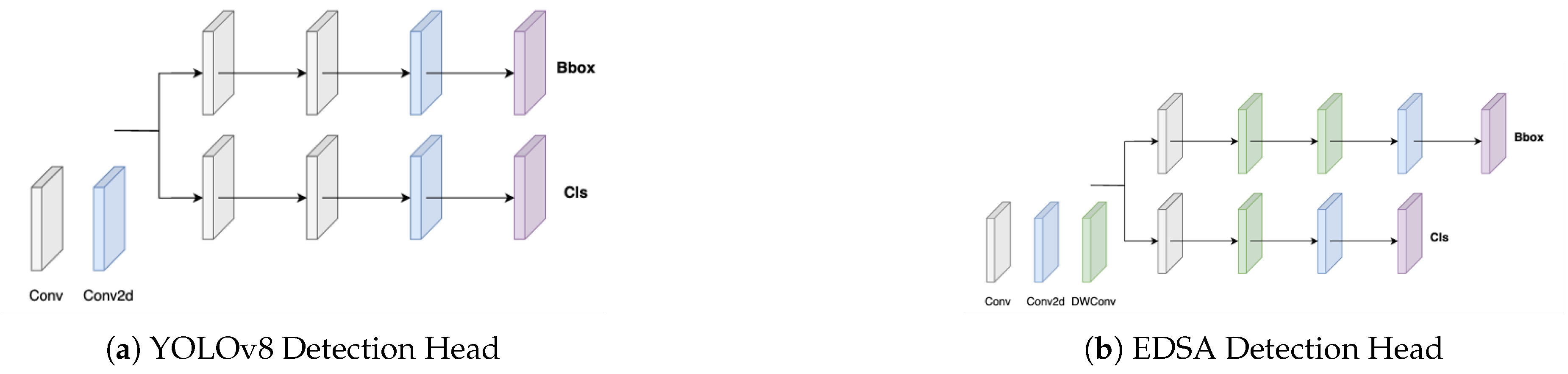
Figure 8.
PR curve comparison between YOLOv8 and AS-YOLO. (a) YOLOv8 PR Curve. (b) AS-YOLO PR Curve.
Figure 8.
PR curve comparison between YOLOv8 and AS-YOLO. (a) YOLOv8 PR Curve. (b) AS-YOLO PR Curve.
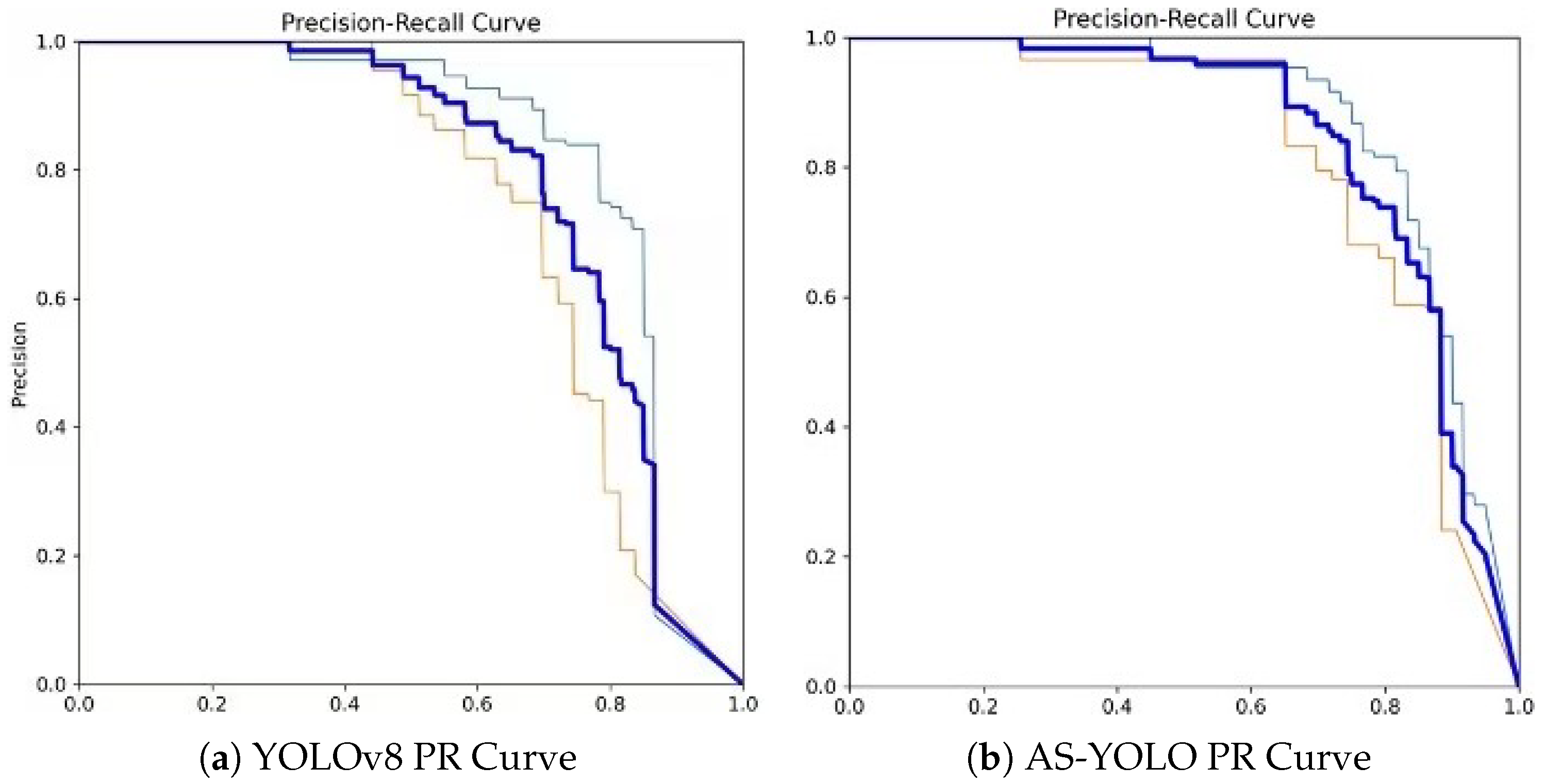
Figure 9.
Heatmap comparison between YOLOv8 and AS-YOLO. (a) and (c) are the heatmaps of the same image generated by YOLOv8 and AS-YOLO, respectively. (b) and (d) are the heatmaps of another image generated by YOLOv8 and AS-YOLO, respectively.(a) YOLOv8 Heatmap 1. (b)YOLOv8 Heatmap 2. (c) AS-YOLO Heatmap 1. (d) AS-YOLO Heatmap 2.
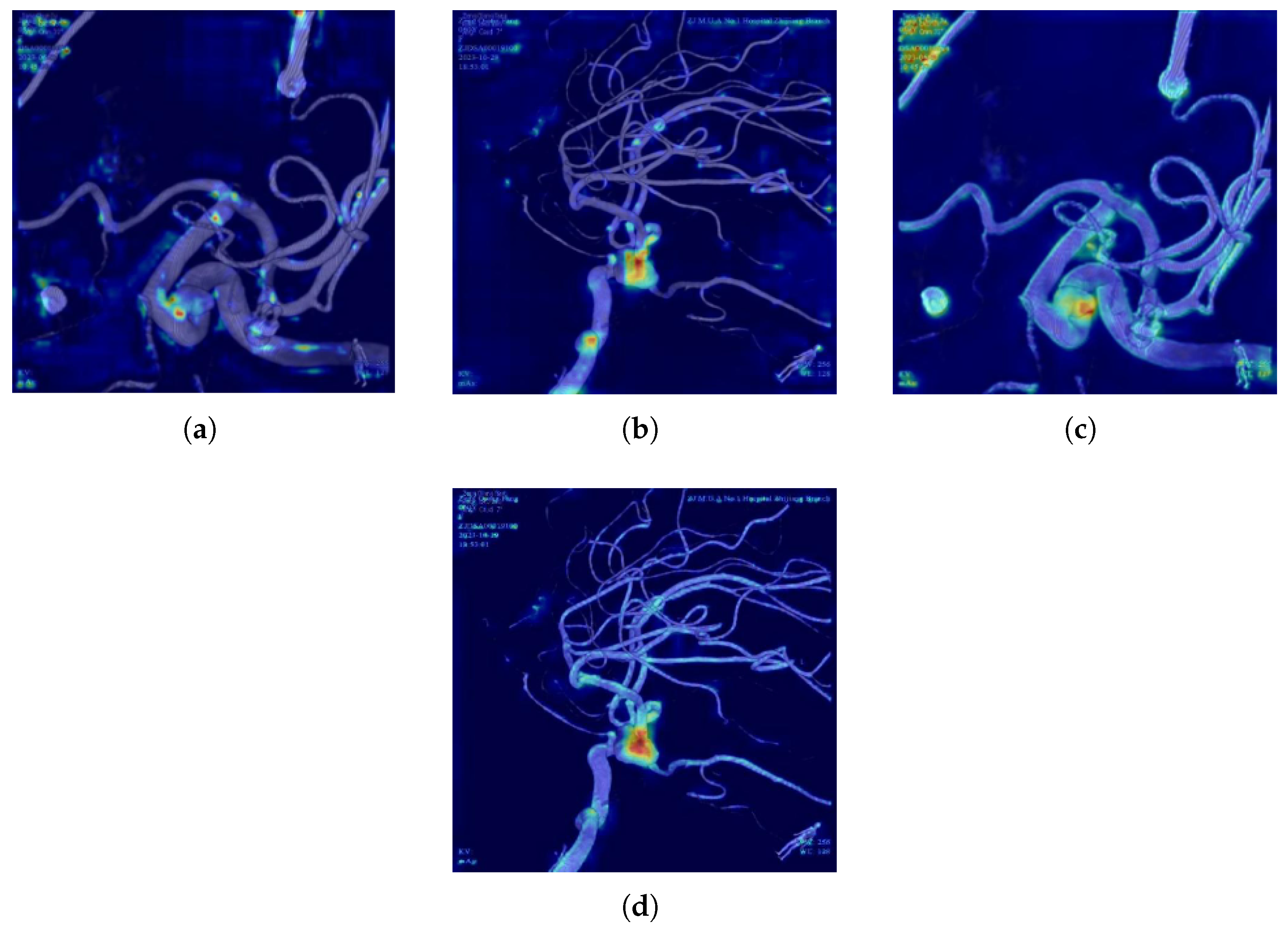
Figure 10.
Performance comparison chart of each model.
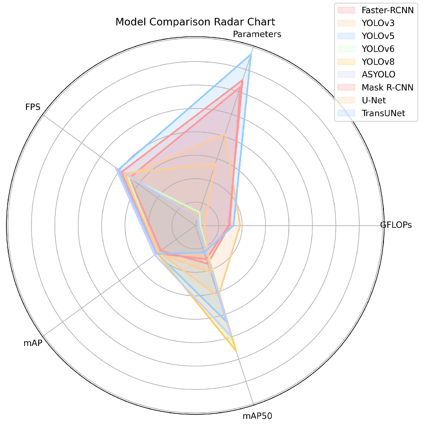
Figure 11.
Detection results of various algorithms on sidewall-type aneurysm images. Each subfigure illustrates the detection performance of the algorithm on aneurysm images. From the figure, it can be concluded that AS-YOLO achieves the best detection performance.(a) Original Image. (b) The detection results of Faster R-CNN. (c)The detection results of YOLOv6. (d) The detection results of YOLOv8. (e) The detection results of TransUNet. (f) The detection results of AS-YOLO.
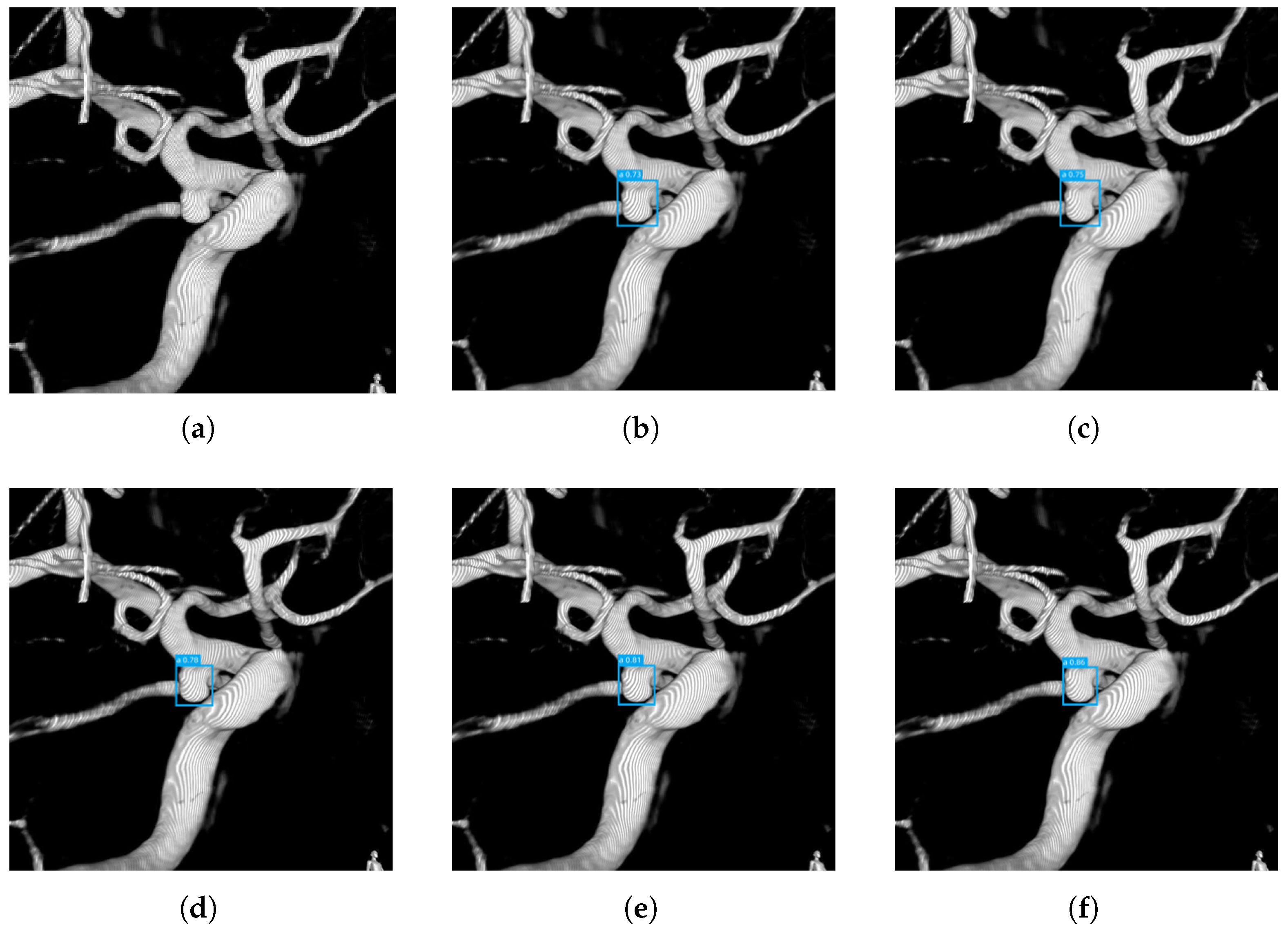
Table 7.
Experiment result of ablation experiment.
| Method | Sidewall type | Bifurcation type | Params(M) | GFLOPs | |||||
|---|---|---|---|---|---|---|---|---|---|
| CFNeXt | MLFF | EDSA | SIoU | mAP0.5 | mAP0.5:0.95 | mAP0.5 | mAP0.5:0.95 | ||
| 0.815 | 0.444 | 0.735 | 0.362 | 3.006 | 8.1 | ||||
| ✓ | 0.860 | 0.452 | 0.750 | 0.375 | 2.662 | 7.2 | |||
| ✓ | 0.835 | 0.455 | 0.741 | 0.373 | 3.057 | 8.3 | |||
| ✓ | 0.813 | 0.440 | 0.727 | 0.355 | 2.707 | 6.9 | |||
| ✓ | 0.825 | 0.452 | 0.741 | 0.369 | 3.006 | 8.1 | |||
| ✓ | ✓ | 0.865 | 0.465 | 0.755 | 0.377 | 2.714 | 7.4 | ||
| ✓ | ✓ | 0.820 | 0.450 | 0.738 | 0.366 | 2.706 | 6.8 | ||
| ✓ | ✓ | ✓ | 0.864 | 0.463 | 0.748 | 0.372 | 3.050 | 7.7 | |
| ✓ | ✓ | ✓ | ✓ | 0.868 | 0.468 | 0.760 | 0.379 | 2.759 | 7.1 |
* ✓ indicates the module used.
Table 8.
Experiment results of contrast experiment.
| Type | Result | Faster R-CNN | YOLOv3 | YOLOv5 | YOLOv6 | YOLOv8 | Mask R-CNN | U-Net | TransUNet | AS-YOLO |
|---|---|---|---|---|---|---|---|---|---|---|
| Bifurcation | mAP0.5 | 0.736 | 0.764 | 0.792 | 0.793 | 0.815 | 0.817 | 0.786 | 0.834 | 0.868 |
| mAP0.5:0.95 | 0.384 | 0.401 | 0.431 | 0.436 | 0.444 | 0.446 | 0.426 | 0.454 | 0.468 | |
| Sidewall | mAP0.5 | 0.654 | 0.682 | 0.724 | 0.725 | 0.735 | 0.739 | 0.724 | 0.79 | 0.760 |
| mAP0.5:0.95 | 0.344 | 0.356 | 0.369 | 0.361 | 0.362 | 0.366 | 0.364 | 0.368 | 0.379 |
Table 9.
Experiment results of contrast experiment.
| Method | Params(M) | GFLOPs | mAP0.5 | mAP0.5:0.95 | FPS |
|---|---|---|---|---|---|
| Faster R-CNN | 29.269 | 124.4 | 0.695 | 0.364 | 34.3 |
| YOLOv3 | 38.269 | 82.1 | 0.723 | 0.3875 | 63.5 |
| YOLOv5 | 2.503 | 7.1 | 0.758 | 0.405 | 86.3 |
| YOLOv6 | 4.234 | 11.8 | 0.710 | 0.404 | 104.2 |
| YOLOv8 | 3.006 | 8.1 | 0.775 | 0.403 | 112.6 |
| Mask R-CNN | 28.524 | 130.6 | 0.778 | 0.406 | 30.2 |
| U-Net | 7.838 | 55.3 | 0.755 | 0.395 | 42.0 |
| TransUNet | 32.623 | 153.7 | 0.812 | 0.411 | 24.3 |
| AS-YOLO | 2.759 | 7.1 | 0.843 | 0.428 | 99.6 |
Disclaimer/Publisher’s Note: The statements, opinions and data contained in all publications are solely those of the individual author(s) and contributor(s) and not of MDPI and/or the editor(s). MDPI and/or the editor(s) disclaim responsibility for any injury to people or property resulting from any ideas, methods, instructions or products referred to in the content. |
© 2025 by the authors. Licensee MDPI, Basel, Switzerland. This article is an open access article distributed under the terms and conditions of the Creative Commons Attribution (CC BY) license (http://creativecommons.org/licenses/by/4.0/).
Copyright: This open access article is published under a Creative Commons CC BY 4.0 license, which permit the free download, distribution, and reuse, provided that the author and preprint are cited in any reuse.


