

Submitted:
30 December 2025
Posted:
31 December 2025
Read the latest preprint version here
Abstract
On the basis of the isomorphic algebraic structures of the field of complex numbers ℂ and the 2-dimensional Euclidean field of real vectors V₂, in terms of identical geometric products of elements, this paper brings integral identities for scalar and vector fields in V₂, which are vector analogues of the well-known integral identities of complex analysis. Consequently, in this paper, Theorem 1., which is a generalized fundamental theorem of integral calculus in the field V₂, is the vector analogue of the Cauchy theorem of complex analysis. Therefore, special attention is paid to the vector analogue of Cauchy's calculus of residues in the field V₂. Finally, at the very end of the paper, the algebraic structure of the 3D field of vectors V₃ is presented, as well as the corresponding fundamental integral identities.
Keywords:
geometric product
; the field of vectors
MSC: Primary 14A05; 26B12; Secondary 14A25; 26B20
1. Introduction
A geometric algebra (Clifford algebra) is an extension of elementary algebra to work with geometrical objects such as vectors. It is built out of two fundamental operations: addition and geometric product, [2]. The multiplication of vectors alone results in objects called multivectors, among which are bivectors, the name applied in this paper to the objects of the bivector field , corresponding to the field of vectors . Compared with other formalisms for manipulating geometric objects, geometric algebra supports dividing by a vector. The geometric product was first mentioned by Grassmann, who founded the so-called external algebra, [3]. After that, Clifford himself greatly expanded upon Grassmann’s work, to form geometric algebra, named after him Clifford algebra [2], by unifying both Grassmann’s algebra and Hamilton’s quaternion algebra. In the middle of the 20th century, Hestenes repopularized the term geometric algebra [4,5].
On the other hand, although rarely used explicitly, a geometric representation of complex numbers is implicitly based on its structure of the Euclidean 2-dimensional vector space. If the binary operation of the product of two complex numbers and z is considered as the sum of the inner product and outer product , where and į, and i is an imaginary unit, it can be said that is in the form of a geometric product of two ivectors (two complex numbers), as two geometric objects belonging to the ivector field (to the field of complex numbers ). For any complex number z, its absolute value is its Euclidean norm denoted by r, and the argument is the polar angle . Since ordered pairs represent both complex numbers and vectors, the binary operation of the product of two complex numbers (two ordered pairs), in the form of the geometric product (), will be the basis for modifying Grassmann’s geometric product of vectors, which is defined as the sum of the inner (scalar) and outer (bivector) products of two vectors. By this modification, the geometric product of two vectors becomes commutative, similar to the product of complex numbers themselves, which still supports vector division. In this manner, a complete analogy is established between the algebra of complex numbers and the modified Clifford algebra in the Euclidean 2-dimensional field of vectors . On the basis of that analogy, Section 2 of the paper presents the most important vector integral identities, in the Euclidean field of real vectors , which are vector analogies to the well-known integral identities of complex analysis.
In the next section (Section 3), the algebraic structure of the field of vectors is defined. In addition, this section brings the corresponding integral identities, which are more general than the fundamental integral identities of the Stokes theorem and the divergence theorem.
1.1. Realireal Vector Space
The ordered pairs and į are the basis of the 2-dimensional realireal vector space [6], which is the Cartesian product of a 1-dimensional real vector space and a 1-dimensional ireal vector space , and as such is an additive Abelian (commutative) group of elements į. As both of these 1-dimensional vector spaces are defined over the field of real numbers , the real vector space can be said to be a field of real numbers , whereas the ireal vector space cannot be a field, and therefore not a field of imaginary numbers . On the other hand, if the vector space is complemented by a binary operation of the product of two elements and , which corresponds to the matrix product, in such a manner that
where both the commutative axiom of multiplication and the associative axiom of multiplication are satisfied, as well as the distributive axiom, and in addition the element , which corresponds to the inverse matrix , is the inverse element of the element , then the 2-dimensional realireal vector space can be said to be defined over the field of complex numbers , that is, is the field of complex numbers . More precisely, on the one hand, the ordered pair is the vector space over the scalar field of real numbers , and on the other hand, after complementation with the binary operation of the product of the elements, the ordered pair is the vector space over the ivector field , that is, is the ivector field . Accordingly, complex numbers z can be said to be ivectors į, the elements of the vector space , that is, of the ivector field and as such can be multiplied either by real numbers as scalars or by complex numbers as ivectors. When the ivector is multiplying by the imaginary unit i, then the order of the elements, in the resulting ordered pair, is changed, so the resulting ordered pair is not an element of the ivector field . Therefore, from that perspective, multiplying complex numbers by imaginary numbers is absolutely unacceptable. A complex number z can be multiplied by the ivector į, so that į=įį and į2 = įį .
How the operator cįs·= has the most important properties of an exponential function, since cįs·cįs·= cįs, (cįscįs and d(cįs=įcįs·d·, the operator į can be said to be the exponential form of the operator cįs·. For above reason, multiplication of the operator cįs·= by imaginary numbers is unacceptable, but multiplication by either a real number or an ivector is acceptable.
1.2. Algebraic Structure of the Field of Real Vectors
The basis of the 2-dimensional real vector space (the Cartesian square of the 1-dimensional real vector space ), as an additive Abelian group of elements , consists of ordered pairs and , such that . Analogous to the binary operation of the product of the elements, which we used to complement the realireal vector space , it is also possible to complement the vector space , with the binary operation of the product of two elements and , which corresponds to the matrix product, in such a manner that
where the element , which corresponds to the inverse matrix , is the inverse element of the vector space . In this case both the commutative axiom of multiplication and the associative axiom of multiplication are satisfied, as well as the distributive axiom. Therefore, on the one hand, the ordered pair is the vector space over the scalar field of real numbers , whereas on the other hand, the ordered pair is a vector space over the bivector field , that is, is the bivector field , whose elements are the bivectors . Accordingly, the bireal numbers w are bivectors , elements of the vector space , that is, of the bivector field and as such can be multiplied either by real numbers as scalars or by bireal numbers as bivectors.
The field of real vectors, denoted by , corresponds to the bivector field , in the sense of the correspondence: and , where the unit vectors and are orthogonal basis vectors of the field . The vectors , as elements of the field , correspond to the bireal numbers . In other words, there is a one to one correspondence between the fields and . If , then is a norm over both fields and , simultaneously, and . Consequently, . It is quite clear that the inverse element allows division by a vector in the field . The binary operation of the product of two vectors, belonging to the field , defined as follows.
Definition 1.
Let and be two vectors in . Then, the commutative binary operation
is the geometric product of and .
Obviously, . Here, and , where is the angle between and .
The geometric product of and corresponds to the product of two bivectors and , so that
In addition, and
The concepts of geometric product and bivector, introduced above, are closely related to the same concepts in Clifford algebra [2]. However, there is evidently a crucial difference between Clifford algebra and the algebra of the field , which is reflected in the fact that the geometric product of the elements of the field , on the one hand, is the element of the field , corresponding to the bivector, the element of the bivector field , and on the other hand, it is also commutative, which means that the field , in addition to being an additive Abelian group, is also a multiplicative Abelian group.
If is the unit vector of the vector , then and
so that
where i are the symmetric and antisymmetric parts of the geometric product , respectively. Therefore, to emphasize once again, the geometric product of two vectors is a vector in . Accordingly, and . The vector is orthogonal to the vector , that is, is the vector obtained by rotating the vector , where is the angle between the vector and the vector , by radians in the positive mathematical direction. In addition, the unit vector is the inverse vector of the unit vector of the vector , and therefore also the unit vector of the inverse vector of the vector , so that and .
The main purpose of the next section is to derive vector integral identities, in the field of vectors , which are analogous to the known integral identities of complex analysis, on the basis of the analogy of the ivector field and the bivector field , which corresponds to the field of vectors .
2. Differential and Integral Calculus in
As cs·cs·=cs, (cscs i d(cscs·d·, the bivector operator cs· also has the properties of an exponential function, similar to the ivector operator cįs·. The operator is the exponential form of the operator cs·. Since =cs, one more analogy with complex analysis is the notion of the so-called vector logarithmic function , where . In addition, Log, . Let sc. The ordered pair of vectors is the inverse orthonormal basis with respect to the orthonormal basis of the field . For an arbitrary vector , the vector is the rotated vector , in the positive mathematical direction, by the angle , and the vector by the angle . The geometric products of the vector with the inverse basis vectors and rotate the vector by the angles and , respectively, in the positive mathematical direction.
On the basis of the geometric products , and , as well as,
and (), all other combinations of geometric products of the basis vectors , , and can also be obtained.
If we introduce the differential operator , then . Hence, and . Since and , the vector operators of partial derivatives are introduced, as a vector analogue of the Virtinger operators [16],
Here,
It is important to emphasize that when geometric products and geometric quotients are differentiated, the same rules apply as when ordinary products and quotients are differentiated, so that . Let’s prove this,
Definition 2.
The geometric product is an operator of a differential form.
The vector operator
is a radial vector differential operator. The vector operator
is a transverse vector differential operator.
It is obvious that is a gradient operator. The symmetric part of the geometric product is the divergence vector (div) of the vector field , and the antisymmetric part is the curl of , since
On the other hand,
Consequently,
so that and . Similarly,
Further, since cs, it follows that ,
Therefore,
In addition,
In accordance with above,
since . The vector identity just derived can be obtained explicitly, if we introduce the determinant of the Jacobi matrix (Jacobian) of the bijective mapping , defined by the system of vector equations and , as follows
In this case, , which leads to (2.14). The vector , corresponding to the bivector of the bivector field , is the Lebesgue measure of the infinitesimal surface of the field of vectors .
Definition 3.
Let . Then, the geometric product is an operator of a differential form.
2.1. Generalization of the Fundamental Theorem of Integral Calculus in
Let be a closed smooth Jordan curve, which is the boundary of an arbitrary region G in , and () be isolated points on the curve , surrounded by circles with centers at and arbitrarily small radius , which intersect the curve at points and and do not intersect each other. If () are isolated points in G , surrounded by circles , which do not intersect each other, then it is possible to form a simply connected region , inside which all points and are, by connecting the circles , successively, the first with the second, the second with the third, etc., using parallel straight line segments and , at a mutual distance , as well as by connecting the circles on the curve with the circles , one-to-one, using the parallel straight line segments and , at a mutual distance . The boundary of (blue region in Figure 1), inside G, divides the region G into subregions .
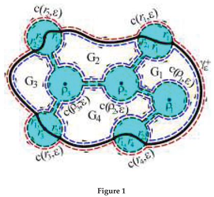
Accordingly, the vector integral operator over is introduced, as follows
where denotes the total value of an improper integral [9,10,11,12,13,14], such that
and denotes the Cauchy principal value. The vector integral operator
where , that is, , as well as and , is the residue operator in G.
The vector integral operator over G is introduced, as follows
Here, , and
so that
since
Obviously,
Definition 4.
Let denote the vector differential form obtained by applying to some scalar or vector field in , which has continuous partial derivatives at every point of G. Then, is regular in G.
Definition 5.
Let be regular almost everywhere in G(everywhere except on the finite set of singular points and . Then, is integrally summable on the set S if and only if
The proof of the fundamental theorem that follows, as can be seen, is an explicit consequence of Green’s theorem [6].
Theorem 1.
Let and be regular almost everywhere in G(everywhere except on the finite set of singular points and . Then,
where .
Proof.
□
Remark 1.
If the set of singular points, either on the contour γ or in the region G, is an empty set, then the choice of a representative point (either on the contour γ or ϱ in the region G, respectively) is arbitrary. If, in addition, the field is uniform [7], then , so in that case, the choice of representative points is not necessary. On the contrary, if there is a limit , and tends to infinity as ε tends to zero, then the limit is also infinite. Obviously, the indeterminate form of the difference of two infinities, in this emphasized case, leads to the finite limit .
If , then and
since
Clearly, .
2.2. Integrals of Scalar and Vector Fields
The vector differential of a scalar field is as follows
where . The second vector partial derivative of F is the first vector partial derivative of the vector field , so that
If and are uniform vector fields, then by applying the vector integral operator (2.30) to the scalar field F, a vector integral identity is obtained
where . An integral identity of complex analysis, which is an analogue of the vector integral identity (2.36), is the integral identity of Cauchy’s integral theorem [7].
As and if, in addition, , then , that is,
A vector field , satisfying theCauchy-Riemann condition , is said, analogous to complex analytic functions, to be an analytic vector field. Hence, an analytic vector field is a vector derivative of the Laplace scalar field F. Clearly, the coordinate components of the analytic vector field are also Laplace scalar fields.
Assume that the analytic vector field , as the vector derivative of the Laplace scalar field F, is not defined at the point , where G is a region in the field of vectors , bounded by a closed smooth Jordan curve , as well as at point on curve . The vector integral identity
is a vector analogue of the integral identity of Cauchy’s integral theorem, which is slightly generalized, since in this emphasized case
Definition 6.
If a vector field is differentiable (regular), but not analytic, in an arbitrary region G of the field , bounded by a closed smooth Jordan curve γ, then the gradient of , as the surface (spatial) derivative of , is defind by
where .
Remark 2.
Obviously, some vector field is regular if and only if the differential form is regular. The gradient defined above is the vector analogue in of the Pompeiu areolar derivative of a complex function, [8].
Similarly, based on the vector identity (2.9), the so-called cumulative surface (spatial) derivative of can be defined as follows.
Definition 7.
If a vector field is differentiable (regular), but not analytic, in an arbitrary region G of the field , bounded by a closed smooth Jordan curve γ, then the cumulative surface (spatial) derivative of is defind by
By (2.41), if is a regular and uniform vector field in the -neighborhood of its singular point and , then
If , then , which is another vector analogy to the well-known result of complex analysis. Let be an analytic vector field, such that leads to the determinate form only after the application of L’Hospital’s rule n times. Then, the vector formula for , being analogous to the complex analysis formula, can be obtained via the vector identity , see (2.38), where . Namely, since the same vector identity applies to the analytic vector field , it follows that
Accordingly, applying L’Hospital’s rule,
Further, since is an analytic vector field, it follows that
This means that L’Hospital’s rule can be explicitly applied to the vector field .
If some analytic vector field is regular in an arbitrary region G bounded by a closed smooth Jordan curve , then for the vector field
where , according to (2.39), (2.46) and (2.48), the following is true
Hence
since , whenever . This is the vector analogue of the well-known Cauchy’s integral formula.
If some vector field is such that the scalar fields F and have continuous first partial derivatives in region G, bounded by the closed smooth Jordan curve , almost everywhere (everywhere except on the singular set ), then by applying the vector integral operator (2.30) to the vector field , one comes to the following vector integral identity
since
Consequently,
Clearly, in the general case, is not the same as . Namely,
So, differs from . Accordingly,
since
which can be explicitly obtained if in (2.9) is formally replaced by . Therefore, the two identities 5. and 6., on page 85., in Section 3.16., Chapter 3., in [15], should be replaced by: 5. and 6. if is either an analytic vector field () or a Laplace vector field (). In both of these cases, the vector field satisfies Laplace’s equation .
Consequently,
On the other hand, let be continuous in an arbitrary region G bounded by a closed smooth Jordan curve , in which the partial derivatives , , and exist and satisfy the Cauchy-Riemann equations
Then, according to the Looman-Menchoff theorem [1], both the analytic vector field and the Laplace vector field can be said to be regular (holomorphic) vector fields in G. Therefore, on the basis of (2.50),
In addition,
where and . These vector integral formulas are analogous to the Cauchy-Pompeiu integral formula of complex analysis [17].
On the basis of the previous results one can say that there is a complete analogy between complex analysis in and real vector analysis in , thus all the results of complex analysis are applicable to scalar and vector fields in and vice versa. In doing so, z is formally replaced by , and the imaginary unit i, more precisely the ivector į, is replaced by the vector and vice versa ( and į). This conclusion can be even more obvious if a formally analogous method of deriving previously obtained vector identities is applied to the field of complex vectors , which corresponds to the ivector field (field of complex numbers) , in the sense of the correspondence: and į≒ , where the unit vector and the pseudo-unit vector ) form an orthogonal basis of the field of complex vectors , whose algebraic structure is based on the geometric product of two complex vectors as follows [9]
3. Algebraic Structure of the Field of Vectors
The Euclidean space consists of three Euclidean spaces , which means that the field of vectors , isomorphic to it, consists of three fields of vectors , with base vectors and , such that and . Hence, the three plane vectors , where and , are component vectors of an arbitrary spatial vector , such that . An index repeated as subscript and superscript in a product represents summation over the range of the index, by the Einstein summation convention.
Definition 8.
Let and be component vectors of two vectors and in , respectively, such that . The commutative geometric product in is defined as the sum of the geometric products of the component vectors and , as follows
Since
it follows that and .
On the other hand, the vector
where and , such that
is the inverse vector of the spatial vector , which allows division by the vector in . If is denoted by the bracket , then
3.1. Integral Identities in
Let be a spatial vector field, such that
For the 1 vector differential forms in
where , the 2 vector differential forms in are as follows
where .
According to Theorem 1.,
where the regions , bounded by closed smooth Jordan curves , are the normal projections of the smooth surface in onto , so that
Furthermore, since, see (2.9),
the previous two vector identities leads to the generalized Stokes integral identity
where and , as well as to the vector integral identity
where . Obviously, the fundamental theorem in is as follows
Theorem 2.
Let and be regular almost everywhere in (everywhere except on the finite set of singular points). Then,
On the other hand, for an arbitrary region V in the field , bounded by a closed smooth surface , if an arbitrary vector field satisfies the conditions of the divergence (Gauss-Ostrogradsky) theorem, then a procedure, similar to that for obtaining the integral identity (2.27), leads to the following integral identities
where and . Therefore, since it follows that
In addition, if and , then
which is a generalization of the well-known integral formulas in field theory. In this acute case, is the vector differential form , such that
Consequently, another fundamental theorem in can be formulated as follows
Theorem 3.
Let and be regular almost everywhere in (everywhere except on the finite set of singular points). Then,
4. Conclusion
Based on the integral identities obtained in the previous sections, all fundamental integral identities, from Cauchy’s integral identity of complex analysis, through the Kelvin-Stokes(Green’s) integral identity and the Stokes integral identity, as well as Gauss-Ostrogradsky’s integral identity, all the way to the Newton-Leibniz formula [13], can be expressed by one vector integral identity
where is the boundary of the corresponding compact region in . For the Newton-Leibniz formula, the vector differential form is the vector field , such that
is an interval vector field and , where I is some compact interval of the real line and is the vector Lebesgue measure of I.
So, in (4.1)
Data Availability Statement
No datasets were generated or analysed during the current study.
Conflicts of Interest
The author declares that no funds, grants, or other support were received during the preparation of this manuscript. The author has no relevant financial or non-financial interests to disclose.
References
- Arsova, M. The Looman-Menchoff theorem and some subharmonic function analogues. Proc. Amer. Math. Soc. 1955, 6, 94–105. [Google Scholar] [CrossRef]
- Clifford, W. Applications of Grassmann’s Extensive Algebra. Amer. J. Math. 1878, 1(4), 350–358. [Google Scholar] [CrossRef]
- Grassmann, H. Die lineale Ausdehnungslehre ein neuer Zweig der Mathematik: dargestellt und durch Anwendungen auf die übrigen Zweige der Mathematik, wie auch auf die Statik, Mechanik, die Lehre vom Magnetismus und die Krystallonomie erläutert; O. Wigand: Leipzig, 1844. [Google Scholar]
- Hestenes, D. Multivector Calculus. J. Math. Anal. Appl. 1968, 24, 313–325. [Google Scholar] [CrossRef]
- Hestenes, D. Multivector Functions. J. Math. Anal. Appl. 1968, 24, 467–473. [Google Scholar] [CrossRef]
- Marsden, E. J.; Tromba, J. A. Vector Calculus, 6th Edition; W. H. Freeman and Company: New York, 2012. [Google Scholar]
- Mitrinović, S. D.; Kečkić, D. J. The Cauchy Method of Residues: Theory and Applications; D. Reidel Publishing Company, 1984. [Google Scholar]
- Pompeiu, D. Sur une classe de fonctions d’une variable complexe. Rendiconti del Circolo Matematico di Palermo 1912, 33(1), 108–113. [Google Scholar] [CrossRef]
- Sarić, B. The Fourier series of one class of functions with discontinuities. Dissertation, University of Novi Sad, Faculty of Science, Department of Mathematics and Informatics, 20 October 2009. [Google Scholar]
- Sarić, B. Cauchy’s residue theorem for a class of real valued functions. Czech. Math. J. 2010, 60(4), 1043–1048. [Google Scholar] [CrossRef]
- Sarić, B. On totalization of the H1-integral. Taiw. J. Math. 2011, 15(4), 1691–1700. [Google Scholar]
- Sarić, B. On totalization of the Henstock-Kurzweil integral in the multidimensional space. Czech. Math. J. 2011, 61(4), 1017–1022. [Google Scholar] [CrossRef]
- Sarić, B. On an integral as an interval function. Sci. Bull., Series A 2016, 78(4), 53–56. [Google Scholar]
- Sarić, B. On the HN-integration of spatial (integral) derivatives of multivector fields with singularities in RN. Filomat 2017, 31(8), 2433–2439. [Google Scholar] [CrossRef]
- Spiegel, R. M.; Lipschutz, S.; Schiller, J. J.; Spellman, D. Schaum’s outline of theory and problems of complex variables: with an introduction to conformal mapping and its application, 2nd ed.; McGraw-Hill Book Company: London, 1974. [Google Scholar]
- Tung, C. C. On Wirtinger derivations, the adjoint of the operator ∂¯, and applications. Izv. Math. 2018, 82(6), 1239–1264. [Google Scholar]
- Tutschke, W. Interactions between partial differential equations and generalized analytic functions. Cubo A Math. J. 2004, 6(1), 281–292. [Google Scholar]
Disclaimer/Publisher’s Note: The statements, opinions and data contained in all publications are solely those of the individual author(s) and contributor(s) and not of MDPI and/or the editor(s). MDPI and/or the editor(s) disclaim responsibility for any injury to people or property resulting from any ideas, methods, instructions or products referred to in the content. |
© 2025 by the authors. Licensee MDPI, Basel, Switzerland. This article is an open access article distributed under the terms and conditions of the Creative Commons Attribution (CC BY) license (http://creativecommons.org/licenses/by/4.0/).
Copyright: This open access article is published under a Creative Commons CC BY 4.0 license, which permit the free download, distribution, and reuse, provided that the author and preprint are cited in any reuse.