Submitted:
14 February 2025
Posted:
17 February 2025
You are already at the latest version
Abstract
Pottery is one of the most common and abundant types of human remains found in archaeological contexts. The analysis of archaeological pottery involves the reconstruction of pottery vessels from their sherds, which represents a laborious and repetitive task. In this work, we investigate a deep learning-based approach for making that process more efficient, accurate and faster. In that regard, given a sherd’s digital point cloud in a standard, so-called canonical position, the proposed method predicts the geometric transformation which moves the sherd to its expected position relative to the respective vessel’s coordinate system. Among the main components of the proposed method, a pair of deep 1D-convolutional neural networks trained to predict the 3D Euclidean transformation parameters stands out. Herein, rotation and translation components are treated as independent problems, so, while the first network is dedicated to predict translation moments, the other infers the rotation parameters. In practical applications, once a vessel’s shape is identified, the networks can be trained for predicting the target transformation parameter values. Given the 3D model of a vessel, it is broken virtually countless times for the production of training data, which consist of a large set of virtual sherds. The herein proposed 1D-convolutional neural network architecture, so-called PotNet, was inspired by the PointNet architecture. While PointNet was motivated by 3D point clouds classification and segmentation applications, PotNet was designed to perform non-linear regressions. Experiments using three distinct real vessels were carried out, and the reported results suggest that the proposed method can be successfully used for aiding pottery reconstruction.
Keywords:
1. Introduction
2. Related Works
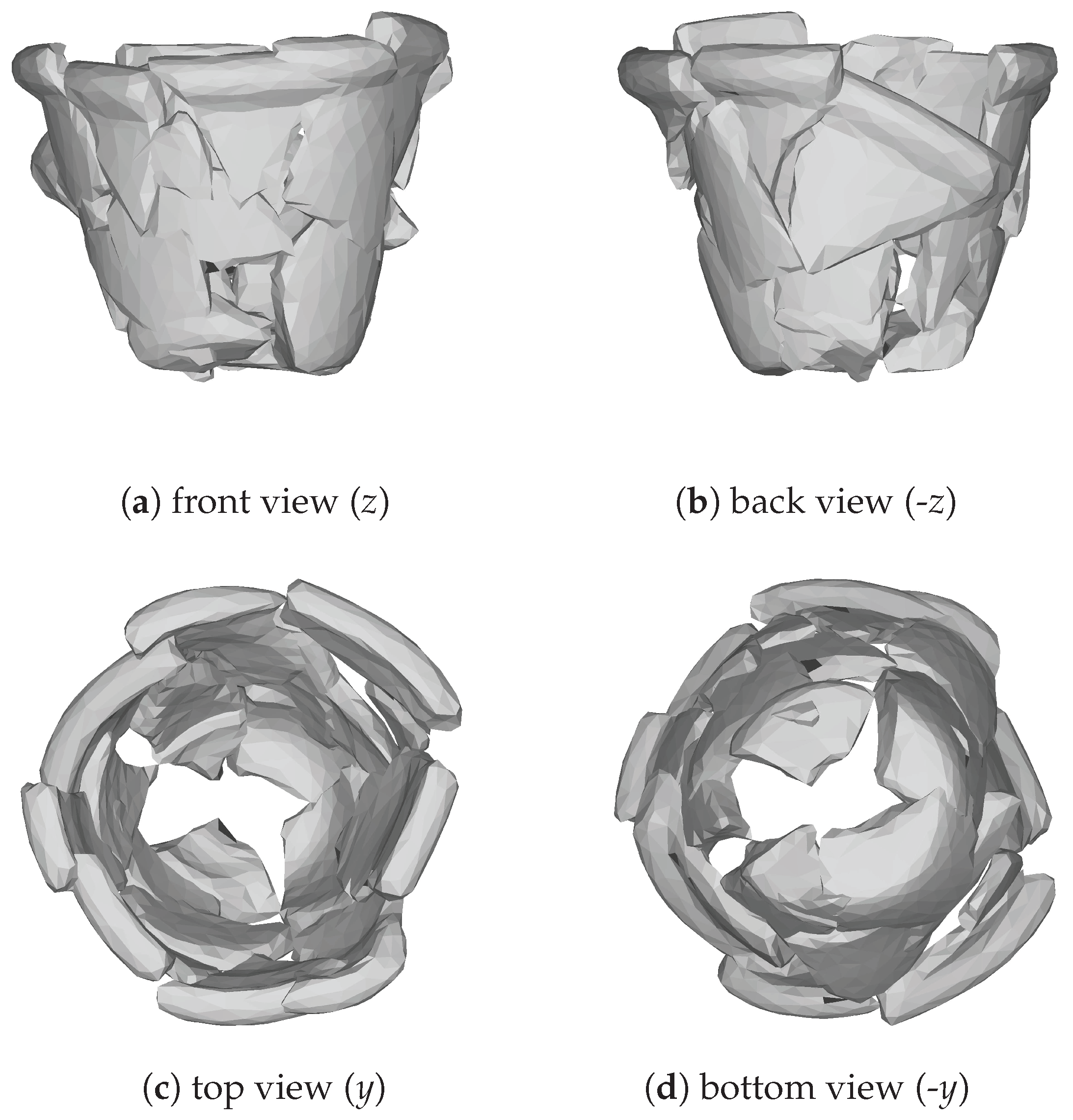
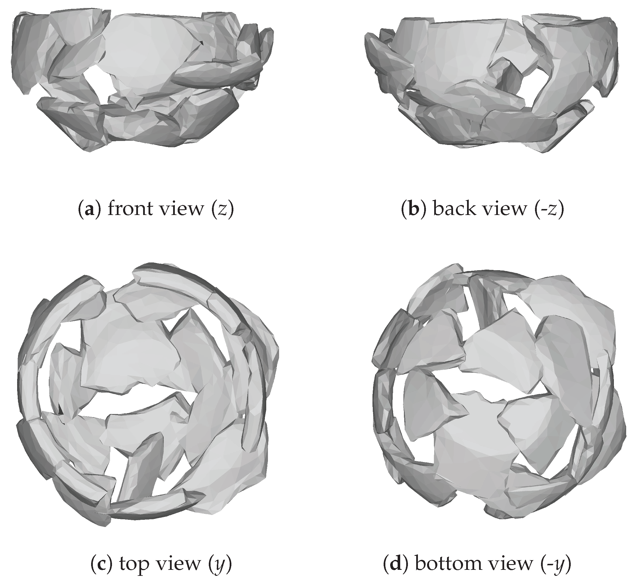
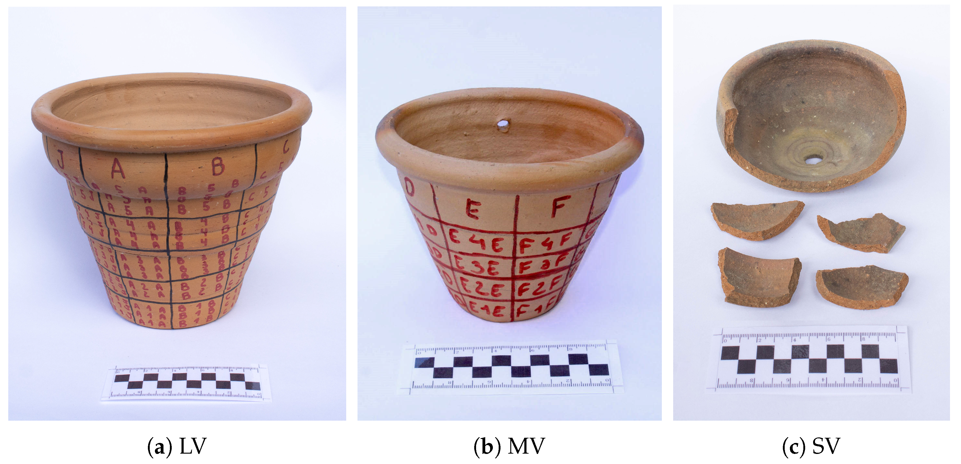
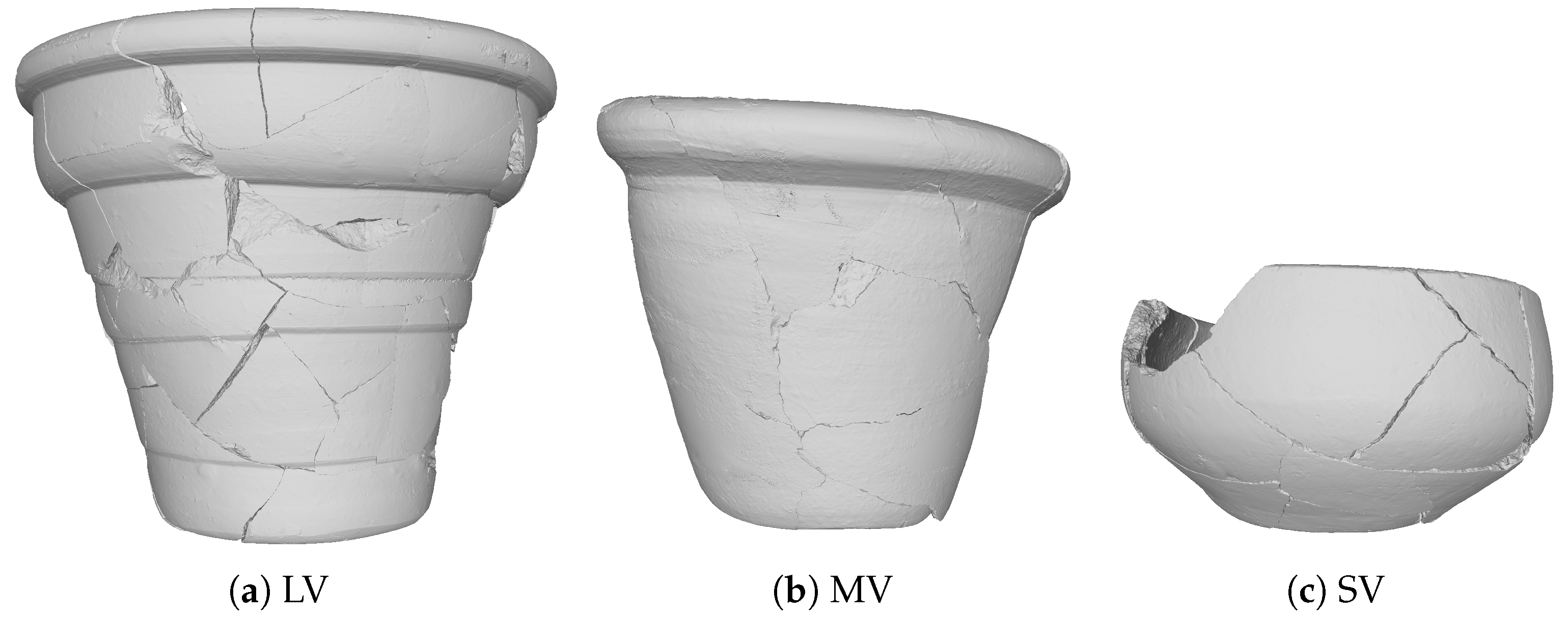
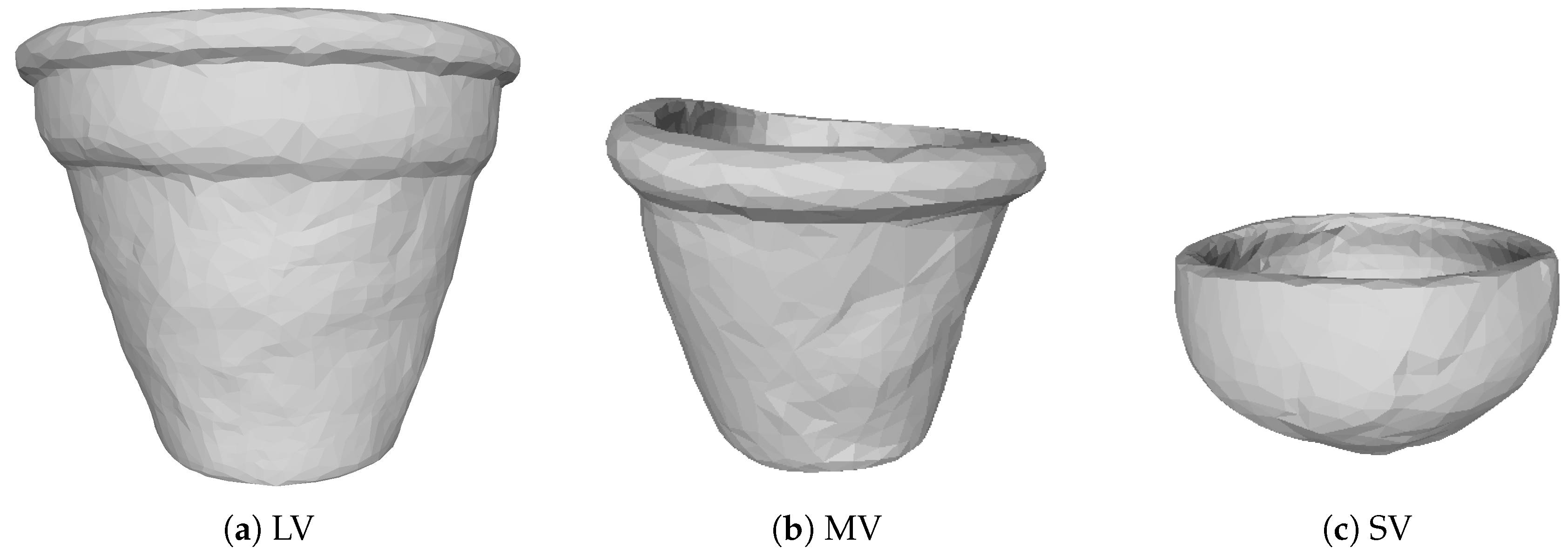
3. Materials
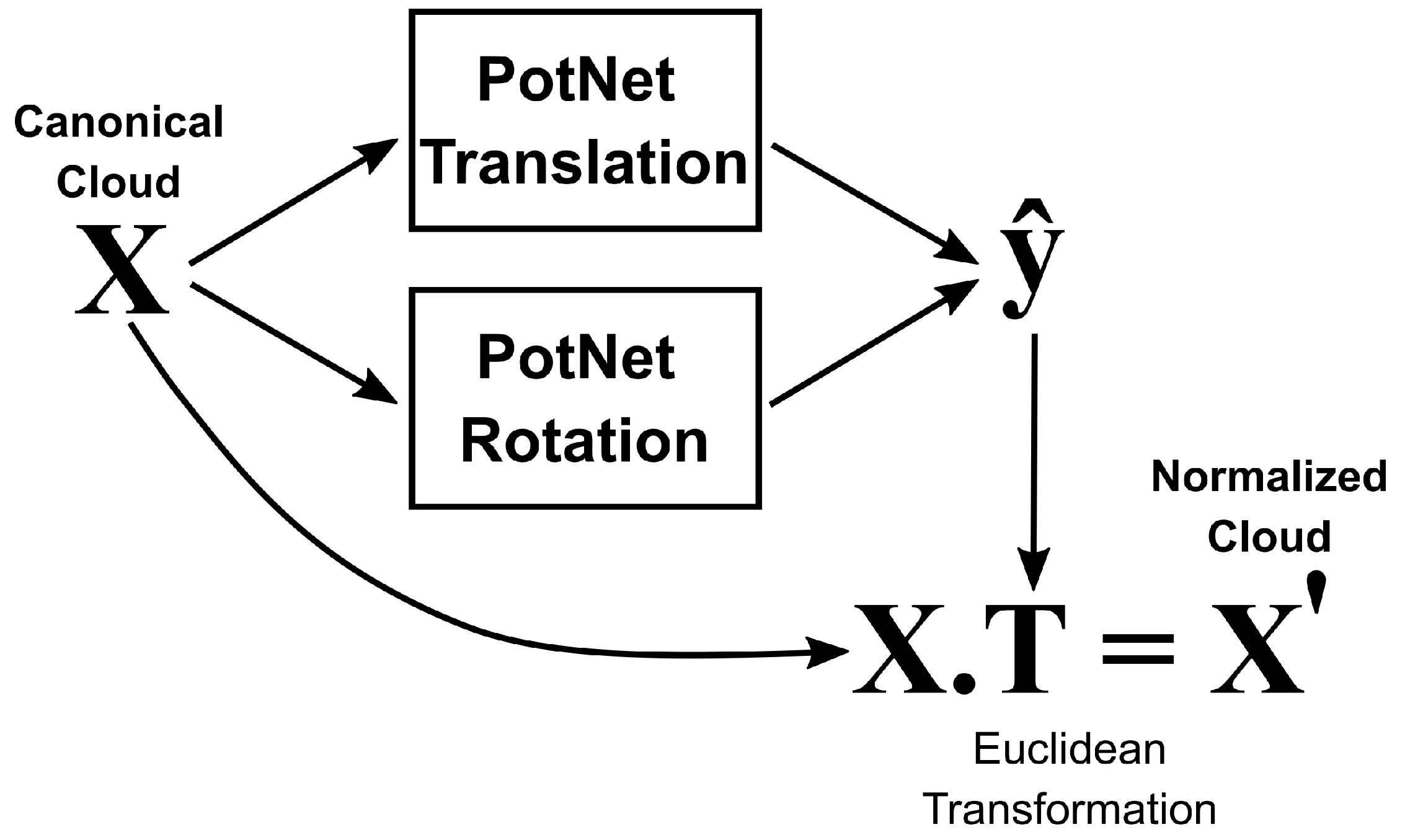
4. Proposed Method
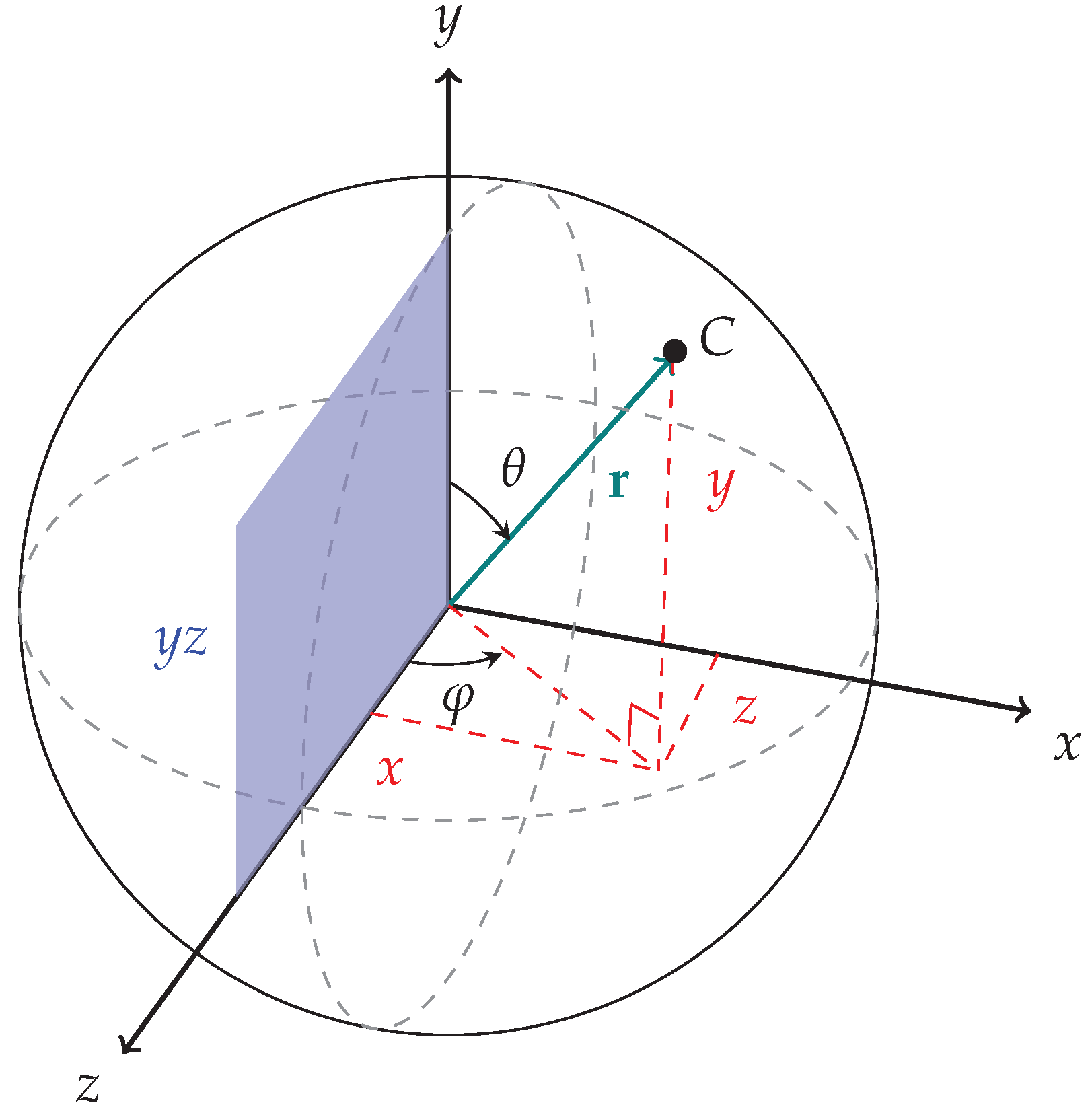
4.1. Problem Modeling
4.1.1. Normalized Cloud
4.1.2. Canonical Cloud
4.1.3. Target Euclidean Transformation
4.2. PotNet Model
4.3. Training Procedure
5. Experimental Setup
5.1. Virtual Shattering Procedure
5.2. Synthetic Sherds Datasets
5.3. Training
6. Results and Discussion
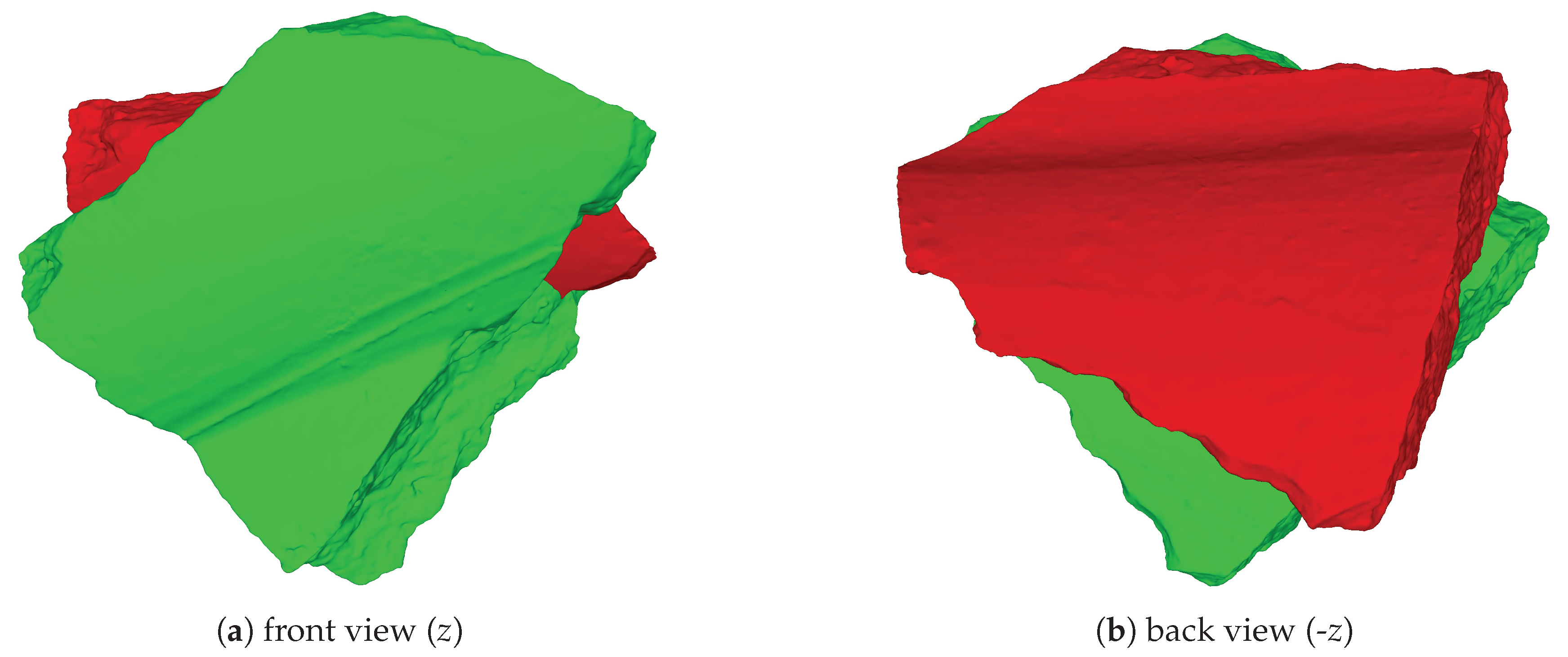
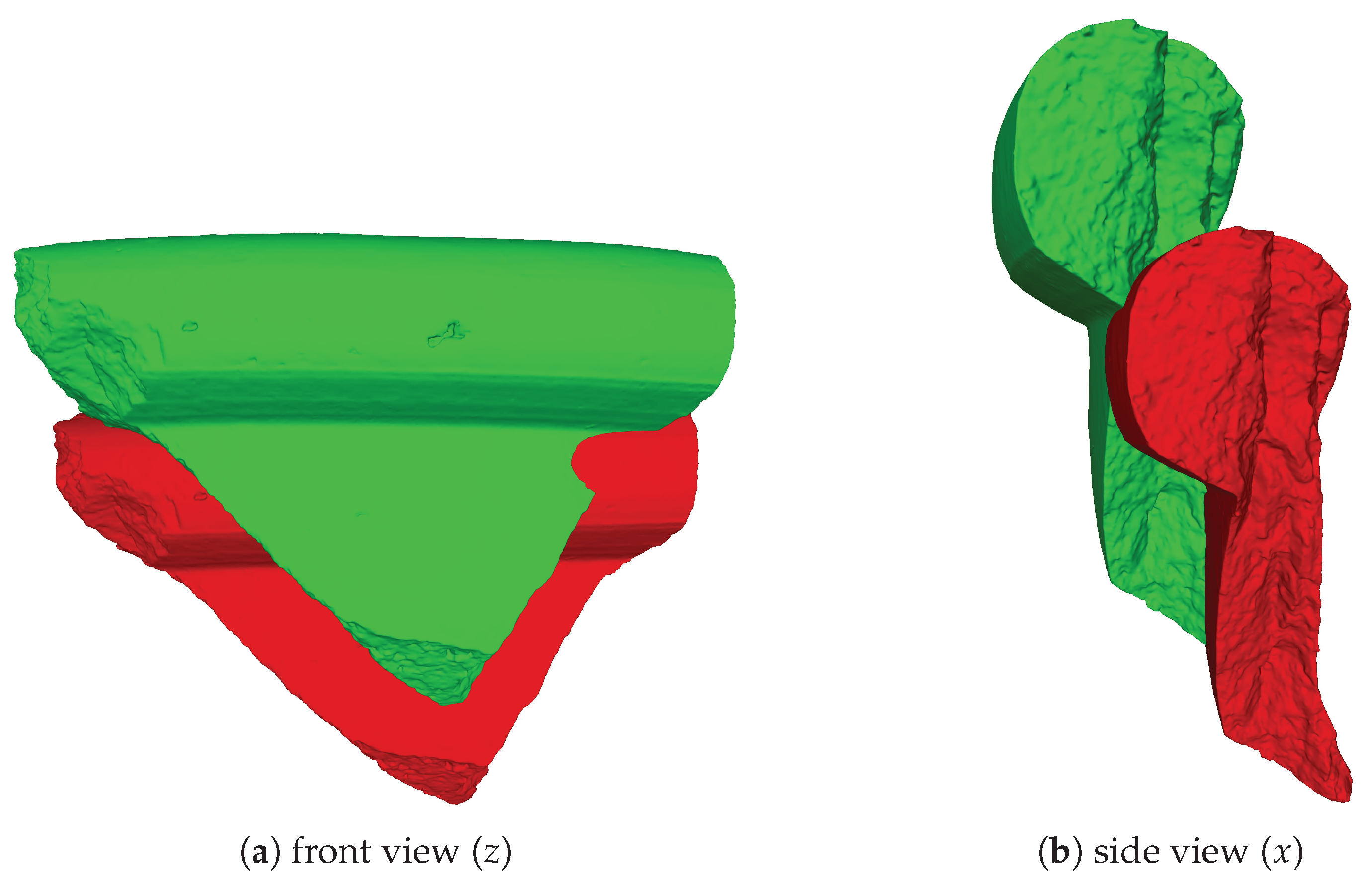
6.1. Results over the Synthetic Test Set
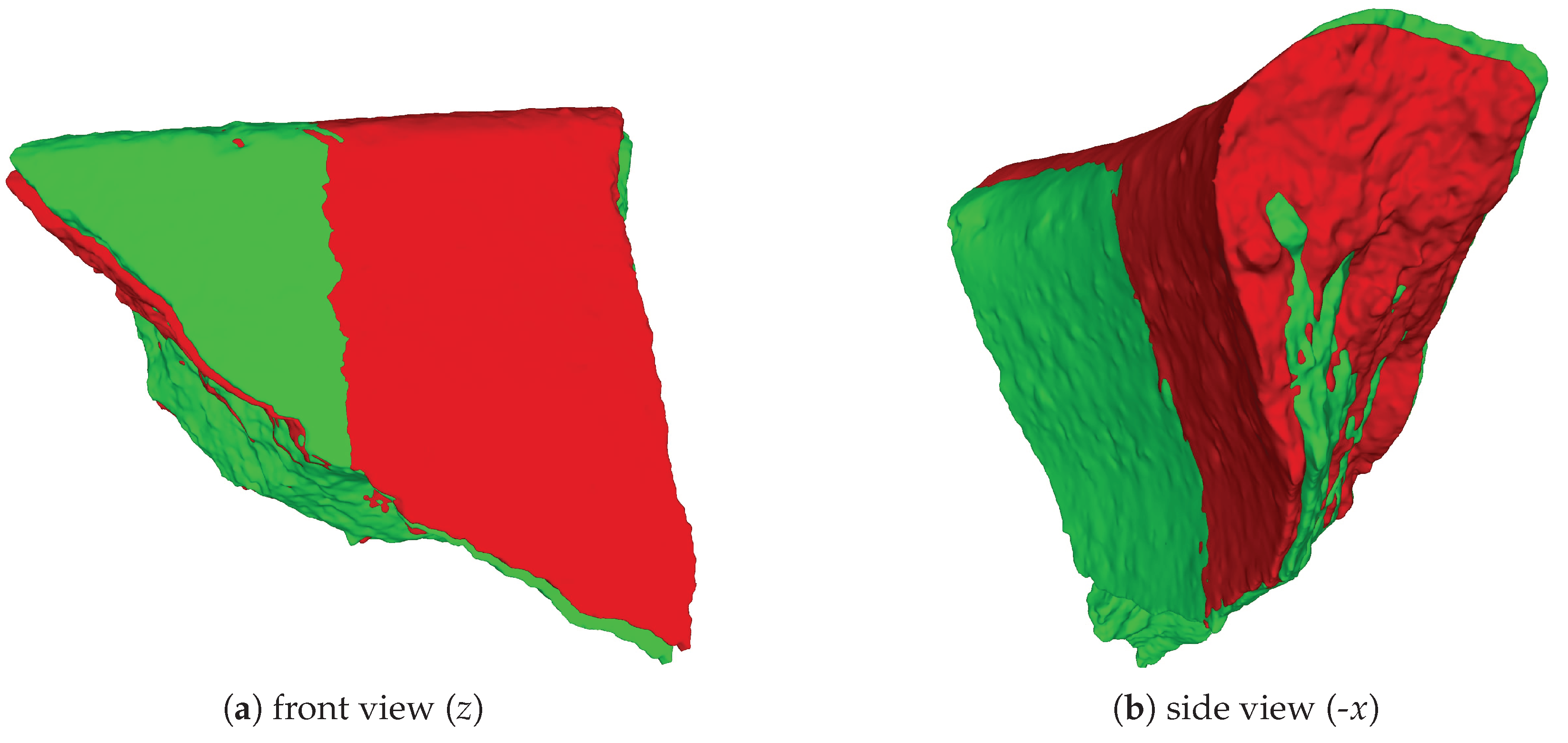
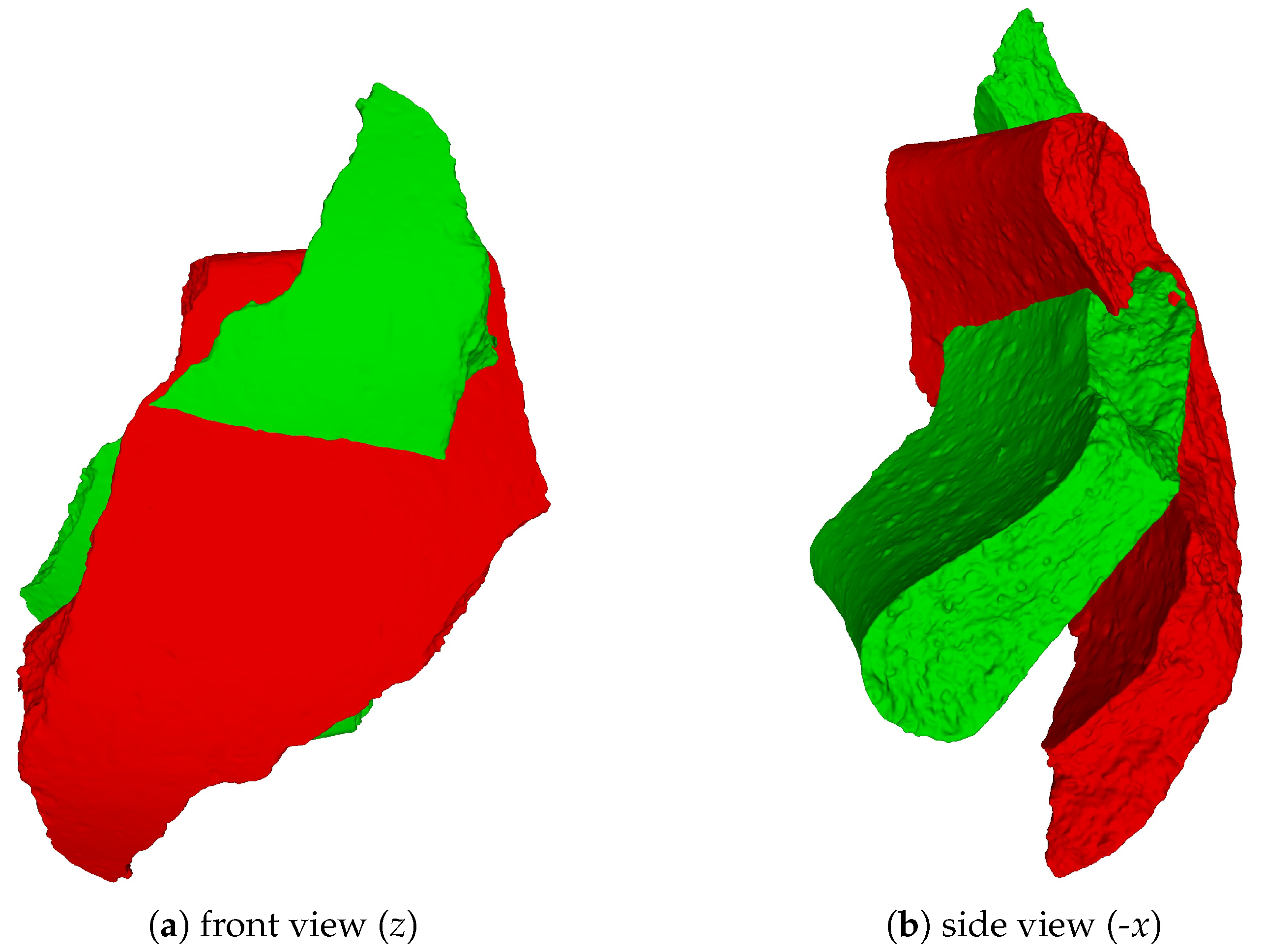
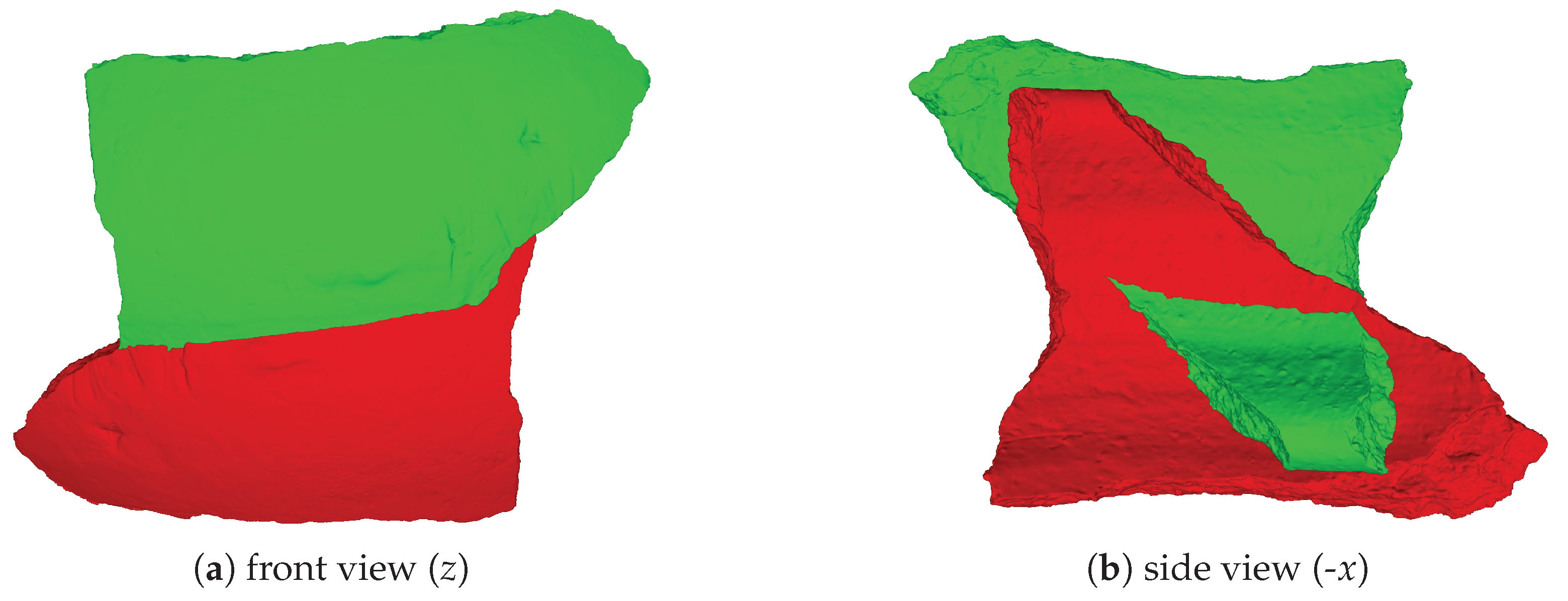
6.2. Results over the Real-World Test Set
7. Conclusion
Funding
Data Availability Statement
Acknowledgments
Conflicts of Interest
Appendix A
Appendix A.1

| Vessel | Train | Test | Total |
|---|---|---|---|
| LV | 78,892 | 8,695 | 87,587 |
| MV | 76,664 | 7,816 | 84,480 |
| SV | 77,377 | 7,694 | 85,071 |

| 1 | Here, we use the right-handed coordinate system as our reference coordinate system with the y axis pointing up, coinciding with the rotation axis. |
References
- Andrews, S.; Laidlaw, D.H. Toward a framework for assembling broken pottery vessels. AAAI/IAAI 2002, 945–946. [Google Scholar]
- Arun, K.S.; Huang, T.S.; Blostein, S.D. Least-squares fitting of two 3-d point sets. IEEE Transactions on pattern analysis and machine intelligence 1987, 698–700. [Google Scholar] [CrossRef] [PubMed]
- Cohen, F.; Zhang, Z.; Liu, Z. Mending broken vessels a fusion between color markings and anchor points on surface breaks. Multimedia Tools and Applications 2016, 75, 3709–3732. [Google Scholar] [CrossRef]
- Blender. Available online: http://www.blender.org (accessed on 15 July 2022).
- Cooper, D.B.; Willis, A.; Andrews, S.; Baker, J.; Cao, Y.; Han, D.; Kang, K.; Kong, W.; Leymarie, F.F.; Orriols, X. Assembling virtual pots from 3d measurements of their fragments. In Proceedings of the 2001 conference on Virtual reality; 2001; pp. 241–254. [Google Scholar]
- Corsini, M.; Cignoni, P.; Scopigno, R. Efficient and flexible sampling with blue noise properties of triangular meshes. IEEE transactions on visualization and computer graphics 2012, 18, 914–924. [Google Scholar] [CrossRef] [PubMed]
- Trimesh. Available online: https://trimsh.org/ (accessed on 15 July 2022).
- Di Angelo, L.; Di Stefano, P.; Guardiani, E. A review of computer-based methods for classification and reconstruction of 3d high-density scanned archaeological pottery. Journal of Cultural Heritage 2022, 56, 10–24. [Google Scholar] [CrossRef]
- Eslami, D.; Di Angelo, L.; Di Stefano, P.; Guardiani, E. A semi-automatic reconstruction of archaeological pottery fragments from 2d images using wavelet transformation. Heritage 2021, 4, 76–90. [Google Scholar] [CrossRef]
- Eslami, D.; Di Angelo, L.; Di Stefano, P.; Pane, C. Review of computer-based methods for archaeological ceramic sherds reconstruction. Virtual Archaeology Review 2020, 11, 34–49. [Google Scholar] [CrossRef]
- Garland, M.; Heckbert, P.S. Surface simplification using quadric error metrics. In Proceedings of the 24th annual conference on Computer graphics and interactive techniques; 1997; pp. 209–216. [Google Scholar]
- Huang, Q.X.; Flöry, S.; Gelfand, N.; Hofer, M.; Pottmann, H. Reassembling fractured objects by geometric matching. ACM siggraph 2006 papers 2006, 569–578. [Google Scholar]
- Jylänki, J. An exact algorithm for finding minimum oriented bounding boxes. Semantic Scholar. 2015. Available online: http://clb.confined.space/minobb/minobb.html (accessed on 20 July 2023).
- Kampel, M.; Sablatnig, R. 3D puzzling of archeological fragments. Proc. of 9th Computer Vision Winter Workshop; 2004; pp. 31–40. [Google Scholar]
- Kashihara, K. An intelligent computer assistance system for artifact restoration based on genetic algorithms with plane image features. International Journal of Computational Intelligence and Applications 2017, 16, 1–15. [Google Scholar] [CrossRef]
- Kaya, G.; Bilmenoglu, C. Accuracy of 14 intraoral scanners for the all-on-4 treatment concept: a comparative in vitro study. J Adv Prosthodont 2022, 14, 388–398. [Google Scholar] [CrossRef] [PubMed]
- Kim, K.; Hong, J., Rhee. Reconstructing the past: Applying deep learning to reconstruct pottery from thousands shards. In Machine Learning and Knowledge Discovery in Databases. Applied Data Science and Demo Track: European Conference, ECML PKDD 2020, Ghent, Belgium, September 14–18, 2020, Proceedings, Part V; 2021; pp. 36–51. [Google Scholar]
- Kingma, D.P. Adam: A method for stochastic optimization. arXiv 2014, arXiv:1412.6980 2014. [Google Scholar]
- Lee, S.; Yang, Y. Progressive deep learning framework for recognizing 3d orientations and object class based on point cloud representation. Sensors 2021, 21, 6108. [Google Scholar] [CrossRef] [PubMed]
- Malischewski, S., Schumann, H., Hoffmann, D. Kabsch algorithm. Available online: https://biomolecularstructures.readthedocs.io/en/latest/kabsch/ (accessed on 20 July 2023).
- Marie, I.; Qasrawi, H. Virtual assembly of pottery fragments using moiré surface profile measurements. Journal of Archaeological Science 2005, 32, 1527–1533. [Google Scholar] [CrossRef]
- Mark, d.B., Otfried, C., Marc, v.K., Mark, O. Computational geometry algorithms and applications, 3rd ed.; Springer Science & Business Media: Berlin, Germany, 2008; pp. 147–171. [Google Scholar]
- Pymeshlab. Available online: https://pymeshlab.readthedocs.io/en/latest/ (accessed on 21 July 2023).
- O’Rourke, J. Finding minimal enclosing boxes. International journal of computer & information sciences 1985, 14, 183–199. [Google Scholar]
- Palmas, G., Pietroni, N., Cignoni, P., Scopigno, R. A computer-assisted constraint-based system for assembling fragmented objects. Digital Heritage International Congress (Digital-Heritage), IEEE; 2013; pp. 529–536. [Google Scholar]
- Papaioannou, G., Karabassi, E.A., Theoharis, T. Theoharis, T. Automatic reconstruction of archaeological finds – a graphics approach. International Conference on Computer Graphics and Artificial Intelligence; 2000; pp. 117–125. [Google Scholar]
- Qi, C.R., Su, H., Mo, K., Guibas, L.J. Pointnet: Deep learning on point sets for 3d classification and segmentation. In Proceedings of the IEEE conference on computer vision and pattern recognition; 2017; pp. 652–660. [Google Scholar]
- Ronnegren, J. Real time mesh fracturing using 2d voronoi diagrams. Bachelor of Science in Digital Game Development, Blekinge Institute of Technology, Karlskrona, Sweden, 20 June 2020. [Google Scholar]
- Ruder, S. An overview of gradient descent optimization algorithms. arXiv 2016, arXiv:1609.04747 2016. [Google Scholar]
- Sakpere, W. 3D reconstruction of archaeological pottery from its point cloud. In Pattern Recognition and Image Analysis: 9th Iberian Conference, IbPRIA 2019, Madrid, Spain, July 1–4, Proceedings, Part I 9; Springer, 2019; pp. 125–136. [Google Scholar]
- Stamatopoulos, M.I.; Anagnostopoulos, C.N. 3D digital reassembling of archaeological ceramic pottery fragments based on their thickness profile. arXiv 2016, arXiv:1601.05824 2016. [Google Scholar]
- Straumann. Available online: https://www.straumann.com/clearcorrect/br/pt/discover/virtuo-vivo.html (accessed on 11 February 2025).
- Van Loan, C.F. Generalizing the singular value decomposition. SIAM Journal on numerical Analysis 1976, 13, 76–83. [Google Scholar] [CrossRef]
- Zheng, S., Huang, R., Li, J., Wang, Z. Reassembling 3D thin fragments of unknown geometry in cultural heritage. ISPRS Annals of the Photogrammetry, Remote Sensing and Spatial Information Sciences 2014, 2, 393–399. [Google Scholar]
- Zhou, Y., Barnes, C., Lu, J., Yang, J., Li, H. On the continuity of rotation representations in neural networks. In Proceedings of the IEEE/CVF Conference on Computer Vision and Pattern Recognition; 5753; pp. 5745–5753. [Google Scholar]
| Layer type | Output Shape | Parameters |
|---|---|---|
| Input | 3 | 0 |
| Conv 1D 1×3 / 64 + ReLU | 64 | 256 |
| Conv 1D 1×64 / 64 + ReLU | 64 | 4160 |
| Conv 1D 1×64 / 64 + ReLU | 64 | 4160 |
| Conv 1D 1×64 / 128 + ReLU | 128 | 8320 |
| Conv 1D 1×128 / 1024 + ReLU | 1024 | 132096 |
| Global Max Pooling 1D | M | 0 |
| Dense 512 | 512 | |
| Batch Normalization | 512 | 2048 |
| ReLU | 512 | 0 |
| Dense 256 | 256 | 131328 |
| Batch Normalization | 256 | 1024 |
| ReLU | 256 | 0 |
| Dropout | 256 | 0 |
| Dense N | N | |
| Linear | N | 0 |
| RMSE | RMSE (x,y,z) | STD | |
|---|---|---|---|
| LV | 0.025 | (0.01, 0.021, 0.009) | 0.001 |
| MV | 0.017 | (0.008, 0.014, 0.007) | 0.0004 |
| SV | 0.013 | (0.008, 0.009, 0.006) | 0.0002 |
| RMSE | RMSE (x,y,z) | STD | |
|---|---|---|---|
| LV | 0.034 | (0.009, 0.026, 0.017) | 0.0006 |
| MV | 0.019 | (0.007, 0.01, 0.012) | 0.0002 |
| SV | 0.023 | (0.01, 0.012, 0.013) | 0.0003 |
| sherd | RMSE | RMSE (x,y,z) | STD | |
|---|---|---|---|---|
| LV29 | 0.023 | (0.013, 0.014, 0.013) | 0.0002 | |
| best cases | MV11 | 0.017 | (0.012, 0.011, 0.005) | 0.0001 |
| SV14 | 0.019 | (0.013, 0.012, 0.006) | 0.0002 | |
| LV23 | 0.034 | (0.024, 0.021, 0.013) | 0.0005 | |
| average cases | MV19 | 0.032 | (0.015, 0.025, 0.012) | 0.0005 |
| SV21 | 0.027 | (0.015, 0.02, 0.009) | 0.0004 | |
| LV21 | 0.038 | (0.026, 0.025, 0.012) | 0.0008 | |
| worst cases | MV17 | 0.038 | (0.028, 0.023, 0.011) | 0.0008 |
| SV11 | 0.033 | (0.023, 0.022, 0.01) | 0.0006 |
Disclaimer/Publisher’s Note: The statements, opinions and data contained in all publications are solely those of the individual author(s) and contributor(s) and not of MDPI and/or the editor(s). MDPI and/or the editor(s) disclaim responsibility for any injury to people or property resulting from any ideas, methods, instructions or products referred to in the content. |
© 2025 by the authors. Licensee MDPI, Basel, Switzerland. This article is an open access article distributed under the terms and conditions of the Creative Commons Attribution (CC BY) license (http://creativecommons.org/licenses/by/4.0/).


