Machine Learning Strategies for Forecasting Mannosylerythritol Lipid Production in Fermentation Processes

1. Introduction

Fermentations are, in general, inherently complex biological processes for the production of valuable compounds, characterized by interactions among various intrinsic and extrinsic variables. Intrinsic factors, such as metabolism, genetic variability, and cellular responses, interact dynamically with extrinsic variables, such as nutrient availability, pH, and oxygen levels, influencing the dynamics and output of the process. These variables are often interdependent and can vary over time, making fermentation processes unpredictable and challenging to control. This complexity impacts the consistency and efficiency of consecutive process batches, leading to variability in yield and quality. As a result, there is a demand for advanced strategies to enable real-time monitoring, modelling, and consequent optimization of processes. Such improvements are essential to enhance reproducibility and increase productivity, ultimately leading to cost efficiency, which is essential for scaling these bioprocesses to industrial scale. The large volumes of data that can be generated during fermentation bioprocesses, from online monitoring and offline sampling, present a still underexplored opportunity to develop data-driven models, such as those based on machine learning (ML), which in turn can be used to better understand the process and improve its predictability, contributing to higher process efficiency.

Fermentation bioprocesses have historically been used for food production and conservation, to improve taste, and texture [1]. In recent years, precision fermentation has attracted significant interest as a sustainable method to produce high-value ingredients, such as proteins, vitamins, and other bioactive compounds, for the alternative protein industry [2]. Beyond food, fermentation technologies have been widely developed for the production of biofuels, industrial chemicals, and pharmaceutical products [3]. Among these various fermentation products, biosurfactants have emerged as a promising class of biomolecules due to their unique physicochemical properties and broad industrial applications, including the cosmetic, cleaning, and pharmaceutical industries [4].

Surfactants are molecules that reduce surface or interfacial tension between liquids, a liquid and a gas, or a liquid and a solid, and are used extensively across various industries. Synthetic surfactants, mostly produced by the petrochemical industry, are commonly used, but present several concerns regarding toxicity as they affect the microbial world, soil, plants, and aquatic life [5]. With environmental issues becoming a pressing concern for both the public and industry, there is an urgent need to identify greener, more sustainable alternatives to petrochemical surfactants. Biosurfactants offer an appealing solution, as they are naturally derived and produced as secondary metabolites by bacteria or fungi, making their production more environmentally friendly and sustainable [6].

Mannosylerythritol lipids (MELs), a type of glycolipid compounds, are among the most interesting biosurfactants. MELs are surface-active agents with hydrophobic and hydrophilic moieties that allow them to reduce surface and interfacial tension [7]. The hydrophobic moieties that compose these molecules consist of a mannose and an erythritol, specifically 4-O-$\beta$-D-mannopyranosyl-meso-erythritol, and the hydrophilic moiety is composed of fatty acids and acetyl groups [8]. Their exceptional surface-active properties, versatile biochemical functions, non-toxicity, biodegradability, environmental compatibility, among other attributes, make MELs an interesting potential option for various applications [8].

Despite the advantage of using MELs or other biosurfactants instead of current less environmentally friendly alternatives, their production remains economically challenging [9]. This can be attributed to low product yields, high production costs, and the complex interplay of process variables that influence biosurfactant synthesis. These challenges emphasize the need to optimize production processes to enhance their viability for commercialization and industrial adoption [9]. This is, in general, a common problem for most biosurfactants, since their production is affected by a variety of factors, such as the carbon [10] and nitrogen source used [11], the consequent carbon-to-nitrogen ratio [12], and abiotic factors such as temperature, oxygen [13] and pH [14], among others. Moreover, the high variability in the production process makes it challenging to predict the success of each fermentation run. This challenge is further amplified when using agro-industrial residues, such as residual oils or cheese whey [15], due to their possible variable composition.

Due to the many variables involved in biosurfactant production, testing each factor individually is both time-consuming and expensive. A more efficient approach gaining popularity is the use of data-driven models, like machine learning. These models can analyse past data to extract insights and predict outcomes, without needing prior knowledge of the reaction mechanisms. This emerging approach could lead to new technologies that optimize fermentation processes and reduce the production costs of biosurfactants. Although the application of machine learning in bioengineering is still in its early stages, several studies have already demonstrated the potential of these models to predict biological processes, using unsupervised [16] and supervised learning approaches [17].

Neural Networks (NN) are the most common models used in the field of ML applied to bioreactors, to predict product concentration as they are very flexible due to the several possible adjustable parameters and topologies [18]. The use of NN dates back to 1990 when Thibault et al. [19] used a fairly simple NN, with only one hidden layer, to predict the concentration of cells and substrate at the next sampling interval, in a continuously stirred bioreactor, by giving the algorithm the dilution rate, concentration of cells and substrate at the current sampling interval, achieving fairly accurate predictions. It is worth noting that NN was used to predict simulation results and was not applied to a real-world case. More recently, Zhang et al. [20], also used a NN to successfully predict the concentrations of biomass for two strains of Clostridium butyricum, glycerol and 1,3-propanediol in both batch and fed-batch mode in a 5L bioreactor. By using a double-input NN the predictions were successful for the fermentation process for strain I of Clostridium butyricum but failed for strain II. After adjusting the model by adding two more input variables, the model reduced its error rate, but the predictions for strain II were still significantly different from reality.

Another popular model is random forests (RF) since they are fairly simple to implement and provide high accuracy, even for small data sets. RF possess several parameters that can be adjusted as needed, such as the number of trees, and the maximum depth of each tree, to name a few [21]. Zhang et al. [22] used two ML models - RF and gradient boost regression - to optimise and predict bio-oil production from hydrothermal liquefaction of algae. In this study, although the gradient boosting regression model outperformed RF, the model still achieved a coefficient of determination (R²) of approximately 0.90, successfully predicting oil yield, oxygen, and nitrogen content.

Although there are quite a few studies in which ML techniques are applied to forecast product concentration in bioreactors, there are only a handful of studies that have focused specifically on biosurfactant production. Among the few studies, Jovic et al. [23], forecasted the biosurfactants yield, emulsification index (E24), and surface tension reduction using a support vector machine (SVM). Similarly and more recently, Bustamante et al. [24] predicted biosurfactant concentration, E24, and surface tension reduction for biosurfactant production, both in Erlenmeyer and bioreactors, using a NN model. To the best of our knowledge, no studies have been published on the use of ML algorithms to optimise MELs production process.

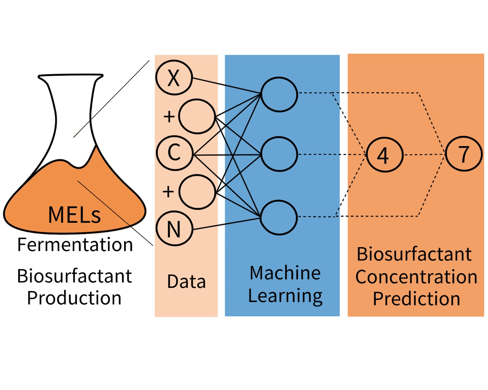
In this work, three different ML models (NN, SVM, and RF) were tested to predict MELs concentration in the cultivation ofMoesziomyces spp. in Erlenmeyer flasks.

This work aims to enhance the predictability and efficiency of MELs production by applying ML models. These models are expected to anticipate fermentation outcomes, enabling corrective actions to adjust the process trajectory or terminate unsuccessfully batches earlier. This approach has the potential to improve process consistency and reduce costs.

2. Materials and Methods

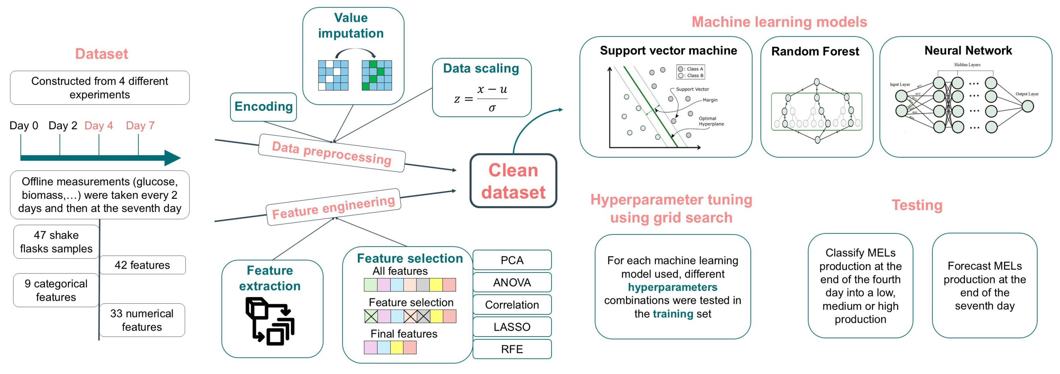
Figure 1 showcases a simplified workflow of the methodology used in this work, further detailed in the next sections.

2.1. Dataset

The dataset used in this study was compiled from four different groups of experiments previously carried out by the research group [15,25,26,27,28], with the aim of producing MELs.

In all experiments, the concentrations of biomass, carbon, and nitrogen concentrations were assessed at the beginning of the experiment (day 0), day 2, day 4, day 7, and, for longer experiments, days 10, 14, and 18. Furthermore, MEL and lipid concentrations were measured on days 4 and 7, and, for longer experiments, at days 10, 14, and 18. Possible carbon sources, both hydrophilic (glucose, glycerol, cheese whey or no carbon sources) and hydrophobic (soybean oil, fish oil, sunflower oil, rapeseed oil, and waste frying oil), constitute categorical variables. Sodium nitrate was consistently used as the nitrogen source. The final dataset is composed of 47 samples, with each shake flask run considered a sample, and includes 42 features. Although the experiments aimed at the production of MELs, they followed different strategies, varying in the carbon source used, feeding strategy, initial biomass, headspace volume, carbon-to-nitrogen ratio, and duration. The shortest experiment was concluded after 7 days of fermentation, while the longest experiment was extended to 18 days. Figure S1 (Supplementary Material, Figure S1) shows the evolution of biomass throughout the first 7 days for all experiments. Figure S2 (Supplementary Material, Figure S2) and Figure S3 (supplementary material, Figure S3) depicts the consumption of carbon and nitrogen, respectively, throughout the first 7 days for all experiments.

-

Experiment 1 includes 18 samples, a duration of 18 days and a volume of 50 mL. D-Glucose, glycerol (or simply no hydrophilic carbon source) were used in combination with hydrophobic carbon source, such as soybean oil,rapeseed oil and waste frying oil.

-

Experiment 2 includes 10 samples, a duration of 10 days, and a volume of 50 mL. Waste frying oil was used as the hydrophobic carbon source, while D-glucose and cheese whey were used as hydrophilic carbon source.

-

Experiment 3 comprises 8 samples, a duration of 7 days, and consistent use of D-glucose and waste frying oil as hydrophylic and hydrophobic carbon sources, respectively. Four different volumes were tested (200 mL, 100 mL, 50 mL, and 25 mL), with each conditions run in duplicate.

-

Experiment 4 includes 11 samples, each running for 10 days with a volume of 50 mL. D-Glucose was used as the hydrophilic carbon source, while the hydrophobic carbon sources varied between residual fish oil and sunflower oil.

2.2. Data Preprocessing

After assembling the dataset, data preprocessing was required before testing the ML models. As previously stated, the dataset consists of both numerical and categorical features. To use the categorical features as inputs, they were encoded in numerical values using one hot encoding technique was applied, where each categorical feature was represented by 0 for absence and 1 for presence [29]. For example, if glucose was used in a sample, it would be represented by 1 while all other carbon sources would be represented by 0.

Additionally, the dataset contained some missing values that were not due to the different experiment durations but rather to normal experimental unexpected experimental issues. Therefore, value imputation was necessary for the analysis, as most models cannot handle missing data. To select the most appropriate imputation method, 5% of the known values of the dataset were randomly removed, and then several methods were used to predict the removed values. These methods included simple and commonly used techniques, such as the mean and median, as well as machine learning algorithms like k-Nearest Neighbour, RF, Decision Tree (DT), Bayesian Ridge, and SVM. The performance of each method was assessed by comparing the mean squared error (MSE) [30]. Analysing the results obtained from the different methods, the k-Nearest Neighbour Regressor with two neighbours, achieved the lowest MSE (42.16). Therefore, it was selected to impute the true missing values in the dataset.

After completing this step, the data was scaled, as not all features have the same order of magnitude. Scaling the data ensures that each variable contributes equally to the analysis. The z-score method was applied, which standardizes each feature to have a mean of zero and a standard deviation of one [31]. After scaling, 80% of the data (37 samples) was used for training and the remaining 20% for testing (10 samples) the classifiers.

2.3. Feature Engineering

After completing data preprocessing, new features were extracted from the original ones, to provide additional information not directly available in the initial feature set. The carbon/nitrogen ratio for each day was calculated and added as a new feature. Next, based on knowledge of the process, the biomass growth rate, $\mu$, was calculated with Equation (1), where $X_v$ represents the biomass concentration at time t, and $X_{v_0}$ represents the initial biomass concentration.

$$X_v=X_{v_0}\times e^{\mu t}$$

(1)

Glucose and nitrogen consumption rates were calculated by subtracting the final concentration from the initial concentration (day 0) and then dividing by the total duration of the experiment. The biomass/substrate yield was calculated by dividing the biomass concentration at the end of the experiment by the substrate consumption throughout the days. Moreover, the specific rate of nitrogen and glucose consumption were also calculated using Equation (2). In Equation (2), S represents the glucose concentration when calculating the glucose consumption rate, and nitrogen when calculating the nitrogen consumption rate.

$$q_S={\displaystyle \frac{1}{X_v}}\times {\displaystyle \frac{dS}{dt}}$$

(2)

Finally, the increase or decrease that substrate, nitrogen, MELs and lipids concentration suffer between each day (Equation (3)) were also added as new features.

$$\Delta X_i=X_i-X_{i-1}$$

(3)

Where $\Delta X_i$ represents the change (increase or decrease) in the concentration of the variable X (e.g., substrate, nitrogen) on day i, $X_i$ represents the concentration of the variable on the current day (i) and $X_{i-1}$ represents the concentration of the variable on the previous day $i-1$.

At the end of the feature extraction process, the final dataset was composed of 47 samples and 74 features.

Feature selection methods were also applied to the dataset to ensure that only relevant information was provided to the models and to assess which features would have a greatest impact and be most relevant for MELs concentration prediction. Five different feature selection methods were tested creating therefore five different features subsets.

Principal component analysis (PCA) was the first method explored for feature selection. It creates several principal components, where each component is a linear combination of the original features.

In this work, in order to perform dimensional reduction, all principal components that explained 90% of the variance in the data were selected, and then identified how much each feature was contributing to each principal component. Afterward, the mean of the contribution of each variable was calculated, and every feature with a contribution below zero was discarded [32].

Dimensionality was also reduced using the analysis of variance (ANOVA) method. In the context of feature selection, ANOVA is used to rank the features by calculating the ratio of variances between and within groups [33,34]. Then, the same number of features previously obtained from PCA were selected from the features ranking.

The Least Absolute Shrinkage and Selection Operator (LASSO) technique was also used for feature reduction. LASSO is a regression method that incorporates a penalty term, known as L1 regularization. The L1 regularization term is the sum of the absolute values of the regression coefficients, multiplied by a tuning parameter. LASSO works by simultaneously finding the coefficient values that minimise the sum of the squared differences between predicted and actual value (the residual sum of squares) and minimising the L1 regularization term. As a result, LASSO shrinks some coefficients towards zero, which can then be used to reduce the feature set by eliminating the ones with zero coefficient [35,36].

Dimensionality reduction through the removal of correlated features was also done, using Pearson’s correlation, which measures the linear relationship between two features. Correlation values can range between -1 and 1, indicating that the features are completely correlated, negatively or positively, respectively, while 0 means there is no correlation between such features [37]. In this work, when two features had an absolute correlation greater than 60%, one of them was removed [38].

Finally, the last method used was the recursive feature elimination (RFE). This method starts with all features and recursively eliminates them based on their importance to a given estimator. In other words, a model is built and fitted with the whole set of features, and then an importance score for each feature is calculated. The least important feature is removed, and the previous process is repeated until a specific number of features is reached. The model chosen was the support vector regressor with a linear kernel [39].

The features selected by each method for day 4 are represented in Table S1 (Supplementary Material, Table S1), and Table S2 (Supplementary Material, Table S2) for day 7.

2.4. Machine Learning Techniques

Different machine learning techniques were employed to forecast MELs concentration at the end of days 4 and 7. This study used three supervised ML algorithms: Support Vector Machine, Random Forest, and Neural Network.

Real-world data often exhibits non-linear separability, making it challenging to distinguishing between classes in the original feature space and to determine the separation surface effectively. To address this challenge, kernel functions are employed to transform the data into a higher-dimensional feature space where the classes become more easily separable. Among the several existing kernels, the most common ones are linear, polynomial, radial basis function (RBF), and sigmoid. Support Vector Machine is an algorithm used for both classification and regression tasks. The SVM uses this kernel-based mapping to transform the data into a higher-dimensional space where it then searches for the optimal hyperplane that can separate the data. The construction of the hyperplane is mainly dependent on the support vectors, which are created through data points from the training set and support the margins of the hyperplane. The choice of kernel function is a key hyperparameter in the SVM since it allows the model to operate in a high-dimensional feature space without explicitly calculating the coordinates in that space. This is essential because high-dimensional spaces are often too large to compute directly, making calculations slow or even impractical for large datasets. A detailed description of the method can be found in Zhang, 2020 [40].

The Random Forest model was also used in this study. Random Forest is an ensemble learning method, a combination of several inducers, more specifically Decision Trees (DT). Each DT in the forest is a simple model that individually has low accuracy since it only uses a subset of the features. By aggregating DT, using averaging for regression or majority voting for classification, the RF algorithm can construct complex decision surfaces that effectively separate classes. One of the advantages of RF is its ability to achieve high accuracy even with limited data relative to the number of features, as it utilizes bootstrap sampling to generate diverse training subsets for each tree. More information about this model is present in Cutler, 2012 [21].

Finally, predictions were also made using a Feed-forward Neural Network (NN). Briefly, an NN is divided into three parts: input layer, hidden layers, and output layer. The NN algorithms are inspired by the neural networks present in the human brain, where an external stimulus is received and propagated by a neural network connected by synapses that process the information and return a final command. In this approach, the input data is provided to the algorithm, which will activate certain nodes (or neurons) in the input layer which will in turn activate other nodes in the hidden layers through weight connections associated with a bias. These interactions generate an output based on the connections from the input layer through the hidden layers. Training data must be provided to the algorithm so it can learn the weights that connect the various neurons, enabling accurate predictions. The weight learning process is done by backpropagation, which is a cost function minimisation through gradient descent. When test data is provided to the network it should be able to predict this new and unseen entity based on its learning from the training set [41].

This type of algorithm requires a very large dataset for training because increasing the number of layers significantly raises the number of parameters that need to be optimized.

The final step in the process was to optimise the hyperparameters of each model. Several combinations of hyperparameters were tested for each subset of features. Therefore, the combinations that produced the lower error with a certain subset may not be the best combination when applied to another subset. For the RF model, the parameters tested included the number of trees, the criterion to measure the quality of a split, the maximum tree depth, the minimum number of samples required to be at a leaf node, the maximum number of features to consider when looking for the best split and whether bootstrap samples are used when building trees. Regarding SVM, four different kernels were tested along with different values for the regularization parameter, and finally different gamma and epsilon values were also tested. Moreover, in the case of the polynomial kernel, several polynomial degrees were tested. Finally, different hyperparameters were also tested for the NN. The parameters tested were the different number of hidden layers, neurons present in those layers, and the batch size given to NN. It is also worth noting that the NN had a maximum number of epochs of 100 and had incorporated a monitor function stating that if the validation loss increased in more than 5 epochs, the training was stopped, and the best model was saved. All models were trained during this process and the weights were saved at the end of the training, so the same trained model could be applied to the testing set and results would stay consistent. The NN configuration that achieved the best result for the forecasting of day 4 had three hidden layers with 64, 32, and 16 neurons, respectively, and a single-neuron output layer. Data samples were processed in batches of eight. The loss function used was the MSE, and the learning technique applied was the adaptive moment estimation method (ADAM). As for the forecasting of day 7 the configuration of the NN consisted of 2 hidden layers with 128 and 64 neurons, an output layer with 4 neurons (the prediction is the average between the four), and a batch size of 4. The loss function used was once again the MSE and the learning technique applied the ADAM method.

To evaluate the performance of the models, two different metrics were chosen: the Mean Squared Error and the Mean Absolute Error (MAE), represented by the following equations:

$$MSE={\displaystyle \frac{1}{n}}\sum _{i=1}^n{(y_i-\widehat{y_i})}^2$$

(4)

$$MAE={\displaystyle \frac{1}{n}}\sum _{i=1}^n|\widehat{y_i}-y_i|$$

(5)

where $y_i$ and $\widehat{y_i}$ are the observed value and the predicted value, respectively.

All the code in this study was implemented in Python version 3.11.4. The SVM and the RF were done using the library scikit-learn [42] while the NN was constructed using the libraries tensorflow [43] and keras [44]. The experiments were run on a computer with an Intel i7 7th quad-core processor with GPU Nvidia 1060, and 16GB of RAM. The source code as well as the dataset are available in the GitHub MELs-forecasting (Further details in the data availability statement).

3. Results and Discussion

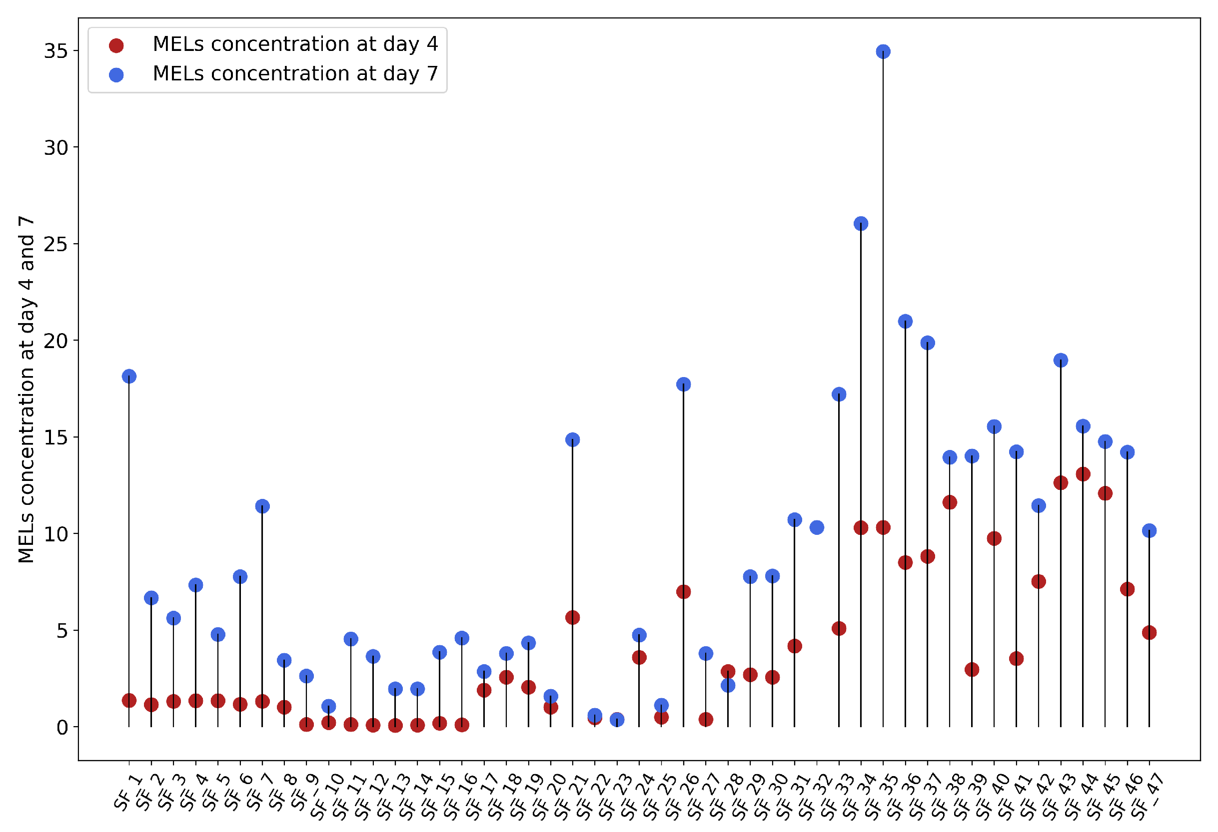
Before applying the ML workflow (Figure 1), data characterization was done. Firstly, MELs concentrations at days 4 and 7 were represented in Figure 2, showing no clear pattern between the two time points. However, when Pearson’s correlation was calculated for these two variables a value of 0.78 was obtained, revealing a strong positive correlation. Spearman’s test, which measures the strength and direction of a monotonic relation, was also used, revealing a correlation coefficient of 0.82, further reinforcing Pearson’s results. Given the established relationship between the two variables, it is reasonable to hypothesise that predicting MELs concentration on day 4 could serve as an early indicator of the outcome of day 7. This baseline could help forecast whether a particular shake flask will achieve the desired MELs concentration, allowing for a more informed decision on whether to proceed with the fermentation process or not.

As previously stated, three different machine learning models were trained to predict MELs concentration at the end of days 4 and 7, using 37 samples. Therefore, 10 samples were kept aside for testing in a different file to avoid data leakage, corresponding to a train test split of 80/20. The testing set was chosen at random to not introduce any human bias. This split ensures that the model is trained on most of the data while still being tested on a significant portion that remains unseen during training. Then, from the training set, 7 samples were chosen to serve as the validation set, while the remaining 30 samples were used to train the models. This validation set was used to assess the performance of the model on the training set.

As described in SubSection 2.4, all models were trained during the hyperparameter optimisation step. Although the models obtain a low error when asked to predict the validation set, it is important to check for their ability to generalise over unseen data.

It is also important to note that while the dataset used was relatively small, and a larger dataset could further enhance the accuracy of predictions. Table 1 shows the MSE obtained for each model using each subset of features for day 4 and in Table 2 the experimental values, predicted ones and prediction errors are presented. The same information for day 7 predictions can be found in Table 3 and Table 4.

Overall, the predictions for day 4 were more successful than those for day 7, which was not expected, since the features used for the forecasting of day 4 included only the first 2 days of fermentation. It is also worth noting, that the models benefit from the feature selection process since the lower MSE achieved by each model was when feature reduction techniques were applied.

3.1. MELS Production Forecasting: Day 4

Given the small dataset, consisting of four distinct experiments with different initial conditions, the train test split would inevitably cause the under-representation of some initial conditions, making certain samples more challenging to predict. Nevertheless, the overall results were generally satisfactory.

The results of MELs production forecasting for day 4 using the NN model combined with the correlation-derived feature subset achieved the lowest error among all tested configurations. This combination obtained an MSE of 0.69 and an MAE of 0.58 which can be considered an high accuracy. The MAE of 0.58 suggests that the average deviation of the predictions is only 0.58 $g_{MELs}/L$. A closer examination of Table 2, which compares the values predicted by each model, shows that the NN prediction errors are below 1 g/L in 9 out of the 10 samples.

The RF achieved its lowest MSE when the ANOVA feature selection method was used, with an MSE of 3.45 and an MAE of 1.49 g/L. Although the RF model’s best MSE result was higher than most of the NN model’ MSE results, it provided the most accurate MELs concentration estimate for sample 1 on day 4. The experimental value was 0.08 g/L, while the model predicted 0.14 g/L.

The SVM consistently produced MSE values around 30, regardless of the feature selection method applied. This poor performance is likely due to a mismatch between the data’s complexity and the model’s capacity to capture it. The predictions made by the SVM were extremely narrow, ranging from 1.24 g/L to 1.91 g/L, while the actual target values varied significantly from 0.08 to 13.08 g/L. This indicates that the SVM failed to identify the optimal hyperplane to separate the data and instead settled on a region in the feature space that poorly represents the true relationship between the features and the target variable.

The success of the NN can be attributed to its capacity to capture non-linear relationships within the data and its adaptive learning method. Furthermore, the NN also benefited from the feature reduction techniques since, when comparing the MSE obtained using all the features to that achieved after removing the correlated features, there was a 61% reduction.

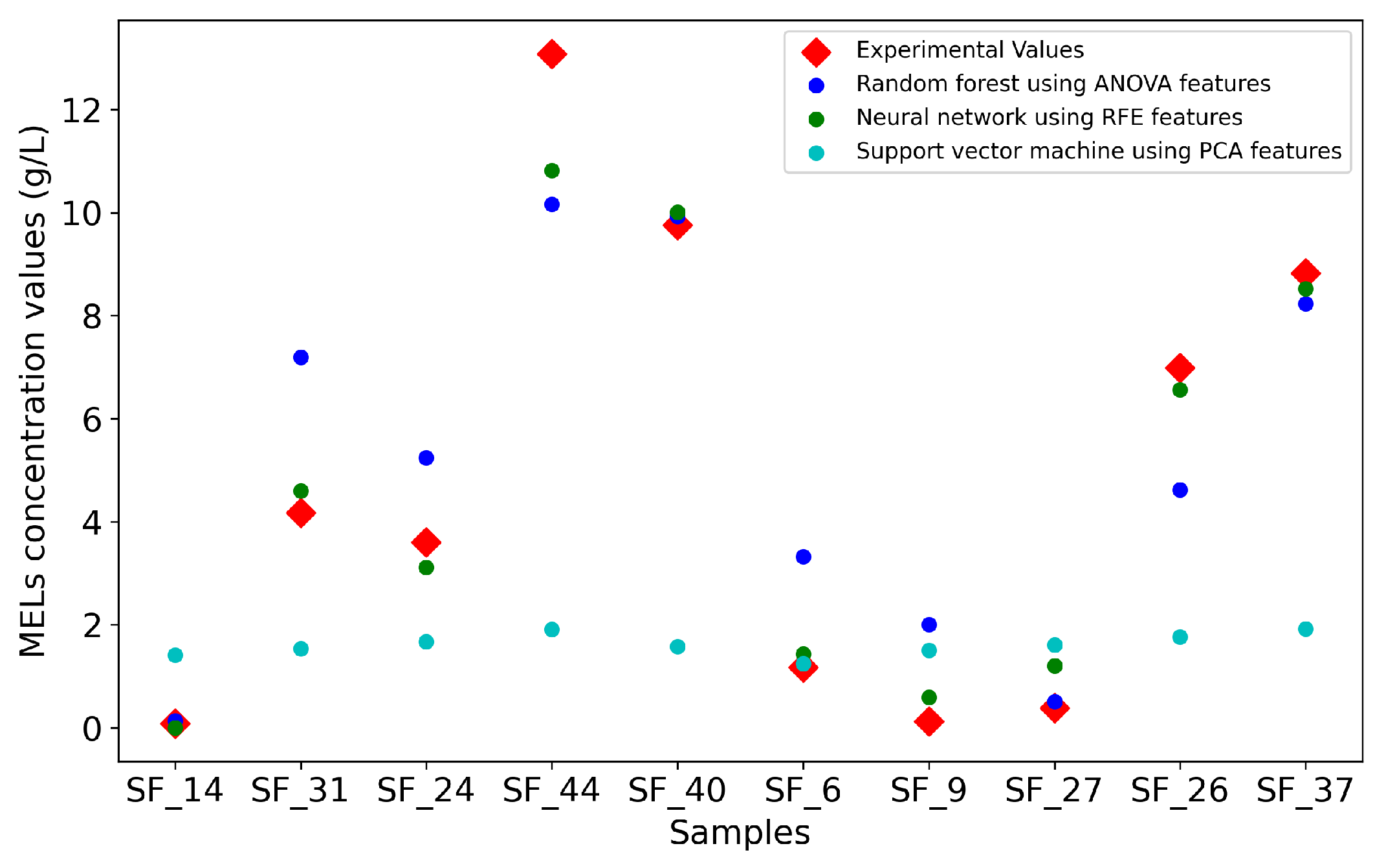
Figure 3 is a visual representation of the predictions made by the three models, highlighting their overall accuracy in forecasting the experimental values. The plot further supports the earlier observations regarding the performance of the models. Interestingly, sample 44, not only poses a forecasting challenge for the NN, but also to the RF, potentially due to the small size of the dataset, causing the under-representation of some initial conditions, which can lead to difficulties in the forecasting.

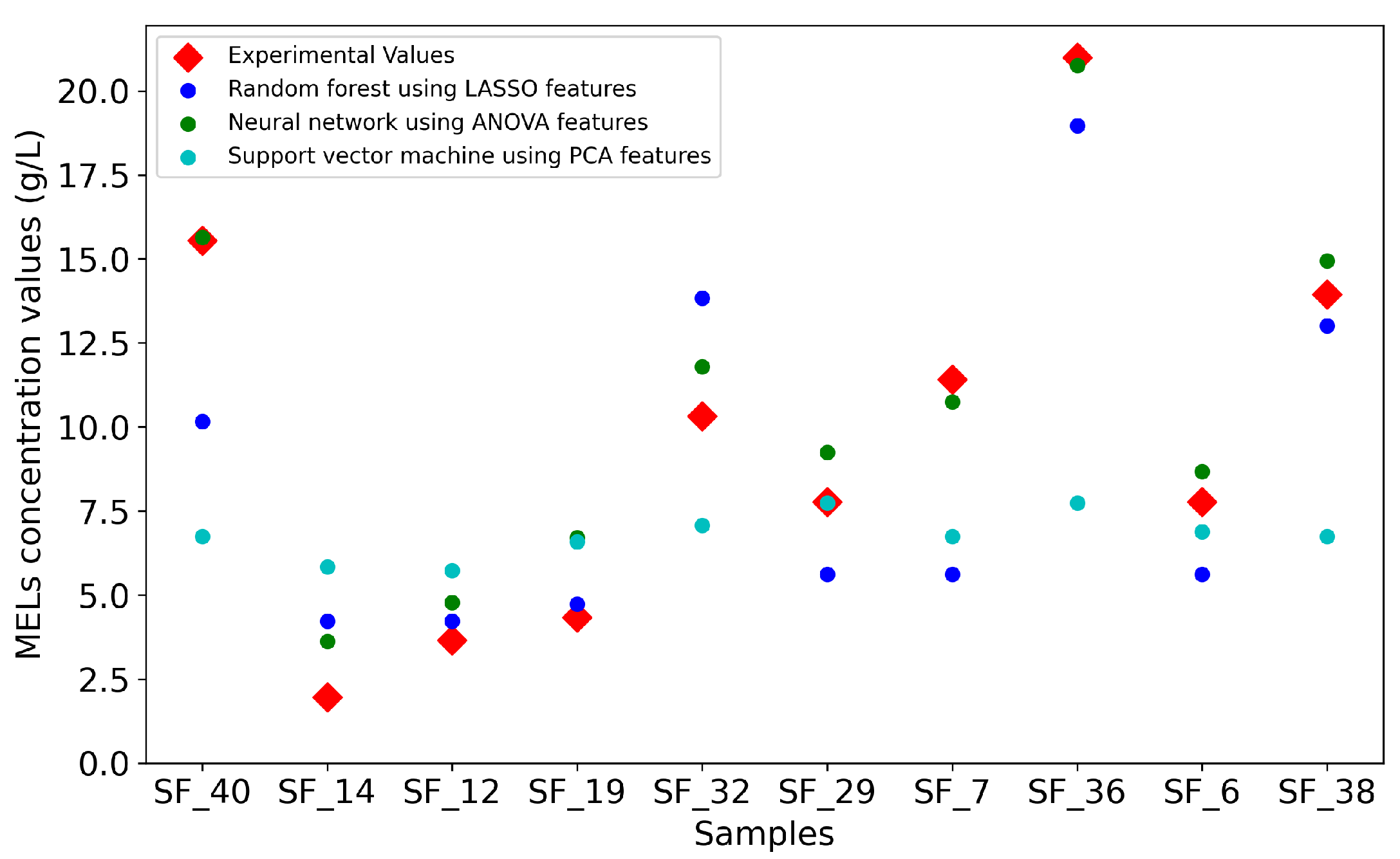
3.2. MELS Production Forecasting: Day 7

After estimating MELs production on day 4, the prediction of the concentration of MELs was carried out on day 7, the last time point common to all experiments in the dataset. As shown in Table 3, the NN model demonstrates superior performance, consistently outperforming the other models. The model achieved the lowest MSE using the feature subset selected by ANOVA with an MSE of 1.63 and an MAE of 1.1 g/L, meaning that the average deviation of the predictions from the experimental values was approximately 1 $g_{MELs}/L$. Furthermore, an analysis of Table 4 reveals only a prediction with an error greater than 2 g/L.

The RF models’ performance declined when forecasting MELs production for day 7, with the lowest MSE achieved being 9.48. Furthermore, the predictions made revealed that the RF model presented only 7 distinct values. This lack of variability likely results from the RF models’ decision trees grouping testing samples into identical nodes, leading to limited differentiation between predicted values. This may occur because the testing samples are assigned to the same leaf nodes when passing through the trees.

The SVM model performance for day 7 is similar to day 4, with high MSEs and a narrow prediction range. The model failed to find the optimal hyperplane to separate the data, even when tested with different kernels.

The NN model achieved its best result for both days 4 and 7 when the ANOVA-derived feature subset was used. This method selects features based on significant differences between independent groups, more specifically, by calculating the ratio of variance between and within groups. This approach takes into consideration the target value when applied, which can enhance the NN’s ability to learn patterns within the data. The success of the neural network across this work can be attributed once again to its robustness and flexibility.

Finally, Figure 4, reinforces the previous conclusions about the three models, but also shows that the NN model struggles to forecast sample 14 and sample 32. Once again, the dataset used in this work comprises four different experiments with different initial conditions such as different carbon and lipid sources. As a result, some initial conditions appear less frequently than others, which can impact the models’ performance due to the limited number of examples available for learning during training. For example, sample 14 initial conditions were glucose for the hydrophilic carbon source and rapeseed oil for the hydrophobic source. Rapeseed oil was only used in 6 out of 47 samples, resulting in this hydrophobic source to be under-represented in the learning set.

The predictions for day 4 were more successful than those for day 7, likely due to the non-linear relationship between the variables and the different ways MELs production depends on specific features at each time point. For day 4, MELs production may have been more strongly influenced by a particular feature present in the dataset, simplifying the prediction task. In contrast, by day 7, the relationship between MELs production and the available features may have shifted or become more complex, reducing the models’ ability to accurately capture the dynamics of the process.

3.3. Benchmarking

As previously mentioned, although ML techniques have not yet been applied to forecast MELs concentrations, some studies have focused on predicting biosurfactant production. Unfortunately, none of the existing articles published their code or dataset. In the work of Jovic et. al [23], the authors predict the biosurfactant concentration achieving a test root mean squared error (RMSE) of 0.53, which improved to 0.31 after applying the firefly algorithm. The authors also calculated the R² for their test predictions achieving a value of 0.98 before applying the firefly algorithm and 0.99 after. To enable comparison, the R² values for the best result of each model and each day in the present study were also calculated and are presented in Table 5. It is also important to note that Jovic et al. did not provide information about the size of the dataset or the inputs given to the model. To ensure the reproducibility of the results, the methodology used in the present study has been made publicly available.

A different study [24], also explored forecasting biosurfactant concentrations using NN. The authors provided information about the input features used and used particle swarm optimisation to optimise the weights and bias of the NN. This work was able to achieve a R² of 0.94, which is in line with the values obtained in our study.

Finally, Ahmad et al [45], used a NN to predict biosurfactant yield. The authors used a dataset with 27 samples, with 19 used to train the model, 4 for validation, and 4 for testing. Similarly to the previously mentioned work na R² of 0.94 was achieved for the testing set and an RMSE of 1.22. However, the authors noted that the weights varied with each run of the NN, resulting in inconsistent outcomes. In contrast, in the present work, all model weights are saved after training to ensure reproducibility and consistency in the results.

4. Conclusions

Mannosylerythritol lipids are high-value biosurfactants with diverse industrial applications, yet their production processes remain suboptimal and more costly than conventional surfactants derived from the petrochemical industry. One of the factors behind these limitations is the complexity of microbial fermentations. To accelerate bioprocess development/optimisation we envision machine learning and data-driven models playing a crucial role as they can tackle large datasets, potentially avoiding the need for several rounds of individual parameter testing and improving overall process understanding and control. ML models can also allow the detection of deviations from the expected fermentation trajectories and, the identification of early signs of contamination, equipment failure, or experimental errors. This allows for timely corrective actions, preventing batch failures before they occur or stopping a potentially failed process saving time and reducing costs. A critical first step towards achieving this is the establishment of models capable of predicting fermentation performance, in this work the final MELs concentration, relying solely on early-stage data.

In this study, we presented MELs concentration forecasting on days 4 and 7 of the fermentation process using three different ML models and applying several dimensionality reduction techniques. Between the three ML models tested, the neural network had the best performance both for day 4 and day 7 prediction, especially when coupled with feature selection techniques.

The results for day 4 were quite impressive as the models were being fed solely with data from days 0 and 2 and achieved an average deviation from the experimental value of 0.58 g/L and a R² of 0.96 which indicates that the model is well fitted for the data. The ability to forecast MEL concentration for day 7 with data from the first 4 days of fermentation is quite promising as an early batch quality assessment metric. Considering that the average deviation from the experimental values was nearly 1 g/L, at day 4, production could be stopped avoiding more resource waste and reducing its associated costs.

This work presents a significant contribution to the field of MELs production and fermentation bioprocess development as there are still few reported examples of the application of ML techniques to forecast production outcomes. Moreover, the work here presented aims to be a foundation for a more transparent and open development of such forecasting tools. The framework here demonstrated can also be directly used for other datasets and adapted with minimal modifications to address different problems, such as bioprocesses with other microbial or animal cell types. Future work opportunities include the use of bioreactor data to improve process predictability. Such advancements could play an important role in broader industrial applications and more efficient biomanufacturing systems.