Submitted:
12 February 2025
Posted:
12 February 2025
You are already at the latest version
Abstract
The presence of oil films in the ocean poses a significant environmental challenge for companies engaged in primary oil processing on offshore platforms. During crude oil treatment, residual water containing oils and greases (TOG) is discharged back into the ocean, potentially leading to the formation of oil films. The interaction between TOG levels and meteoceanographic variables — including wind direction (WD), wind speed (WS), current direction (CD), current speed (CS), wind wave direction (WWD), and peak period (PP) — influences the formation and satellite detection of these films. This study investigates the impact of these factors on the occurrence, detection, and extent of oil films using various statistical classifiers. Key findings reveal that Random Forest outperformed other classifiers, achieving an area under the ROC curve of 0.93. The combined use of classifiers, multivariate techniques, desirability analysis, and Design of Experiments (DOE) proved highly effective. Higher values of WS, WD, and CS were associated with a lower likelihood of oil film occurrence and detection, whereas higher TOG, PP, WWD, and CD values increased this probability. CS and TOG positively contributed to the extent of oil films, while high WS values reduced it. These results provide a robust decision-support framework for monitoring and mitigating the environmental impacts of offshore oil processing operations.
Keywords:
oil slicks
; total oil and greases (TOG)
; meteoceonographic variables
; wind direction (WD)
; wind speed (WS)
; current direction (CD)
; current speed (CS)
; wind wave direction (WWD) and peak period (PP)
1. Introduction
Oil remains a crucial component of the global energy matrix and is one of the most vital energy sources for national economies [1]. Its extraction involves primary, secondary, and tertiary recovery processes. In the primary recovery stage, oil is obtained through the natural energy of the reservoir, driven by internal pressure influenced by mechanisms such as gas inflow into the solution, gas cap inflow, water inflow, fluid and rock expansion, and gravity drainage [2]. Secondary recovery requires the injection of additional energy, typically through water or gas injection, to enhance oil production [2,3]. Tertiary recovery, also known as Enhanced Oil Recovery (EOR), involves the use of external forces and substances to thermally, physically, biologically, and chemically interact with reservoirs, enabling higher recovery rates [4,5,6].
Once extracted, crude oil undergoes primary processing to separate oil, water, and gas phases. It is estimated that tens of millions of barrels of water are produced daily worldwide during this process, posing a significant challenge for the oil industry in terms of water treatment [1]. Produced water often contains oils and greases (TOG), and elevated levels of these compounds can harm the marine environment. Therefore, monitoring TOG levels is essential to ensure environmental compliance. In Brazil, the National Council for the Environment (CONAMA) regulates the discharge of produced water into the ocean through Resolution 393/2007 [7]. According to these guidelines, water discharge must meet specific TOG limits and must not alter the sea's characteristics beyond the mixing zone, defined as a 500-meter radius from the disposal point. Oil films exceeding this limit can result in penalties for primary oil processing companies.
The National Oceanic and Atmospheric Administration (NOAA) classifies oil slicks into five categories based on thickness [8]. The first category is the Sheen class, characterized by a thin layer (~0.005 mm) that can appear as rainbow-colored when thicker or as silvery or nearly transparent in thinner layers. The second category is Metallic, where the layer is thicker and tends to reflect the sky with an oily hue ranging from light gray to dull brown. The third category, Transitional Dark, occurs when the oil layer is thick enough to reflect its true color. The fourth category is the Dark (True) Color, characterized by a continuously dark appearance and layers at least hundreds of microns thick. The final category is Emulsified Oil (Mousse), which presents as a water-in-oil mixture in orange, brown, or red shades.
Meteoceanographic variables, including ocean currents, wind, and waves, significantly influence the trajectory and behavior of oil slicks. Wind and sea currents have the greatest impact on forecasting oil movement [9]. High wind speeds and oil properties, such as density and surface tension, play a crucial role in determining oil layer thickness [10]. Research shows that wind speeds above 7 m/s can dissipate oil films, whereas stronger currents often generate more extensive slicks [11].
Predicting the occurrence of oil films can be approached using various machine learning classification methods, such as Random Forest Classifier (RFC), k-Nearest Neighbors (KNN), Artificial Neural Networks (ANN), Logistic Regression Classifier (LRC), and Support Vector Classifier (SVC). These techniques have been successfully applied in petroleum science and engineering. RFC achieved high accuracy in classifying oil and gas well failures, while KNN combined with Principal Component Analysis (PCA) successfully identified diesel adulterants [15,16]. ANN, particularly Multi-Layer Perceptron (MLP), demonstrated strong performance in reservoir modeling and parameter estimation [17,18]. LRC proved useful for assessing oil spill impacts [19], and SVC outperformed ANN in forecasting oil reservoir properties [13].
Given these considerations, this study aims to evaluate the relationship between TOG levels and meteoceanographic variables concerning oil film formation. The study incorporates spectrophotometric TOG measurements and considers variables such as wind direction (WD, °), wind speed (WS, m/s), current direction (CD, °), current speed (CS, m/s), wind wave direction (WWD, °), and peak period (PP, s). Multivariate techniques were employed to mitigate the effects of variable correlation, along with central composite and factorial designs and advanced classification algorithms.
2. Background and literature review
In this study, five commonly applied machine learning methods were selected: Random Forest (RF), k-Nearest Neighbors (KNN), Artificial Neural Network Multi-Layer Perceptron (MLP), Logistic Regression (LR), and Support Vector Machine (SVM).
2.1. Random forest
Random Forest, initially proposed by Breiman [20], is a versatile machine learning technique applicable to both classification and regression tasks. It combines multiple decision trees to form a "forest," where the final prediction depends not on a single tree but on an ensemble of trees defined by the researcher [20].
The algorithm for classification problems can be summarized in the following steps: (i) random samples are selected from the database; (ii) a decision tree is built for each sample; (iii) each tree predicts the class of a new observation; and (iv) the final prediction is established through aggregation, such as majority voting [21].
Increasing the number of estimators (trees) enhances the model's ability to fit the data. As the number of trees grows, the generalization error approaches a limiting value without overfitting, a phenomenon explained by the law of large numbers [20]. Conversely, a small number of estimators may hinder the model's ability to capture the relationships between input variables and the target response. The parameter specifying the maximum number of features per tree determines how many input variables each tree will consider. Higher values can lead to trees that are more similar to each other, potentially reducing the generalizability of the model.
One of the key outcomes of using Random Forest is the generation of feature importance scores for input variables. A high importance value indicates that the variable significantly contributes to decision-making, whereas a value close to zero suggests minimal influence on the model's final prediction [22]. This capability makes Random Forest particularly valuable for understanding the relationships among variables and for identifying key factors in complex systems.
2.2. K-nearest neighbors
k-Nearest Neighbors (k-NN) is one of the simplest machine learning methods and is classified as a non-parametric instance-based algorithm [23,24,25]. Unlike algorithms that generate explicit mathematical models, such as logistic regression, k-NN stores the training dataset and uses it directly for making predictions. For a new observation, the algorithm identifies the k closest neighbors based on a chosen distance metric, determines their classes, and assigns the most common class to the new data point [26].
To measure the distance between points, common metrics include Euclidean, Minkowski, and Manhattan distances. The Euclidean distance is defined in Equation (1) [27], while the Minkowski distance is given by Equation (2) [28]. Manhattan distance is a special case of Minkowski when q=1. In these equations, X and Y represent vectors composed of p components:
The selection of the appropriate distance metric and the value of k significantly impact the algorithm's performance. When carefully tuned, k-NN can provide effective results for both classification and regression tasks despite its simplicity.
Given the nature of the k-Nearest Neighbors (k-NN) algorithm, it is crucial to standardize the input variables to prevent differences in magnitude from disproportionately influencing the determination of the nearest neighbors. Without standardization, variables with larger scales could dominate the distance calculations and lead to biased predictions. Therefore, many studies in the literature normalize or standardize data when using this algorithm, as demonstrated in [21].
Another essential parameter is the selection of the number of neighbors (k) to consider. The choice of this parameter typically varies according to the dataset and is often made empirically. An excessively small value for k can lead to a model that is sensitive to noise, while a large value may cause the algorithm to overlook important local patterns, as discussed in [26,29]. Fine-tuning this parameter based on the dataset's characteristics is essential to achieving optimal model performance.
2.3. Artificial Neural Networks
Artificial Neural Networks (ANN) are widely used for modeling complex relationships between input and output variables across various fields. They have been successfully applied to classification [30,31], cluster analysis [32,33], regression [34,35], and time series problems [36,37].
According to [38], ANNs exhibit several essential features, including the ability to learn from experience, generalize to unseen data, store knowledge within the numerous synapses, and adapt well to hardware or software implementations due to their reliance on mathematical operations.
Among feed-forward architectures, the Multi-Layer Perceptron (MLP) is one of the most extensively used and studied due to its practical applications in various fields [31,39,40,41,42]. An MLP typically consists of an input layer, one or more hidden layers, and an output layer [30]. The complexity of the neural network is proportional to the number of neurons in its layers. While increasing the number of neurons enhances the network's capacity to learn complex patterns, it also raises the risk of overfitting. Careful consideration of other parameters is also essential when configuring an ANN, as extensively discussed in [36].
The training of MLPs commonly employs backpropagation, a supervised learning algorithm consisting of two main stages. The first stage, forward propagation, involves passing signals from the input data through the network layers to produce an output. In the second stage, the produced response is compared to the true responses from the training set. The computed errors are then used to adjust the network's weights [38]. This iterative process allows the network to learn patterns in the data and generalize knowledge for predicting new inputs effectively.
2.4. Binary logistic regression
Binary logistic regression is a statistical technique used to predict the probability that a set of predictor variables belongs to one of two distinct classes, typically denoted as 0 or 1 [43]. Unlike linear regression, which predicts continuous values, logistic regression models the probability of a binary outcome using the logistic function, ensuring that the predicted values remain between 0 and 1.
Similar to linear regression, logistic regression can handle multiple predictor variables, even when they are on different scales, without requiring extensive preprocessing [44]. This flexibility makes it a versatile tool for classification tasks across various domains. The model estimates the relationship between the predictors and the outcome by fitting a logistic curve through the data, transforming linear combinations of the predictors into probabilities through the use of a logit function.
Considering that the probability of a given response variable Y belongs to class 1, given an input variable vector composed of p elements, can be represented by . Also assuming the logit function for this problem, as shown in Eq. (3), it is possible to obtain the probability by using Eq. (4) [44].
The sigmoid function, which is the inverse of the logit function, is also commonly cited and can be seen in Eq. (5). Then, the probability can be found through Eq. (6) [43].
2.5. Support vector machine
Support Vector Machine (SVM) is a widely used machine learning technique for classification tasks [45,46]. The algorithm aims to construct an optimal hyperplane that separates different classes in the feature space by maximizing the distance between the hyperplane and the closest data points, known as support vectors [46]. This maximization enhances the model's ability to generalize to unseen data.
SVM is also effective for non-linearly separable data through the use of kernel functions. By transforming the original feature space into a higher-dimensional space, these functions enable the algorithm to achieve linear separation in complex datasets [46]. Common kernel functions include linear, polynomial, sigmoidal, and radial basis functions (RBF) [45].
Key parameters that influence the performance of SVM models are the regularization parameter (C) and the gamma value. The parameter C penalizes incorrect classifications, balancing model complexity and generalization. Small values of C promote better generalization, while large values may lead to overfitting [47].
Gamma, on the other hand, determines the influence of each data point on the decision boundary. In the case of the RBF kernel, it defines the radius of influence for each support vector. Higher gamma values focus only on nearby points, creating more intricate boundaries. Conversely, lower gamma values take even distant points into account, resulting in smoother decision boundaries [48]. Careful tuning of these parameters is essential for optimizing the model's performance.
2.6. Factor analysis
Factor analysis (FA) can be understood as a multivariate technique similar to principal component analysis (PCA). However, in addition to being more complex, as [49] comment, in FA the original variables are written as linear combinations of the original factors, whereas in PCA the principal components are written as a function of the common factors. Another difference in relation to these analyzes is that PCA seeks to explain a large portion of the total variance of the variables and FA seeks to account for the correlation, and consequently the covariance, between the problem variables [50].
One of the advantages of applying FA is the reduction of the problem dimensionality, in cases where there is a correlation, even if moderate, it is possible to remove the existing redundancy in the dataset through the use of a smaller number of factors [50]. Factor analysis groups variables with high correlation among themselves and low correlation among the other variables in the data set into clusters. Thus, if other variables from the dataset can also be grouped, a reduced number of factors will be sufficient to represent the data.
According to [49], the orthogonal model for factor analysis can be described, in matrix form, as in Eq. (7). is a vector whose mean is given by the vector , which is also . is the matrix consisted of the factor loadings, denotes the vector and represent the common factors. Finally, is the vector of errors or specific factors.
The orthogonal model implies that , where . Thus, Eq. (8) and Eq. (9) represent the structure for the orthogonal factor model according to [49].
In addition, the portion of the variance of the ith variable related to the common factors, is called communality (, whereas the portion associated to the specific factors is called specific variance (), as shown in Eq. (10), where [49].
3. Materials and methods
The dataset used in this study was collected between April 2018 and August 2020 from an offshore platform involved in primary oil processing. It consists of 300 observations, evenly divided between two classes: 150 observations without oil films exceeding 500 meters in length (classified as class 0) and 150 observations with such oil films (classified as class 1).
The predictor variables analyzed include wind direction (WD), wind speed (WS), current direction (CD), current speed (CS), wind wave direction (WWD), peak period (PP), and total oil and greases (TOG), as introduced earlier in this paper. Figure 1 presents the classification of data according to the presence or absence of oil films.
Another response variable assessed in this study was the extent of oil films, measured in nautical miles for the 150 cases where such features were detected. It is worth noting that the detection of oil films is conducted via satellite, while meteoceanographic variables are measured by the Center for Weather Forecasting and Climate Studies (Centro de Previsão de Tempo e Estudos Climáticos - CPTEC). Additionally, TOG measurements are obtained through a colorimetric method, allowing multiple readings throughout the day to enable proactive decision-making by platform managers.
The methodology adopted in this study encompasses three main stages. The first stage involves evaluating the performance of five classification algorithms: RF, KNN, MLP, BLR, and SVM. In the second stage, the influence of meteoceanographic variables and TOG levels on the probability of oil film occurrence and detection (Pos) is analyzed. Finally, the third stage examines the extent of the detected oil films to identify contributing factors. Figure 2 illustrates the methodological flowchart, detailing the steps undertaken in this research.
I. Classifiers’ performance
The initial objective of this study is to compare various classifiers to predict the probability of occurrence and detection of oil films. The first step involves defining the classifiers to be employed and configuring the parameters associated with each algorithm. For a robust comparison, the training and testing datasets are partitioned into 50 distinct configurations, ensuring that the class proportions remain consistent across both sets.
Once the classifiers are selected, models are trained and tested using all defined configurations. Performance metrics, including accuracy (Ac), specificity (Sp), and sensitivity (Sn), are computed according to Eq. (11), Eq. (12), and Eq. (13), respectively. True positives (TP) and true negatives (TN) represent the correct classifications, while false positives (FP) and false negatives (FN) represent classification errors. The average values of these metrics are extracted for comparative purposes.
Based on the comparative analysis, the classifier that achieves the best performance according to the averaged metrics is selected for further use in the next stage of the study. This systematic approach ensures the selection of the most effective method for predicting oil film occurrence and detection.
II. Occurrence and detection of oil films
The selected method is applied to model the training data and generate predictions for the test set. The probabilities of oil film occurrence and detection are stored for further analysis. A crucial step is evaluating the suitability of the training data for factor analysis. If the data follow a multivariate normal distribution, the Bartlett test of sphericity can be used to test the hypothesis that the variables are uncorrelated. However, given that the data in this study do not exhibit a multivariate normal distribution, the Kaiser-Meyer-Olkin (KMO) sampling adequacy measure is employed. Values ranging from 0.5 to 1.0 for this index indicate that factor analysis is appropriate. Factor analysis is recommended if at least one of these tests yields a favorable result.
If factor analysis is deemed appropriate, the rotated factor scores are stored and subsequently treated as predictor variables. The training set is divided into two clusters: one containing observations where oil film occurrence and detection were recorded, and another with observations without such occurrences. The input data are then transformed into a response surface array based on the Central Composite Design (CCD) to assess the main effects, interactions, and quadratic effects of the factors that represent the original variables.
Modeling the probabilities involves selecting the significant terms from the model. Given the potential significance of interaction and quadratic terms, relying solely on main effects analysis could lead to inaccurate conclusions. Therefore, an optimization algorithm is used to capture the complete spectrum of variable effects, ensuring a comprehensive understanding of the relationships and dependencies within the data.
III. Oil film extension
For the data subset where the oil film was detected and its extension measured, the suitability of conducting a factor analysis is reassessed. However, the Kaiser-Meyer-Olkin (KMO) test did not yield values greater than 0.5 for most variables, indicating that factor analysis was not appropriate. Consequently, the predictors are converted into a full factorial design for analysis.
The choice to adopt a full factorial design was driven by the observation that including quadratic effects and interactions did not enhance the model's quality. On the contrary, these additions led to a decrease in the adjusted coefficient of determination ( indicating a reduction in model fit efficiency. Therefore, a simpler model structure was maintained to ensure more accurate and robust predictions.
4. Results
4.1. Classifiers’ performance
For this article, 5 commonly applied methods were selected, namely, RF, KNN, MLP, LR and SVM. We ran 50 different training and test sets using the kfold.split function available in Python, with 535 observations for training and 60 for testing. Consequently, 50 different models were created for each of these methods, so that the accuracy of each one was computed at each step and the average was stored. Table 1 shows the methods used, their parameterization and the metrics obtained (in average) for the test set.
The Random Forest (RF) algorithm demonstrated the best performance among the evaluated methods. As a result, it was selected for use in subsection 4.2. To gain a deeper understanding of the influence of predictor variables on the occurrence and detection of oil films, the feature importance graph generated by the RF model was analyzed and stored, as depicted in Figure 3. This graph provides valuable insights into the contribution of each variable to the prediction process, supporting a more informed interpretation of the model's outcomes.
4.2. Occurrence and detection of oil films
Maintaining the same proportion for the training and test sets as previously mentioned, the Random Forest (RF) model yielded the confusion matrix presented in Table 2. This matrix provides valuable information regarding the classification performance, including the number of true positives, true negatives, false positives, and false negatives, allowing a comprehensive evaluation of the model's predictive accuracy.
The feature importance graph for the RF model, which highlights the contribution of each predictor variable to the classification task, is depicted in Figure 4. Additionally, Figure 5 shows the Receiver Operating Characteristic (ROC) curve, which illustrates the model's ability to distinguish between classes by plotting the true positive rate against the false positive rate at various threshold settings. The area under the curve (AUC) serves as a key metric for evaluating the model's classification performance.
Considering the training set, the predictor variables exhibit moderate yet statistically significant correlations with each other, as illustrated in Table 3 shown in Figure 6. These correlations provide insights into the relationships among variables, which can impact the model's ability to generalize and identify patterns in the data.
To assess whether the data were suitable for factor analysis, the Kaiser-Meyer-Olkin (KMO) test was conducted using R, yielding an overall value of 0.70. Additionally, all individual values exceeded 0.6, indicating that the data were appropriate for factor analysis. Although five factors were sufficient to explain over 84.0% of the variance, six factors were chosen, accounting for 93.3% of the variability. This selection avoided the issue of having loadings with opposite signs predominantly explained by the same factor, which would complicate the interpretation of the variables' influence on the probability of occurrence and detection of oil films. Table 4 presents the loadings and communalities resulting from the factor analysis. As a result, factor analysis was employed to derive latent variables (rotated factor scores) that were uncorrelated, thereby enabling the use of classical methods such as Analysis of Variance and Ordinary Least Squares.
The training set was divided into two clusters based on the occurrence of an oil film: one set comprising all cases where oily features were detected and another containing cases where no detection of oily features occurred. For the dataset that included only cases with detected oil films, the rotated factor scores were transformed into a response surface array. The values previously obtained using the Random Forest method were stored as the responses for this array. Subsequently, the model was analyzed using the weighted least squares algorithm, an approach that has been successfully applied in prior studies [51,52].
The obtained model for can viewed in Eq. (14).
To gain a deeper understanding of the effects associated with each variable, the response optimizer available in Minitab was employed. A target value of 0.4 was set for , with all factors held constant except for one, which was allowed to vary at a time. This approach aimed to isolate and assess the impact of each variable on , as illustrated in each row of Figure 7.
The contour and surface plots presented in Figure 8 illustrate the behavior of P_os based on the factors WS and CS, with all other variables held constant. Three distinct scenarios were analyzed: (a) TOG level set to the first quartile value (), (b) TOG level set to the median (), and (c) TOG level set to the third quartile value (). Additionally, (d) the response surface for the P_os model is depicted, providing a comprehensive visualization of the variable interactions and their influence on .
The relationship between the original variables and the factors can be viewed in the models presented from Eq. (15) to Eq. (21).
4.3. Extension of the oil film
At this stage, factor analysis was not performed as previously mentioned. It is important to emphasize that the dataset used here differs from the one employed in section 4.2 since data without the occurrence of an oily feature were excluded. The linear model demonstrated good performance, prompting the conversion of the data into a customized full factorial array. Table 5 presents the coded coefficients associated with each term of the linear model, along with the p-values obtained through the WLS algorithm. The model achieved and values of 86.78% and 86.7%, respectively, indicating a good fit to the data.
Since the model does not include interactions or quadratic effects, it was possible to evaluate the main effects plot presented in Figure 9. The plot reveals that higher values of WD, WS, and PP are associated with a decrease in the mean extension of the oil film. On the other hand, increases in CS and TOG lead to a greater extension of the oil film. These observations highlight the distinct impact of each variable on the phenomenon under study.
The regression equation in uncoded units can be viewed in Eq. (X).
5. Discussion and Conclusions
The primary objective of this study was to investigate the influence of meteoceanographic variables and total oil and grease (TOG) levels on the occurrence, detection, and extension of oil films in an offshore oil processing platform. Key predictor variables included wind direction (WD), wind speed (WS), current direction (CD), current speed (CS), wind wave direction (WWD), peak period (PP), and TOG values.
The initial phase focused on evaluating the performance of five classification methods: random forest (RF), k-nearest neighbors (KNN), multi-layer perceptron (MLP), binary logistic regression (BLR), and support vector machine (SVM). The objective was to predict the binary outcome of oil film occurrence. To ensure robustness, the dataset was split into 50 different training and testing sets, with metrics such as accuracy, specificity, and sensitivity computed for each iteration and averaged for comparison. Among the evaluated methods, RF consistently demonstrated superior performance, achieving the highest scores across the evaluation metrics.
The RF model produced a highly satisfactory confusion matrix and a strong area under the ROC curve, indicating reliable classification performance. Variable importance analysis revealed that WS was the most influential factor for class separation. To further investigate the effects of input variables, factor analysis was performed, and rotated factor scores were converted into a central composite design (CCD) array. The probabilities of oil film occurrence and detection served as response variables for this design. Optimization through the desirability technique highlighted key findings: higher values of WS, WD, and CS were associated with a lower probability of oil film occurrence and detection, whereas higher TOG, PP, WWD, and CD values increased this probability.
The study also explored the relationship between predictor variables and the extent of oil films. Observations with detected oil films were transformed into a full factorial design to assess main effects. The analysis revealed a clear pattern: higher values of CS and TOG led to an increased extension of the oil film, while higher values of WS, PP, and WD were associated with reduced oil film extension. These findings provide valuable insights into how environmental and operational factors influence oil spill dynamics and can support more informed decision-making in offshore oil platform management.
Author Contributions
Conceptualization, resources, methodology, resources, writing—review and editing, supervision, project administration, funding acquisition, Pedro Balestrassi, Antonio C. Zambroni de Souza and Aloisio Orlando Jr..; software, validation, investigation, data curation, formal analysis and original draft preparation, Estevão L. Romão, Simone C. Streitenberger and Fabrício A. Almeida; All authors have read and agreed to the published version of the manuscript.
Funding
This research was funded by Petrobras.
Institutional Review Board Statement
Not applicable for studies not involving humans or animals.
Acknowledgments
The authors would like to thank the Brazilian agencies of CAPES, CNPq and FAPEMIG for supporting this research.
Conflicts of Interest
The authors declare no conflicts of interest.
References
- Klemz, A.C.; Damas, M.S.P.; Weschenfelder, S.E.; González, S.Y.G.; Pereira, L.d.S.; Costa, B.R.d.S.; Junior, A.E.O.; Mazur, L.P.; Marinho, B.A.; de Oliveira, D.; et al. Treatment of real oilfield produced water by liquid-liquid extraction and efficient phase separation in a mixer-settler based on phase inversion. Chem. Eng. J. 2020, 417, 127926. [Google Scholar] [CrossRef]
- Javadi, A.; Moslemizadeh, A.; Moluki, V.S.; Fathianpour, N.; Mohammadzadeh, O.; Zendehboudi, S. A combination of artificial neural network and genetic algorithm to optimize gas injection: A case study for EOR applications. J. Mol. Liq. 2021, 339, 116654. [Google Scholar] [CrossRef]
- Luo, D.; Wang, F.; Zhu, J.; Tang, L.; Zhu, Z.; Bao, J.; Willson, R.C.; Yang, Z.; Ren, Z. Secondary Oil Recovery Using Graphene-Based Amphiphilic Janus Nanosheet Fluid at an Ultralow Concentration. Ind. Eng. Chem. Res. 2017, 56, 11125–11132. [Google Scholar] [CrossRef]
- Belhaj, A.F.; Elraies, K.A.; Janjuhah, H.T.; Tasfy, S.F.H.; Yahya, N.; Abdullah, B.; Umar, A.A.; Ben Ghanem, O.; Alnarabiji, M.S. Electromagnetic waves-induced hydrophobic multiwalled carbon nanotubes for enhanced oil recovery. J. Pet. Explor. Prod. Technol. 2019, 9, 2667–2670. [Google Scholar] [CrossRef]
- Olabode, O.A.; Ogbebor, V.O.; Onyeka, E.O.; Felix, B.C. The effect of chemically enhanced oil recovery on thin oil rim reservoirs. J. Pet. Explor. Prod. Technol. 2021, 11, 1461–1474. [Google Scholar] [CrossRef]
- Al Adasani, A.; Bai, B. Analysis of EOR projects and updated screening criteria. J. Pet. Sci. Eng. 2011, 79, 10–24. [Google Scholar] [CrossRef]
- CONAMA Resolution No. 393/2007. Available online: http://www.braziliannr.com/brazilian-envi%0Aronmentallegislation/conama-resolution-39307/ (accessed on Day Month Year).
- National Oceanic and Atmospheric Administration (NOAA). Open Water Oil Identification Job Aid (NO-AA-CODE) for Aerial Observation. 2016.
- Pisano, A.; De Dominicis, M.; Biamino, W.; Bignami, F.; Gherardi, S.; Colao, F.; Coppini, G.; Marullo, S.; Sprovieri, M.; Trivero, P.; et al. An oceanographic survey for oil spill monitoring and model forecasting validation using remote sensing and in situ data in the Mediterranean Sea. Deep. Sea Res. Part II: Top. Stud. Oceanogr. 2016, 133, 132–145. [Google Scholar] [CrossRef]
- Zatsepa, S.N.; Ivchenko, A.A.; Korotenko, K.A.; Solbakov, V.V.; Stanovoy, V.V. The Role of Wind Waves in Oil Spill Natural Dispersion in the Sea. Oceanology 2018, 58, 517–524. [Google Scholar] [CrossRef]
- Asl, S.D.; Dukhovskoy, D.S.; Bourassa, M.; MacDonald, I.R. Hindcast modeling of oil slick persistence from natural seeps. Remote. Sens. Environ. 2017, 189, 96–107. [Google Scholar] [CrossRef]
- Hegde, C.; Millwater, H.; Gray, K. Classification of drilling stick slip severity using machine learning. J. Pet. Sci. Eng. 2019, 179, 1023–1036. [Google Scholar] [CrossRef]
- Otchere, D.A.; Ganat, T.O.A.; Gholami, R.; Ridha, S. Application of supervised machine learning paradigms in the prediction of petroleum reservoir properties: Comparative analysis of ANN and SVM models. J. Pet. Sci. Eng. 2020, 200, 108182. [Google Scholar] [CrossRef]
- Chen, Y.; Chen, B.; Song, X.; Kang, Q.; Ye, X.; Zhang, B. A data-driven binary-classification framework for oil fingerprinting analysis. Environ. Res. 2021, 201, 111454. [Google Scholar] [CrossRef] [PubMed]
- Marins, M.A.; Barros, B.D.; Santos, I.H.; Barrionuevo, D.C.; Vargas, R.E.; Prego, T.d.M.; de Lima, A.A.; de Campos, M.L.; da Silva, E.A.; Netto, S.L. Fault detection and classification in oil wells and production/service lines using random forest. J. Pet. Sci. Eng. 2020, 197, 107879. [Google Scholar] [CrossRef]
- Brandão, L.F.P.; Braga, J.W.B.; Suarez, P.A.Z. Determination of vegetable oils and fats adulterants in diesel oil by high performance liquid chromatography and multivariate methods. J. Chromatogr. A 2012, 1225, 150–157. [Google Scholar] [CrossRef]
- Vaferi, B.; Eslamloueyan, R.; Ayatollahi, S. Automatic recognition of oil reservoir models from well testing data by using multi-layer perceptron networks. J. Pet. Sci. Eng. 2011, 77, 254–262. [Google Scholar] [CrossRef]
- Ahmadi, R.; Shahrabi, J.; Aminshahidy, B. Automatic well-testing model diagnosis and parameter estimation using artificial neural networks and design of experiments. J. Pet. Explor. Prod. Technol. 2016, 7, 759–783. [Google Scholar] [CrossRef]
- Balthis, W.L.; Hyland, J.L.; Cooksey, C.; A Montagna, P.; Baguley, J.G.; Ricker, R.W.; Lewis, C. Sediment quality benchmarks for assessing oil-related impacts to the deep-sea benthos. Integr. Environ. Assess. Manag. 2017, 13, 840–851. [Google Scholar] [CrossRef]
- Breiman, L. Random Forests. Mach. Learn. 2001, 45, 5–32. [Google Scholar] [CrossRef]
- Musbah, H.; Aly, H.H.; Little, T.A. Energy management of hybrid energy system sources based on machine learning classification algorithms. Electr. Power Syst. Res. 2021, 199, 107436. [Google Scholar] [CrossRef]
- Dai, B.; Gu, C.; Zhao, E.; Qin, X. Statistical model optimized random forest regression model for concrete dam deformation monitoring. Struct. Control. Heal. Monit. 2018, 25, e2170. [Google Scholar] [CrossRef]
- Sanquetta, C.R.; Piva, L.R.; Wojciechowski, J.; Corte, A.P.; Schikowski, A.B. Volume estimation of Cryptomeria japonica logs in southern Brazil using artificial intelligence models. South. For. a J. For. Sci. 2017, 80, 29–36. [Google Scholar] [CrossRef]
- Zuo, W.; Zhang, D.; Wang, K. On kernel difference-weighted k-nearest neighbor classification. Pattern Anal. Appl. 2008, 11, 247–257. [Google Scholar] [CrossRef]
- Zhang, S.; Cheng, D.; Deng, Z.; Zong, M.; Deng, X. A novel k NN algorithm with data-driven k parameter computation. Pattern Recognit. Lett. 2018, 109, 44–54. [Google Scholar] [CrossRef]
- Ezzat, A.; Elnaghi, B.E.; Abdelsalam, A.A. Microgrids islanding detection using Fourier transform and machine learning algorithm. Electr. Power Syst. Res. 2021, 196, 107224. [Google Scholar] [CrossRef]
- El-Dahshan, E.A.; Bassiouni, M.M. Computational intelligence techniques for human brain MRI classification. Int. J. Imaging Syst. Technol. 2018, 28, 132–148. [Google Scholar] [CrossRef]
- Zhang, S. Nearest neighbor selection for iteratively kNN imputation. J. Syst. Softw. 2012, 85, 2541–2552. [Google Scholar] [CrossRef]
- Swetapadma, A.; Mishra, P.; Yadav, A.; Abdelaziz, A.Y. A non-unit protection scheme for double circuit series capacitor compensated transmission lines. Electr. Power Syst. Res. 2017, 148, 311–325. [Google Scholar] [CrossRef]
- Ganbold, G.; Chasia, S. Comparison between Possibilistic c-Means (PCM) and Artificial Neural Network (ANN) Classification Algorithms in Land use/land cover Classification. Int. J. Knowl. Content Dev. Technol. 2017, 7, 57–78. [Google Scholar]
- Islam, S.; Hannan, M.; Basri, H.; Hussain, A.; Arebey, M. Solid waste bin detection and classification using Dynamic Time Warping and MLP classifier. Waste Manag. 2014, 34, 281–290. [Google Scholar] [CrossRef] [PubMed]
- Olson, J.; Valova, I.; Michel, H. WSCISOM: wireless sensor data cluster identification through a hybrid SOM/MLP/RBF architecture. Prog. Artif. Intell. 2016, 5, 233–250. [Google Scholar] [CrossRef]
- Bianchesi, N.M.P.; Romao, E.L.; Lopes, M.F.B.P.; Balestrassi, P.P.; De Paiva, A.P. A Design of Experiments Comparative Study on Clustering Methods. IEEE Access 2019, 7, 167726–167738. [Google Scholar] [CrossRef]
- Yilmaz, I.; Kaynar, O. Multiple regression, ANN (RBF, MLP) and ANFIS models for prediction of swell potential of clayey soils. Expert Syst. Appl. 2011, 38, 5958–5966. [Google Scholar] [CrossRef]
- Kuo, H.-F.; Faricha, A. Artificial Neural Network for Diffraction Based Overlay Measurement. IEEE Access 2016, 4, 7479–7486. [Google Scholar] [CrossRef]
- Balestrassi, P.; Popova, E.; Paiva, A.; Lima, J.M. Design of experiments on neural network's training for nonlinear time series forecasting. Neurocomputing 2009, 72, 1160–1178. [Google Scholar] [CrossRef]
- Aizenberg, I.; Sheremetov, L.; Villa-Vargas, L.; Martinez-Muñoz, J. Multilayer Neural Network with Multi-Valued Neurons in time series forecasting of oil production. Neurocomputing 2016, 175, 980–989. [Google Scholar] [CrossRef]
- Silva, I.N.; Spatti, D.H.; Flauzino, R.A.; et al. Artificial Neural Networks: A Practical Course; Springer International Publishing AG: Switzerland, 2017. [Google Scholar]
- Lin, S.-K.; Hsiu, H.; Chen, H.-S.; Yang, C.-J. Classification of patients with Alzheimer’s disease using the arterial pulse spectrum and a multilayer-perceptron analysis. Sci. Rep. 2021, 11, 1–14. [Google Scholar] [CrossRef] [PubMed]
- Peres, A.M.; Baptista, P.; Malheiro, R.; Dias, L.G.; Bento, A.; Pereira, J.A. Chemometric classification of several olive cultivars from Trás-os-Montes region (northeast of Portugal) using artificial neural networks. Chemom. Intell. Lab. Syst. 2011, 105, 65–73. [Google Scholar] [CrossRef]
- Wang, H.; Moayedi, H.; Foong, L.K. Genetic algorithm hybridized with multilayer perceptron to have an economical slope stability design. Eng. Comput. 2020, 37, 3067–3078. [Google Scholar] [CrossRef]
- Le Chau, N.; Tran, N.T.; Dao, T.-P. A hybrid approach of density-based topology, multilayer perceptron, and water cycle-moth flame algorithm for multi-stage optimal design of a flexure mechanism. Eng. Comput. 2021, 38, 2833–2865. [Google Scholar] [CrossRef]
- Bissacot, A.; Salgado, S.; Balestrassi, P.; Paiva, A.; Souza, A.Z.; Wazen, R. Comparison of Neural Networks and Logistic Regression in Assessing the Occurrence of Failures in Steel Structures of Transmission Lines. Open Electr. Electron. Eng. J. 2016, 10, 11–26. [Google Scholar] [CrossRef]
- Hosmer, J.R.; Lemeshow, S.; Sturdvant, R.X. Applied Logistic Regression, 3rd ed.; John Wiley & Sons, Inc.: Hoboken, New Jersey, 2013. [Google Scholar]
- Mitiche, I.; Morison, G.; Nesbitt, A.; Hughes-Narborough, M.; Stewart, B.G.; Boreham, P. Classification of EMI discharge sources using time–frequency features and multi-class support vector machine. Electr. Power Syst. Res. 2018, 163, 261–269. [Google Scholar] [CrossRef]
- Simões, L.D.; Costa, H.J.; Aires, M.N.; Medeiros, R.P.; Costa, F.B.; Bretas, A.S. A power transformer differential protection based on support vector machine and wavelet transform. Electr. Power Syst. Res. 2021, 197, 107297. [Google Scholar] [CrossRef]
- Erişti, H.; Uçar, A.; Demir, Y. Wavelet-based feature extraction and selection for classification of power system disturbances using support vector machines. Electr. Power Syst. Res. 2010, 80, 743–752. [Google Scholar] [CrossRef]
- Yu, X.; Yu, Y.; Zeng, Q. Support Vector Machine Classification of Streptavidin-Binding Aptamers. PLOS ONE 2014, 9, e99964. [Google Scholar] [CrossRef] [PubMed]
- Johnson, R.A.; Wichern, D.W. Applied Multivariate Statistical Analysis, 6th ed.; Pearson Education, Inc.: Upper Saddle River, New Jersey, 2007. [Google Scholar]
- Rencher, A.C.; Christensen, W.F. Methods of Multivariate Analysis, 3rd ed.; John Wiley & Sons, Inc.: Hoboken, New Jersey, 2012. [Google Scholar]
- Luz, E.R.; Romão, E.L.; Streitenberger, S.C.; Gomes, J.H.F.; de Paiva, A.P.; Balestrassi, P.P. A new multiobjective optimization with elliptical constraints approach for nonlinear models implemented in a stainless steel cladding process. Int. J. Adv. Manuf. Technol. 2021, 113, 1469–1484. [Google Scholar] [CrossRef]
- Luz, E.R.; Romão, E.L.; Streitenberger, S.C.; Mancilha, L.R.; de Paiva, A.P.; Balestrassi, P.P. A multiobjective optimization of the welding process in aluminum alloy (AA) 6063 T4 tubes used in corona rings through normal boundary intersection and multivariate techniques. Int. J. Adv. Manuf. Technol. 2021, 117, 1517–1534. [Google Scholar] [CrossRef]
Figure 1.
Graph of observations separated by class versus input variables.
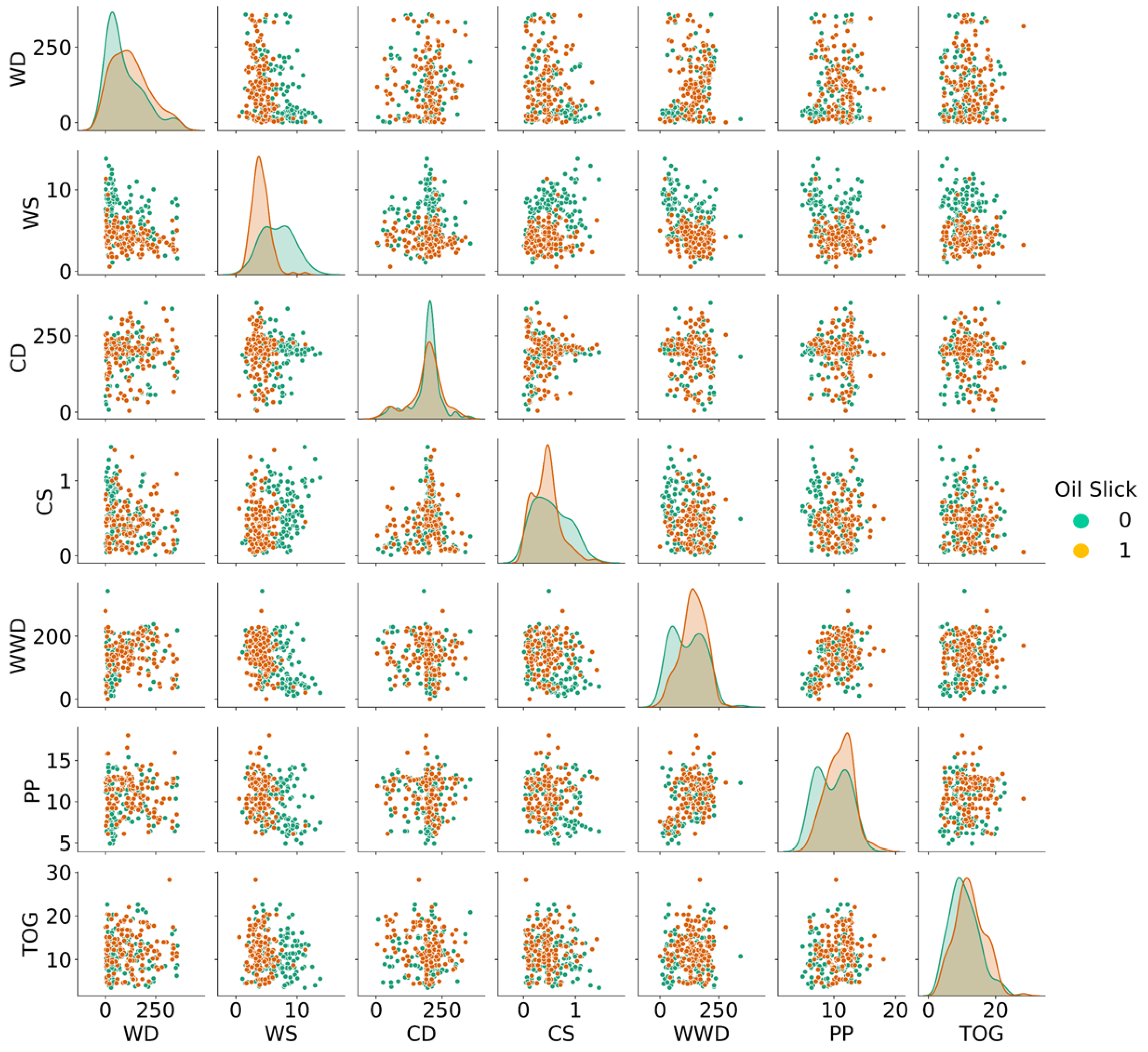
Figure 2.
Flowchart of the methodology proposed in this paper.
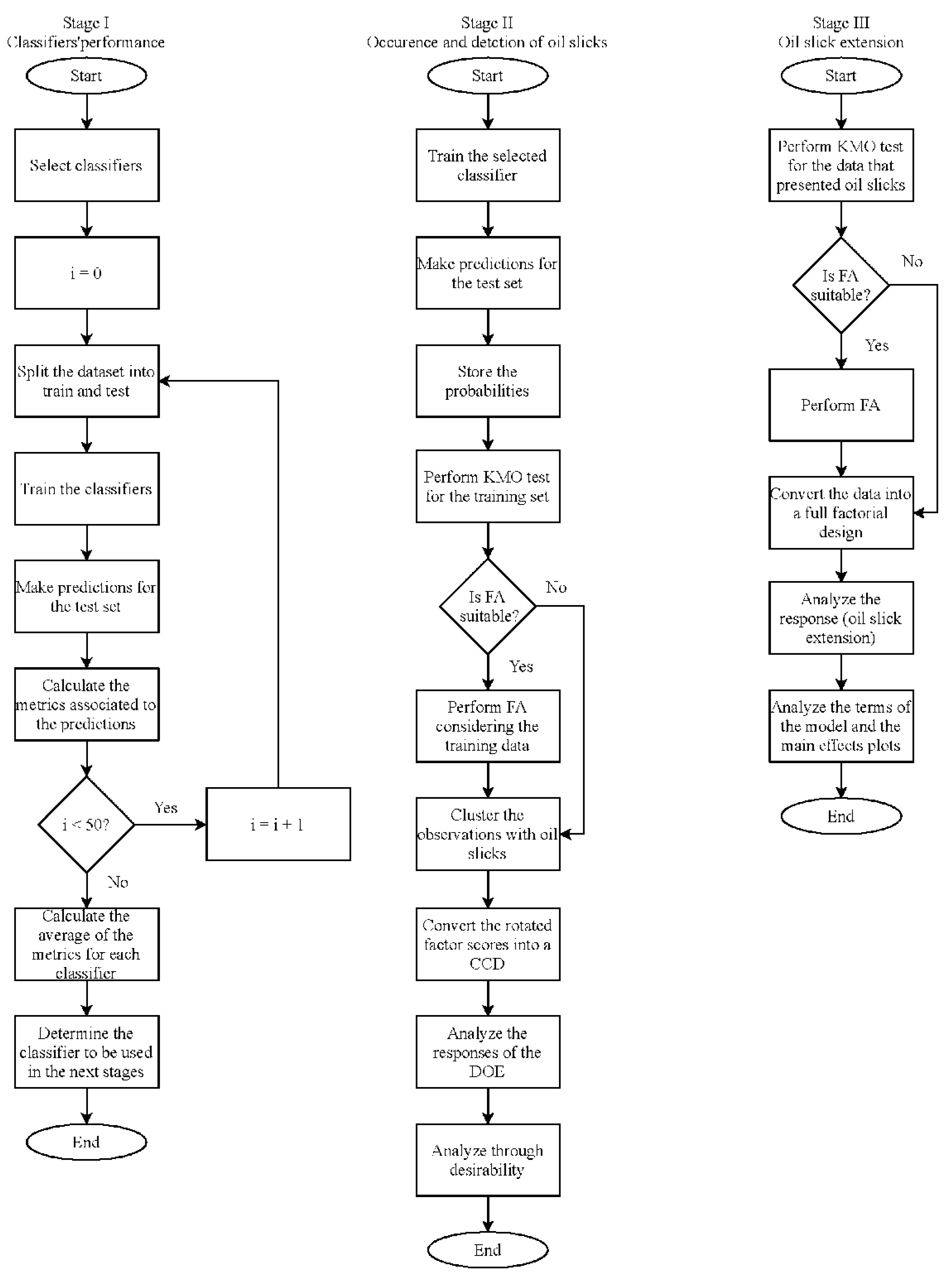
Figure 3.
Feature importance plot for 50 random forest models.
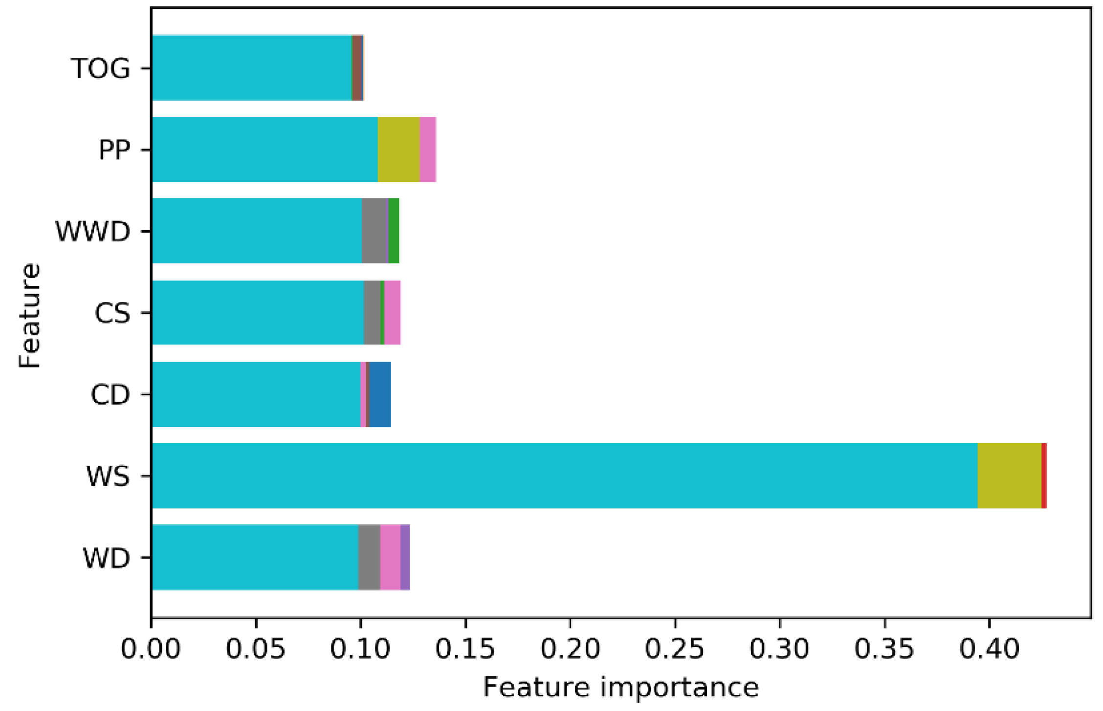
Figure 4.
Feature importance plot for random forest model.
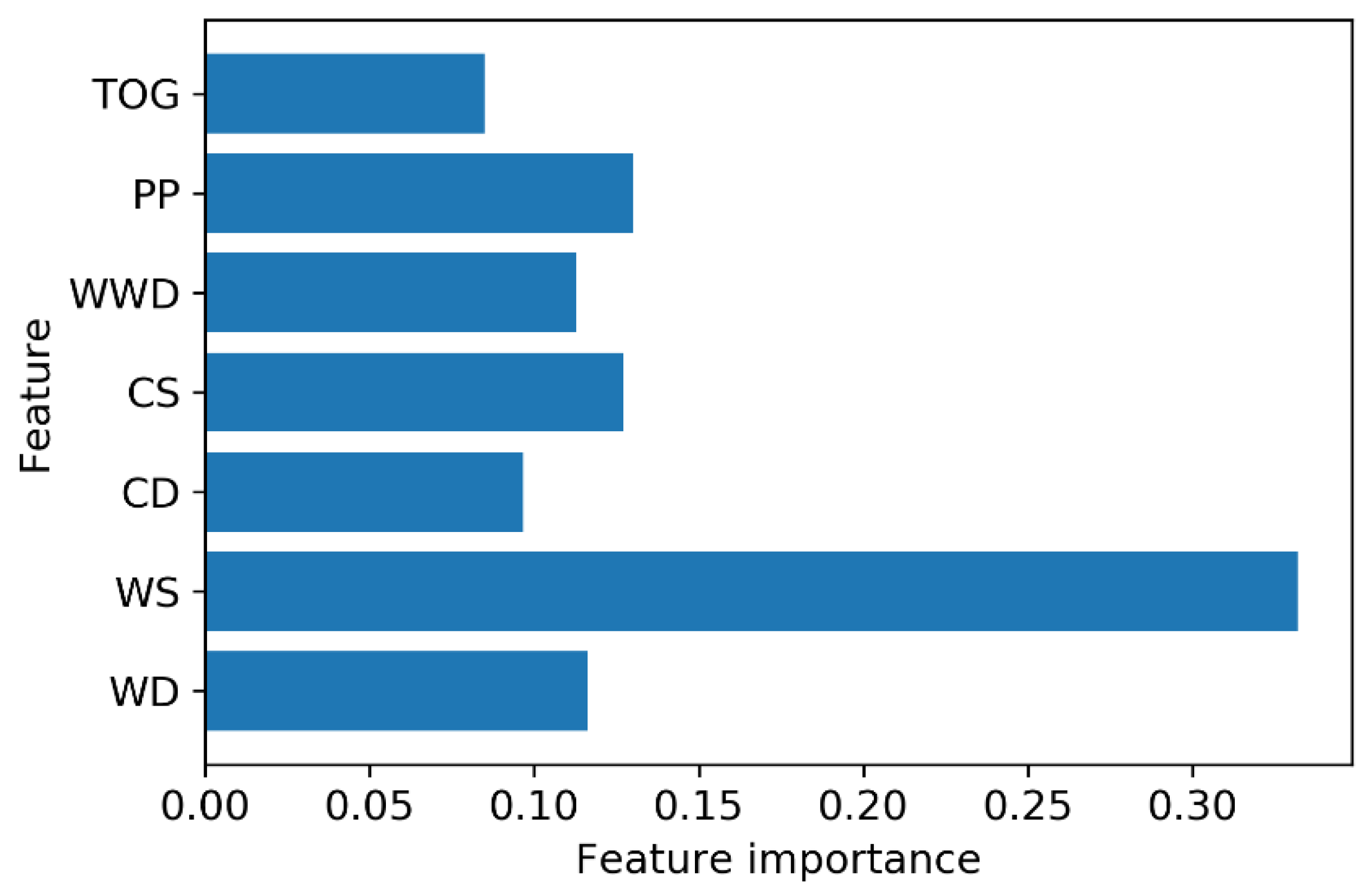
Figure 5.
ROC curve for random forest model.
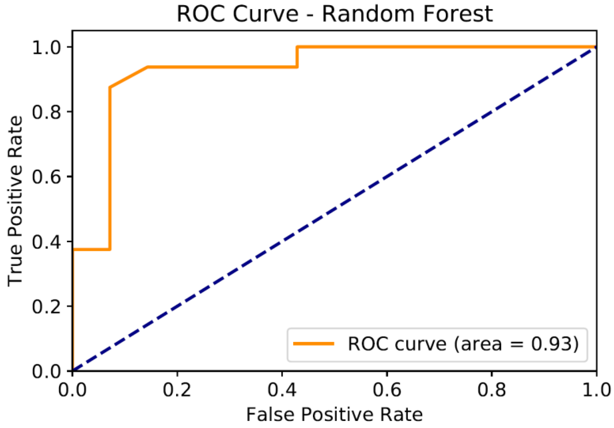
Figure 6.
a) Correlation plot; (b) Correlation plot with p-value < 0.05 boxed.
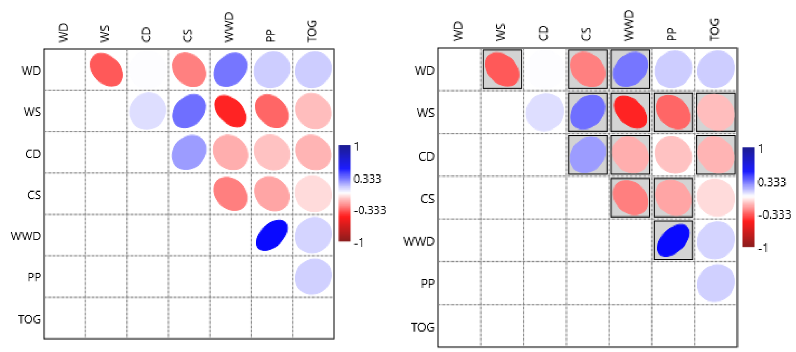
Figure 7.
Desirability results varying one factor at a time.
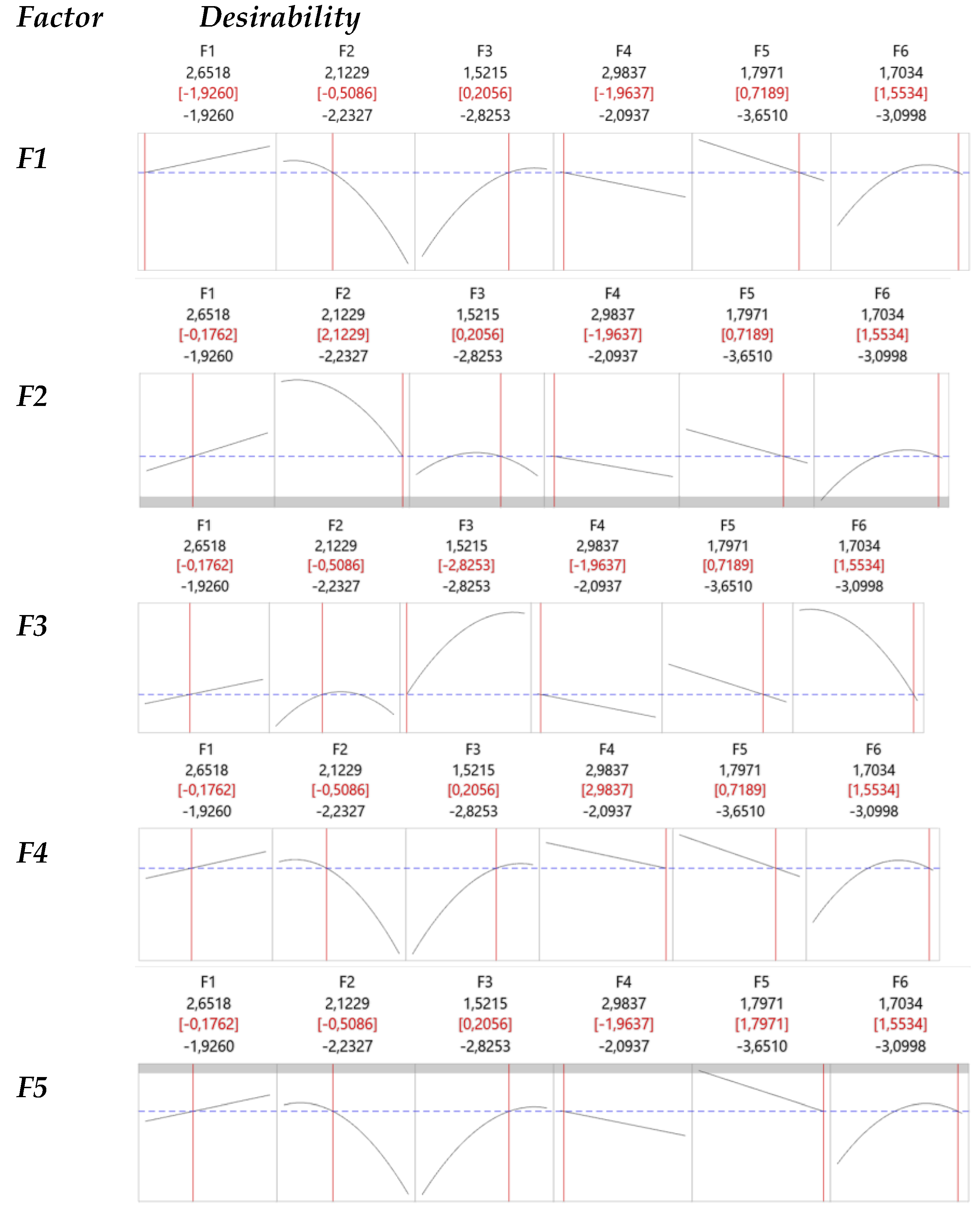
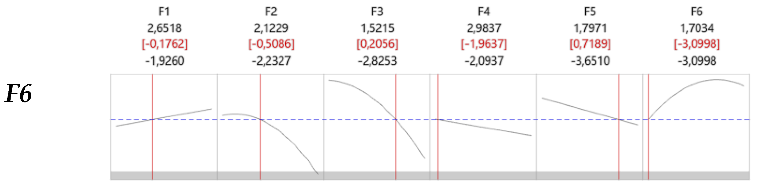
Figure 8.
Contour and surface plots for the occurrence and detection probability model.
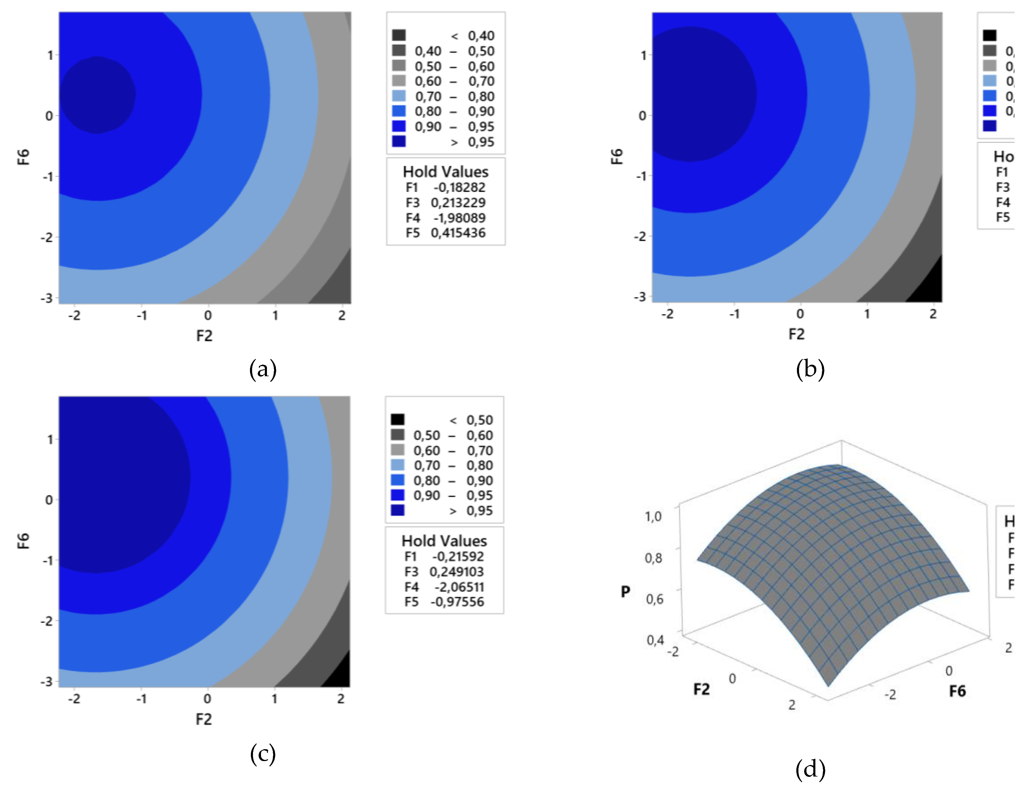
Figure 9.
Main effects plot for the oil film extension.
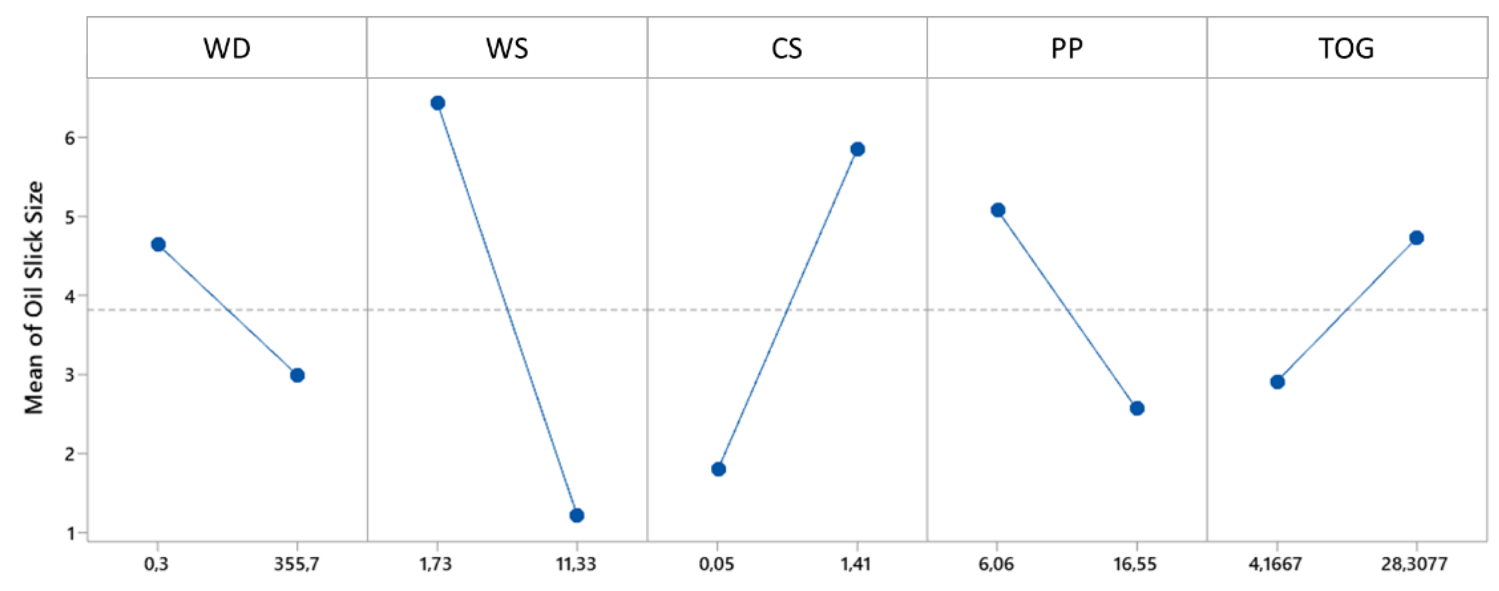

Table 1.
Parametrization and precision metrics for the methods.
| Machine learning algorithm | Parameterization | Acc | Sp | Sn |
|---|---|---|---|---|
| RF | Estimators = 150 Max features = 3 |
0.77 | 0.73 | 0.82 |
| KNN | k = 5 | 0.74 | 0.65 | 0.84 |
| MLP | Number of hidden layers = 2 Number of units = 4 Activation function = Relu Solver = LBFGS α = 0.05 Learning rate = invscaling |
0.71 | 0.68 | 0.76 |
| BLR | Link function = logit | 0.74 | 0.70 | 0.80 |
| SVM | Kernel = RBF γ = 0.1 C = 1 |
0.75 | 0.65 | 0.85 |
Table 2.
Confusion matrix for the Random Forest model.
| Prediction | |||
| Class 0 | Class 1 | ||
| Actual | Class 0 | 12 | 2 |
| Class 1 | 1 | 15 | |
Table 3.
Correlation matrix.
| WS | CD | CS | WWD | PP | TOG | |
|---|---|---|---|---|---|---|
| WD | -0.325 0.000 |
0.003 0.957 |
-0.247 0.000 |
0.267 0.000 |
0.098 0.109 |
0.097 0.110 |
| WS | 0.063 0.302 |
0.281 0.000 |
-0.430 0.000 |
-0.298 0.000 |
-0.128 0.035 |
|
| CD | 0.193 0.001 |
-0.158 0.009 |
-0.119 0.050 |
-0.146 0.016 |
||
| CS | -0.251 0.000 |
-0.176 0.004 |
0.070 0.252 |
|||
| WWD | 0.482 0.000 |
0.083 0.176 |
||||
| PP | 0.092 0.132 |
Table 4.
Factor loadings and communalities obtained through factor analysis.
| Variable | F1 | F2 | F3 | F4 | F5 | F6 | Communality |
| PP | 0.924 | -0.036 | 0.04 | 0 | -0.073 | 0.09 | 0.87 |
| WWD | 0.719 | -0.359 | -0.228 | 0.147 | 0.026 | 0.061 | 0.724 |
| WS | -0.204 | 0.941 | 0.14 | -0.004 | 0.068 | -0.133 | 0.969 |
| WD | 0.079 | -0.14 | -0.971 | -0.02 | -0.049 | 0.116 | 0.985 |
| CD | -0.078 | 0.013 | -0.018 | -0.985 | 0.075 | -0.093 | 0.992 |
| TOG | 0.044 | -0.057 | -0.046 | 0.073 | -0.991 | 0.021 | 0.996 |
| CS | -0.113 | 0.127 | 0.117 | -0.098 | 0.022 | -0.972 | 0.998 |
| Var. | 1.4393 | 1.0542 | 1.0322 | 1.0081 | 1.0019 | 0.9973 | 6.5329 |
| % Var. | 0.206 | 0.151 | 0.147 | 0.144 | 0.143 | 0.142 | 0.933 |
Table 5.
Coefficients for the oil film size model.
| Term | Effect | Coeff | SE Coeff | T-Value | P-Value | VIF |
|---|---|---|---|---|---|---|
| Constant | 3,818 | 0,103 | 37,24 | 0,000 | ||
| WD | -1,655 | -0,827 | 0,107 | -7,72 | 0,000 | 1,57 |
| WS | -5,234 | -2,617 | 0,186 | -14,04 | 0,000 | 1,79 |
| CS | 4,066 | 2,033 | 0,156 | 13,06 | 0,000 | 1,61 |
| PP | -2,522 | -1,261 | 0,139 | -9,05 | 0,000 | 1,89 |
| TOG | 1,823 | 0,912 | 0,13 | 7,03 | 0,000 | 3,16 |
Disclaimer/Publisher’s Note: The statements, opinions and data contained in all publications are solely those of the individual author(s) and contributor(s) and not of MDPI and/or the editor(s). MDPI and/or the editor(s) disclaim responsibility for any injury to people or property resulting from any ideas, methods, instructions or products referred to in the content. |
© 2025 by the authors. Licensee MDPI, Basel, Switzerland. This article is an open access article distributed under the terms and conditions of the Creative Commons Attribution (CC BY) license (http://creativecommons.org/licenses/by/4.0/).
Copyright: This open access article is published under a Creative Commons CC BY 4.0 license, which permit the free download, distribution, and reuse, provided that the author and preprint are cited in any reuse.


