Preprint
Article

This version is not peer-reviewed.

Climate Change and Economic Conditions of Fifty (50) US States: The “Effect Modifier” of Interest Rate in a Semi-Parametric Smooth Varying-Coefficient

Submitted:

10 February 2025

Posted:

13 February 2025

You are already at the latest version

Abstract

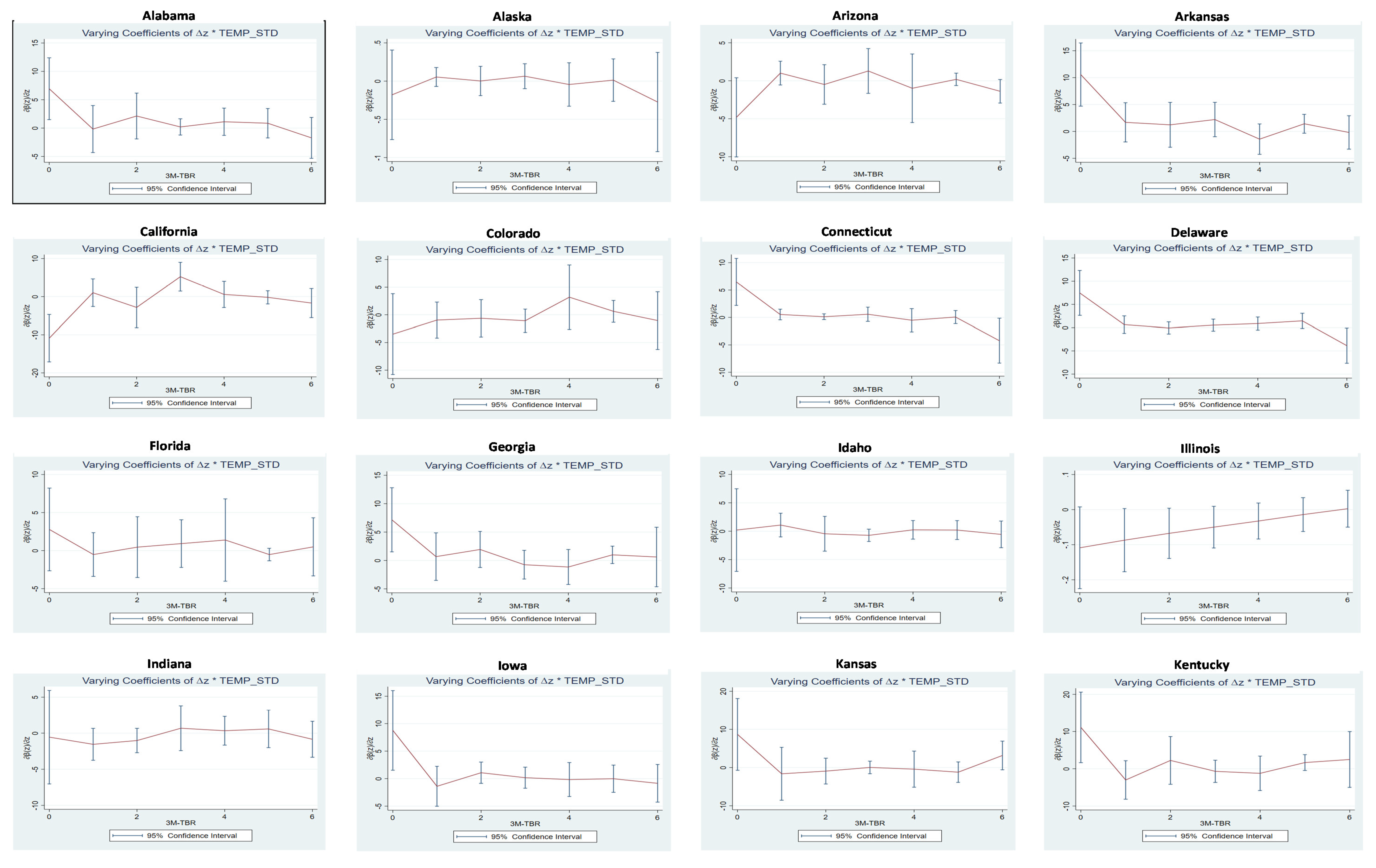
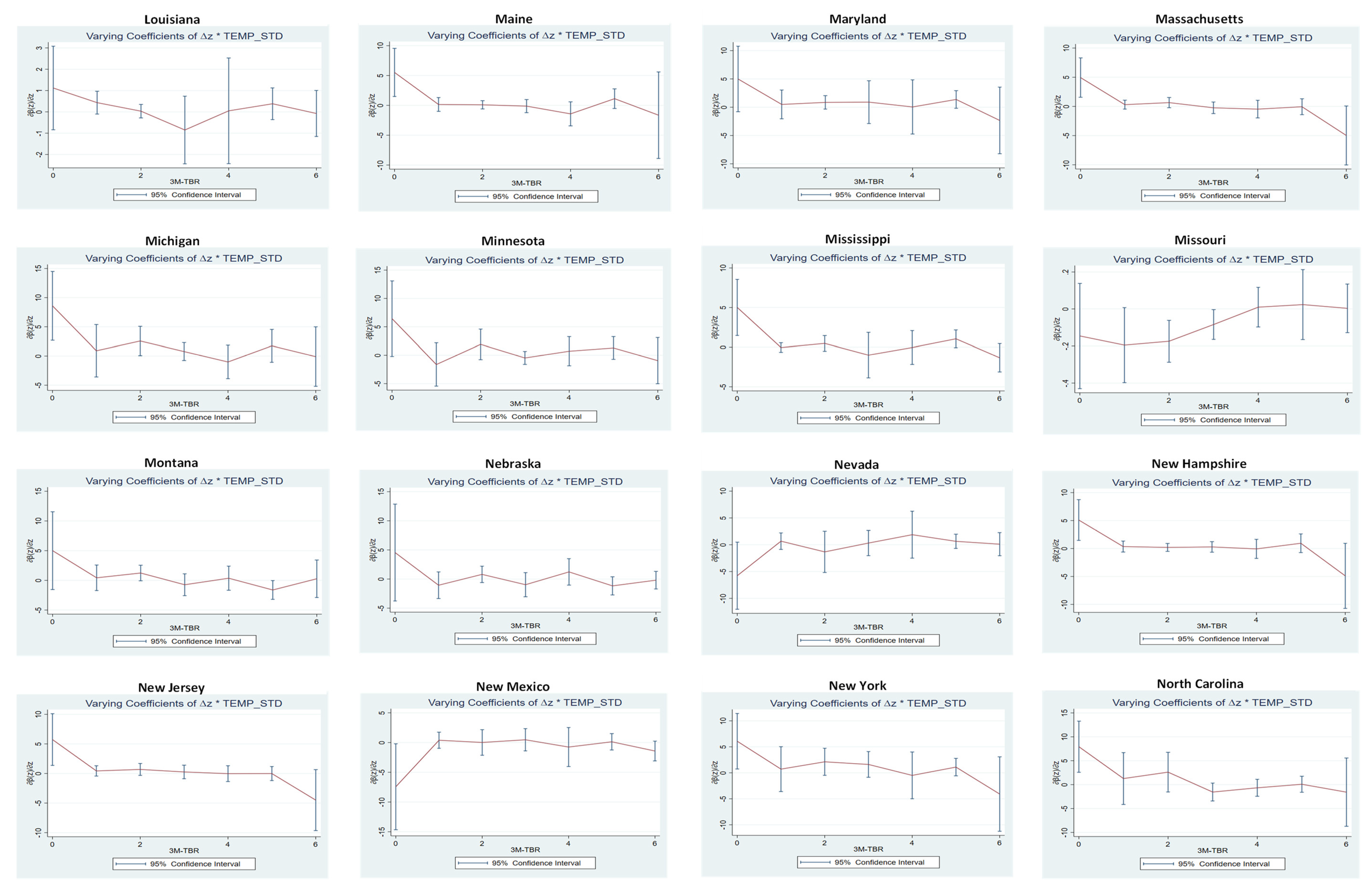
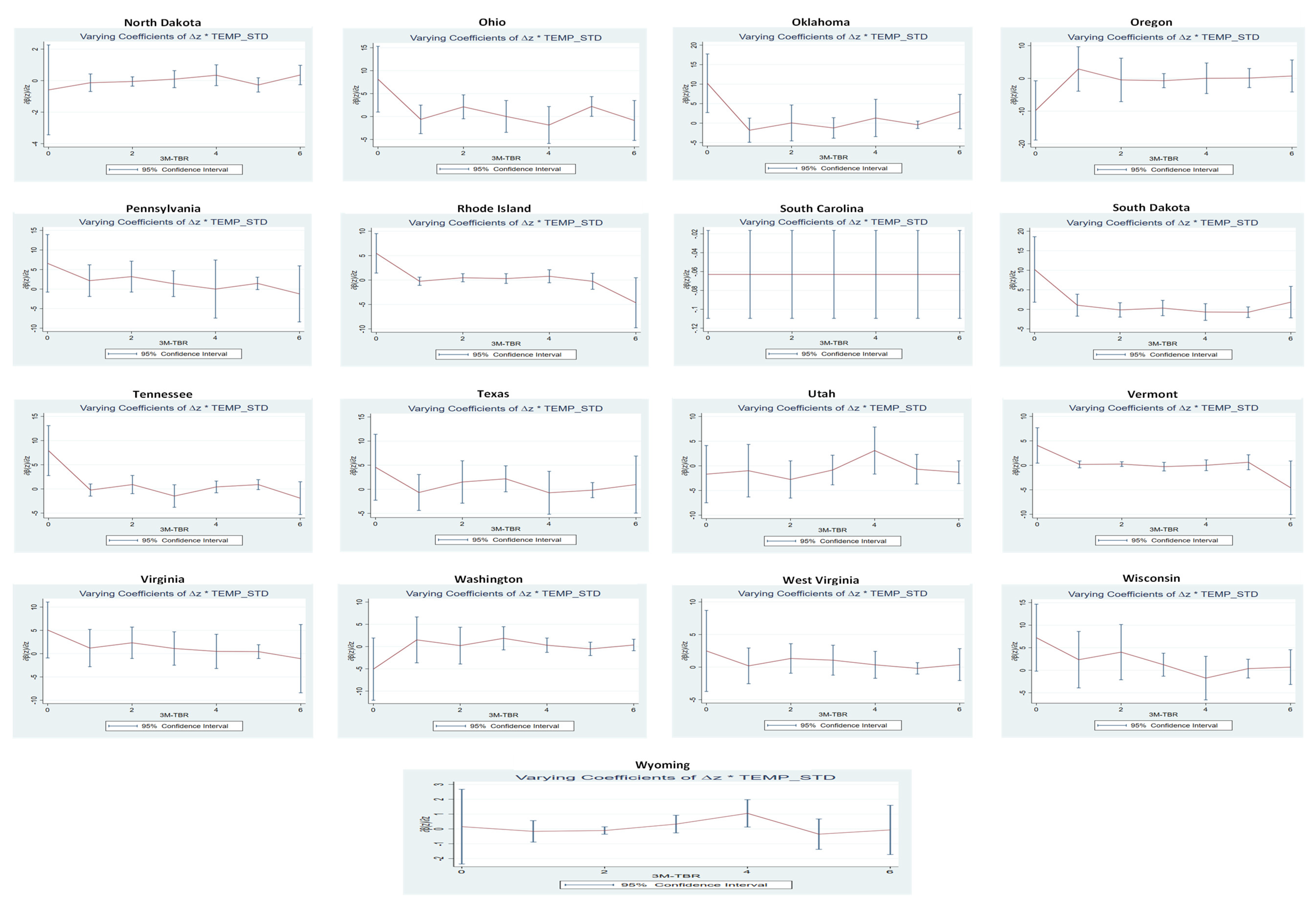
We utilize monthly state-level data from 50 U.S. states to provide the first evidence regarding the role of interest rates as effect modifiers in the commonly held assumption that climate change adversely affects economic conditions. Employing a semi-parametric smooth varying coefficient model (SVCM), we analyze the economic impact of climate change while allowing the coefficient related to economic conditions to vary smoothly with the interest rate (the effect modifier) from April 1987 to December 2022. Our findings indicate that the widely accepted belief in a negative impact from climate change is particularly evident in the coldest states in the U.S. Additionally, we observe that this negative effect manifests as a slower rate of improvement in economic conditions in some of the ten hottest states. We confirm that the effect modifier plays a significant role in about 80% of the states studied. While most states experienced a negative effect of climate change prior to the Global Financial Crisis (GFC), the results largely reverse in its aftermath. From a policy perspective, our validation of heterogeneity in the relationship between climate change and state-level economic conditions suggests that for a geographically diverse economy like the U.S., targeted initiatives tailored to mitigate the economic effects of climate change in specific states are the most effective approach.

Keywords: 
;  ;  ;  ;  

1. Introduction

The phenomenon “climate change” has emerged as a highly debated issue in the 21st century, often resulting in altered precipitation patterns, rising sea levels, storms, wildfires, and heat waves. However, the implications of climate change extend beyond these physical effects, making the economic impact a critical area of focus. Numerous studies have sought to validate the assumption that climate change negatively influences economic activity (see Dell et al., 2014; Burke et al., 2015; Acevedo et al., 2020; Kalkuhla & Wenz, 2020; Adom & Amoani, 2021; Faccia et al., 2021; Donadelli et al., 2021, 2022; Adediran et al., 2023). While most of this research has concentrated on extreme temperatures at the national level, it is vital to examine the economic repercussions of climate change at the state level, particularly in a country with federal states. Our study aims to explore the validity of the hypothesis regarding the adverse effects of climate change under varying economic conditions across different sectors. We investigate the state-level dynamics of the U.S. economy to enhance the existing literature on the relationship between climate change and economic conditions.
When assessing the impact of climate change on economic conditions, it is crucial to avoid oversimplifying data by averaging temperature and precipitation at the country level, particularly in federated states like the U.S. Recent studies, including those by Colacito et al. (2019), Sheng et al. (2022), Cepni et al. (2024), and Mohaddes et al. (2023), have concentrated on understanding the economic effects of climate change on a state-by-state basis. However, our study is distinctive in two significant ways. First, climate change is expected to adversely affect labor productivity (Adom & Amoani, 2021) and exacerbate food prices and food insecurity due to supply chain disruptions triggered by extreme weather events (Faccia et al., 2021). Second, the growth of research and development (R&D) expenditure may also experience negative impacts due to the patent obsolescence channel (Danadelli et al., 2021, 2022). While previous studies have addressed one or two of these avenues, our research adopts a more innovative approach to tackle the issue of information loss. For instance, Sheng et al. (2022) and Mohaddes et al. (2023), in their respective studies, captured the state-level economic activity of the 50 U.S. states in terms of coincident economic activity index (CEAI)1 in the former and as real gross state product (GPS) in the latter (see also, Colacito et al., 2019). Taking a different path in this regard, we instead give preference to a more robust all-encompassing economic condition index (ECI)2 developed by Baumeister et al. (2022).
To the best of our knowledge, the only other paper relevant to our topic is the one by Cepni et al. (2024). However, their study utilizes a panel data structure and a time series approach to filter out national factors based on aggregate climate changes across the U.S. In contrast, our research specifically addresses the dynamic heterogeneity of climate change’s economic impact by examining the distinct economic conditions of all 50 U.S. states. Gaining reliable, evidence-based insights into the state-level effects of climate change is essential for policymakers as they devise targeted initiatives to mitigate its economic repercussions in each state.
It is important to recognize that the primary drivers of economic activity are often shaped at the national level, particularly through policy announcements, and subsequently influence economic conditions at the state level in a trickle-down manner. Our study further distinguishes itself from the reference paper by incorporating a national policy indicator as an “effect modifier” in the relationship between climate change and economic conditions. For example, climate change is expected to impact critical economic variables such as output and inflation, potentially leading to a monetary policy response through adjustments in interest rates. This approach has become a standard practice in monetary policy across the globe.
While interest rates may not have a direct impact on climate change itself, they significantly influence the economic repercussions that arise from it. Key considerations for monetary policy include factors like inflation, economic growth, and employment. Extreme weather events can disrupt these elements, resulting in supply chain interruptions, reduced labor productivity, and increased prices. Consequently, the economic implications of climate change can affect the decisions made by monetary policy authorities. Depending on their objectives—such as mitigating the impact of climate change on labor productivity or controlling inflation—adjustments to interest rates may be necessary. However, whether these adjustments have effectively alleviated the economic consequences of climate change remains uncertain. To investigate this issue, we hypothesize that interest rates can serve as an “effect modifier” within the climate change-economic condition nexus. We employ a semi-parametric smooth varying coefficient model to test this hypothesis, enabling us to analyze how economic conditions fluctuate with changes in the interest rate. This approach is preferred as it allows for greater flexibility in examining the relationships among the variables of interest.
Our hypothesis regarding an effect modifier in the relationship between climate change and economic conditions aligns with that of Salisu et al. (2024). However, unlike the mentioned study, we assess the robustness of this effect modifier across different economic events, specifically during the pre-global financial crisis (pre-GFC) and post-global financial crisis (post-GFC) periods. The global financial crisis of 2007-2008 had a profound impact on monetary policy dynamics, akin to the Great Depression and Recession of the 1930s. The slowdown in economic activity resulted in a significant reduction in interest rates and a negative easing of monetary policy in the U.S. Following the recovery from the GFC, the subsequent economic boom exacerbated climate change and prompted an upward adjustment in interest rates to restore inflation to the target level. Therefore, we hypothesize that interest rates act as an effect modifier in the connection between climate change and economic conditions, with this role being episodic. To test our hypothesis, we have segmented our sample into pre-GFC and post-GFC groups to investigate whether the economic impact of climate change varies during recessionary and booming phases of economic activity.

2. Data and Preliminary Statistics

The state-level monthly climate change data utilized in this study is measured in terms of temperature (TEMP) anomalies and obtained from NOAA’s National Centers for Environmental Information (NCEI).3 With the exception of Hawaii, the temperature data as measured herein is available for each of the 50 U.S. states under consideration. Regarding the indicator for economic conditions, it is based on the Baumeister et al. (2022) economic condition indexes (ECIs) of the 50 U.S. states (see https://sites.google.com/site/cjbaumeister/datasets). The ECIs, as earlier explained, are derived from a mixed-frequency dynamic factor model with weekly, monthly, and quarterly variables that cover multiple dimensions of the aggregate and state economies. However, while the ECIs were originally calculated weekly, we converted them to a monthly average for uniformity of frequency among the variables of interest, given that the highest frequency for which the climate change data is available is monthly. Finally, the three (3) month treasury bill rate (3M-TBR), which proxy for effect modifier in the climate change –economic conditions nexus, is obtained from the Federal Reserve Economic Data (FRED) online database (https://fred.stlouisfed.org/series/TB3MS).
Between April 1987 and December 2022, the summary statistics presented in Table 1 indicate that all individual U.S. states have experienced warmer temperatures compared to the baseline, with Massachusetts being the sole exception, where the mean temperature is negative. However, the varying dynamics of climate change trends are apparent in the degrees of temperature changes observed. For example, New Jersey and Rhode Island rank as the warmest states, with mean temperature increases of +2.06 degrees Celsius and +2.05 degrees Celsius, respectively, followed closely by Delaware (+1.94 degrees Celsius) and Alaska (+1.82 degrees Celsius). In contrast, Alabama, with a mean increase of +0.50 degrees Celsius, and Oklahoma, at +0.57 degrees Celsius, are among the states experiencing the least warming. Furthermore, the overall mean statistic for the economic conditions index remains mostly positive for over 85% of U.S. states, with Alaska, Massachusetts, New York, South Dakota, Washington, and West Virginia being the few exceptions where the economic conditions appear to have remained depressed during the period under review.
Presented in Figure 1 are the historical trends illustrating potential correlations between the state-level economic conditions of each individual U.S. state and their corresponding temperature anomalies. Notably, despite the observable clustering pattern in the climate change indicator, there are intriguing instances of spikes. These spikes can be categorized as positive anomalies, where the trend surpasses the zero-bound line, and negative anomalies, where the trend falls below that line. A closer examination of the figure reveals that the dynamics of these positive and negative spikes in temperature anomalies vary significantly among the 50 U.S. states and across different time periods. This observation supports our hypothesis regarding heterogeneity in the nexus between climate change and economic conditions. Importantly, some states exhibit a trend where economic conditions align with climate change over the period under review. In contrast, states including Arizona, Arkansas, Delaware, Georgia, Louisiana, and Wisconsin show a clear divergence, while other states demonstrate a mixed relationship across various periods. This complexity further reinforces our argument for the heterogeneity and episodic nature of the relationship between climate change and economic conditions. To address the limitations of the conventional graphical analysis thus far, we will proceed in the following section to present a methodological framework aimed at testing the validity of our hypothesis regarding the heterogeneous economic effects of climate change.
One of the key innovations of this study is the introduction of a novel hypothesis regarding the role of US interest rates as an effect modifier in the nexus of climate change and economic conditions. This unique perspective transcends the conventional pictorial analysis of potential co-movements between climate change and the economic conditions across the 50 states of the United States. Consequently, we expand our preliminary analysis to incorporate a covariance correlation analysis involving the modifier indicator (US interest rate) and the target variable (climate change), which may yield exciting new insights. For instance, Table 2 presents compelling evidence of a negative correlation between climate change and the modifier indicator. We observe this correlation to be statistically significant in over 30 of the 50 US states studied, thereby providing preliminary evidence of the interest rate’s potential to moderate the impact of climate change on economic condition.

3. Methodology

One of our methodological objectives is to place less emphasis on the specific functional forms of the variables of interest. Therefore, we employ a parametric type of regression that enables us to assess the economic impact of climate change while allowing the coefficient related to economic conditions to vary smoothly with the value of the 3M-TBR, which serves as the effect modifier. Our preference for parametric models is partly due to their ease of implementation, but it is crucial to recognize that certain variants of these models have limitations. There are three main variants of non-parametric regression: non-parametric, standard semi-parametric, and semi-parametric. The first limitation arises from the increased flexibility of non-parametric models, which can result in the “curse of dimensionality.” The second limitation relates to model selection procedures, which, according to Rios-Avila (2020), can be computationally intensive, especially with large samples. Since these weaknesses primarily affect the first two variants of non-parametric regressions, we consider the semi-parametric method—combining the flexibility of non-parametric models with the structure of standard models (see Hastie & Tabshiran, 1993; Verardi, 2013; Rios-Avila, 2020)—to be the most appropriate approach for this study. Following the procedure outlined by Rios-Avila (2020), the semi-parametric regression used in this research is formulated as follows:
y = f 0 z + f 1 ( z ) x + f 2 ( z ) x + + f n ( z ) x + ε
The term y in equation (1) is our predicted variable in a linear combination of x , where y represents the state-level economic conditions of the U.S. 50 states and x on the other hand denotes climate change, while f 0 z ,   f 1 ( z ) ,   ,   f n ( z ) capture the unknown nonlinear function of a single smoothing variable ( z ). In a more specific term, the variable z measured the U.S. three- month treasury bill rate is the indicator for our proposed effect modifier. Regarding our estimation procedure, we follows Li and Racine (2007, 2010) to employs the local linear kernel weighted regression that requires choosing the kernel function k and bandwidth  h and is carried out in the neighborhood of some point of reference, z 0 . Hence, for any specific point of reference z 0 , the estimable model is as given below.
y = α 0 + β 0 x + α 1 z z 0 + β 1 x * z z 0 + ε
where X = 1 x z z 0 x * z z 0 and the estimation parameters represented as B = α 0 α 1 β 0 β 1 is given by:
B =   X     W z 0 X 1   X     W z 0 y
Also, since W z is a matrix of kernel weights depending on how close an observation is to the point of interest, z 0 , we estimate at every stem for all the possible value of z . Taken cognizant of the fact that the model is sensitive to the choice of bandwidth, h , we use a leave-one-out Cross-validation C V l o o procedure involving a NewtonRaphson-type algorithm by minimizing the following function:
C V l o o h = min h i = 1 N ω z y i y ^ i 2
where ω z is a matrix of kernel weights depending on how close an observation is to the point of interest, z 0 . More importantly, instead of arbitrarily favoring the semi-parametric smooth varying-coefficient model (SVCM) as the most suitable version of non-parametric regressions, we will scientifically test its specification against alternative parametric models of various types:
y = β 1 x 1 + γ z z + ε
y = β 0 x + γ z + β 1 x * z + ε
y = β 0 x + γ z + β 1 x * z + β 2 x * z 2 + ε
y = β 0 x + γ z + β 1 x * z + β 2 x * z 2 + β 3 x * z 3 + ε
Following the specification test developed by Cai et al. (2000), which is based on a wild bootstrap approach as described in Henderson and Parmeter (2015) and Rios-Avila (2020), the test statistic has a construction similar to that of an F-statistic, as outlined below.
F t e s t = S S R p S S R v c / D F v c D F p S S R v c / N D F v c F 2
where S S R p and S S R v c are the sum of squared residuals for the parametric and SVC models, respectively with their corresponding degrees of freedom respectively symbolized as D F p and D F v c . Note that the preferred model (SVCM) is for the alternative hypothesis H 1 and therefore each of the variants of the parametric models in equations (5a) to (5d) is for the null hypothesis H 0 and therefore a rejection of H 0 implies the preference for the SVCM while the reverse is the case for a non-rejection of H 0 .
Table 2 presents the approximate F-statistic from the specification test for each of the federated states in the U.S. Except for Illinois, Minnesota, South Carolina, and West Virginia—where the null hypothesis supporting each variant of the alternative parametric model is evident—we observe a significant rejection of the null hypothesis in over 90% of the states. In other words, we find that the null hypothesis for the alternative variants of the parametric model is significantly rejected in approximately 45 U.S. states. This reinforces the overall accuracy of the SVCM in modeling the relationship between climate change and economic conditions while considering the role of the effect modifier.

4. Main Empirical Results and Discussion of Finding

In contrast to the traditional line graphs illustrated in Figure 1, Figure 2 presents a pictorial representation of the economic impact of climate change, utilizing the SVCM framework established in the preceding section. The results of our regression analysis reinforce the prevailing view that climate change adversely affects economic activity. Specifically, the findings indicate that initial economic conditions in states such as Alaska, California, Missouri, Nevada, New Mexico, North Dakota, Oregon, Utah, and Washington are negatively influenced by temperature anomalies. Our results align with numerous existing studies that have similarly highlighted the detrimental effects of climate change on economic conditions (Burke et al., 2015; Dell et al., 2012, 2014; Bloesch & Gourio, 2015; Colacito et al., 2019; Kalkuhl & Wenz, 2020; Khan et al., 2021; Donadelli et al., 2021; Sheng et al., 2022). Nonetheless, our research also reveals heterogeneity in the relationship between climate change and economic conditions, indicating that the negative impact of climate change is not uniform across most states.4 The regression results indicate that economic conditions in states such as Alabama, Arkansas, Florida, Georgia, and New York, along with 17 other states, respond positively despite the impacts of climate change. A closer examination of the regression figures reveals that these economic conditions remain above the expected zero bound, albeit at a declining rate in most of the previously mentioned states. This suggests that the anticipated negative effects of climate change on economic conditions are not universally observed in approximately 22 U.S. states; rather, these effects manifest as improving economic conditions, albeit at a decreasing pace.
Among the states where the negative impact of climate change on economic conditions is relatively more pronounced, Alaska and North Dakota rank as the coldest states in the U.S. Conversely, Washington, Oregon, and Utah are positioned as the 15th, 16th, and 19th coldest states, respectively. In states where the adverse effects of climate change coincide with improvements in economic conditions at a declining rate, Florida, Georgia, Alabama, Arkansas, and Arizona rank as the first, fifth, seventh, ninth, and tenth hottest states, respectively. This dynamic not only reaffirms the widely held hypothesis regarding the detrimental impact of climate change on economic conditions but also supports our hypothesis regarding the heterogeneous nature of this relationship at the state level.
Figure 2. Full-sample main regression –based on a semi-parametric smooth varying-coefficient approach.
Preprints 148893 g002aPreprints 148893 g002bPreprints 148893 g002c
In addition to validating the heterogeneity of the adverse effects of climate change on economic conditions, this study contributes to the literature by proposing the hypothesis of an effect modifier. Notably, this novel hypothesis holds true for approximately 80% of the 49 U.S. states examined, although at varying intervals or thresholds concerning the rate of changes in the 3M-TBR. For example, our findings indicate that economic conditions are adversely affected in certain states when the rate of change in the 3M-TBR is below 1%. This suggests that a zero interest rate or a stable rate of change can exacerbate climate change. This aligns well with economic intuition, as a stable or zero-level interest rate serves as an incentive for investment, which, in turn, stimulates economic activity. Increased economic activity has been shown to be a fundamental driver of carbon emissions, thereby contributing to climate change. However, the effect modifier begins to manifest in various states when the rate of change in the 3M-TBR reaches 1% or higher. At this 1% threshold, the negative impact of climate change on economic conditions consistently diminishes and eventually fades in states such as Alaska, Missouri, Nevada, New Mexico, North Dakota, Oregon, and Washington. While the effect modifier remains stable in these states, even at rates exceeding 1%, it’s noteworthy that the benefits from the effect modifier start to decline in states like Alaska and Utah when the rate of change in 3M-TBR surpasses 4%.
We also observe the presence of the effect modifier in states where the negative repercussions of climate change on economic conditions are not absolute and instead become less severe as conditions improve at a decreasing rate. In these instances, raising the rate of change in 3M-TBR from 1% to 5% tends to mitigate and ultimately diminish the pattern of improved economic conditions in states such as Alabama, Connecticut, Delaware, Maryland, Massachusetts, and West Virginia, among others. When the rate of change in 3M-TBR exceeds the 5% threshold, there tends to be a loss of gains associated with the effect modifier in certain states. Lastly, we observe numerous instances where the impact of climate change on economic conditions appears to follow an erratic zigzag pattern across various intervals of change in 3M-TBR. The unpredictability of the impact of climate change on economic conditions at different rates of change in 3M-TBR, evident in approximately twenty states, further motivates us to conduct a robustness check on our findings.

4.1. Robustness Check Results

Intuitively, there are several reasons to believe that the relationship between climate change and economic conditions is episodic. A notable example is the 2007–2008 global financial crisis (GFC), which adversely affected economic activity and consequently reduced emissions and the impacts of climate change. Throughout 2008 and 2009, the United States experienced negative economic growth, with unemployment rates more than double those of early 2007. This context, which also led to the implementation of zero interest rates to revitalize the economy, prompts further investigation into whether our earlier validation of 3M-TBR as a modifier of the negative effects of climate change on economic conditions varies between pre-GFC and post-GFC samples. The regression results presented in Figure 3 and Figure 4 illustrate that economic conditions respond differently to climate change in the pre-GFC period compared to the post-GFC period, as well as across varying rates of change in 3M-TBR. The fact that this finding is observed in 39 out of the 49 U.S. states examined supports our hypothesis that the climate change-economic conditions nexus is indeed episodic. The limited instances where the impact of climate change on economic conditions appeared consistent across both the pre-GFC and post-GFC samples occurred in states such as Alabama, Alaska, Connecticut, Delaware, Florida, Idaho, New Hampshire, New Jersey, North Dakota, and Vermont. In these states, it is observed that, regardless of whether the sample is from before or after the GFC, economic conditions respond negatively to climate change. This negative impact only begins to diminish when the effect modifier is present at a 1% rate of change in the 3M-TRB. Notably, this trend is valid for only 20% of the federated states in the U.S. Conversely, regression results depicted in Figure 3 indicate that approximately 80% of the federated states experienced a depressed effect of climate change during the pre-GFC period, while post-GFC findings in Figure 4 suggest a different scenario. Additionally, although the effect modifier—evident as a reduction in the depressed impact of climate change during the pre-GFC period—becomes apparent in most states when there is a 1% rate of change in 3M-TBR, the threshold at which the benefits from this effect modifier begin to decline varies significantly among different states. In the post-GFC context, we observe that at a 1% rate of change in 3M-TBR, the effect modifier plays a role in maintaining the improved economic conditions noted in many states. However, when the rate of change exceeds the threshold of 2% to 3%, many states respond negatively to climate change during this period. This observation, among others, supports our hypothesis regarding the heterogeneity and episodic nature of the connections between climate change and economic conditions.

5. Conclusion

Covering the period from April 1978 to December 2020, this study investigates various plausible methods to rigorously evaluate the widely accepted premise that climate change adversely affects economic conditions. By analyzing monthly temperature anomalies across 49 U.S. states in conjunction with their respective state-level economic condition indexes (ECIs), we aim to test the following hypotheses: (i) we leverage the federated structure of the U.S. economy along with the diverse climatic characteristics of individual states to assess whether the relationship between climate change and economic conditions is heterogeneous; (ii) we introduce and evaluate the novelty of an effect modifier in this relationship by employing a semi-parametric smooth varying coefficient model (SVCM); and finally, we examine whether the connection between climate change and economic conditions is episodic in nature. First, we demonstrate that the widely held hypothesis regarding the negative impact of climate on economic conditions is directly applicable to approximately 10 of the 49 U.S. states examined. However, in about 45% of these states, the negative effect manifests as improvements in economic conditions, albeit at a decreasing rate. We also confirm the heterogeneity of this relationship, particularly regarding the dynamics of cold and hot states. For instance, Alaska and North Dakota, which are ranked as the two coldest states in the U.S., exhibit a more pronounced negative effect of climate change on economic conditions. In contrast, states such as Florida, Georgia, Alabama, Arkansas, and Arizona—among the ten hottest states—experience this negative effect in the form of improving economic conditions at decreasing rates. Secondly, we find that the novelty hypothesis concerning effect modifiers is overwhelmingly supported in about 80% of the 49 states studied, though at varying intervals or thresholds related to changes in the 3M-TBR rate. Lastly, we reveal that most states faced a depressed impact of climate change during the pre-GFC period, while the situation significantly changed in the aftermath of the GFC. We have observed that the effect modifier manifested differently before the Global Financial Crisis (GFC) compared to after, as well as across varying rates of change in the 3M-TBR. This finding, among others, supports the hypotheses explored in this study. While it is undeniable that climate change is a national-level phenomenon, our evidence of significant heterogeneity in the relationship between climate change and economic conditions suggests that, for geographically diverse economies like the U.S., it is more effective to concentrate on specific initiatives tailored to mitigate the economic impacts of climate change within individual states.
1
The CEAI as utilized in the study by Sheng et al. (2022) includes four indicators namely, nonfarm payroll employment, the unemployment rate, average hours worked in manufacturing and wages and salaries.
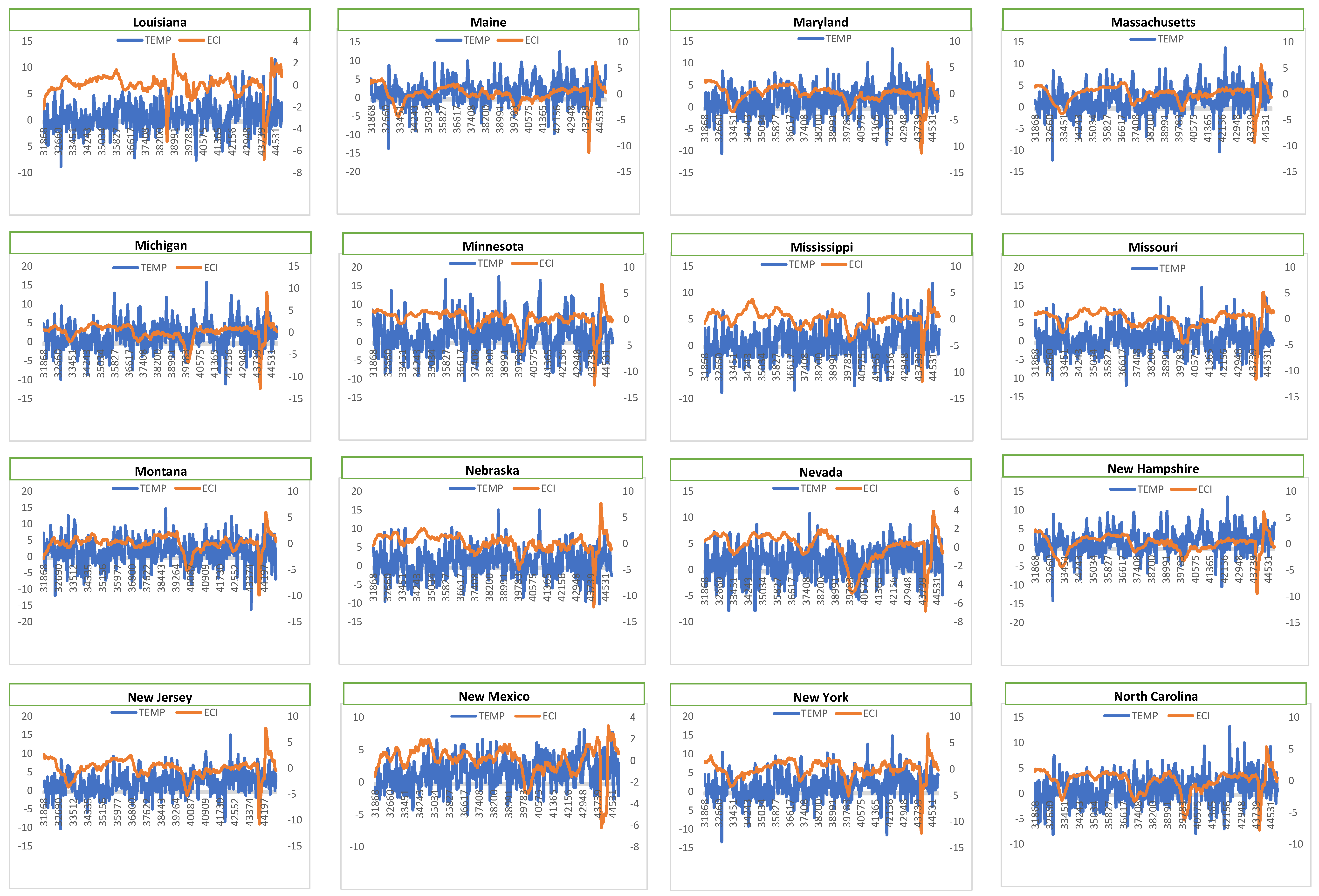
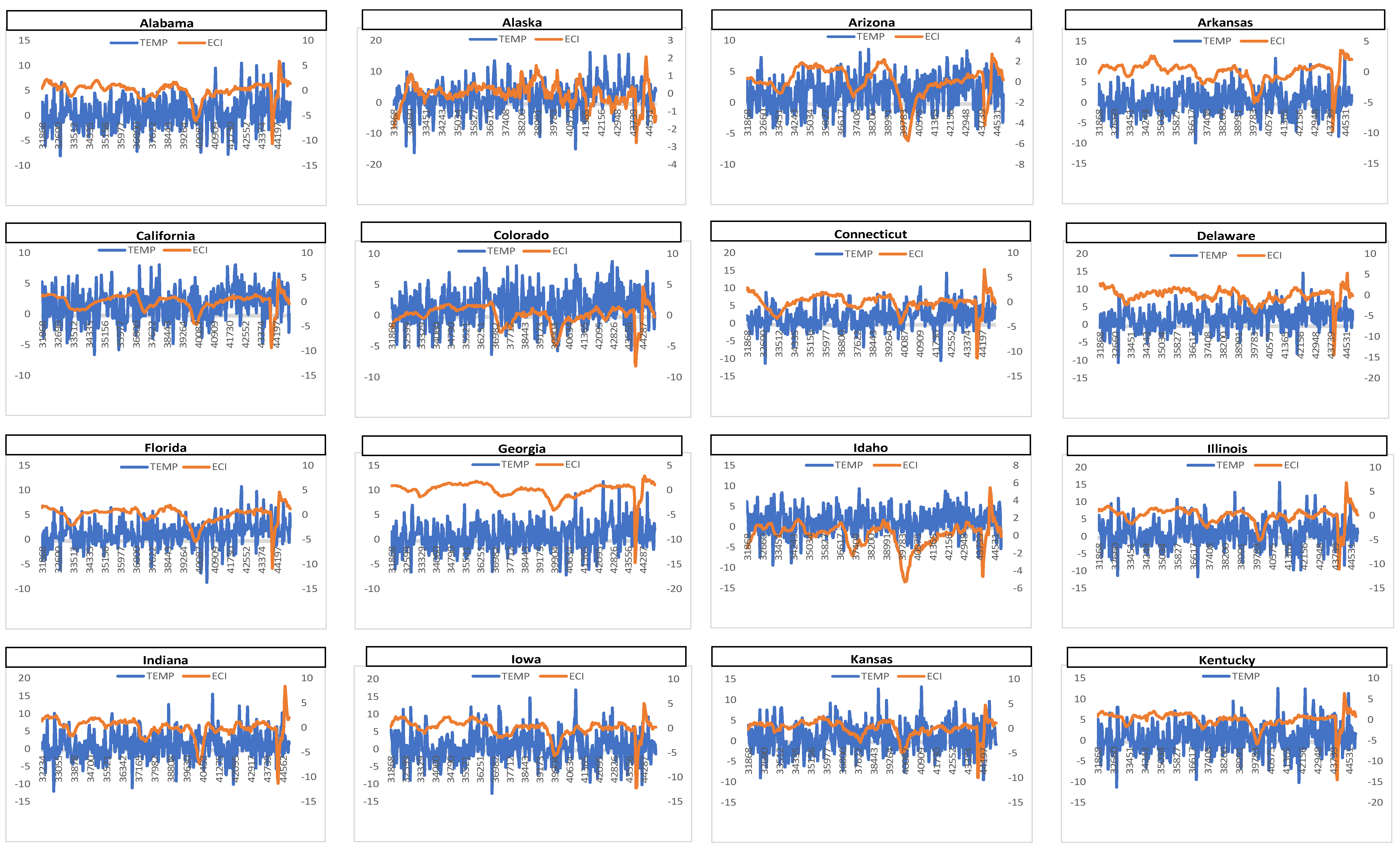
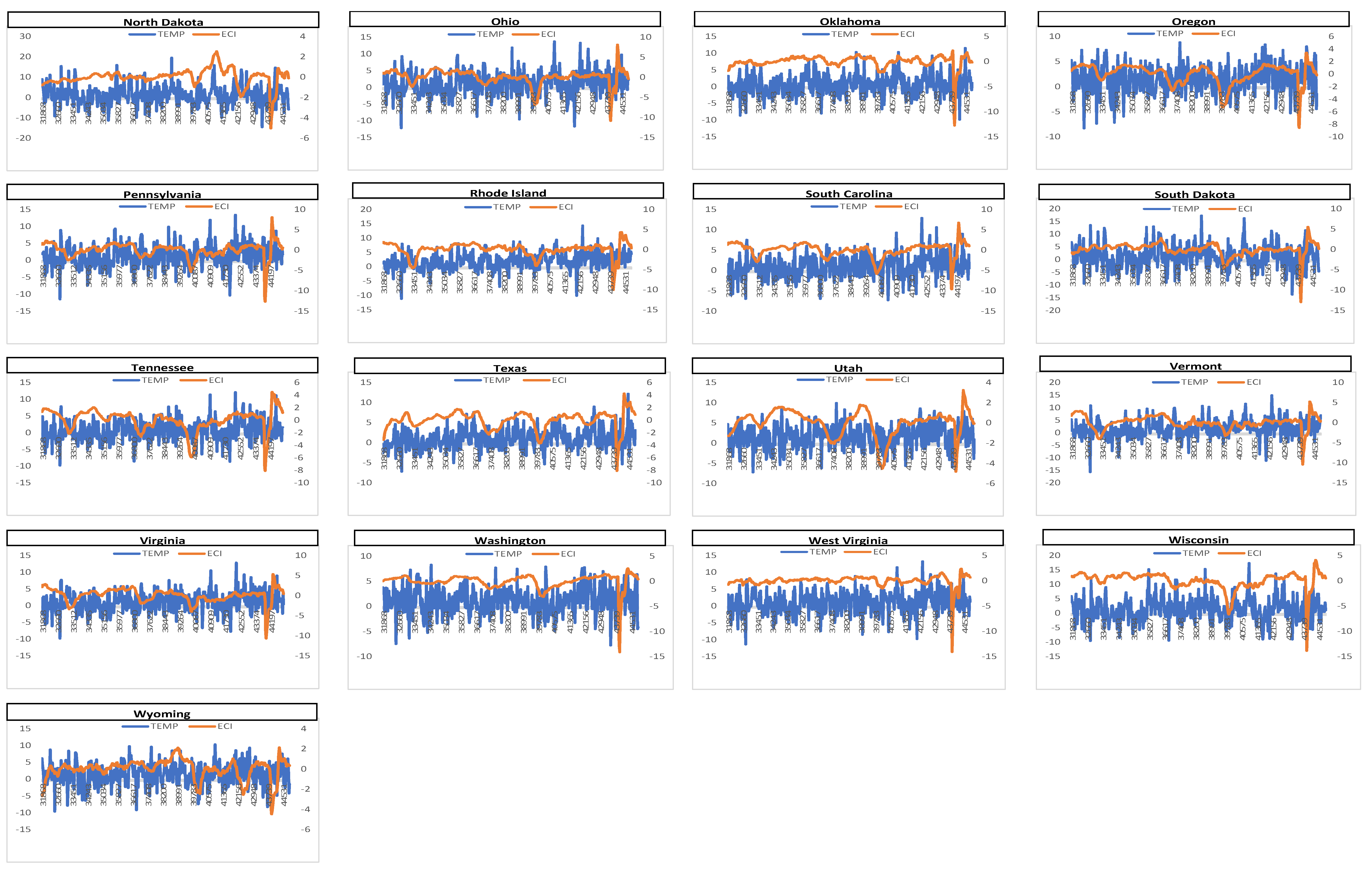
2
The ECI as utilized in this study are based on the work of Baumeister et al. (2022), where the indexes are derived from mixed-frequency dynamic with factor model weekly, monthly, and quarterly variables that covers multiple dimensions of the aggregate and the state economies. In a more specific term, the ECI comprises of variables from six broad dimensions, namely, labour market indicators, mobility measures, real economic activity, financial indicators, household indicators and expectation measures.
3
4
Arizona, Connecticut Delaware, Illinois, Iowa, Maine, Maryland, Massachusetts, Missouri, Montana, New Hampshire, New Jersey, Rhode Island, South Dakota, Texas, Vermont, Verginia, and West Verginia

References

  1. Acevedo, S., Mrkaic, M., Novta, N., Pugacheva, E., & Topalova, P. (2020). The effects of weather shocks on economic activity: What are the channels of impact? Journal of Macroeconomics, 65, 103207. [CrossRef]
  2. Adediran, I.A., Isah, K.O., Ogbonna, A.E., & Badmus, S.K. (2023). A global analysis of the macroeconomic effects of climate change. Asian Economics Letters. [CrossRef]
  3. Adom, P. K., & Amoani, S. (2021). The role of climate adaptation readiness in economic growth and climate change relationship: An analysis of the output/income and productivity/institution channels. Journal of Environmental Management, 293, 112923. [CrossRef]
  4. Baumeister, C., Leiva-León, D., & Sims, E. (2022). Tracking weekly state-level economic conditions. The Review of Economics and Statistics. [CrossRef]
  5. Bloesch, J., and Gourio, F. (2015). The effect of winter weather on U.S. economic activity. Economic Perspectives, 39(1), https://www.chicagofed.org/publications/economic-perspectives/2015/1q-bloesch-gourio.
  6. Burke, M., Hsiang, S.M., & Miguel, E. (2015). Global non-linear effect of temperature on economic production. Nature, 527, 235-239. [CrossRef]
  7. Cepni, O., Gupta, R.., Liao, W., & Ma, J. (2024). Climate Risks and Forecastability of the Weekly State-Level Economic Conditions of the United States. International Review of Finance, 24(1), 154-162. [CrossRef]
  8. Colacito, R., Hoffmann, B., & Phan, T. (2019). Temperature and growth: A panel analysis of the United States. Journal of Money, Credit and Banking, 51, 313–68. [CrossRef]
  9. Dell, M., Jones, B.F., and Olken, B.A. (2012). Temperature shocks and economic growth: Evidence from the last half century. American Economic Journal: Macroeconomics, 4, 66–95.
  10. Dell, M., Jones, B.F., and Olken, B.A. (2014). What do we learn from the weather? The new climate-economy literature. Journal of Economic Literature, 52, 740–98. [CrossRef]
  11. Donadelli, M., Grüning, P., Jüppner, M., Kizys, R. (2021). Global temperature, R&D expenditure, and growth. Energy Economics, 104, 105608. [CrossRef]
  12. Donadelli, M., Jüppner, M., & Vergalli, S. (2022). Temperature variability and the macroeconomy: A world tour. Environmental and Resource Economics, 83, 221-259. [CrossRef]
  13. Hastie, T., and R. J. Tibshirani (1993). Varying-coefficient models (with discussion). Journal of the Royal Statistical Society, Series B55, 757-796.
  14. Kalkuhl, M., & Wenz, L. (2020). The impact of climate conditions on economic production: Evidence from a global panel of regions. Journal of Environmental Economics and Management, 103, 102360. [CrossRef]
  15. Kahn, M.E., Mohaddes, K., Ng, R.N.C., Pesaran, M.H., Raissi, M., & Yang, J.C. (2021). Long-term macroeconomic effects of climate change: A cross-country analysis. Energy Economics, 104, 105-624. [CrossRef]
  16. Li, Q., and J. S. Racine (2007). Nonparametric Econometrics: Theory and Practice. Princeton, NJ: Princeton University Press.
  17. Li, Q., and J. S. Racine (2010). Smooth varying-coefficient estimation and inference for qualitative and quantitative data. Econometric Theory, 26, 1607-1637. [CrossRef]
  18. Mohaddes, K., Ng, R.N.C., Pesaran, M.H., Raissi, M., & Yang, J. (2023). Climate change and economic activity: evidence from US states. Oxford Open Economics, 00, 1–11. [CrossRef]
  19. Rios-Avila, F. (2020). Smooth varying-coefficient models in Stata. Stata Journal, 20, 647-679. [CrossRef]
  20. Salisu, A.A; Isah, K.O, & Vo, X.V. (2024). The “effect modifier” of US interest rate in the economic policy uncertainties and economic conditions of fifty (50) US states: A semi-parametric smooth varying-coefficient approach. The North America Journal of Economics and Finance. [CrossRef]
  21. Sheng, X., Gupta, R., & Cepni, O. (2022). The effects of climate risks on economic activity in a panel of U.S. States: The role of uncertainty. Economic Letter, 213, 110374. [CrossRef]
Figure 1. Historical Trends in Climate Change and Economic Conditions.
Preprints 148893 g001aPreprints 148893 g001bPreprints 148893 g001c
Figure 3. Pre-GFC regression results.
Preprints 148893 g003aPreprints 148893 g003bPreprints 148893 g003c
Figure 4. Post-GFC regression results.
Preprints 148893 g004aPreprints 148893 g004bPreprints 148893 g004c
Table 1. Summary statistics for state-level TEMP and ECIs.
U.S. states Mean U.S. states Mean
TEMP ECIs TEMP ECIs
Alabama 0.501 0.009 Nebraska 1.095 0.182
Alaska 1.820 -0.027 Nevada 1.552 0.067
Arizona 1.667 0.044 New Hampshire 1.720 0.019
Arkansas 0.544 0.022 New Jersey 2.064 0.007
California 1.634 0.025 New Mexico 1.490 0.087
Colorado 1.537 0.067 Ney York 1.533 -0.005
Connecticut 1.853 0.006 North Carolina 1.000 0.003
Delaware 1.937 0.006 North Dakota 1.426 0.000
Florida 1.263 0.054 Ohio 1.233 0.007
Georgia 0.827 0.037 Oklahoma 0.569 0.004
Idaho 1.328 0.056 Oregon 1.426 0.045
Illinois 1.008 0.039 Pennsylvania 1.338 0.018
Indiana 1.036 0.095 Rhode Island 2.058 0.003
Lowa 0.835 0.057 South Carolina 0.936 0.031
Kensas 0.885 0.057 South Dakota 1.207 -0.007
Kentucky 0.790 0.076 Tennessee 0.729 0.037
Louisiana 0.667 0.010 Texas 1.039 0.021
Maine 1.708 0.043 Utah 1.641 0.022
Maryland 1.620 0.050 Vermont 1.702 0.051
Massachusetts -0.027 -0.027 Virginia 1.145 0.068
Michigan 1.614 0.053 Washington 1.170 -0.001
Minnesota 1.603 0.122 West Virginia 1.007 -0.008
Mississippi 0.511 0.084 Wisconsin 1.468 0.023
Missouri 0.719 0.046 Wyoming 1.501 0.017
Montana 1.475 0.036
Note: The mean statistic presented in the table measure the monthly average of the state-level climate change and economic conditions, respectively.
Table 2. Covariance correlation analysis of climate change and the modifiers’ indicator.
U.S. states Correlation result U.S. states Correlation result
Corr. Value Prob. Value Corr. Value Prob. Value
Alabama -0.0719 0.1370 Nebraska -0.0405 0.4019
Alaska -0.1418*** 0.0032 Nevada -0.1446*** 0.0027
Arizona -0.1870*** 0.0001 New Hampshire -0.1382*** 0.0041
Arkansas -0.0506 0.2952 New Jersey -0.1627*** 0.0007
California -0.2107*** 0.0000 New Mexico -0.2396***` 0.0000
Colorado -0.1359*** 0.0048 Ney York -0.0962** 0.0464
Connecticut -0.1346*** 0.0052 North Carolina -0.1203** 0.0126
Delaware -0.1638*** 0.0007 North Dakota 0.0176 0.7147
Florida -0.1100*** 0.0226 Ohio -0.0756 0.1178
Georgia -0.0887* 0.0664 Oklahoma -0.0982** 0.0419
Idaho -0.0809* 0.0940 Oregon -0.1034** 0.0322
Illinois -0.0324 0.5021 Pennsylvania -0.0931* 0.0539
Indiana -0.0555 0.2578 Rhode Island -0.1613*** 0.0008
Lowa -0.0124 0.7973 South Carolina -0.1071** 0.0264
Kensas -0.0669 0.1664 South Dakota 0.0013 0.9783
Kentucky -0.0688 0.1543 Tennessee -0.0808* 0.0945
Louisiana -0.0957** 0.0476 Texas -0.1521*** 0.0016
Maine -0.1425*** 0.0031 Utah -0.1084** 0.0247
Maryland -0.1228** 0.0109 Vermont -0.1253*** 0.0094
Massachusetts -0.1534*** 0.0014 Virginia -0.1129** 0.0198
Michigan -0.0553 0.2526 Washington -0.0656 0.1749
Minnesota -0.0263 0.5860 West Virginia -0.0867* 0.0727
Mississippi -0.0797* 0.0990 Wisconsin -0.0322 0.5050
Missouri -0.0456 0.3452 Wyoming -0.0608 0.2084
Montana -0.0165 0.7325
Note: ***, **, and * implies significant at 1%, 5%, and 10% levels of significance, respectively.
Table 2. Specification Test approximate F-statistic.
H0: Parametric Model
H1: SVCM y=x*b(z)+e
US-50-States Model 1 y=x*b0+g*z+(z*x)b1+e Model 2 y=x*b0+g*z+(z*x)*b1+(z^2*x)*b2+e Model 3 y=x*b0+g*z+(z*x)*b1+(z^2*x)*b2+(z^3*x)*b3+e
Alabama 1.5819***(0.0030) 1.4819**(0.0101) 1.4966***(0.0091)
Alaska 3.0093***(0.0000) 3.2586***(0.0000) 3.1768***(0.0000)
Arizona 2.6096***(0.0000) 1.5063***(0.0087) 1.5379***(0.0066)
Arkansas 1.9885***(0.0000) 1.7897***(0.0002) 1.7967***(0.0002)
California 1.9873***(0.0000) 2.0271***(0.0000) 2.0786***(0.0000)
Colorado 2.1439***(0.0000) 1.7737***(0.0001) 1.7780***(0.0001)
Connecticut 2.5922***(0.0000) 2.2181***(0.0000) 2.2138***(0.0000)
Delaware 2.4421***(0.0000) 2.3910***(0.0000) 2.4859***(0.0000)
Florida 1.8696***(0.0000) 1.7333***(0.0000) 1.7022***(0.0000)
Georgia 1.7968***(0.0000) 1.4433**(0.0134) 1.4626**(0.0115)
Idaho 1.5171***(0.0077) 1.3934**(0.0288) 1.3380**(0.0499)
Illinois 1.1443(0.3351) 0.0932(0.9119) -9.9E+01(1.0000)
Indiana 1.4100**(0.0339) 1.4540**(0.0247) 1.4797**(0.0212)
Lowa 1.7722***(0.0004) 1.7504***(0.0006) 1.7522***(0.0007)
Kensas 1.8918***(0.0000) 1.5975***(0.0013) 1.6256***(0.0010)
Kentucky 1.4107**(0.0139) 1.3436**(0.0307) 1.3722**(0.0233)
Louisiana 2.3123***(0.0000) 2.1134***(0.0002) 2.2333***(0.0001)
Maine 2.1154***(0.0000) 2.1743***(0.0000) 2.1639***(0.0000)
Maryland 1.4473**(0.0171) 1.4750**(0.0138) 1.4907**(0.0126)
Massachusetts 2.7002***(0.0000) 2.4055***(0.0000) 2.3382***(0.0000)
Michigan 1.3753**(0.0326) 1.3719**(0.0352) 1.3795**(0.0342)
Minnesota 1.2169(0.1235) 1.1754(0.1717) 1.1714(0.1790)
Mississippi 2.2464***(0.0000) 1.8481***(0.0023) 1.8635***(0.0025)
Missouri 1.9126*(0.0585) 0.3712(0.8914) 0.5167(0.7129)
Montana 2.7471***(0.0000) 2.2072***(0.0000) 2.0919***(0.0000)
Nebraska 1.3270*(0.0622) 1.3134*(0.0719) 1.2714(0.1018)
Nevada 2.1204***(0.0000) 1.8208***(0.0000) 1.6597***(0.0011)
New Hampshire 2.8003***(0.0000) 2.3229***(0.000) 2.3551***(0.0000)
New Jersey 2.6102***(0.0000) 2.3674***(0.0000) 2.4817***(0.0000)
New Mexico 2.2813***(0.0000) 1.6718***(0.0000) 1.3800**(0.0271)
Ney York 1.9164***(0.0000) 1.8574***(0.0000) 1.8971***(0.0001)
North Carolina 1.8793***(0.0000) 1.8607***(0.0000) 1.8864***(0.0001)
North Dakota 1.6270***(0.0055) 1.5888***(0.0087) 1.6208***(0.0072)
Ohio 1.3876**(0.0256) 1.3866**(0.0270) 1.4207**(0.0201)
Oklahoma 1.3696**(0.0221) 1.1309(0.2156) 1.1283(0.2214)
Oregon 1.5072***(0.0034) 1.4852***(0.0048) 1.4809***(0.0053)
Pennsylvania 1.7013***(0.0005) 1.6699***(0.0008) 1.7036***(0.0006)
Rhode Island 1.9705***(0.0000) 1.9432***(0.0010) 1.9881***(0.0008)
South Carolina 0.0000(0.9999) 0.4675 0.5037
South Dakota 1.8246***(0.0001) 1.4439**(0.0135) 1.4173**(0.0189)
Tennessee 1.9709***(0.0003) 1.9234***(0.0006) 1.9761***(0.0005)
Texas 1.7634***(0.0002) 1.7049***(0.0005) 1.7192***(0.0004)
Utah 1.9701***(0.0000) 1.7720***(0.00001) 1.7582***(0.0001)
Vermont 1.9436***(0.0008) 1.9275***(0.0012) 2.0304***(0.0006)
Virginia 1.4775**(0.0120) 1.3948**(0.0288) 1.4168**(0.0246)
Washington 1.3215**(0.0391) 1.2845*(0.0583) 1.2612*(0.0745)
West Virginia 1.0145(0.4526) 0.7913(0.8908) 0.6752(0.9788)
Wisconsin 1.6000***(0.0011) 1.5378***(0.0029) 1.5374***(0.0030)
Wyoming 4.7800***(0.0000) 3.2818***(0.0000) 3.0360***(0.0000)
Disclaimer/Publisher’s Note: The statements, opinions and data contained in all publications are solely those of the individual author(s) and contributor(s) and not of MDPI and/or the editor(s). MDPI and/or the editor(s) disclaim responsibility for any injury to people or property resulting from any ideas, methods, instructions or products referred to in the content.
Copyright: This open access article is published under a Creative Commons CC BY 4.0 license, which permit the free download, distribution, and reuse, provided that the author and preprint are cited in any reuse.
Prerpints.org logo

Preprints.org is a free preprint server supported by MDPI in Basel, Switzerland.

Subscribe

Disclaimer

Terms of Use

Privacy Policy

Privacy Settings

© 2025 MDPI (Basel, Switzerland) unless otherwise stated