Submitted:
05 February 2025
Posted:
06 February 2025
You are already at the latest version
Abstract
HIV remains a major public health challenge in sub-Saharan Africa, with South Africa bearing the highest burden. KwaZulu-Natal (KZN) has been identified as a hotspot, particularly among females aged 15–34. This study aimed to investigate the spatial distribution and key socio-demographic, behavioural, and economic factors associated with HIV prevalence among females in this age group using a Bayesian spatial logistic regression model. We analysed secondary data from 3324 females who participated in the HIV Incidence Provincial Surveillance System (HIPSS) from June 2014 to July 2015 in uMgungundlovu District, KZN. Bayesian spatial models were fitted using the Integrated Nested Laplace Approximation (INLA) to identify key predictors and spatial clusters of HIV prevalence. Results revealed that age, education, marital status, in-come, alcohol use, condom use, and number of sexual partners significantly influenced HIV prevalence. Higher age groups (20–34 years) had increased odds of HIV infection compared to those aged 15–19. Alcohol use, multiple partners, and STI/TB diagnosis elevated risk, whereas tertiary education and condom use were protective. Two HIV hotspots were identified, with one near Greater Edendale being statistically significant. Findings highlight the need for targeted, context-specific interventions to reduce HIV transmission among young females in KZN.
Keywords:
HIV prevalence
; Bayesian logistic regression
; Kulldorf’s spatial scan statistics
; odds ra-tios
; spatial clustering
1. Background
Human immunodeficiency virus (HIV) remains a significant public health concern in South Africa, home to the largest population of individuals living with HIV globally. KwaZulu-Natal (KZN) is the most affected province, with the highest prevalence rates and profound socio-economic impacts [1]. Women aged 15–34 in KZN are a key demographic in the fight against HIV/AIDS, accounting for a substantial proportion of new infections due to biological vulnerability, societal pressures, and economic challenges [2,3]. Literature documents that women in this age group face heightened risks of HIV transmission, compounded by factors such as inconsistent condom use, early sexual debut, substance abuse, and concurrent sexually transmitted infections (STIs) [4,5]. Poverty, unemployment, transactional sex, and intergenerational relationships further contribute to their vulnerability [6]. In addition, intimate partner violence (IPV) exacerbates the risk by limiting women's ability to negotiate safer sexual practices [7]. Geospatial disparities in HIV prevalence in KZN, particularly in peri-urban and rural areas, highlight barriers such as limited healthcare access and high poverty rates [8]. Spatial epidemiology has identified clusters of high prevalence, underscoring the need for targeted interventions [9].
Bayesian spatial logistic regression offers a robust framework for examining spatial, demographic, and individual-level factors influencing HIV prevalence. This approach incorporates spatial dependencies and heterogeneity, essential for understanding geographic variability in HIV burden across KZN [10]. The application of Bayesian spatial logistic regression has been demonstrated in several contexts. For instance, [11] used Bayesian semi-parametric regression to analyse HIV prevalence among men in Kenya, integrating structured and unstructured spatial effects. Similarly, [12] applied Bayesian spatial modelling to study tuberculosis-HIV co-infection in Ethiopia, uncovering significant geographical heterogeneity. These studies underscore the utility of Bayesian approaches in informing public health interventions through spatially detailed risk analyses.
Structured additive models (SAMs) further enhance Bayesian approaches by accommodating non-linear effects of continuous variables alongside spatial random effects [13,14]. This flexibility allows for integrating individual and area-level risk factors, enabling more accurate spatial estimates and better identification of high-risk clusters [15]. The structured additive approach has proven valuable in addressing spatial autocorrelation while elucidating HIV drivers in regions like KZN, where complex interactions between socio-demographic and geographic factors exist. Spatial models like the Besag-York-Mollié (BYM) model have been widely used in HIV research to analyse structured and unstructured spatial effects, often implemented efficiently using integrated nested Laplace approximation (INLA) [16,17]. Such models have revealed significant geographic disparities in HIV prevalence, aiding in the identification of high-risk clusters and guiding public health interventions [15].
The study aimed to investigate the spatial distribution and key demographic, behavioural, and socio-economic factors associated with HIV prevalence among female youth in KwaZulu-Natal, using a Bayesian spatial logistic regression framework with a structured additive model. To the best of our knowledge, there are few studies integrating advanced Bayesian spatial logistic regression framework to exclusively capture both micro-level (individual risk factors) and macro-level (spatial dependencies) determinants of HIV prevalence targeting female youth in KwaZulu Natal. As a result, this study was the first of its kind.
Youth is often defined as individuals aged 15–24 (United Nations). However, this study adopts a broader definition, encompassing individuals aged 15–34, in alignment with regional demographic trends and epidemiological significance. This age range captures critical life transitions that influence HIV risk, including adolescence, early adulthood, and early middle age, as highlighted by [18]. The expanded age range also reflects the South African context, where young adults up to the age of 34 face significant socioeconomic and health vulnerabilities.
2. Methodology
2.1. Study Area Location
Figure 1A and 1B below depict the location of the study area within uMgungundlovu District and the location of the two sub-districts of KwaZulu-Natal Province, namely: Vulindlela (Western part) and the Greater Edendale (Eastern part), respectively.
2.2. Sources of Data and Study Population
We conducted a secondary analysis of data collected from participants in the HIV Incidence Provincial Surveillance System (HIPSS). Briefly, HIPSS was undertaken from 11 June 2014 to 18 July 2015 in rural Vulindela and the peri-urban Greater Edendale areas in uMgungundlovu District (Figure 1A and B) of KZN, South Africa.
From a total of 600 enumeration areas, 591 enumeration areas with more than 50 households were included in the sample. Of these, 221 enumeration areas were drawn randomly. Within an enumeration area, the households were drawn systematically with a random start. The study staff identified households using the Global Positioning Systems receiver to record the geographic coordinates of each randomly selected household. Only one age-eligible individual per household was randomly selected and enrolled following written informed consent. Questionnaires were administered to obtain household- and individual-level data on demographics, socio-economic status, and health-related information. All enrolled participants provided peripheral blood samples for laboratory measurements for HIV.
In the South African context, using the age group 15–34 as a definition of "youth" aligns with official policy frameworks [18]. This range is designed to account for the extended transitional period many young people experience in South Africa due to socioeconomic factors such as unemployment, prolonged education, and delayed family formation. This age group was chosen to capture both adolescent and young adult populations, reflecting the epidemiological realities of HIV risk in KwaZulu-Natal and aligning with local public health policies. A total of 3324 female participants aged between 15–34 years were involved in our study.
2.3. Study Variables
The dependent variable in this study was “HIV prevalence” which was defined as the ratio of the number of HIV positive participants in an enumeration area to the total number of participants in the same enumeration area. In our analysis, we used unweighted HIV prevalence since we were focused on detecting geographic locations where spatial clustering of HIV prevalence occurs.
HIV status among participants in the study population was categorised as a binary outcome:
The covariates included in the study comprised sociodemographic, behavioural, and biological variables. These included age, level of education, marital status, main income, ever consumed alcohol, ever diagnosed of TB, ever diagnosed of STI, number of sexual partners, condom use, forced first sex, ever pregnant, run out of money, meal cuts, being away from home, duration in the community and access to health facilities. We applied the variance inflation factor (VIF) to check for multicollinearity before fitting the models. All the variance inflation factor values were very small, all less than 1.5, indicating that multicollinearity was not a major issue in the fitted model.
2.4. Spatial Autocorrelation
Spatial analysis was used to identify HIV prevalence clustering and examine the influence of related variables. Enumeration Areas (EAs), with geo-referenced boundaries, were the spatial units linked to HIV prevalence data. Observations that are close in space tend to have similar values and exhibit spatial autocorrelation. Spatial models account for this to distinguish between general trends driven by covariates and spatial random variation [19]. The global Moran’s index and Geary’s C statistic were employed to assess spatial autocorrelation, determining whether HIV prevalence is dispersed, random, or clustered.
2.4.1. Global Moran’s Index Statistic
The Global Moran’s Index measures overall spatial autocorrelation across a study area, indicating the presence, strength, and direction of spatial patterns. Positive autocorrelation occurs when neighboring enumeration areas have similar values, while negative autocorrelation suggests contrasting values. When spatial patterns are random, the index approaches zero [20,21,22,23].
The Moran’s Index is calculated as:
where is the total number of enumeration areas, is the value of the variable at location , is the mean of the variable across all enumeration areas, is the spatial weight between enumeration area and enumeration area and indicates the sum of all spatial weights.
2.4.2. Geary’s C Statistic
Geary’s C evaluates spatial autocorrelation by assessing similarity or dissimilarity between values at neighboring locations. Unlike Moran’s Index, it is sensitive to local variations [24,25]. The formula for Geary’s C is:
where N is the total number of enumeration areas (locations), and are the values of the variable of interest at locations i and j, is the mean of the variable across all locations, is the spatial weight between location i and location j, and is the sum of all . Values of C < 1 indicate positive spatial autocorrelation, C > 1 indicate negative spatial autocorrelation, and C = 1 implies no autocorrelation [26].
While Moran’s Index and Geary’s C identify spatial autocorrelation, they cannot differentiate between hot-spots and cold-spots within clusters. For this, Kulldorff’s spatial scan statistic (SaTScan) can be used. It detects significant spatial clusters of risk factors, identifying areas with higher or lower HIV prevalence in circular windows, enabling hotspot and cold-spot analysis [27].
2.5. Bayesian Logistic Regression Models
Bayesian logistic regression is a powerful method for modelling binary outcomes, such as disease presence, by estimating posterior distributions of regression parameters. This approach integrates prior beliefs with observed data, producing posterior distributions that reflect both sources of information [16,28].
The binary outcome follows a Bernoulli distribution:
Bernoulli (, where is the probability that , linked to the linear predictor by the logistic function:
and
where is the intercept, is the vector of covariates for observation and is the vector of regression coefficients. The likelihood function of N observations is expressed as:
Bayesian spatial logistic regression extends this framework by incorporating spatial dependencies, enabling the analysis of structured and unstructured spatial variability in binary data such as disease prevalence [29].
The model is given by: Bernoulli (,
with the probability linked to the linear predictor :
The linear predictor includes spatial random effects:
where represents the spatial random effects.
2.6. Prior Distributions
In Bayesian analysis, prior distributions represent beliefs about parameters before observing data and are combined with likelihood functions to obtain posterior distributions [16,31,32]. Priors are essential in hierarchical spatial models, especially with small sample sizes or variable data, and help regularize the model [33].
Choosing priors involves balancing prior knowledge and non-informativeness. Informative priors guide inference when prior knowledge is available, while weakly informative or non-informative priors are used when prior knowledge is absent. In this study, non-informative priors were used for regression coefficients and random effects variances due to lack of prior knowledge.
Penalized complexity (PC) priors were applied to the precision parameter of the random effects. These priors balance model simplicity and complexity, avoiding issues like overfitting and computational problems associated with flat priors [34,35]. The PC prior for precision is expressed as:
with
and
where is the precision, is the upper bound for the standard deviation of the random effect, and is the probability that .
2.7. Posterior Distributions and Point Estimates
The posterior distribution contains complete information about parameter estimates, summarized using point estimates and credible intervals. Point estimates include the posterior mean, posterior mode, and posterior median, which are used for inference and prediction.
The posterior mean is the expected value of the parameter under the posterior distribution. It is a common estimate, especially when the posterior is symmetric. For a parameter , it is given by:
The posterior mode also known as the maximum a posteriori (MAP) estimate is the mode of the posterior distribution, i.e., the value of that maximises and is expressed as:
where indicates finding the value of that maximises this posterior probability. The MAP estimate is often used when the posterior is skewed, but it can be sensitive to the choice of the prior.
The posterior median is a robust point estimate that divides the posterior distribution into two equal parts. It is less sensitive to outliers compared to the mean or mode.
Credible intervals provide the range where the parameter likely falls with a given probability. A 95% credible interval means there is a 95% probability that the true parameter lies within the interval:
Unlike frequentist confidence intervals, credible intervals offer direct probabilistic interpretation.
2.8. Bayesian Spatial Logistic Regression Models Applied
Bayesian logistic regression incorporates prior beliefs and spatial dependencies. Below are the applied models.
2.8.1. Unstructured Bayesian Spatial Logistic Regression Model:
This model accounts for heterogeneity by incorporating independent and identically distributed random effects, assuming no spatial dependency [16,36]. It is defined as: Bernoulli (,
with
where denotes the unstructured random effects and .
2.8.2. Structured Bayesian Spatial Logistic Regression Model:
This model incorporates spatial dependence using a structured random field, improving predictions by considering the influence of nearby locations. It is defined as:
where and the conditional autoregressive (CAR) model for assumes:
where indicates the spatially structured random effect at location , represents the number of neighbours of location , is a spatial adjacency matrix and is the precision parameter [13,30,37].
2.9. Model Selection Criteria
After constructing the two Bayesian spatial logistic regression models to capture different spatial structures, we compared their performance. Model selection was based on the following model selection criteria: deviance information criteria (DIC) [38], the effective number of parameters (pD), the mean deviance () and the Watanable-Akaike information criteria (WAIC) [39]. Lower DIC, and WAIC values and a higher pD value suggest a better model fit. Hence the best-fitting model was selected based on the smallest DIC, and WAIC and the highest pD.
2.10. Model Diagnostics
After selecting the best-fitting model, we assessed its adequacy using residual plots and normal Q-Q plots. A well-fitted model should have residuals symmetrically distributed around zero, with no clear pattern or trend and constant variance [40,41,42]. Deviations from normality in the Q-Q plot suggest that residuals do not follow a normal distribution. We also examined spatial autocorrelation in residuals using Moran’s I statistic, Geary’s C statistic, and the variogram plot to verify whether the spatial structure was adequately captured. High spatial autocorrelation in residuals indicates the model failed to fully account for spatial dependencies [43,44]. Significant Moran's I and Geary’s C values suggest poor model fit. Increasing semi variance with distance indicates spatial autocorrelation, suggesting an inadequate model. Flat variogram suggests spatially uncorrelated residuals, indicating a well-fitted model [43,45]. Additionally, posterior density plots were examined for model validity, reliability, and stability. A smooth, unimodal density plot indicates a well-fitting model, while a multimodal plot may suggest model ambiguity or data issues [16].
2.11. Software and Implementation
The Bayesian spatial logistic regression models were implemented using the Integrated Nested Laplace Approximation (INLA) method [14,46] in R (version 4.4.0). The following R packages were used: “INLA”, “sf”, “sp”, “spdep”, and “dplyr” packages. Spatial relationships between enumeration areas were established using a spatial weight matrix, with neighbours identified via Queen’s contiguity. Additionally, Kulldorff’s spatial scan statistics were applied using SaTScan (version 10.1.3).
3. Empirical Results
Summary statistics for the HIV prevalence rates for all the covariates included in the study are depicted in Table 1. While the summary statistics provide an initial indication of associations, the Bayesian model results are prioritized due to their robustness in adjusting for spatial correlations and confounding effects. This approach ensures that our conclusions are based on a more comprehensive analysis of the data.
There were 3324 females who were included in this research and 1576 individuals were HIV positive giving us an overall HIV prevalence of 47.4% (95% CI: 45.7–49.1), (p-value < 0.0001). We noticed that HIV prevalence increased as age increased, and it was 20.4% (95% CI: 16.8–24.5), 37% (95% CI: 34.2–40.0), 54% (95% CI: 50.8–57.1), and 67.5% (95% CI: 64.2–70.8) for age groups 15–19, 20–24, 25–29 and 30–34 respectively, (p-value < 0.0001). Considering education level, individuals with primary education had the highest HIV prevalence of 70.6% (95% CI: 59.7–80.0) followed by those with no schooling with 55.6% (95% CI: 44.1–66.6), (p-value < 0.0001). Participants who had no source of income had the highest HIV prevalence of 50.5% (95% CI: 43.4–57.6), (p-value = 0.169432).
Looking at the marital status covariate, participants who were divorced and those who were separated, but still legally married had the highest HIV prevalence of 100% (95% CI: 15.8–100.0) followed by participants who were single but had been living with someone as a husband/wife before with an HIV prevalence of 63.7% (95% CI: 55.5–71.8). The p-value for the marital status covariate is 0.000181. The HIV prevalence was higher among participants who were once diagnosed with TB, 63% (95% CI: 54.6–70.8) compared to those who were not diagnosed with TB, 46.7% (95% CI: 45.5–48.5), (p-value = 0.000365). Participants who indicated that they were not using condoms as a prevention method had a higher HIV prevalence, 58.1% (95% CI: 47.0–68.7), compared to those who were using condoms, 47.1% (95% CI: 45.4–48.9), (p-value = 0.056253). Classified by number of sexual partners, HIV prevalence increased as the number of partners increased, and it was 45.5% (95% CI: 43.6–47.3) for participants with 1 partner, 51.6% (95% CI: 45.9–57.3) for participants with 2 partners, and 67.5% (95% CI: 60.6–73.8) for participants with 3 partners, (p-value < 0.0001). HIV prevalence for participants who did not consume alcohol was slightly lower, 45.8% (95% CI: 43.9–47.6), compared to those who were consuming alcohol, 58.5% (95% CI: 53.7–63.3), (p-value < 0.0001). Participants who were diagnosed with STIs had a higher HIV prevalence of 63% (95% CI: 56.2–69.4), compared to 46.3% (95% CI: 44.5–48.1) for participants who were not diagnosed with STIs, (p-value < 0.0001). Based on the forced first sex covariate, participants who had forced first sex had the highest HIV prevalence of 54.7% (95% CI: 43.5–65.4), (p-value = 0.246837). Participants who were away from home had a higher HIV prevalence of 50.1% (95% CI: 44.8–55.5), compared to those who were not away from home, (p-value = 0.407053). For the length in community covariate, the highest HIV prevalence of 60% (95% CI: 14.7- 94.7) was recorded for participants who did not respond and the lowest HIV prevalence of 46.7% (95% CI: 44.8–48.7) was observed for those participants who were always in the community, (p-value = 0.447987). The HIV prevalence was higher among participants who accessed health care, 50.5% (95% CI: 47.7–53.4) compared to those who did not respond, 33.3% (95% CI: 4.3–77.7) and those who did not access health care, 45.6% (95% CI: 43.4–47.8), (p-value = 0.018296). Considering run out of money covariate, participants who ran out of money had the highest HIV prevalence of 49.1% (95% CI: 45.2–52.9), (p-value = 0.618173). The HIV prevalence was slightly higher among participants who had meal cuts, 47.7% (95% CI: 43.7–51.8) compared to those who had no meal cuts, 47.5% (95% CI: 45.6–49.4), (p-value = 0.515632). Lastly, participants who once became pregnant had a higher HIV prevalence of 50.4% (95% CI: 48.4–52.3) compared to those who had never became pregnant, 37.4% (95% CI: 33.9–40.9), (p-value < 0.0001).
The HIV prevalence also varied among enumeration areas (ranging between 0–100%). The geographical distribution of HIV prevalence by enumeration areas is shown in Figure 2. This map was created using ArcGIS software with the application of the “tidyverse”, “sf”, and “tmap” packages in R software.
The result for Moran’s index statistic of HIV prevalence was 0,8157 with a p-value < 0.001, indicating a very strong positive spatial autocorrelation in the wards of uMgungundlovu District (Table 2). The positive and statistically significant Moran’s index value supports that there are clusters of high and low HIV prevalence areas within the study region, suggesting a non-random spatial pattern. The positive Moran’s index also suggests that the HIV prevalence in any two spatial neighbouring wards tended to have similar HIV prevalence.
Furthermore, findings from Geary’s C test statistics support the results from Moran’s index statistic as they both reveal consistent evidence of spatial heterogeneity in HIV prevalence within uMgungundlovu District. The summary statistics results for Moran’s index statistic and Geary’s C statistic are displayed in Table 2 below.
As shown in Table 2, both Moran’s I and Geary’s C indicate significant and strong positive spatial autocorrelation in HIV prevalence. These results confirm spatial heterogeneity, suggesting that HIV prevalence is not randomly distributed but influenced by underlying spatial processes or risk factors in uMgungundlovu District. However, while Moran’s I and Geary’s C detect spatial autocorrelation, they do not differentiate hotspots from cold spots. To address this, Kulldorff’s spatial scan statistics were applied, identifying two clusters of HIV prevalence. The spatial distribution of these clusters is visualized in Figure 3.
Cluster 1, a hotspot with a 2.53 km radius, had an HIV prevalence of 48.4%, a relative risk (RR) of 1.22, and a p-value of 0.025, indicating a 22% higher risk inside the cluster compared to outside. This cluster was located around Greater Edendale. Cluster 2, another hotspot with a 2.28 km radius, had an HIV prevalence of 49.6% and an RR of 1.28, meaning the risk was 28% higher within the cluster. This cluster covered Nadi, KwaMbanjwa, Zayeka, KwaMtogotho, KwaNxamalala, and Henley. However, it was not statistically significant (p = 0.467).
To identify factors associated with HIV prevalence, Bayesian spatial logistic regression was applied, considering sociodemographic, behavioural, and biological factors. Most covariates were statistically significant at the 5% level across all three models. Model selection was based on DIC, pD, , and WAIC, as shown in Table 3.
Based on WAIC, DIC, and pD, the structured model emerged as the best model. It has the lower DIC, pD and WAIC values as shown in Table 3 compared to the unstructured model. The structured model strikes the best balance between model fit, complexity, and predictive accuracy, making it the optimal choice. Hence the results of this research are based on the structured model.
Adjusted odds ratios (OR) together with their corresponding 95% credible intervals (CI) for the participants’ characteristics are displayed in Table 4. These values were obtained from the fitted structured Bayesian spatial logistic regression model implemented in INLA.
Most of the covariates included in the study were significant providing insights into the factors associated with HIV prevalence. Covariates levels with 95% credible intervals including 1, were not statistically significant, and as a result, we did not consider them as predictors of HIV prevalence in our study.
The findings revealed that the odds of HIV prevalence for participants in the age groups 20–24, 25–29 and 30–34 were 2.3373 (OR = 2.3373, 95% CI: 1.7914–3.0526), 4.7446 (OR = 4.7446, 95% CI: 3.6111–6.2339) and 9.1981 (OR = 9.1981, 95% CI: 2.8826–12.2926) times higher than that of age group 15–19, respectively.
Considering education, participants with incomplete secondary were 1.4049 (OR = 1.4049, 95% CI: 1.1948–1.6520) times more likely to be HIV infected compared to those with complete secondary. Participants with no schooling were 1.7177 (OR = 1.7177, 95% CI: 1.0650–2.7732) times more likely to be HIV infected compared to participants with complete secondary. Also, participants with primary education were 2.6117 (OR = 2.6117, 95% CI: 1.5968–4.2759) times more likely to be HIV infected compared to participants with complete secondary. Importantly, participants with tertiary education were 0.5337 (OR = 0.5337, 95% CI: 0.3910–0.7276) times less likely to be HIV infected compared to those with complete secondary.
Results based on main income covariate revealed that participants with salary and or wage had a reduced risk of getting infected with HIV (OR = 0.7061, 95% CI: 0.5215–0.9560), compared to those with no source of income.
We found that individuals who were legally married had a reduced risk of getting infected with HIV (OR = 0.3708, 95% CI: 0.1497–0.9185), compared to those who were divorced. The results also revealed that there was a higher likelihood of being infected by HIV among individuals who were diagnosed with TB (OR = 1.7986, 95% CI: 1.2473–2.5935), compared to those who never suffered from TB. We also discovered that there was a higher likelihood of getting HIV infection among participants who were diagnosed with STIs (OR = 1.6938, 95% CI: 1.2448–2.3025), compared to those who were not diagnosed with STIs.
Considering number of sexual partners, there was a higher likelihood of being HIV infected among participants who had 3 or more sexual partners (OR = 1.7647, 95% CI: 1.2751–2.4449), compared to those who had one partner. Results based on alcohol consumption showed that individuals who consumed alcohol had odds of HIV prevalence that was 1.6438 (OR = 1.6438, 95% CI: 1.3100–2.1684) times higher than those who were not consuming alcohol. Lastly, we found that using condoms as a prevention method, reduced the risk of being HIV infected (OR = 0.5516, 95% CI: 0.3482–0.8737), compared to not using condoms.
The results above indicate that age group, education levels, source of income and marital status, along with behaviours like alcohol use, condom use and having multiple sexual partners, are the key predictors of HIV prevalence. Also, being diagnosed with sexually transmitted infections (STIs) and TB increases the chances of getting infected with HIV.
After fitting the model, the smoothed HIV prevalence rates were calculated and are displayed in Figure 4.
Comparing the HIV prevalence intervals in Figure 2 (unsmoothed prevalence rates) and Figure 4 (smoothed prevalence rates), we observe that the intervals differ. However, areas with high HIV prevalence in the unsmoothed data remain high-prevalence areas in the smoothed data, indicating consistency in spatial patterns.
Model performance was assessed using residuals plot and normal Q-Q plot for model adequacy and Moran’s I, Geary’s C statistic, and the variogram plot to evaluate spatial autocorrelation in residuals. Figure 5 below displays the residuals plot.
Figure 5 displays residuals that are symmetrically distributed around zero, showing no clear pattern, and having constant variance. The plot suggests that there is no systematic bias in the model's predictions implying that the model fits the data well. Figure 6 below displays the Q-Q plot of the residuals.
The Q-Q plot in Figure 6 shows an S-shaped pattern, indicating deviation from normality with heavier tails. However, in spatial modelling, residuals are not always expected to be normally distributed due to inherent spatial dependencies. This characteristic is well-documented in spatial statistics [31,37,43,47,48].
The global Moran’s I statistic for residuals was 0.0009971 (p = 0.4549), suggesting no significant spatial autocorrelation. This indicates that the structured model has adequately captured the spatial structure in the data.
Similarly, Geary’s C statistic was 1.0010397 (p = 0.5349), further confirming that residuals are not spatially autocorrelated. Since both Moran’s I and Geary’s C suggest no significant spatial dependence, the model appears to fit well.
Additionally, the variogram plot in Figure 7 provides strong evidence that residuals are spatially uncorrelated, further supporting the model’s adequacy.
The plot shows a flat semi variance around 0.20, indicating no spatial autocorrelation in the residuals. This suggests that the residuals are spatially independent. If spatial dependence were present, the semi variance would increase with distance, which was not observed.
The posterior density plots for statistically significant regression parameters in Figure 8 display smooth curves with single peaks, indicating stability and proper model convergence.
Based on the spatial autocorrelation tests applied, the results revealed that the residuals were not spatially autocorrelated, implying that the structured model was appropriate and had captured the spatial structure in our data. This is also supported by smooth and unimodal plots displayed by the posterior density plots.
4. Discussion
This study employed a Bayesian spatial logistic regression approach to identify the prevalence and risk factors associated with HIV/AIDS among female youth in KwaZulu-Natal, South Africa, using a structured additive model. The findings indicate significant spatial clustering of HIV prevalence, with sociodemographic, behavioural, and biological factors influencing the risk of infection.
The structured additive model revealed significant spatial variations in HIV prevalence, underscoring the influence of geographic location on HIV risk among female youth. These findings align with existing literature highlighting the clustering of HIV infections in areas with limited access to healthcare services, high population densities, and socio-economic disparities [49]. Addressing spatial inequalities requires targeted interventions in high-risk areas, such as rural and peri-urban settings, where female youth may face barriers to accessing sexual and reproductive health services.
The study identified age as a key determinant of HIV prevalence. Participants aged 20–24, 25–29, and 30–34 had significantly higher odds of HIV infection compared to those aged 15–19. This reflects the high burden of HIV among young adult women, often driven by power imbalances in relationships, transactional sex, and limited access to preventive services [8,50,51].
Education emerged as another critical factor. Lower educational attainment was strongly associated with higher HIV prevalence, while tertiary education was protective. These findings highlight the role of education in empowering young women with knowledge about HIV prevention and increasing their ability to make informed decisions about their sexual health [52,53,54]. Socioeconomic factors, such as income source, were also significant. Female youth earning a salary or wage were less likely to be HIV positive, emphasizing the protective role of financial independence and economic empowerment [55,56].
Risky sexual behaviours, including multiple sexual partners and inconsistent condom use, were significant predictors of HIV infection. These findings align with studies showing that such behaviours amplify the risk of HIV transmission in high-prevalence settings [57,58]. Alcohol use was also associated with higher odds of HIV infection, consistent with evidence that alcohol impairs judgment and increases engagement in risky sexual behaviours [59,60,61].
Health factors, including co-infections with TB and STIs, were strongly associated with HIV infection. These co-morbidities exacerbate vulnerability to HIV, emphasizing the need for integrated healthcare approaches addressing HIV and related infections [62,63,64].
Legal marriage and condom use were protective against HIV infection. Condom use remains one of the most effective strategies to prevent HIV transmission [56,65]. The protective effect of marriage may be due to reduced exposure to high-risk sexual networks, although this depends on the stability and fidelity of the marital relationship [66,67].
The identification of two HIV hotspots in the study area around Greater Endendale and areas around Nadi and KwaMbanjwa is crucial for understanding spatial disparities in HIV prevalence. These hotspots highlight the geographic concentration of HIV prevalence, suggesting that local factors such as socio-economic conditions, healthcare access, and behavioural risk factors may contribute to higher transmission rates in specific areas [54,58,61]. Identifying these clusters is vital for targeted public health interventions, such as focused awareness programs, HIV testing, and prevention efforts, particularly in regions with higher risk [63,64]. By understanding the spatial distribution of HIV, resources can be more effectively allocated, ultimately reducing the burden of the epidemic in high-prevalence regions [67].
5. Conclusions
This study highlights the significant spatial variation in HIV prevalence among female youth in KwaZulu-Natal, South Africa, and identifies key demographic, behavioural, and health factors associated with increased risk. The Bayesian spatial logistic regression approach allowed for the integration of spatial effects and covariates, providing a nuanced understanding of HIV risk in this population. Key findings include the high odds of HIV prevalence among young adults aged 20–34, particularly those with lower educational attainment and limited economic opportunities. Risky behaviours, such as alcohol use, multiple sexual partnerships, and inconsistent condom use, further compound the vulnerability of female youth. Additionally, co-infections with TB and STIs significantly increase the likelihood of HIV infection. The protective role of tertiary education, salaried employment, condom use, and legal marriage emphasizes the importance of multi-sectoral approaches to HIV prevention. Strategies should focus on improving education, promoting economic empowerment, increasing access to HIV prevention services, and addressing co-infections in integrated healthcare programs. Given the spatial heterogeneity observed, interventions must be geographically targeted to address localized drivers of HIV prevalence. Future studies should build on these findings by incorporating longitudinal data to assess the causal pathways between socio-demographic factors, spatial effects, and HIV prevalence. By tailoring interventions to the unique needs of female youth in specific locations, policymakers can enhance the effectiveness of HIV prevention efforts and reduce the burden of the epidemic in KwaZulu-Natal.
Author Contributions
Conceptualization, Exaverio Chireshe and Retius Chifurira; Data curation, Exaverio Chireshe; Formal analysis, Exaverio Chireshe; Investigation, Ayesha B.M. Kharsany; Methodology, Exaverio Chireshe, Retius Chifurira, Knowledge Chinhamu and Jesca Batidzirai; Supervision, Retius Chifurira, Knowledge Chinhamu and Jesca Batidzirai; Validation, Retius Chifurira, Knowledge Chinhamu and Jesca Batidzirai; Writing – original draft, Exaverio Chireshe.
Authors’ information
Exaverio is a PhD student at the Department of Statistics, University of KwaZulu-Natal. Retius and Knowledge are professors, and Jesca is a doctor in the Department of Statistics, University of KwaZulu-Natal, South Africa. Ayesha is a senior scientist at Centre for the AIDS Programme Research in South Africa (CAPRISA) and professor at University of KwaZulu-Natal.
Funding
No funding was received for this study.
Availability of data materials
The dataset used in this research is available upon reasonable request, from the corresponding author. However, restrictions apply to these data’s availability and are not publicly available due to maintaining participants’ confidentiality.
Declarations Ethics Approval and Consent to Participate in the Study
The Biomedical Research Ethics Committee at the University of KwaZulu-Natal (Reference BF269/13; date of approval: 13 May 2024), the KwaZulu-Natal Provincial Department of Health (HRKM08/4), and the Associate Director of the Centre for Global Health (CGH) at the U.S. Centres for Disease Control and Prevention (CDC) in Atlanta, USA (CGH 2014-080) reviewed and approved the protocol, informed consent, and data collection forms for the primary HIPSS study. All eligible participants provided written informed consent prior to study enrolment. All procedures were conducted in compliance with relevant guidelines and regulations.
Consent for Publication
Not applicable.
Competing Interests
The authors declare that they have no conflicts of interest to disclose.
Abbreviations
- HIV: Human Immunodeficiency Virus
- KZN: KwaZulu Natal
- HIPSS: HIV Incidence Provincial Surveillance System
- STIs: Sexually Transmitted Infections
- INLA: Integrated Nested Laplace Approximation
- GIS: Geographical Information System
- MCMC: Markov Chain Monte Carlo
- CI: Credible Interval
- OR: Odds Ratios
References
- Kharsany ABM, Karim QA. HIV infection and AIDS in Sub-Saharan Africa: current status, challenges, and opportunities. The Open AIDS Journal. 2016, 10, 34–48. [CrossRef]
- Kharsany ABM, Cawood C, Khanyile D, et al. Community-based HIV prevalence in KwaZulu-Natal, South Africa: results of a cross-sectional household survey. The Lancet HIV 2018, 5, e427–e437. [CrossRef]
- UNAIDS. In danger: UNAIDS global AIDS update 2022. Geneva: Joint United Nations Programme on HIV/AIDS; 2022.
- Jewkes R, Dunkle K, Nduna M, Shai N. Transactional sex and HIV incidence in a cohort of young women in the Stepping Stones trial. J AIDS Clin Res. 2015, 68, 449–456.
- Zuma K, Shisana O, Rehle TM, Simbayi LC, Jooste S, Zungu N, et al. New HIV infections in South Africa: Evidence from the 2012 population-based household survey. AIDS Res Hum Retroviruses. 2016, 32, 121–134.
- Leclerc-Madlala S. Age-disparate and intergenerational sex in southern Africa: the dynamics of hypervulnerability. AIDS 2008, 22, S17–25.
- Dunkle KL, Jewkes RK, Brown HC, Gray GE, McIntryre JA, Harlow SD. Transactional sex among women in Soweto, South Africa: prevalence, risk factors and association with HIV infection. Soc Sci Med. 2016, 62, 181–193. [CrossRef]
- Tomita A, Vandormael A, Bärnighausen T, de Oliveira T, Tanser F. Social determinants of HIV infection clustering in KwaZulu-Natal, South Africa. AIDS Behav. 2017, 21, 2417–2426.
- Tanser F, Bärnighausen T, Cooke GS, Newell ML. Localized spatial clustering of HIV infections in a widely disseminated rural South African epidemic. Int J Epidemiol. 2009, 38, 1008–1016. [CrossRef]
- Lawson AB. Bayesian disease mapping: Hierarchical modeling in spatial epidemiology. 2nd ed. CRC Press; 2013.
- Ngesa O, Mwambi H, Achia T. Bayesian spatial semi-parametric modeling of HIV variation in Kenya. PLoS One. 2014, 9, e103299. [CrossRef]
- Gemechu LL, Debusho LK. Bayesian spatial modelling of tuberculosis-HIV co-infection in Ethiopia. PLoS One 2023, 18, e0283334. [CrossRef]
- Rue H, Held L. Gaussian Markov Random Fields: Theory and Applications. CRC Press; 2005.
- Rue H, Martino S, Chopin N. Approximate Bayesian inference for latent Gaussian models using integrated nested Laplace approximations (INLA). J R Stat Soc B. 2009, 71, 319–392.
- Tomita A, Vandormael A, Cuadros D, Di Minin E, Heikinheimo V, Tanser F, Slotow R. Spatial clustering of HIV prevalence in KwaZulu-Natal, South Africa: applying Bayesian spatial modeling to a hyperendemic epidemic. Int J Health Geogr. 2020, 19, 1–12.
- Gelman A, Carlin JB, Stern HS, Dunson DB, Vehtari A, Rubin DB. Bayesian Data Analysis. 3rd ed. CRC Press; 2013.
- Tanser F, Bärnighausen T, Dobra A, et al. High HIV incidence in a hyperendemic area of South Africa: A 10-year cohort study. AIDS 2021, 35, 35–45.
- Republic of South Africa. National Youth Policy 2020-2023. Pretoria: Department of Women, Youth and Persons with Disabilities; 2020.
- Gómez-Rubio V. Bayesian Inference with INLA. Boca Raton, Florida: Chapman & Hall/CRC; 2020.
- Moran PAP. Notes on continuous stochastic phenomena. Biometrika 1950, 37, 17–23.
- Waller LA, Gotway CA. Applied Spatial Statistics for Public Health Data. John Wiley & Sons: Hoboken, NJ, USA; 2004.
- Hu W, Mengersen K, Tong S. Risk factor analysis and spatiotemporal CART model of cryptosporidiosis in Queensland, Australia. BMC Infect Dis. 2010, 10, 311. [CrossRef]
- Haining R, Li G. Modelling Spatial and Spatial-Temporal Data: A Bayesian Approach. 1st ed. CRC Press; Boca Raton, FL, USA; 2020.
- Cliff AD, Ord JK. Spatial processes: Models & applications. Pion. 1981.
- Anselin L. Local Indicators of Spatial Association—LISA. Geographical Analysis 1995, 27, 93–115. [CrossRef]
- Geary RC. The contiguity ratio and statistical mapping. Incorporated Stat. 1954, 5, 115–145. [CrossRef]
- Kulldorff M. Spatial scan statistics: Models, calculations, and applications. In: Scan Statistics and Applications. Springer; 1999. p. 303–322.
- Hosmer DW, Lemeshow S, Sturdivant RX. Applied logistic regression. 3rd ed. Hoboken: Wiley; 2013.
- McElreath R. Statistical rethinking: A Bayesian course with examples in R and Stan. 2nd ed. Boca Raton: CRC Press; 2020.
- Lawson AB. Bayesian disease mapping: hierarchical models and spatial dependence. 2nd ed. Boca Raton: CRC Press; 2018.
- Banerjee S, Carlin BP, Gelfand AE. Hierarchical Modelling and Analysis for Spatial Data (2nd ed.). CRC Press; 2014.
- Cressie N, Wikle CK. Statistics for Spatio-Temporal Data. John Wiley & Sons; 2011.
- Gelfand AE, Banerjee S. Bayesian Modeling and Analysis of Spatial Data. CRC Press; 2017.
- Simpson D, Rue H, Riebler A, et al. Penalising model component complexity: a principled, practical approach to constructing priors. Stat Sci. 2017, 32, 1–28. [CrossRef]
- Riebler A, Sørbye SH, Simpson D, Rue H. An intuitive Bayesian spatial model for disease mapping that accounts for scaling. Stat Methods Med Res. 2016, 25, 1145–1165. [CrossRef]
- Wakefield J. Disease mapping and spatial regression with count data. Biostatistics. 2007, 8, 158–183. [CrossRef]
- Besag J, York J, Mollié A. Bayesian image restoration, with two applications in spatial statistics. Annals of the Institute of Statistical Mathematics. 1991, 43, 1–20. [CrossRef]
- Spiegelhalter DJ, Best NG, Carlin BP, van der Linde A. Bayesian measures of model complexity and fit. J R Stat Soc B. 2002, 64, 583–639. [CrossRef]
- Watanabe S. Asymptotic equivalence of the bayes cross validation and widely applicable information criterion in singular learning theory. J Mach Learn Res. 2010; 11, 3571–3594.
- Montgomery DC, Peck EA, Vining GG. Introduction to linear regression analysis. 5th ed. Wiley; 2012.
- Kutner MH, Nachtsheim CJ, et al. Applied Linear Regression Models. McGraw-Hill; 2004.
- Draper NR, Smith H. Applied regression analysis. 3rd ed. Hoboken: Wiley; 2004.
- Cressie NAC. Statistics for Spatial Data (Wiley Series in Probability and Statistics). John Wiley & Sons; 1993.
- Dormann CF, McPherson JM, Araújo MB, et al. Methods to account for spatial autocorrelation in the analysis of species distributional data: A review. Ecography. 2007;30, 609–628. [CrossRef]
- Isaaks EH, Srivastava RM. An introduction to applied geostatistics. Oxford: Oxford University Press; 1989. [CrossRef]
- Rue H, Riebler A, Sorbye SH, Illian JB, Simpson DP, Lindgren FK. Bayesian computing with INLA: A review. Annu Rev Stat Appl. 2017, 4, 395–421. [CrossRef]
- Haining R. Spatial Data Analysis: Theory and Practice. Cambridge University Press; 2003.
- Gamerman D, Lopes HF. Markov Chain Monte Carlo: Stochastic Simulation for Bayesian Inference. 2nd ed. Chapman and Hall/CRC Press; 2006.
- Tanser F, de Oliveira T, Maheu-Giroux M, Bärnighausen T. Concentrated HIV subepidemics in generalized epidemic settings. Lancet 2014, 384, 246–256.
- Pettifor A, MacPhail C, Hughes JP, Selin A, Wang J, Gómez-Olivé FX, et al. The effect of a conditional cash transfer on HIV incidence in young women in rural South Africa (HPTN 068): A phase 3, randomised controlled trial. Lancet Glob Health 2018, 4. [CrossRef]
- Govender K, Beckett SE, George G, et al. Factors associated with HIV in younger and older adult men in South Africa: findings from a cross-sectional survey. BMJ Open 2019, 9, e031667. [CrossRef]
- Hargreaves JR, Bonell CP, Boler T, Boccia D, Birdthistle I, Fletcher A, Pronyk PM, Glynn JR. Systematic review exploring time trends in the association between educational attainment and risk of HIV infection in sub-Saharan Africa. AIDS 2008, 22, 403–414.
- Mabaso M, Makola L, Naidoo I, et al. HIV prevalence in South Africa through gender and racial lenses: results from the 2012 population-based national household survey. Int J Equity Health 2019, 18, 167. [CrossRef]
- Worede JB, Mekonnen AG, Aynalem S, Amare NS. Risky sexual behavior among people living with HIV/AIDS in Andabet district, Ethiopia: Using a model of unsafe sexual behavior. Front Public Health 2022, 10, 1039755.
- Mishra V, Assche SBV. HIV infection does not disproportionately affect the poorer in sub-Saharan Africa. AIDS 2007, 21, S17–S28. [CrossRef]
- Ugwu CLJ, Ncayiyana JR. Spatial disparities of HIV prevalence in South Africa: Do sociodemographic, behavioral, and biological factors explain this spatial variability? Front Public Health 2022, 10, 994277.
- Mah TL, Halperin DT. Concurrent sexual partnerships and the HIV epidemics in Africa: Evidence to move forward. AIDS Behav. 2010;14(1):11–16.
- Wondmeneh TG, Wondmeneh RG. Risky sexual behaviour among HIV-infected adults in Sub-Saharan Africa: A systematic review and meta-analysis. Biomed Res Int. 2023, 2023.
- Fisher JC, Bang H, Kapiga SH. The association between HIV infection and alcohol use: A systematic review and meta-analysis of African studies. Sexually Transmitted Diseases 2007, 34, 856–863.
- Duko, B., Ayalew, M.; Ayano, G. The prevalence of alcohol use disorders among people living with HIV/AIDS: a systematic review and meta-analysis. Subst Abuse Treat Prev Policy 14, 52 (2019).
- Shuper PA, Joharchi N, Rehm J. Lower blood alcohol concentration among HIV-positive versus HIV-negative individuals following controlled alcohol administration. Alcohol Clin Exp Res. 2016, 40, 1460–1465.
- World Health Organization. Global tuberculosis report 2021. 2021. Available from: https://www.who.int.
- Pillay K, Gardner M, Gould A, Otiti S, Mullineux J, Bärnighausen T, et al. Long term effect of primary health care training on HIV testing: A quasi-experimental evaluation of the Sexual Health in Practice (SHIP) intervention. PLoS One 2018, 13, e0199891. [CrossRef]
- Moyo F, Mazanderani AH, Murray T, Technau KG, Carmona S, Kufa T, et al. Characterizing viral load burden among HIV-infected women around the time of delivery: findings from four tertiary obstetric units in Gauteng, South Africa. J Acquir Immune Defic Syndr. 2020, 83, 390–396. [CrossRef]
- UNAIDS. Global HIV & AIDS statistics — 2020 fact sheet. 2020. Available from: https://www.unaids.org.
- Mishra V, Bignami-Van Assche S, Greener R, et al. The Effect of HIV on Adult Mortality in Sub-Saharan Africa: A Comparison of Two Approaches. AIDS 2009, 23, 1617–1627.
- Harling G, Morris KA, Manderson L, Perkins JM, Berkman LF. Age and gender differences in social network composition and social support among older rural South Africans: Findings from the HAALSI study. J Gerontol B Psychol Sci Soc Sci. 2020, 75, 148–159. [CrossRef]
Figure 1.
(A) and (B) Location of the study area.
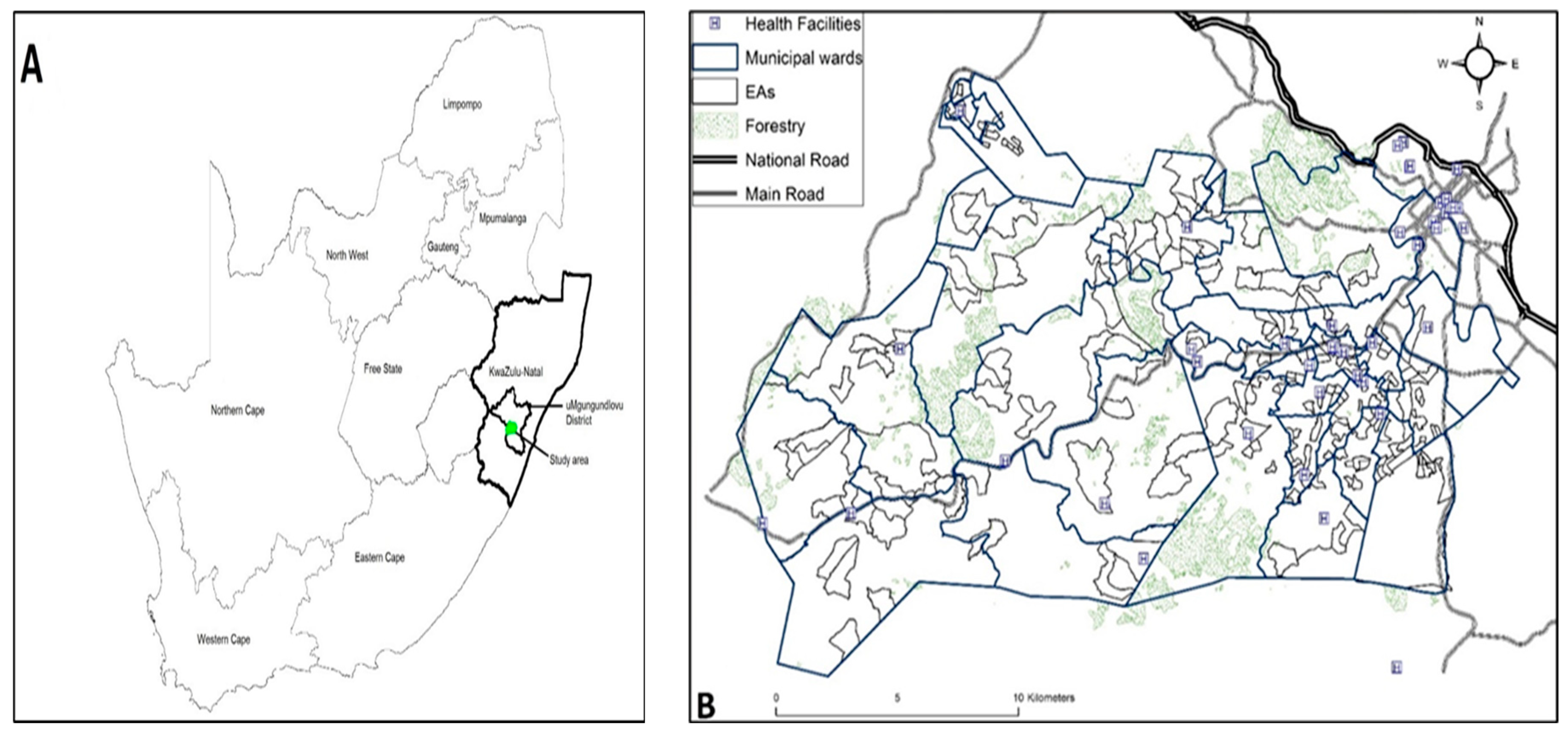
Figure 2.
Geographical Distribution of Unsmoothed HIV Prevalence Among Enumeration Areas.

Figure 3.
Spatial Clustering of HIV Prevalence in uMgungundlovu Municipality.
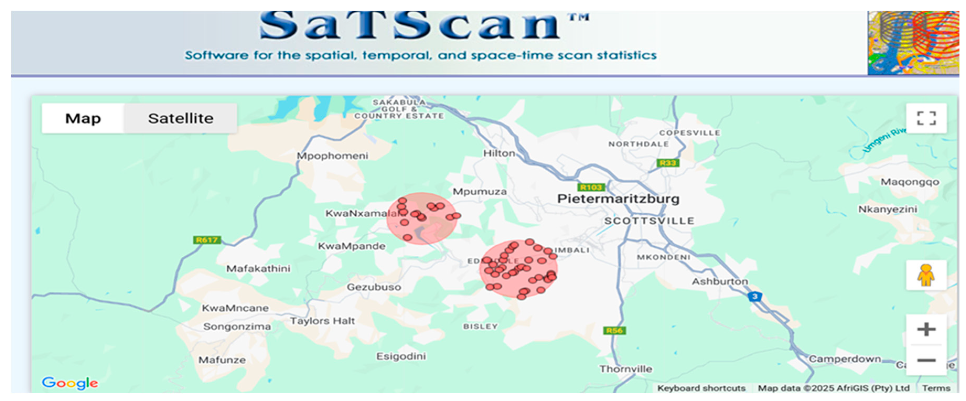
Figure 4.
Geographical Distribution of Smoothed HIV Prevalence Rates.

Figure 5.
Residuals Plot for the Fitted Model.
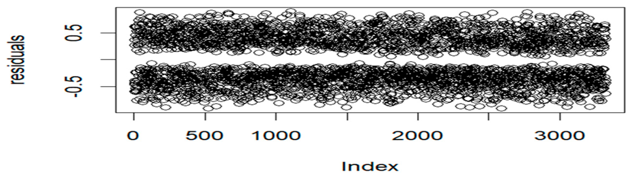
Figure 6.
Normal Q-Q Plot for the Residuals.
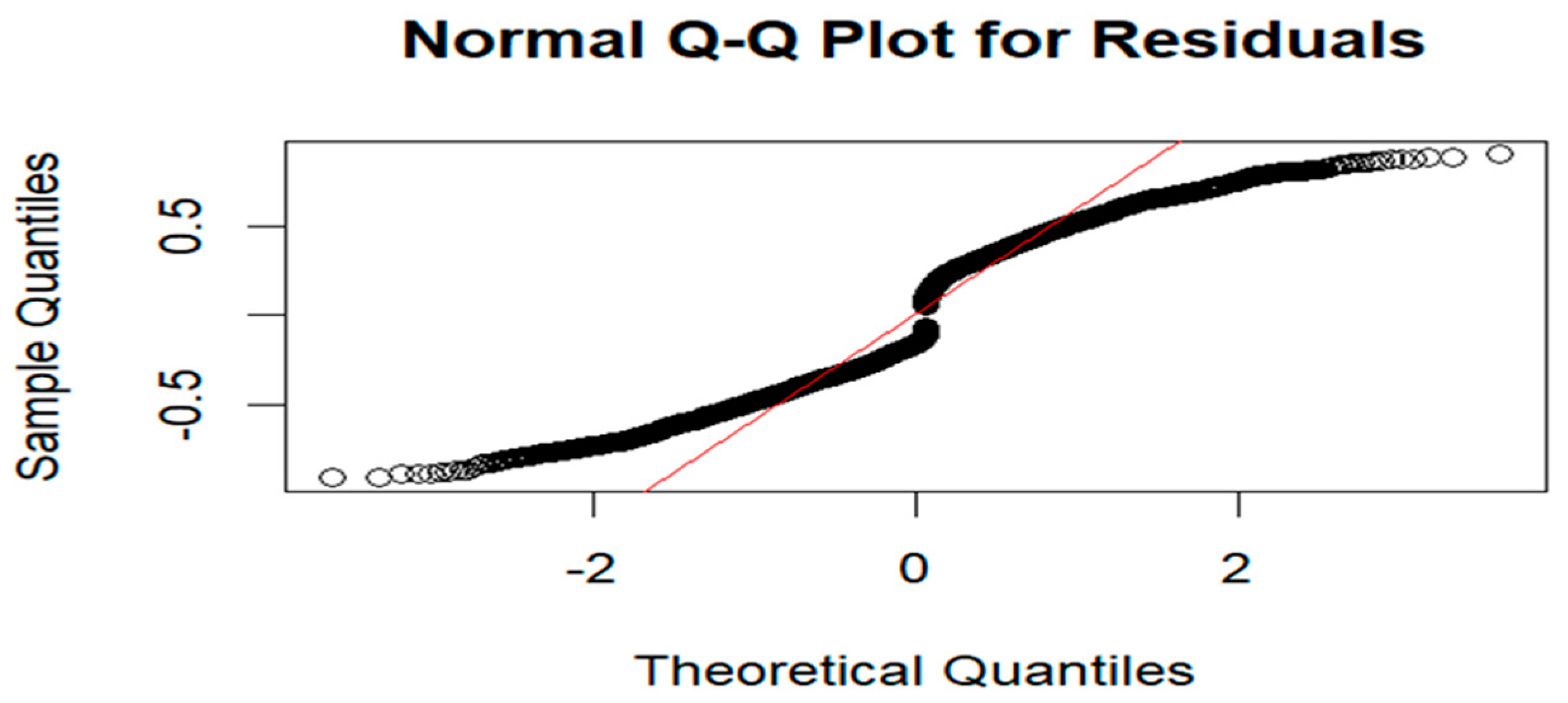
Figure 7.
Variogram Plot for the Residuals.
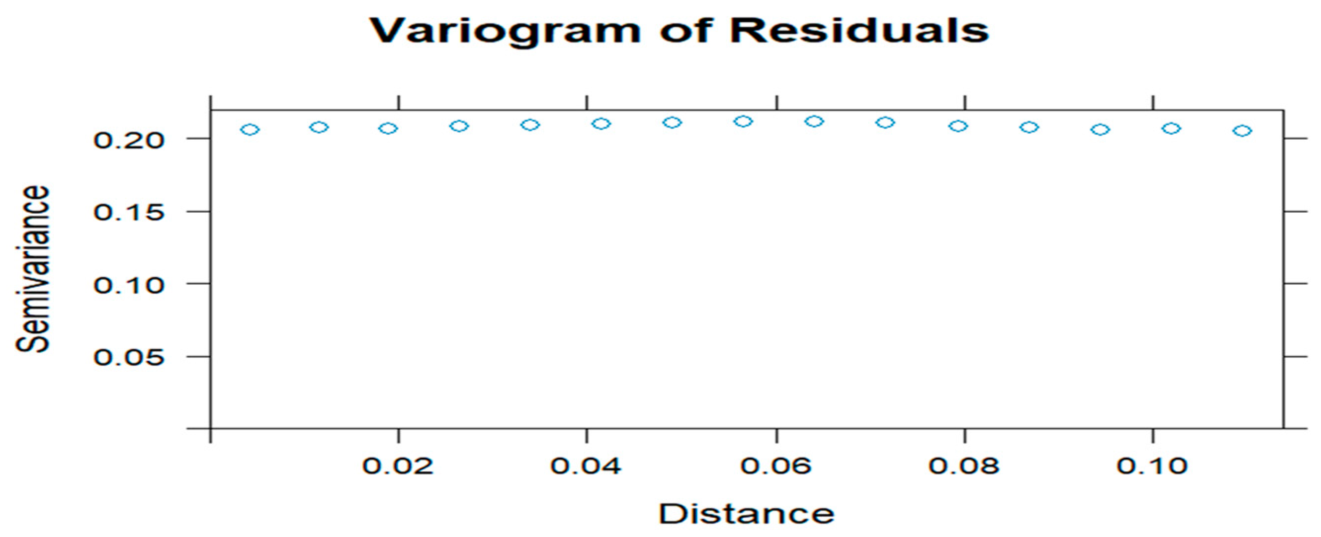
Figure 8.
Posterior density plots for statistically significant coefficients in the model.
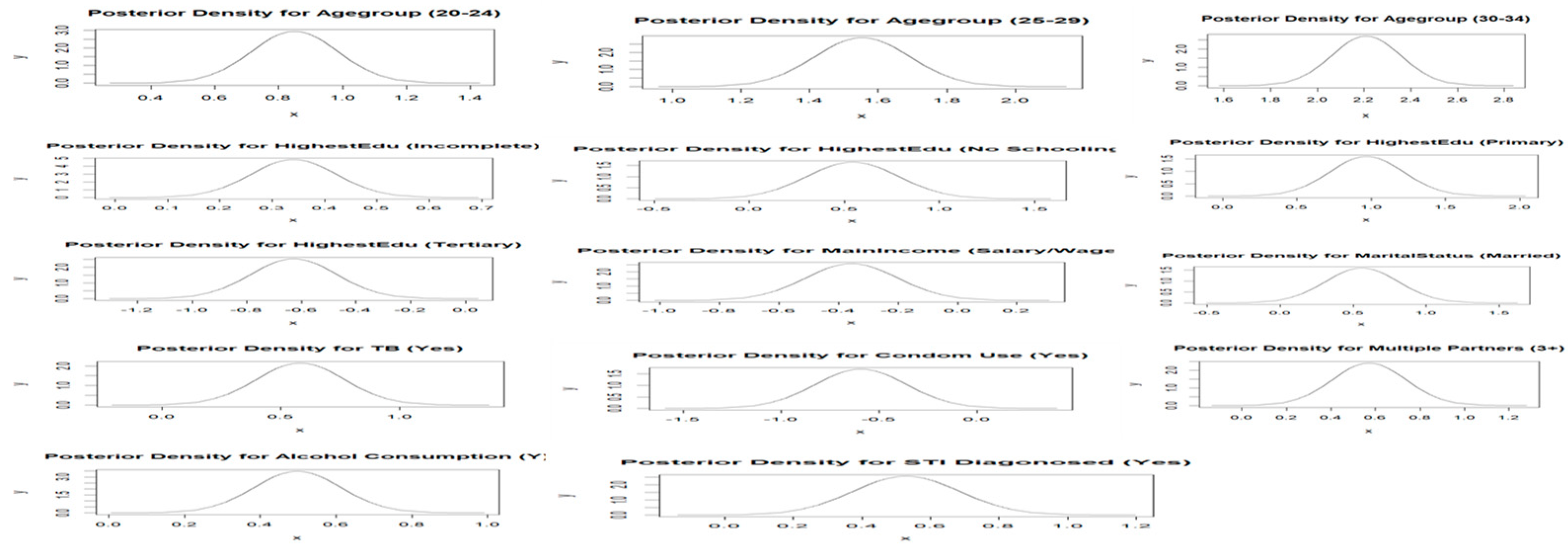

Table 1.
Weighted HIV Prevalence Rates by Each Covariate Among HIV-Positive Females youth in Vulindlela and Greater Edendale Areas in uMgungundlovu Municipality.
Table 1.
Weighted HIV Prevalence Rates by Each Covariate Among HIV-Positive Females youth in Vulindlela and Greater Edendale Areas in uMgungundlovu Municipality.
| Covariate | n = 1576 | HIV Prevalence (%) | 95% CI Lower | 95% CI Upper | -Value |
|---|---|---|---|---|---|
| Age Group | |||||
| 15–19 | 88 | 20.4 | 16.8 | 24.5 | <0.0001 |
| 20–24 | 399 | 37.0 | 34.2 | 40.0 | |
| 25–29 | 546 | 54.0 | 50.8 | 57.1 | |
| 30–34 | 543 | 67.5 | 64.2 | 70.8 | |
| Ever Pregnant | |||||
| No | 282 | 37.4 | 33.9 | 40.9 | <0.0001 |
| Yes | 1294 | 50.4 | 48.4 | 52.3 | |
| Education Level | |||||
| Complete Secondary | 737 | 44.3 | 41.9 | 46.7 | <0.0001 |
| Incomplete secondary (Grade 8-11/NTC1/2) | 660 | 52.1 | 49.3 | 54.9 | |
| No response | 0 | 0.00 | 0.00 | 97.5 | |
| No schooling/creche/pre-primary | 45 | 55.6 | 44.1 | 66.6 | |
| Primary (Grade 1–7) | 60 | 70.6 | 59.7 | 80.0 | |
| Tertiary (Diploma/degree) | 74 | 32.9 | 26.8 | 39.4 | |
| Main Income | |||||
| No Income | 102 | 50.5 | 43.4 | 57.6 | 0.169432 |
| No response | 36 | 49.3 | 37.4 | 61.3 | |
| Other | 0 | 0.00 | 0.00 | 97.5 | |
| Other non-farming income | 102 | 47.9 | 41.0 | 54.8 | |
| Pension or grants | 541 | 50.4 | 47.4 | 53.5 | |
| Remittance (migrant worker sending money home) | 40 | 50.0 | 38.6 | 61.4 | |
| Salary and/or wage | 748 | 44.8 | 42.4 | 47.3 | |
| Sales of farming products | 7 | 50.0 | 23.0 | 77.0 | |
| Marital Status | |||||
| Divorced | 2 | 100.0 | 15.8 | 100.0 | 0.000181 |
| Legally married | 70 | 38.0 | 31.0 | 45.5 | |
| Living together like husband and wife | 56 | 51.4 | 41.6 | 61.1 | |
| Separated, but still legally married | 2 | 100.0 | 15.8 | 100.0 | |
| Single and never been married/never lived together as husband/wife before | 1357 | 47.0 | 45.2 | 48.8 | |
| Single, but have been living with someone as husband/wife before | 86 | 63.7 | 55.5 | 71.8 | |
| Widowed | 3 | 60.0 | 14.7 | 94.7 | |
| Ever diagnosed with TB | |||||
| No | 1482 | 46.7 | 45.5 | 48.5 | 0.000365 |
| No response | 2 | 28.6 | 36.7 | 71.0 | |
| Yes | 92 | 63.0 | 54.6 | 70.8 | |
| Condom use | |||||
| No | 50 | 58.1 | 47.0 | 68.7 | 0.056253 |
| Yes | 1526 | 47.1 | 45.4 | 48.9 | |
| Number of sexual partners | |||||
| 1 | 1278 | 45.5 | 43.6 | 47.3 | <0.0001 |
| 2 | 159 | 51.6 | 45.9 | 57.3 | |
| 3+ | 139 | 67.5 | 60.6 | 73.8 | |
| Alcohol consumption | |||||
| No | 1326 | 45.8 | 43.9 | 47.6 | < 0.0001 |
| Yes | 250 | 58.5 | 53.7 | 63.3 | |
| Ever diagnosed with STI | |||||
| No | 1438 | 46.3 | 44.5 | 48.1 | <0.0001 |
| Yes | 138 | 63.0 | 56.2 | 69.4 | |
| Forced first sex | |||||
| Don’t remember | 26 | 54.2 | 39.2 | 68.6 | 0.246837 |
| No | 1503 | 47.1 | 45.4 | 48.9 | |
| Yes | 47 | 54.7 | 43.5 | 65.4 | |
| Away from home | |||||
| No | 1391 | 47.0 | 45.2 | 48.9 | 0.407053 |
| N response | 7 | 58.3 | 27.7 | 84.8 | |
| Yes | 178 | 50.1 | 44.8 | 55.5 | |
| Length in community | |||||
| Always | 1196 | 46.7 | 44.8 | 48.7 | 0.447987 |
| Moved here less than 1 year ago | 62 | 48.1 | 39.2 | 57.0 | |
| Moved here more than 1 year ago | 315 | 50.1 | 46.1 | 54.1 | |
| No response | 3 | 60.0 | 14.7 | 94.7 | |
| Accessed health care | |||||
| Did not respond | 2 | 33.3 | 4.3 | 77.7 | 0.018296 |
| No | 950 | 45.6 | 43.4 | 47.8 | |
| Yes | 624 | 50.5 | 47.7 | 53.4 | |
| Run out of money | |||||
| Did not respond | 34 | 45.9 | 34.3 | 57.9 | 0.618173 |
| No | 1206 | 47.0 | 45.1 | 49.0 | |
| Yes | 336 | 49.1 | 45.2 | 52.9 | |
| Meal cuts | |||||
| Did not respond | 28 | 40.6 | 28.9 | 53.1 | 0.515632 |
| No | 1259 | 47.5 | 45.6 | 49.4 | |
| Yes | 289 | 47.7 | 43.7 | 51.8 | |
Table 2.
Moran’s I & Geary’s C Summary Statistics.
| Summary Statistics | Moran’s Index | Geary’s C |
|---|---|---|
| Statistic | 0.7067737 | 0.2914347 |
| P-value | <2.2e-16 | <2.2e-16 |
| Expectation | −0.0003052 | 1.000000 |
| Variance | 0.0001070 | 0.0001434 |
| Standard Deviate | 68.361 | 59.176 |
Table 3.
Model Selection Criteria Summary for the Two Competing Models.
| Spatial Logistic Model | DIC | pD | WAIC | |
|---|---|---|---|---|
| Unstructured | 4128.952 | 48.89294 | 4080.059 | 4129.874 |
| Structured | 4127.739 | 40.20267 | 4087.537 | 4128.783 |
Table 4.
Adjusted Odds Ratios and 95% credible intervals for the parameters of the structured model.
Table 4.
Adjusted Odds Ratios and 95% credible intervals for the parameters of the structured model.
| Covariate | OR | 95% CI Lower | 95% CI Upper |
|---|---|---|---|
| Intercept | 0.28880 | 0.0550 | 1.5174 |
| Age Group (ref: 15–19) | |||
| 20–24 | 2.3373 | 1.7914 | 3.0526 |
| 25–29 | 4.7446 | 3.6111 | 6.2339 |
| 30–34 | 9.1981 | 2.8826 | 12.2926 |
| Education (ref: Complete Secondary) | |||
| Incomplete secondary (Grade 8-11/NTC1/2) | 1.4049 | 1.1948 | 1.6520 |
| No response | 0.8001 | 0.1289 | 4.9679 |
| No schooling/creche/pre-primary | 1.7177 | 1.0650 | 2.7732 |
| Primary (Grade 1–7) | 2.6117 | 1.5968 | 4.2759 |
| Tertiary (Diploma/degree) | 0.5337 | 0.3910 | 0.7276 |
| Main Income (ref: No Income) | |||
| No response | 0.8270 | 0.4733 | 1.4448 |
| Other | 0.7929 | 0.1285 | 4.8988 |
| Other non-farming income | 0.8624 | 0.5746 | 1.2943 |
| Pension or grants | 0.8130 | 0.5945 | 1.1107 |
| Remittance | 0.9871 | 0.5764 | 1.6888 |
| Salary and/or wage | 0.7061 | 0.5215 | 0.9560 |
| Sales of farming products | 0.8146 | 0.3009 | 2.2034 |
| Marital Status (ref: Divorced) | |||
| Living together like husband and wife | 0.7305 | 0.2888 | 1.8497 |
| Legally married | 0.3708 | 0.1497 | 0.9185 |
| Single and never been married/never lived together as husband before | 0.9589 | 0,3985 | 2.3071 |
| Separated, but still legally married | 1.7807 | 0.3282 | 9.6504 |
| Single, but have been living with someone as husband before | 1.3539 | 0.5390 | 3.4008 |
| Widowed | 0.8395 | 0.2001 | 3.5184 |
| Ever pregnant (ref: No) | |||
| Yes | 1.1366 | 0.9389 | 1.3744 |
| Run out of money (ref: Did not respond) | |||
| No | 0.9646 | 0.5775 | 1.6112 |
| Yes | 0.9773 | 0.5661 | 1.6871 |
| Meal cuts (ref: Did not respond) | |||
| No | 1.3979 | 0.8245 | 2.3703 |
| Yes | 1.1972 | 0.6805 | 2.1064 |
| TB (ref: Never Suffered from TB) | |||
| No response | 0.6650 | 0.1818 | 2.4303 |
| Yes | 1.7986 | 1.2473 | 2.5935 |
| Condom Use (ref: No) | |||
| Yes | 0.5516 | 0.3482 | 0.8737 |
| Number of Sexual Partners (ref: 1) | |||
| 2 | 1.2117 | 0.9361 | 1.5683 |
| 3+ | 1.7647 | 1.2751 | 2.4449 |
| Alcohol (ref: No) | |||
| Yes | 1.6438 | 1.3100 | 2.0627 |
| STI Diagnosed (ref: No) | |||
| Yes | 1.6938 | 1.2448 | 2.3025 |
| Forced First Sex (ref: Do not remember) | |||
| No | 0.7672 | 0.4334 | 1.3566 |
| Yes | 1.0704 | 0.5283 | 2.1684 |
| Away From Home (ref: No) | |||
| No response | 1.3284 | 0.4757 | 3.7062 |
| Yes | 1.2436 | 0,9753 | 1.5857 |
| Length in Community (ref: Always) | |||
| Moved here less than 1 year ago | 1.0111 | 0.6887 | 1.4859 |
| Moved here more than 1 year ago | 0.9831 | 0.8057 | 1.2008 |
| No response | 1.6989 | 0.4378 | 6.5864 |
| Accessed Health Care (ref: Did not respond) | |||
| No | 1.2918 | 0.4404 | 3.7886 |
| Yes | 1.5762 | 0.5358 | 4.6367 |
Disclaimer/Publisher’s Note: The statements, opinions and data contained in all publications are solely those of the individual author(s) and contributor(s) and not of MDPI and/or the editor(s). MDPI and/or the editor(s) disclaim responsibility for any injury to people or property resulting from any ideas, methods, instructions or products referred to in the content. |
© 2025 by the authors. Licensee MDPI, Basel, Switzerland. This article is an open access article distributed under the terms and conditions of the Creative Commons Attribution (CC BY) license (http://creativecommons.org/licenses/by/4.0/).
Copyright: This open access article is published under a Creative Commons CC BY 4.0 license, which permit the free download, distribution, and reuse, provided that the author and preprint are cited in any reuse.


