

Submitted:
03 February 2025
Posted:
06 February 2025
You are already at the latest version
Abstract
This study seeks to advance the theory of dynamic asset pricing by introducing asset valuation, adjusted by environmental, social and governance (ESG) ratings, within a unified Bachelier–Black–Scholes–Merton market model, and developing option valua tion in both continuous-time and discrete-time (binomial pricing tree) frameworks. An empirical study based on call option prices for assets selected from the Nasdaq-100 develops implied values for the main ESG parameter in the pricing model. For these stocks, option traders have in-the-money ESG valuations that are lower than the spot price. Within the discrete-time framework, we demonstrate how an informed trader can adopt a futures trading strategy to optimize an effective dividend stream.
Keywords:
ESG finance
; Bachelier’s model
; Black–Scholes–Merton model
; option prices
; binomial pricing trees
1. Introduction
Despite initial rejection of the Bachelier model [6], its arithmetic Brownian motion dynamics have found acceptance in certain areas. To combine the strengths of both arithmetic and geometric Brownian motion models, the classical Black–Scholes–Merton (BSM) model [7,27] has been merged with a modernized Bachelier (MB) model [31], producing a unified Bachelier–Black–Scholes–Merton (BBSM) model [25]. Both the unified model and its MB limit allow for price trajectories taking values in , while, under the BSM limit, price processes take values in . Exploiting the more extensive price range of the MB model, [31] developed a dynamic ESG-adjusted valuation (“ESG-adjusted pricing”) for assets, which allows for stocks with low ESG ratings to be given a negative ESG-adjusted value. A critical parameter of the adjusted valuation is the so-called ESG affinity, quantifying the market view of the “size” of the contribution of ESG ratings to asset values. [5] explored fair valuation of options under the MB model using this ESG-adjusted asset valuation.
Consideration of ESG factors in financial modeling marks a paradigm shift in how asset values are assessed. As the world evolves toward a greener future, industry leaders must champion sustainability. (However, see [15] for a study of how sustainability efforts have varied by market). Providing a solid quantitative use for ESG ratings is an important step in the effort to champion sustainability in the financial world. Consideration of ESG-adjusted prices alters the investment approach required for long-term investing, enabling ESG-conscious investors to more effectively measure, and (potentially) profit from, ESG strategies. Analyses based on such pricing must be woven into the investment processes of any discerning investor, as well as integrated into the corporate strategy of any company that is truly committed to increasing shareholder value [21].
The first goal of this paper is to embed ESG asset valuation within the continuous-time BBSM model (Section 2), placing ESG finance within the broader framework of a unified Bachelier and Black–Scholes–Merton theory. In Section 3, we embed the ESG-adjusted asset valuation into the BBSM binomial option pricing model of [25].
The second goal is to provide an empirical study of discrete option pricing under the ESG-BBSM binomial model of Section 3. Our data set for 16 stocks selected from the Nasdaq-100 is described in Section 4.1. Empirical examples of ESG-adjusted prices are presented in Section 4.2. In Section 4.3 we describe how to fit the required parameters of the binomial model to empirical data. In Section 5, using published call option prices for 01/02/2024, we compute implied values of the ESG affinity parameter as functions of strike price and time to maturity. These can then be expressed in terms of an implied ESG valuation (as a function of strike price and time to maturity). Comparing the implied ESG valuation to financial spot prices provides insight into the views of option traders on the impact of ESG ratings on the underlying asset value.
The third goal of this study (Section 6) focuses on a discrete-time, futures trading strategy that can be adopted by an option hedger (the trader taking a short position on an option) who may posses information regarding the future direction of movement of the ESG-adjusted valuation of the underlying stock. While the efficient market hypothesis argues that the direction of the asset price movement is unpredictable [2,3,14,17,18,19,20,23,29], numerous studies challenge this view and indicate that price direction may, indeed, be predictable [1,4,8,9,11,12,24,26,28,30,34,35,36,38,39]. As a result, [10,13,37] and many others have worked on understanding informed trading markets and the strategies employed. We demonstrate that the trader can optimize this trading strategy to produce an effective dividend stream.
Section 7 concludes the paper with a discussion of future directions.
2. Embedding ESG pricing in the BBSM model
Consider the market consisting of a risky asset , a riskless asset , and a European contingency claim (option) . Under BBSM, has the price dynamics of a continuous diffusion process determined by the stochastic differential equation
where is a standard Brownian motion on a stochastic basis
of a complete probability space (). The coefficients satisfy , , , , and are -adapted processes. The -adapted processes and are assumed to satisfy the usual regularity conditions.1 [25] define the appropriate price dynamics2 of the riskless asset in the BBSM market model as
Again, and are -adapted processes. The -adapted process is also assumed to satisfy the usual regularity conditions.3 The MB model is achieved as the limiting case , while the classical BSM model is the limiting case . For brevity, we adopt the notation , and . We require , -almost surely (a.s.). A necessary condition for no-arbitrage is the requirement that , -a.s. Under the no-arbitrage assumption, the market price of risk is
which is strictly positive -a.s. for all providing , -.a.s.
The option has the price dynamics
where , , , has continuous partial derivatives and on , and T is the expiration (maturity) time of . The option’s maturity payoff is for some continuous function . The risk-neutral valuation of is [25]
where is the equivalent martingale measure and the asset price dynamics under is
In (6), , , is a standard Brownian motion on the stochastic basis .
Consider a published ESG rating4 (score) for a company X at time t. argue that bounded scales for an ESG score do not differentiate adequately between the amount of effort that a company must undergo to raise their score above a current value.5 They further argue that scores based upon a convex, monotonically increasing function better represent such effort, and that the choice of such a function should be based ultimately on an axiomatic approach. In the absence of such an approach, they proposed the relative ESG measure
where is the ESG rating (score) of company X and is the ESG score of a relevant market index I.6 They further define the ESG-adjusted stock price of company X at time by
which incorporates ESG scores as part of an asset’s valuation. Here represents the financial price of an asset, while represents an ESG-adjusted valuation,7 which refer to as the ESG-adjusted price. In (8), is referred to as the ESG affinity of the financial market.8
The ESG-adjusted stock price (8) can be negative.9 This is not surprising as the relative score is analogous to any financial `spread’. We note the following dependencies of on .
From (9a) through (9d), we see that changing the value of only affects the (additional) fractional financial price term , which satisfies .
3. Binomial Option Pricing under the BBSM Model
[25], Section 7 developed a binomial option pricing model under the BBSM model. We briefly summarize that model here. Consider a BBSM market ) consisting of the risky asset (stock) , the and call option . The stock price evolves according to the binomial pricing tree
In (10), , is the stock price at time , where T is the fixed maturity time and . For every , , , are independent, identically distributed Bernoulli random variables with determining the filtration
of the stochastic basis on the complete probability space . The riskless asset has the discrete price dynamics
where is the instantaneous rate of (2) at times .
Under BBSM, price changes, rather than returns, are of primary interest. Let
Then,
In order that the càdlàg process on the Skorokhod space generated by the binomial tree (10) converge weakly to the continuous time process (1), we require that the conditional mean and variance satisfy
where and are the instantaneous mean and variance of (6) at time . Then and are given by
The option has the discrete price dynamics , . Consider a self-financing strategy, replicating the option price process :
The standard no-arbitrage arguments lead to
Thus, the risk-neutral valuation of the option is given by the recursion
where the risk-neutral probability is
The limit of (18) and (19) produces the option price recursion relation for the BSM model,
having risk-neutral probability
where is the discrete form of the market price of risk, , in the BSM model.10 In this limit, the discrete price of the riskless asset obeys, .
The limit , produces the option price recursion relation for the [31] Bachelier model,
The risk-neutral probability is (see also [22]),
In this limit, the discrete price of the riskless asset obeys .
3.1. The Binomial Model is Not Recombining
A careful analysis shows that the risky-asset asset price process (10) does not, in fact, form a recombining tree. For a fixed value of k, , the superscripts and determine node “level” values at time . For a recombining binomial tree, at time k, there are level numbers Thus each node on the tree is indexed by a pair, , . With the inclusion of level numbers, (10) is written as
where, from (16),
Figure 1 illustrates a price configuration on four nodes of the tree, with time and level values indicated. Substituting (25) into (24) gives
where
Note that , , , and are constants.
For the tree to be recombining, in Figure 1 we must have
With some algebra, the difference
can be shown to be
independent of time or level number.11 To ensure that the tree is numerically recombining in our empirical work in Section 4, we define
We note that vanishes more rapidly than and terms as . However, theoretical work remains to be done to ascertain whether the càdlàg process on the Skorokhod space generated by either (10) or (30) does indeed converge weakly to the continuous time process (1). We leave this question open for further investigation. We do note that the BSM and MB limits of the price process (10) are indeed recombining (binomial) trees whose generated càdlàg processes do converge weakly to the appropriate BSM and MB limits of the continuous time process (1).
4. Empirical Examples: ESG-adjusted Prices and Parameter Fitting
4.1. The Data
Table 1 provides brief summaries of the 16 companies in the Nasdaq-100 index (^NDX) as of 01/02/2024 that we considered for our empirical study.12
Adjusted closing prices for the period 01/04/2016 through 01/02/2024 were obtained for these stocks from Yahoo Finance.13 ESG scores for all 101 asset class shares in ^NDX were obtained from Bloomberg Professional Services.fn:accessed Bloomberg provides “fiscal year” ESG scores.14 On 01/02/2024, yearly ESG scores were available for FY 2015 through FY 2022; scores for FY 2023 had not yet been released. Therefore the ESG scores for FY2023 were set equal to those for FY2022. Individual stock weights for the ETF Invesco QQQ Trust, Series 1 were used as proxies for actual ^NDX weights.15 In our view this is a preferable choice for the weights as the ETF is a tradeable instrument that is designed to track the ^NDX.
Using the QQQ weights, a weighted ESG score for ^NDX was computed for each fiscal year. Figure 2 shows the resultant fiscal year, relative ESG scores of the 16 chosen companies. Seven of the stocks have positive relative ESG scores over the entire 8 years of data; eight have negative relative ESG scores; and only one, PANW, has an ESG score that increases from below the index value to above. We note that, with the exception of PANW, the change in the ESG score of most companies relative to the index weighted average has remained approximately constant, or decreased, since 2019.
The ESG data were smoothed to provide daily values. Specifically we smoothed the values of . The fiscal year values were assigned to the last day (December 31) of the year (with the ESG score for 01/02/2024 being set equal to the 12/31/2022 value). The daily smoothing, which consisted of two steps: linear interpolation followed by a Gaussian-weighted, moving average smoothing function, provided daily values between 12/31/2015 and 01/02/2024. The linear interpolation produced daily values between successive year end values. The Gaussian-weighted, moving average produced a smoother curve having the property that it produces no data “overshoot” or “undershoot”. Figure 3 shows an example of the smoothing for .
4.2. ESG-Adjusted Prices
In Section 5, implied values for were estimated from call option prices, reflecting the view of option traders. However, there is no estimate for values of based upon historical spot trading. In order to investigate historical ESG-adjusted prices, we proceeded as follows. We assumed that the financial price series for each stock X over the historical time period 01/04/2016 though 01/02/2024 is a semi-martingale – most probably a Lévy process. Using the historical price series, we computed the time series of ESG-adjusted prices (8) over the range of parameter values . For each value of , we determined the signal:noise ratio, , of . Figure 4 shows plots of for four example stocks, illustrating a range of behaviors.
Defining and by
determines a range of values for which lies withing 5% of the value . We assumed that as long as the s:n ratio of the ESG-adjusted price remains within this range, the time series will continue to be a semi-martingale.16
The range found for each stock is given in Table A1 in Appendix A. The ranges vary, sometimes significantly. For the four stocks represented in Figure 4, Figure 5 plots the ESG-adjusted price series for . For PANW, the s:n ratio changes rapidly near , and the range is very narrow. WBD and ASML illustrate that the s:n ratio can remain within 5% of s:n(0) for extended ranges of either or . The results for AMD are representative of 13 of the 16 stocks for which . For AMD and ASML, (Figure 2) over the historical time period; as a consequence the ESG-adjusted price increases with . For WBD, and its ESG-adjusted stock price decreases as increases. PANW is the only stock of the 16 companies considered whose ESG score increased from below to above that of ^NDX. The and curves therefore cross each other near the start of 2022 (difficult to visualize in the plot for PANW in Figure 5).
4.3. Parameter fits
To compute option prices using the binomial BBSM model in Section 3, predictive empirical ESG-adjusted prices (10) were computed assuming constant parameter values. Section 9 [25] suggested (but did not implement) procedures for fitting the parameters of a BBSM model. With minor modification, we follow their suggested procedure for estimating the risky-asset price parameters; we utilize a different procedure for estimating the riskless asset price parameters. The parameter values were estimated from the historical price data, as follows. Express the historical data as the trading dates (), where corresponds to 01/04/2016 and to 01/02/2024.17 From (15) with constant coefficients, the conditional mean and variance of the discrete change in stock price are
The parameters a and were obtained using the regression
Using the approximation , the parameters v and were estimated from the regression
With constant parameters, the price dynamics (12) of the riskless asset has the discrete form18
The parameters and r were estimated from the regression
The sequence of daily values required in (36) was generated as follows:
where is the three-month U.S. Treasury bill rate, converted to a daily rate.19,20
Finally, we estimated the probability for the upward movement of the daily ESG-adjusted closing price by
where the indicator function satisfies if and otherwise.
From (8), for each time t there exists a value such that . Therefore if , a time independent constant over the historical period for which the regression fits (33) and (34) are to be attempted, the linear regressions near the value become ill-conditioned and unrealistic parameter fits result. As we utilized an eight-year historical window over which had behaviors similar to that illustrated in Figure 3, this was not an issue.
Figure 6 shows the dependence of the values of the fitted parameters , , , , , , on for ASML and ROST.
These are illustrative of the forms of dependence seen in the 16 stocks. In the plots for , the black curve indicates the value of estimated using (38). A change in the value of by its smallest increment () as changes is visible as a corresponding jump in the value of . We used a Gaussian-weighted, moving average smoother (with a window of 21 days) to smooth the values (red curve).
In (37) the value of only affects the value of . Consequently, in the fit (36) we see from Figure 6 that the parameter depends on , while the parameter r is independent of the value . In fact the constant fitted value of is independent of the stock considered, which makes sense as, except for an initial value , (37) and (36) depend only on the riskless asset.
Figure 6 shows that, with the exception of , as varies over the range , each fitted parameter varies over a range of values, with the range varying by stock. For each fitted parameter, Figure 7 compares, by stock, the range of values taken on by that parameter. Dotted horizontal lines are used to guide the eye to separate positive from negative paramater ranges, or, in the case of , to indicate stocks having . We note that the range for each stock includes (no ESG price adjustment). Even so, the MB parameters , and are consistently different from 0 over the full range (except for for WBD). Thus the parameter fits, even for the financial stock price (), show an admixture of MB and BSM behavior. The values of and are positive for all 16 stocks; for all values are negative. For , all are negative except for two stocks, NVDA and PANW. Values of are equally divided between positive and negative over the 16 stocks. Values of exceed 0.5 for all stocks except WBD.
5. The Implied ESG Affinity
Let denote published call option prices for an underlying stock having maturity date , , and strike price , . Let denote the call option price computed from Section 3 with constant parameters values. Let denote the historical estimation of any parameter . (Recall that, except for , the parameters have dependence on the value of .) Then implied values for are computed via
Based upon call option prices published on 01/02/2024,21 we computed theoretical call option prices for the same set of strike prices, , , and maturity times , . In (39), the parameters used in the theoretical option computation were fit from the historical data for each value of tested in the minimization procedure. As the value of is independent of the value of and of the stock, theoretically it only needed to be calculated once. However, it is computed from the same regression (36) that produces , so it was recomputed for each value of tested. The value used to compute prices on the binomial tree was the smoothed value for 01/02/2024.
The published call option prices for AAPL on 01/02/2024 are presented in Figure 8.22 In contrast to some of the other stocks investigated, these option prices form a fairly “regular” surface over the published range of , , and maturity times , values. The values computed from (39) are plotted as a surface in Figure 8.23 Analysis of the surface is enhanced by consideration of surface contours as shown in the bottom left of the figure. The contour lies between the contours and , indicating that option traders have a positive view (relative to ^NDX) of the ESG rating of AAPL in the upper left triangular region of out-of-the money (the adjusted closing price for AAPL on 01/02/2024 was $185.64) strike prices and maturity dates not exceeding 110 trading days. However, over the majority of values, the option traders have a negative view of the ESG rating of AAPL.
A further view of the values is presented in Figure 8 as a box-whisker summary of the distribution over the surface. Table A1 in Appendix A presents the numerical values of the minumum, maximum, , , and percentiles of the distribution for AAPL. This table also presents the for AAPL based upon examination of historical adjusted ESG prices discussed in Section 4.3. The overwhelming majority of values lie within the for AAPL, giving some confidence that the implied ESG affinity values being computed are consistent with semi-martingale behavior of the associated ESG-adjusted price.
To appreciate the implication of this, we define from (8) an implied ESG-adjusted price
where, for a given stock X, is a value from the implied ESG affinity surface, and was the relative ESG score and the spot price price used in computing the surface.
Figure 9 presents the surface of values computed from the values of Figure 8. Also shown are contour levels of the corresponding to the analogous contour levels of shown in Figure 8. Whether is larger or smaller than depends on the sign of the product . If is positive, then positive values of correspond to an ESG valuation that exceeds . However, if is negative, then negative values of correspond to an ESG valuation that exceeds . Thus, consideration of the surfaces rather than the surfaces provides direct insight into the views of option traders on the ESG-valuation of stocks.
Since was positive on 01/02/2024, the surfaces of and are identical except for a rescaling of the z-axis. Similarly the contour plots for and are identical except for a rescaling of the value on the contour levels. The negative view of the option traders over most of the range for AAPL, results in implied, ESG-adjusted prices for 01/02/2024 that correspondingly fall below the financial price of AAPL on 01/02/2024.
Figs. Figure A1 and Figure A2 in Appendix B plot the published option prices on 01/02/2024 for all 16 stocks studied. The eight stocks for which on 01/02/2024 are presented in Figure A1, while the eight stocks for which are presented in Figure A2. This separation reflects the fact that when , the corresponding surfaces for and will look like identical (rescaled) versions of each other. However, when , the surface will look like an inverted, rescaled version of the corresponding surface. Examination of published option prices for PANW, TEAM, and WDAY show much greater irregularity over the range of K and T values than that shown for AAPL.24
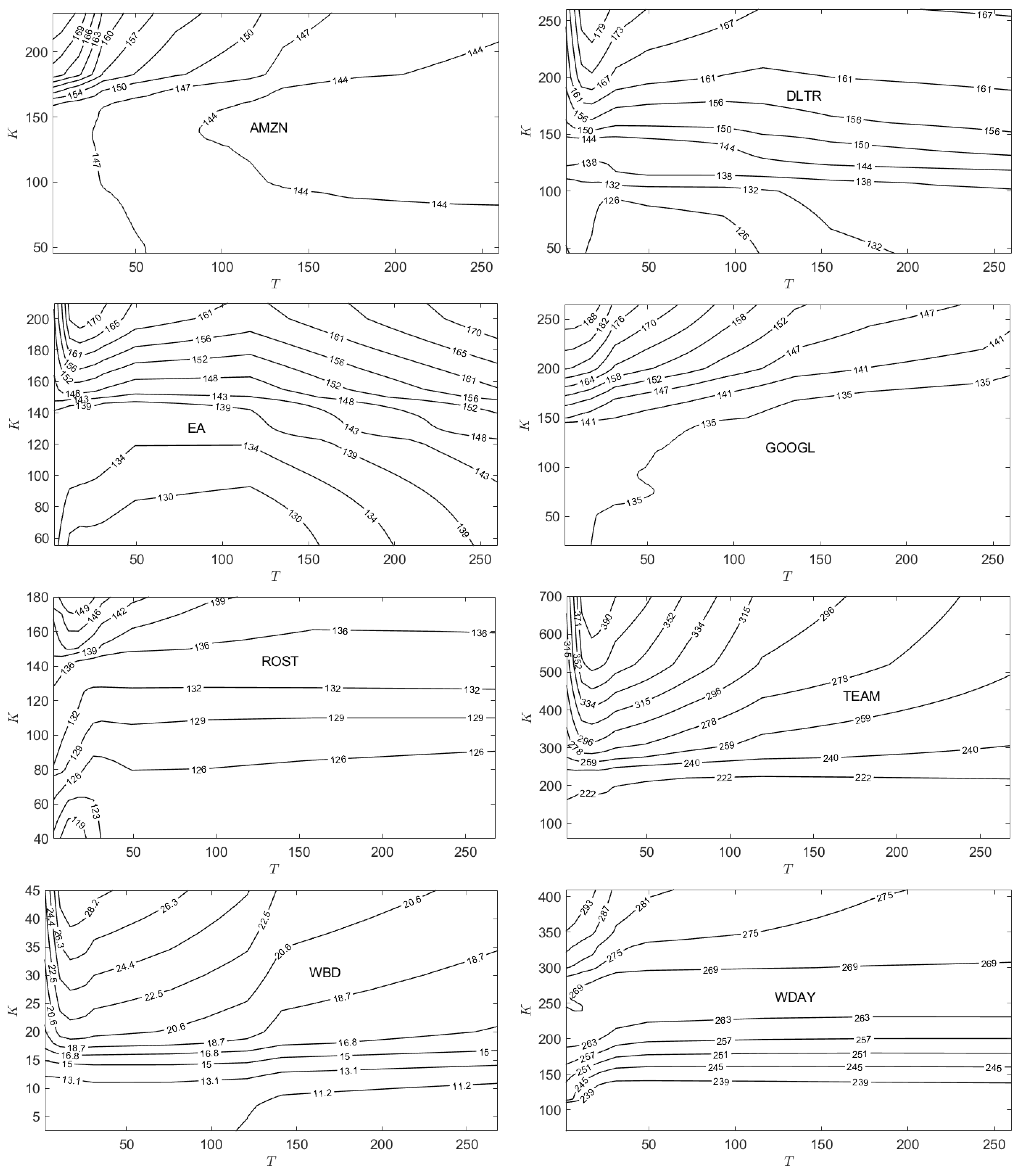
Plots of the surfaces for all 16 stocks are presented in Figs. Figure A3 and Figure A4 in Appendix C. The stock organization into two panels mirrors that for Figs. Figure A1 and Figure A2. Figs. Figure A5 and Figure A6 provide the contour plots of these surfaces. Plots of the surfaces for all 16 stocks are presented in Figs. Figure A8 and Figure A9 in Appendix D. Figure A10 and Figure A11 provide the contour plots of these surfaces.
To summarize the information in Appendix C and Appendix D, Figure 10 presents the box-whisker summaries of the distributions of values for each of the 16 stocks. (The corresponding box-whisker summaries of the distributions of values are given in Figure A7.) Also indicated just to the left of each box-whisker summary is the financial spot price of the stock on 01/02/2024. For ease of reference, the financial spot prices on 01/02/2024 are listed in Table A2. From the contour plots in Figure A10 and Figure A11, one can then ascertain over what region of values option traders view the ESG valuation of the stock to be higher than its financial price. For EA, INTC, TEAM and WBD, spot traders have an implied ESG valuation that exceeds the spot price over most of the region. For eight of the stocks (AAPL, AMAT, AMD, AMZN, ASML, CSX, NVDA, PANW), the implied ESG valuation exceeds the spot price over a triangular, out-of-the-money, shorter maturity time region as described above for AAPL. For the remaining four stocks, the implied ESG valuation exceeds the spot price over most of the out-of-the-money region. Thus, for 12 of the 16 stocks, option traders have in-the-money ESG valuations that are lower than the spot price.
6. Trading Forward Contracts Utilizing Information on Asset Price Direction
[22] extended BSM-based binomial option pricing theory to complete markets containing traders that have information on the stock price direction. We further extend that theory using the BBSM-based binomial option pricing in complete markets of Section 3. For simplicity, we assume the parameters in the BBSM binomial model are constant: , , , , , and , . As earlier, we continue to assume is constant.
Let ℵ denote the trader (hedger) holding the short position in the option contract. Let denote the probability that information held by ℵ at time , , on the direction of stock price movement within any interval is correct. If , ℵ is an informed trader; if , ℵ is misinformed; and if , we refer to ℵ as a noisy trader. We assume ℵ is the only informed trader in a market of noisy traders; consequently, ℵ’s informed trading actions do not influence market prices.
In [22], Shannon’s entropy [see e.g., [32,33] is used to quantify the amount of information ℵ possesses. As with the price movement probability of Section 3, is the probability governing a Bernoulli random variable such that . Then Shannon’s entropy is , having maximum value . [22] defined ℵ’s level of information as25
where
We address the question of ℵ’s potential gain from trading with an information level . At any time , , ℵ makes independent bets, , . Thus, the filtration (11) needs to be augmented with the sequence of ℵ’s independent bets:
Specifically, relying on the information on stock-price direction, ℵ adopts a trading strategy involving forward contracts. For convenience, we label the two scenarios given by (10) for the price of :
: , resulting in w.p. ,
: , resulting in w.p. ,
where and are given by (16) with constant coefficients. If at , ℵ believes that will happen, ℵ takes a long position26 in -forward contracts, for some .27 The forward contracts mature at . If at , ℵ believes that will happen, then ℵ takes a short position in -forward contracts26:oppparty having maturity .
[25] developed the price of a forward contract under the BBSM model. Assuming there is no initial cost to enter into the forward contract and constant coefficients, the T-forward price of is
where the constant coefficient solution to (2) is [25], (A3)]
Evaluating (44) using (45) gives
for all . Discretizing (46) over the time interval and assuming , (46) becomes
For notational brevity, define .
Using (10), conditionally on , the payoff possibilities of ℵ’s forward contract positions can be written
The conditional expected payoff is
with and given by (16).
We write
where, , for any finite value of . is referred to as ℵ’s information intensity. Again assuming ,28
Under the same assumption, the conditional variance of ℵ’s payoff is
The instantaneous information ratio is then
As is positive, the information ratio on the payoff of ℵ’s strategy increases: as ℵ’s information intensity increases, and when .29
To hedge the short position in the option, ℵ executes the positions (17), while simultaneously running the futures trading strategy. This leads to an enhanced price process for ℵ, the dynamics of which can be expressed as:
, . The price change of the process (54) is
Conditionally on , and using (16),
It is in ℵ’s interest to find the value of which maximizes the conditional Markowitz’ expected utility function,
where is ℵ’s risk-aversion parameter. Using (56), is maximized for
Under the optimal value,
and the instantaneous conditional market price of risk for ℵ is
If ℵ had not traded futures on the information possessed, the trader’s instantaneous conditional market price of risk would have been the same as a noisy trader:
Thus, futures trading results in an (optimized) dividend yield over the time interval determined by the solution of
Thus,
We note that, relative to a noisy trader,
Equality between the first and last terms in (64) is obtained for or since, under these limits, all traders become aware of the direction of the price movement.
We investigate the dividend payout as a function of and . From (59) we note that is a monotonic function of having the limits and . Under the limit , which corresponds to sufficiently small values of or sufficiently large values of ,
which is always positive, increasing with and decreasing as increases. Under the limit , which corresponds to sufficiently large values of or sufficiently small values of ,
In this limit, the dividend payout is essentially independent of .
7. Conclusion
Dynamic asset pricing based upon geometric Brownian motion [7,27] has had a tremendous’ impact on finance theory. While having had difficulty gaining acceptance, dynamic pricing based upon arithmetic Brownian motion [6] has certain attractive features. The unified BBSM model of [25] encompasses the strengths of both models. By adapting the BBSM framework to a model of ESG-adjusted asset valuation, we put the full strength of the BBSM model to practical use. Using an empirical data set of 16 stocks taken from the Nasdaq-100, based on call option prices for 01/02/2024 we have shown that, generally, option traders were implying ESG-adjusted prices that exceed the spot price in the out-of-the-money region, while in-the-money, ESG-adjusted prices were lower that the spot price. A follow-up study is required to determine how universal an observation this may be. It would be interesting to investigate call option prices issued during periods of bull and bear markets, and during market disruptions.
We have further extended this ESG-BBSM model to consider futures trading strategy accessible to a trader ℵ holding information on the direction of ESG-adjusted prices. It would be of interest to evaluate ℵ’s optimal dividend payout by, for example, projecting it forward on the binomial tree and computing an expected dividend at time . While this could be evaluated for a specific asset, using historical estimated values , , , , , , , and a spot price (with ), there is no historical information available for , while the parameters and are trader-dependent. Thus, estimates of an expected averate dividend payout at require an investigation of a three dimensional phase space - a fairly daunting prospect best left for a separate study.
Appendix A. Tables
Appendix A.1

Table A1.
Historical range and option price distribution summary statistics.
| Ticker | Min | Max | ||||
|---|---|---|---|---|---|---|
| AAPL | ||||||
| AMAT | ||||||
| AMD | ||||||
| AMZN | ||||||
| ASML | ||||||
| CSX | ||||||
| DLTR | ||||||
| EA | ||||||
| GOOGL | ||||||
| INTC | ||||||
| NVDA | ||||||
| PANW | ||||||
| ROST | ||||||
| TEAM | ||||||
| WBD | ||||||
| WDAY |
Table A2.
Adjusted closing prices on 01/02/2024 for the 16 stocks studied.
| AAPL | AMAT | AMD | AMZN | ASML | CSX | DLTR | EA |
|---|---|---|---|---|---|---|---|
| 185.64 | 154.37 | 138.58 | 149.93 | 716.92 | 34.62 | 142.54 | 135.78 |
| GOOGL | INTC | NVDA | PANW | ROST | TEAM | WBD | WDAY |
| 138.17 | 47.80 | 481.68 | 288.92 | 137.68 | 226.67 | 11.66 | 268.28 |
Appendix B. Plots of Empirical Option Data C(emp)
Figure A1.
for which on .
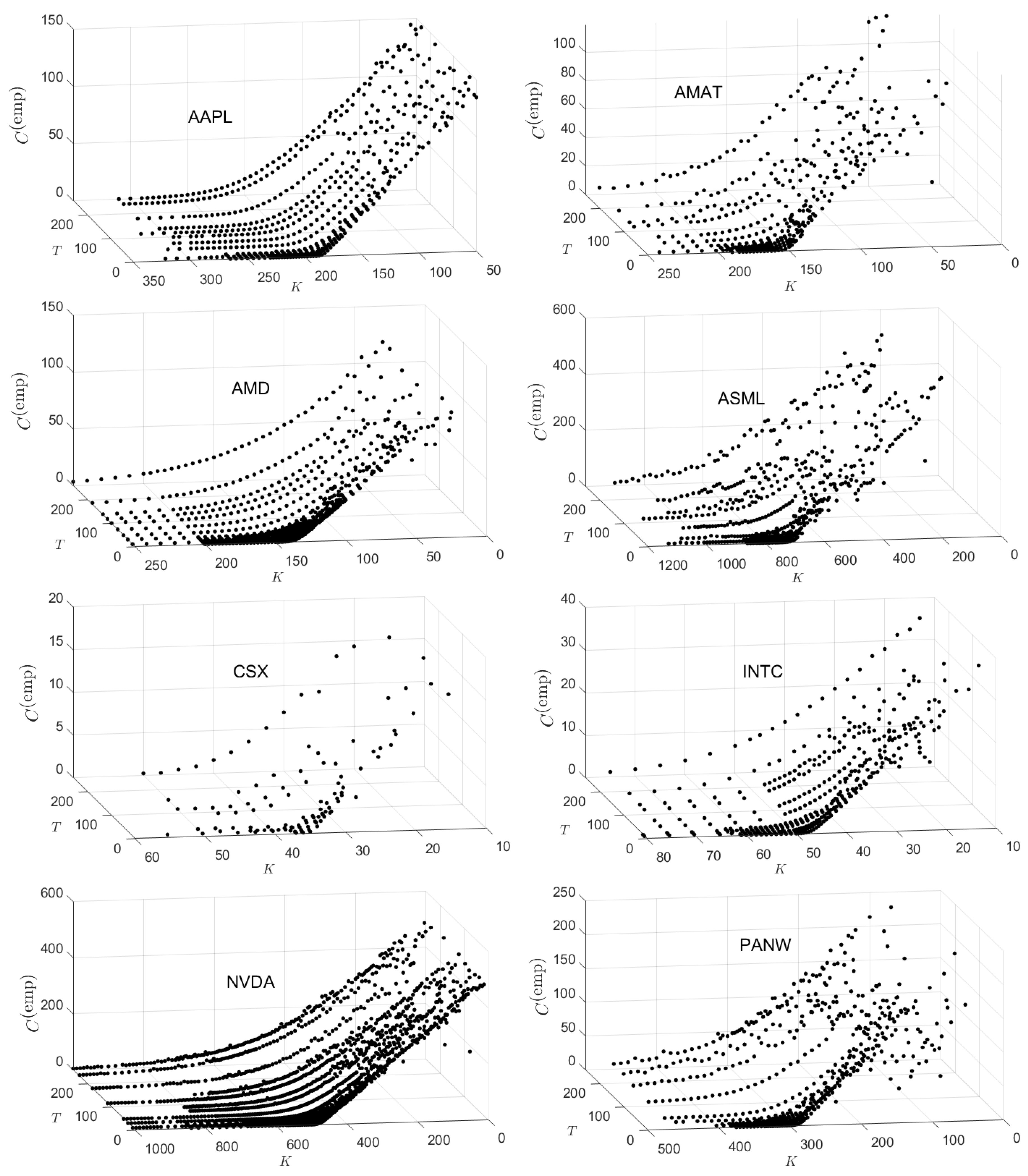
Figure A1 plots the empirical call option contract prices as a function of strike price K and time to maturity T for the eight companies for which for while Figure A2 plots the same for the eight companies for which for
Figure A2.
for which on .
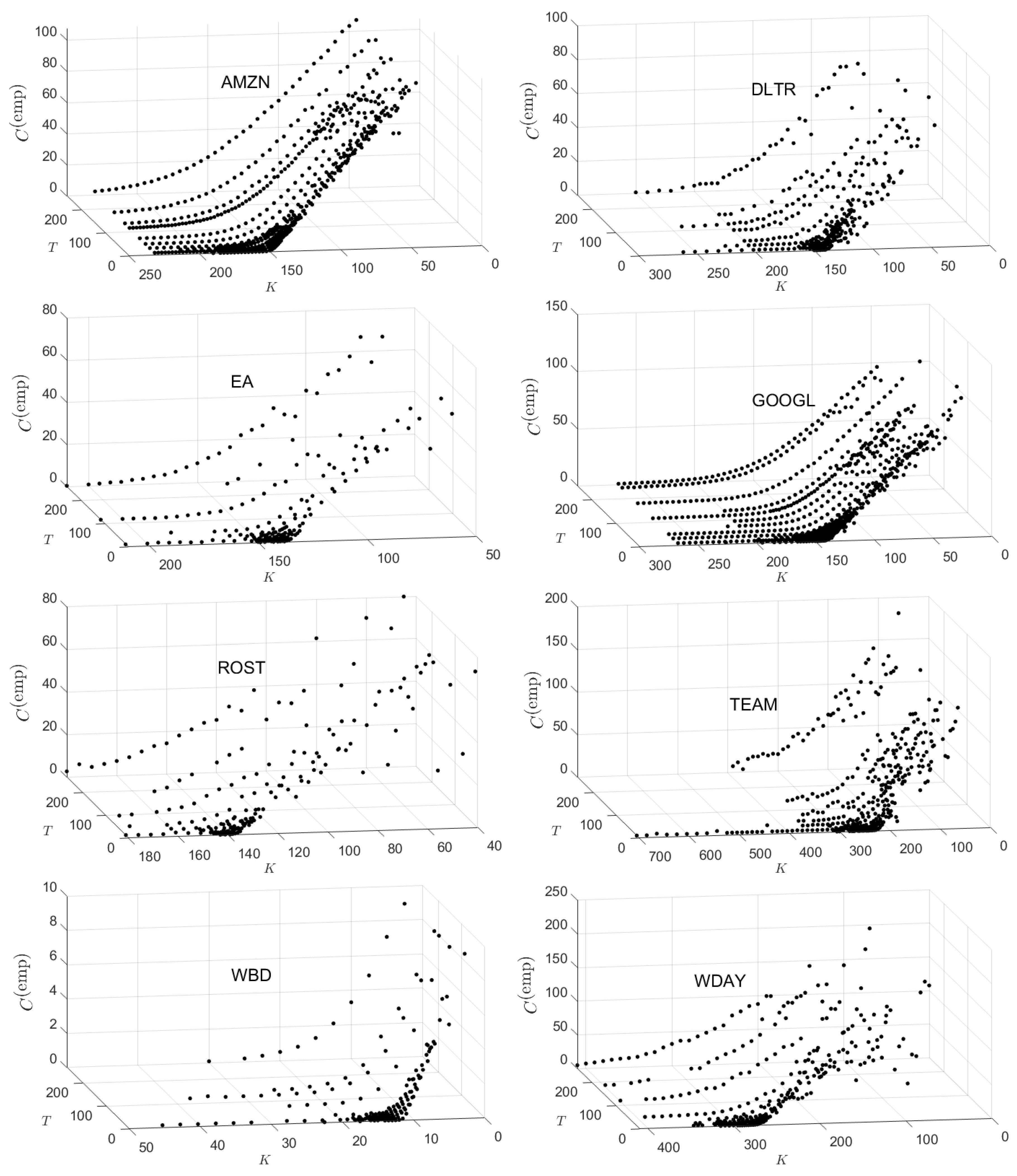
Appendix C. Plots of γ(ESG,imp)
Figure A3.
The implied surfaces for which on .
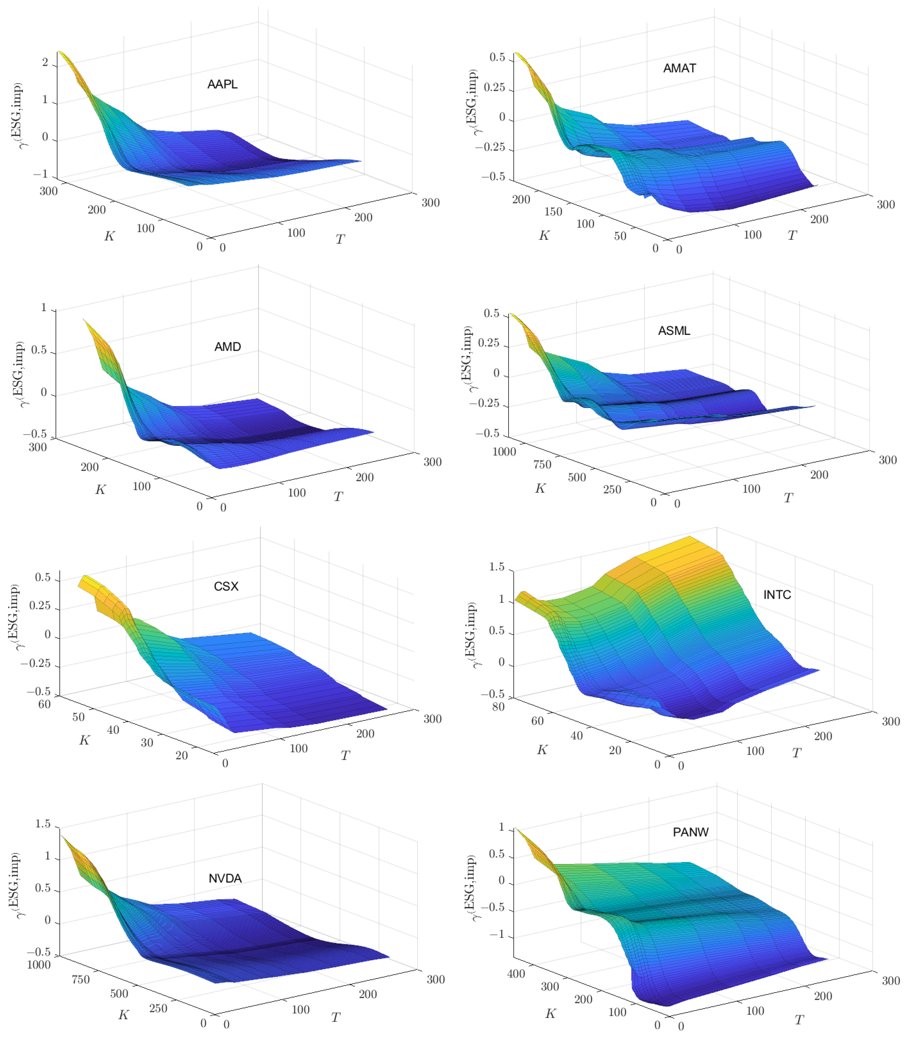
Figure A3 plots as a function of strike price K and time to maturity T for the eight companies for which on .
Figure A4.
The implied surfaces for which on .
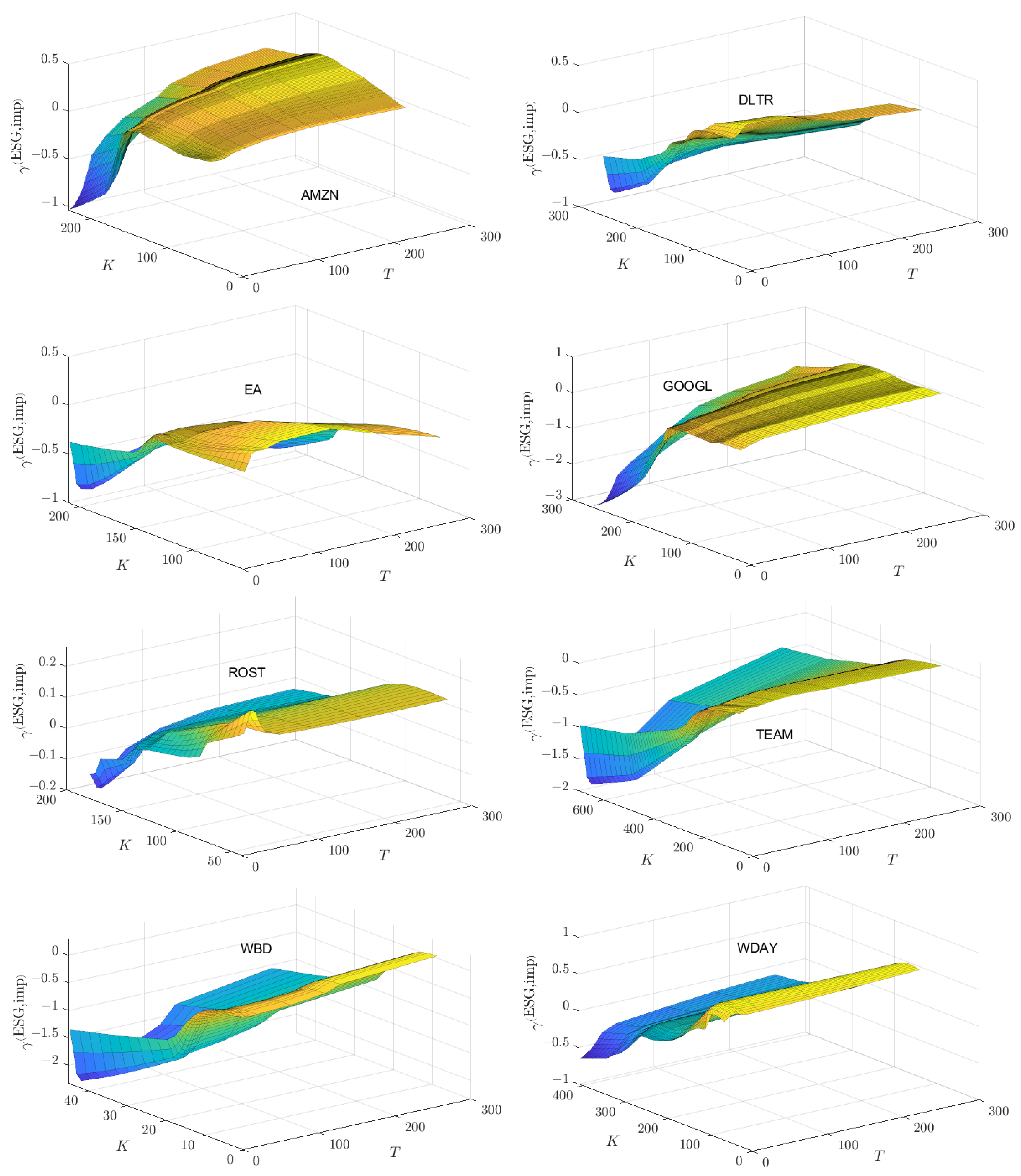
Figure A4 plots for the eight companies for which on .
Figure A5.
Contours of for which on .
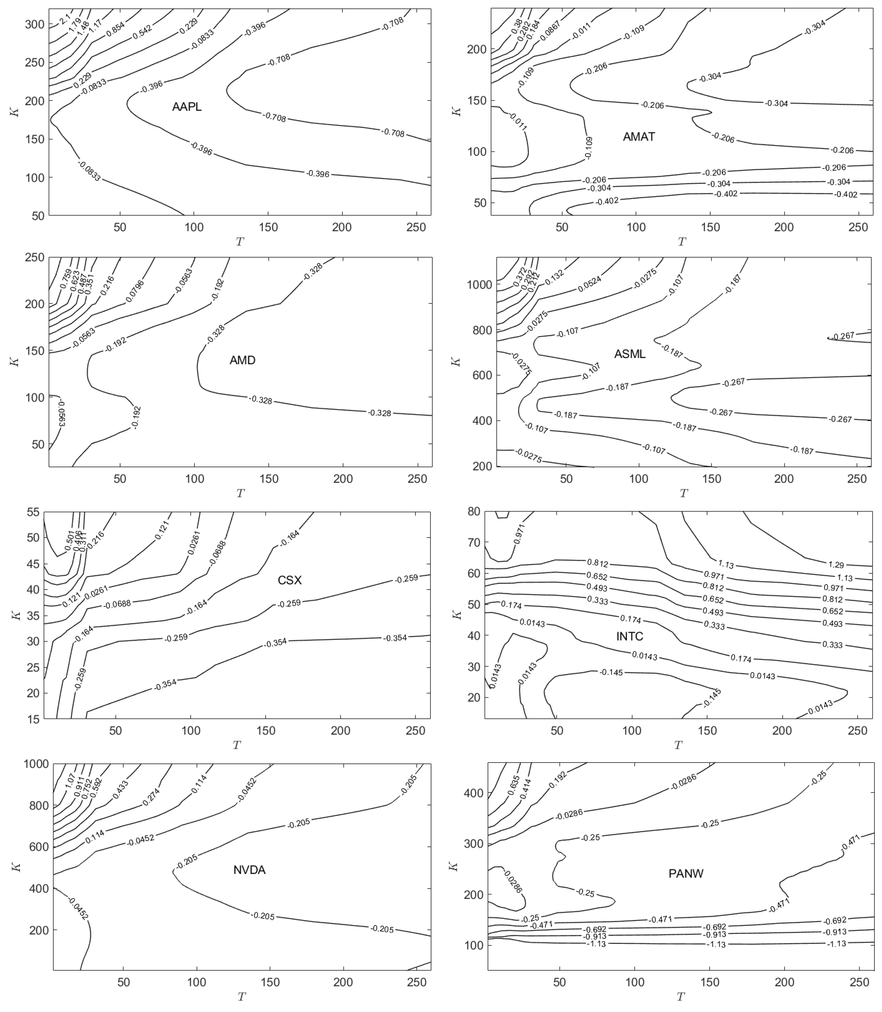
Figure A5 plots contours of as a function of strike price K and time to maturity T for the eight companies for which for , while Figure A6 plots the same for the eight companies for which for
Figure A6.
Contours of for which on .
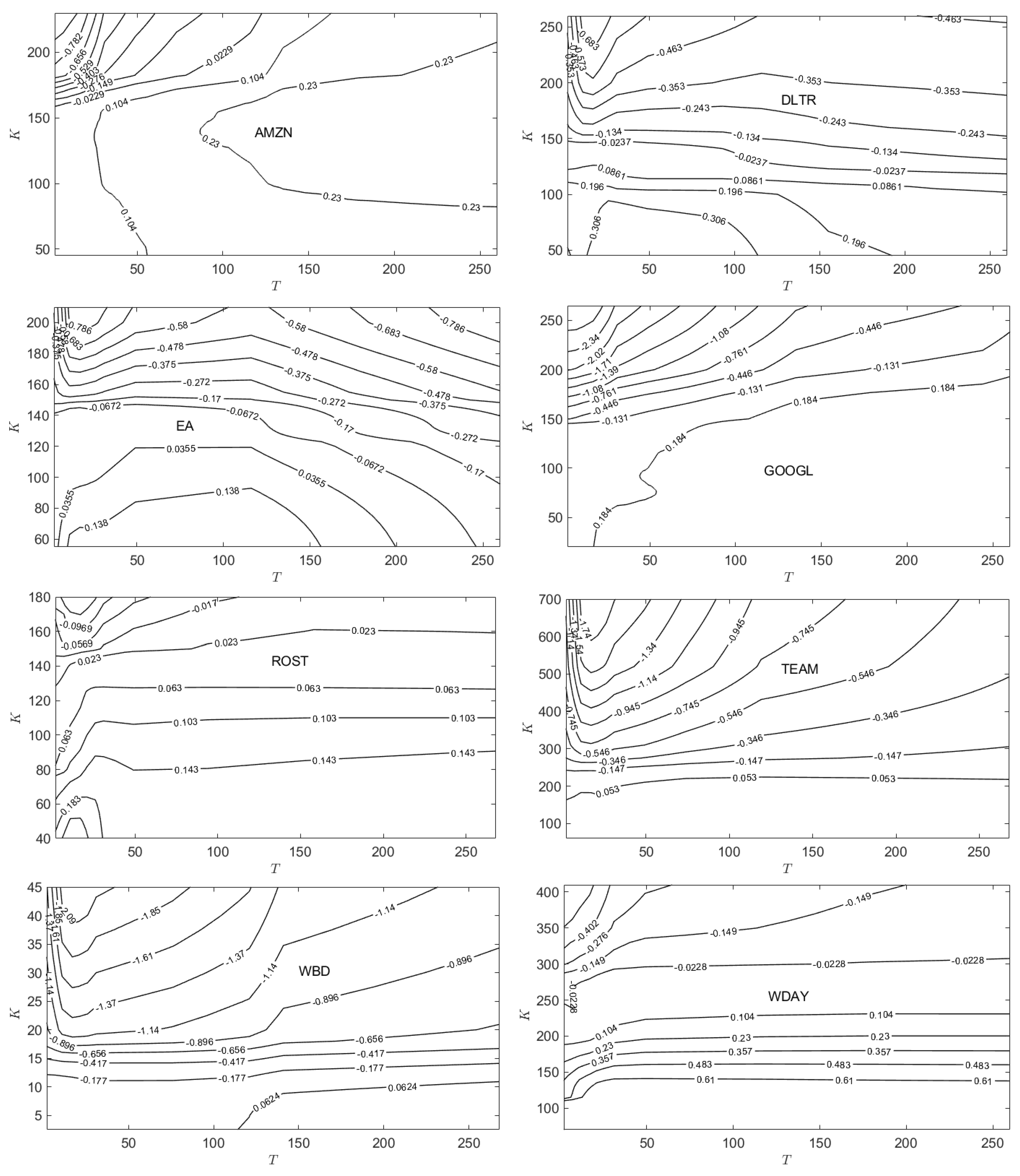
Figure A7.
Box-whisker summaries of the distribution of values for all 16 stocks studied. The horizontal dotted-line indicates the value .
Figure A7.
Box-whisker summaries of the distribution of values for all 16 stocks studied. The horizontal dotted-line indicates the value .
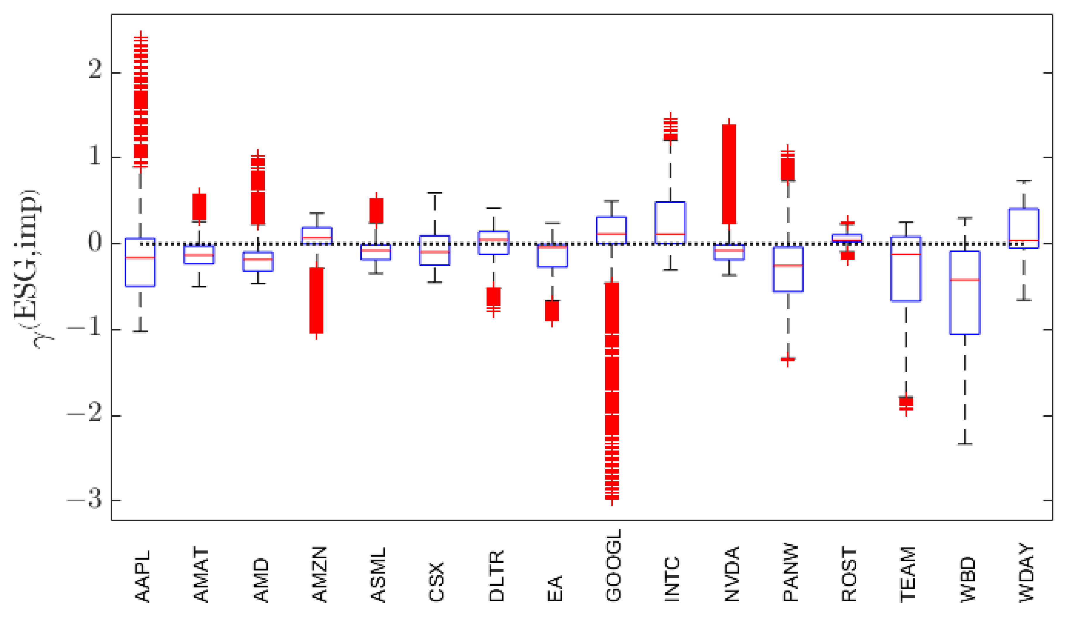
Figure A7 presents the box-whisker summaries of the distributions of values for each of the 16 stocks.
Appendix D. Plots of at(imp)
Figure A8.
The surfaces for which on .
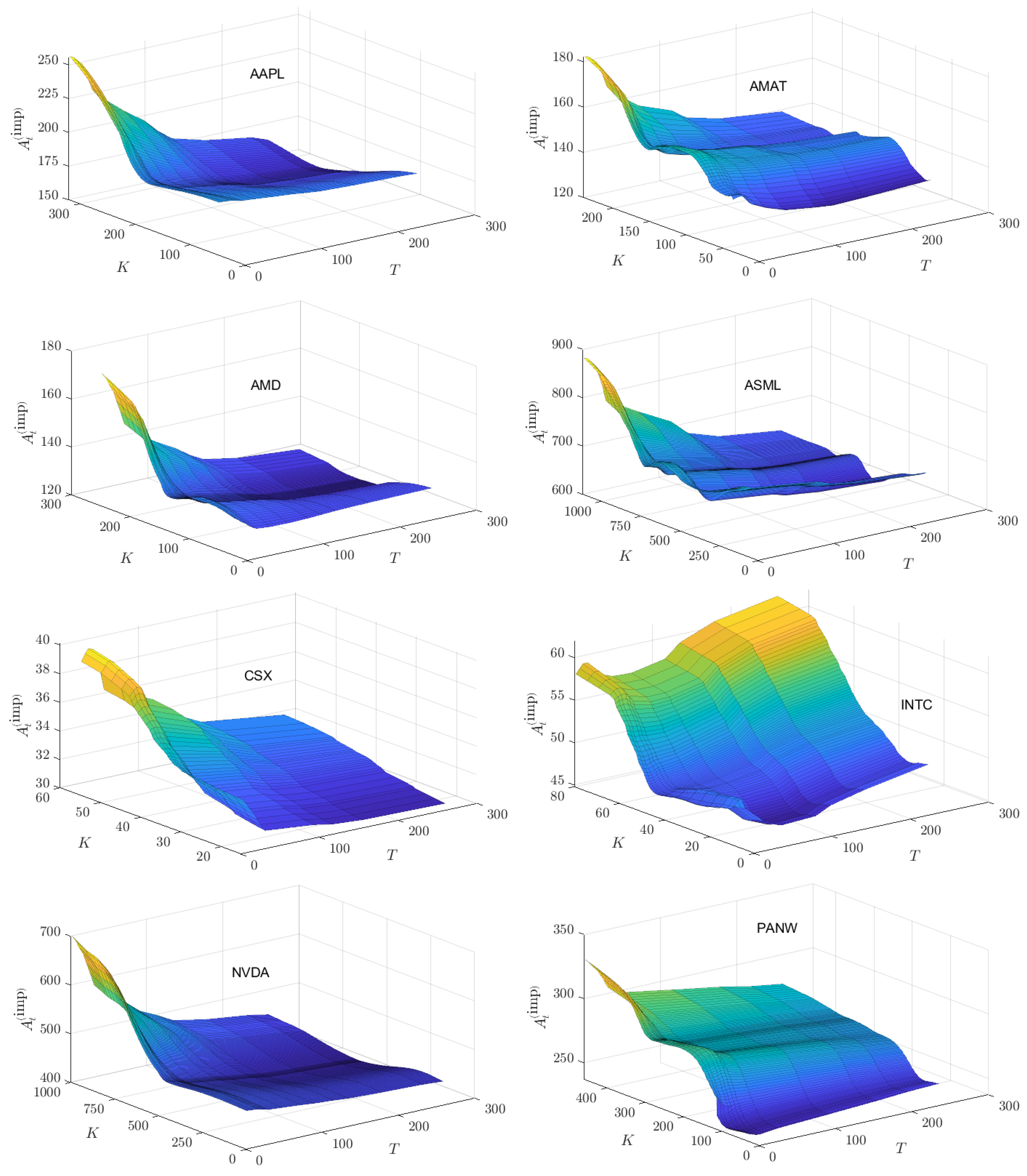
Figure A8 plots as a function of strike price K and time to maturity T for the eight companies for which for , while Figure A9 plots the same for the eight companies for which for
Figure A9.
The surfaces for which on .
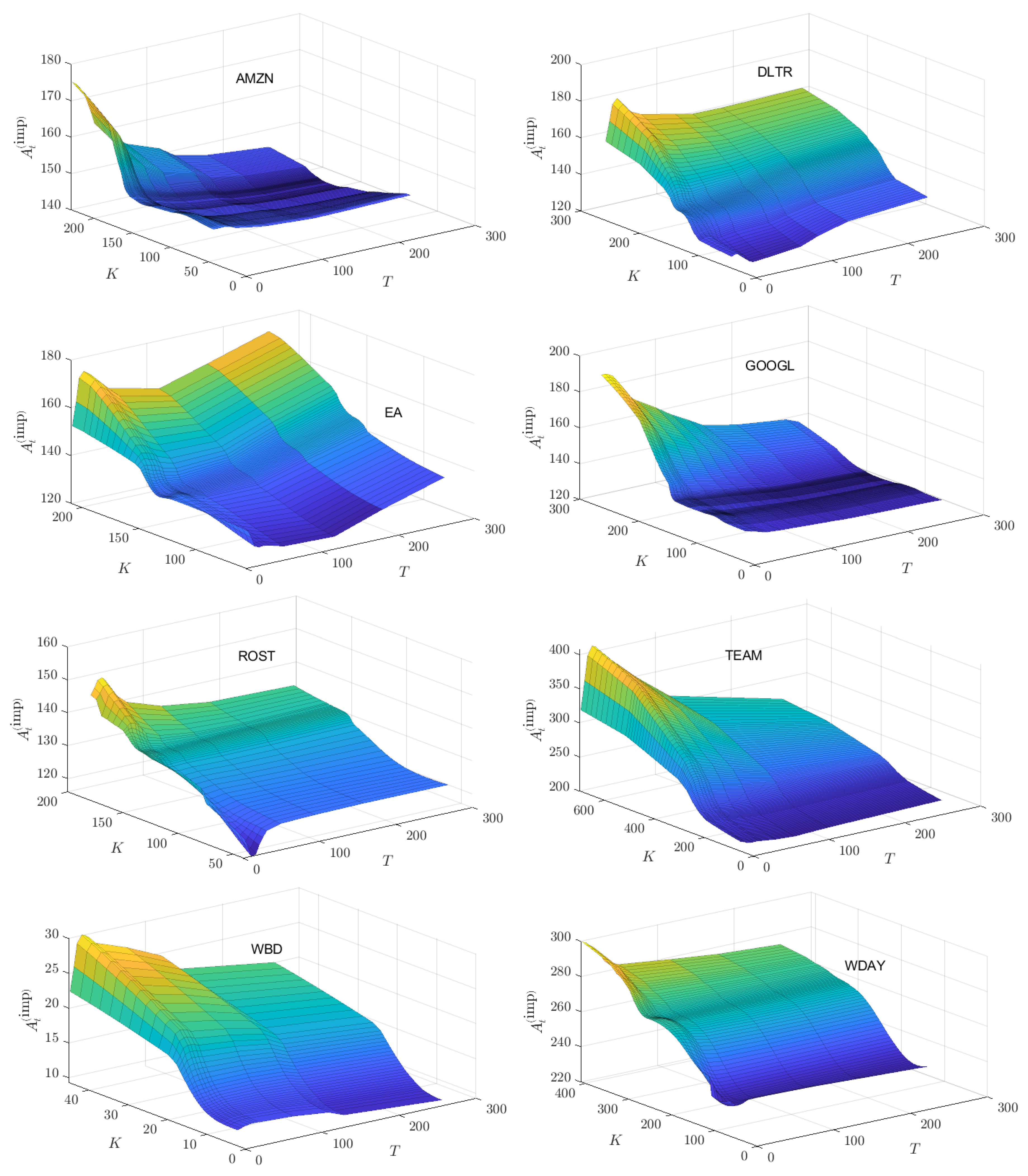
Figure A10.
Contours of for which on .
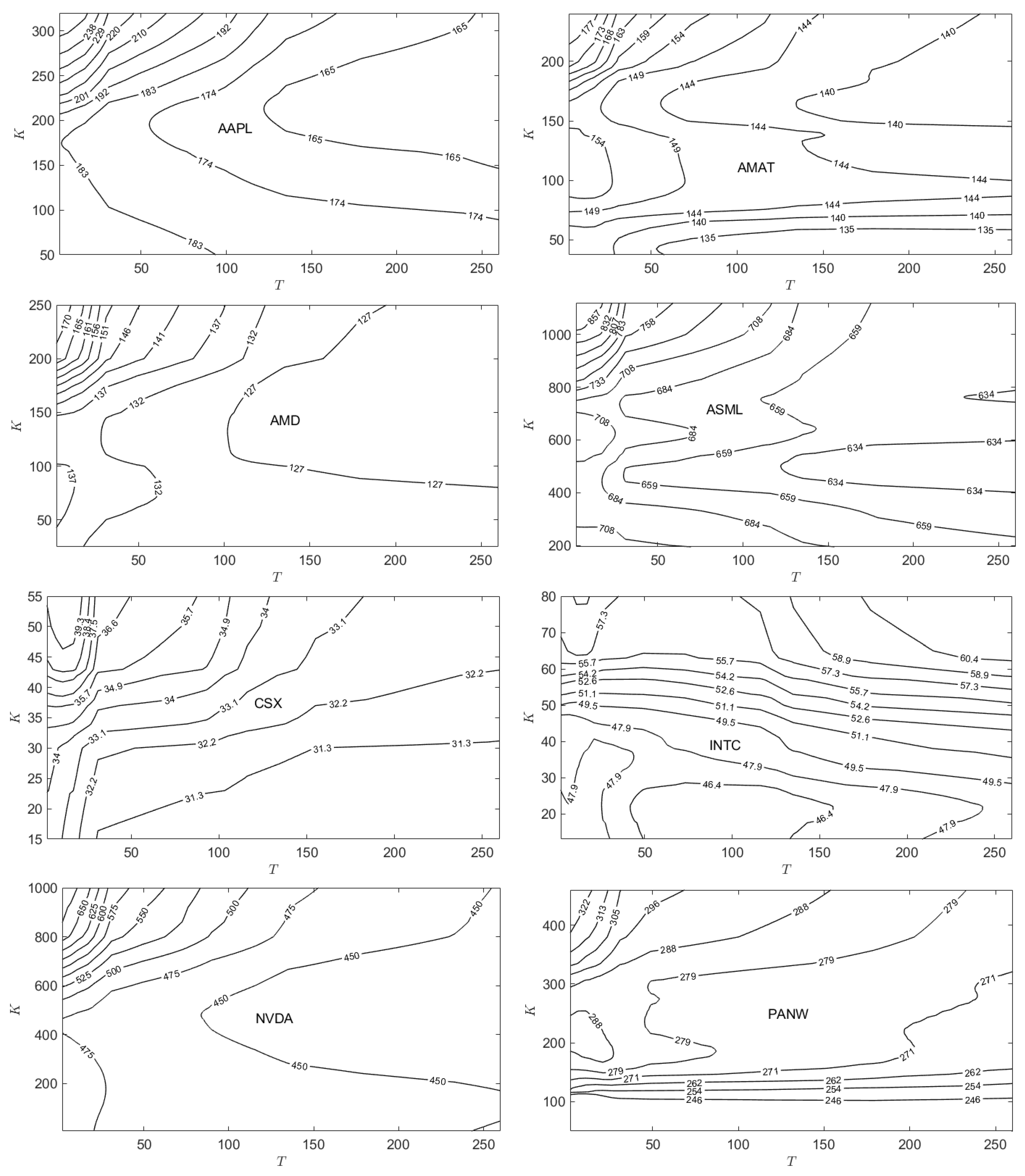
Figure A10 plots contours of as a function of strike price K and time to maturity T for the eight companies for which for while Figure A11 plots the same for the eight companies for which for
Figure A11.
Contours of for which on .
References
- Abu-Mostafa, Yaser and Amir Atiya. 1996. Introduction to financial forecasting. Applied Intelligence 6, 205–213. [CrossRef]
- Alexander, Sidney S. 1961. Price movements in speculative markets: Trends or random walks. Industrial Management Review 2, 7–26.
- Alexander, Sidney S. 1964. Price movements in speculative markets: Trends of random walks, Number 2. Industrial Management Review 5, 25–46.
- Ang, Andrew, William Goetzmann, and Stephen Schaefer. 2010. The efficient market theory and evidence: Implications for active investment management. Foundations and Trends in Finance 5, (3), 157–242. [CrossRef]
- Asare Nyarko, Nancy, Bhathiya Divelgama, Jagdish Gnawali, Blessing Omotade, Svetlozar T Rachev, and Peter Yegon. 2023. Exploring dynamic asset pricing within Bachelier’s market model. Journal of Risk and Financial Management 16, (8), 352. [CrossRef]
- Bachelier, Louis. 1900. Théorie de la spéculation. Annales Scientifiques de l’Ecole Normale Supérieure 3, (17), 21–86.
- Black, Fischer and Myron Scholes. 1973. The pricing of options and corporate liabilities. Journal of Political Economy 81, 637–654. [CrossRef]
- Campbell, John and Samuel Thomson. 2008. Predicting the equity premium out of sample: Can anything beat the historical average? The Review of Financial Studies 21, 1509–1531. [CrossRef]
- Cervelló-Royo, Roberto, Francisco Guijarro, and Kristian Michniuk. 2015. Stock market trading rule based on pattern recognition and technical analysis: Forecasting the DJIA index with intraday data. Expert Systems with Applications 42, 5963–5975. [CrossRef]
- Chakravarty, Sugato, Huseyin Gulen, and Stewart Mayhew. 2004. Informed trading in stock and option markets. The Journal of Finance 59, 1235–1257. [CrossRef]
- Chong, Edwin, Han Chulwoo, and Colin Frank. 2017. Deep learning networks for stock market analysis and prediction: Methodology, data representations, and case studies. Expert Systems with Applications 83, 187–205. [CrossRef]
- Chung, Jaehun and Yongmiao Hong. 2014. Are the directions of stock price changes predictable? A generalized cross-spectral approach. In Econometric Society 2004 North American Winter Meetings. Econometric Society.
- Collin-Dufresne, Pierre, Vyacheslav Fos, and Dmitry Muravyev. 2021. Informed trading in the stock market and option-price discovery. Journal of Financial and Quantitative Analysis 56, 1945–1984. [CrossRef]
- Cootner, Paul. 1964. The Random Character of Stock Market Prices. Cambridge, M.I.T. Press: Massachusetts.
- Del Mar Miralles-Quiros, Maria, Jose Luis Miralles-Quiros, and Irene Guia Arraiano. 2017. Sustainable development, sustainability leadership and firm valuation: Differences across Europe. Business Strategy and the Environment 26, 1014–1028. [CrossRef]
- Duffie, Darrell. 2001. Dynamic Asset Pricing Theory, Princeton University Press: Princeton, NJ.
- Fama, Eugene. 1965. The behavior of stock market prices. Journal of Business 38, 34–105.
- Fama, Eugene. 1970. Efficient capital markets: A review of theory and empirical work. Journal of Finance 25, 383–417.
- Fama, Eugene. 1991. Efficient capital markets: II. The Journal of Finance 46, 1576–1617. [CrossRef]
- Fama, Eugene. 1995. Random walks in stock market prices. Financial Analysts Journal 51, 75–80. [CrossRef]
- Fulton, Mark, Bruce Kahn, and Camilla Sharples. 2012. Sustainable investing: Establishing long-term value and performance. Available at SSRN.
- Hu, Yuan, Abootaleb Shirvani, Stoyan V Stoyanov, Young Shin Kim, Frank J Fabozzi, and Svetlozar T Rachev. 2020. Option pricing in markets with informed traders. International Journal of Theoretical and Applied Finance 23, (06). [CrossRef]
- Jensen, Michael. 1978. Some anomalous evidence regarding market efficiency. Journal of Financial Economics 6, (2/3), 95–101. [CrossRef]
- Leung, Mark, Hazem Daouk, and An-Sing Chen. 2000. Forecasting stock indices: A comparison of classification and level estimation models. International Journal of Forecasting 16, 173–190. [CrossRef]
- Lindquist, W Brent, Svetlozar T Rachev, Jagdish Gnawali, and Frank J Fabozzi. 2024. Dynamic asset pricing in a unified Bachelier–Black–Scholes–Merton model. Risks 12, 375. [CrossRef]
- Malkiel, Burton. 2003. The efficient market hypothesis and its critics. Journal of Economic Perspectives 17, 59–82. [CrossRef]
- Merton, Robert. 1973. Theory of rational option pricing. Bell Journal of Economics and Management Science 4, 141–183.
- Naseer, Muhammad and Tehseen Yasir. 2014. The efficient market hypothesis: A critical review of the literature. IUP Journal of Financial Risk Management 12, 48–63.
- Osborne, Michael. 1959. Brownian motion in the stock market. Operations Research 7, 145–173. [CrossRef]
- Qiu, Ming and Yu Song. 2016. Predicting the direction of stock market index movement using an optimized artificial neural network model. PLoS ONE, 11(5), e0155133. [CrossRef]
- Rachev, Svetlozar T, Nancy Asare Nyarko, Blessing Omotade, and Peter Yegon. 2024. Bachelier’s market model for ESG asset pricing. Journal of Risk and Financial Management 17, (12), 553. [CrossRef]
- Rioul, Olivier. 2018. This is IT: A primer on Shannon’s entropy and information. L’Information, Séminaire Poincaré 23, 43–77. [CrossRef]
- Robinson, David. 2008. Entropy and uncertainty. Entropy 10, 493–506. [CrossRef]
- Rubén, Alberto, Javier García, Francisco Guijarro, and Antonio Peris. 2017. A dynamic trading rule based on filtered flag pattern recognition for stock market price forecasting. Expert Systems with Applications 81, 177–192. [CrossRef]
- Shah, Dev, Haruna Isah, and Farhana Zulkernine. 2019. Stock market analysis: A review and taxonomy of prediction techniques. International Journal of Financial Studies 7, 26. [CrossRef]
- Shiller, Robert J. 2003. From efficient markets theory to behavioral finance. Journal of Economic Perspectives 17, 83–104. [CrossRef]
- Turkington, Joshua and David Walsh. 2000. Informed traders and their market preference: Empirical evidence from prices and volumes of options and stock. Pacific-Basin Finance Journal 8, (5), 559–585. [CrossRef]
- Zhong, Xiao and David Enke. 2017. Forecasting daily stock market return using dimensionality reduction. Expert Systems with Applications 67, 126–139. [CrossRef]
- Zhong, Xiao and David Enke. 2019. Predicting the daily return direction of the stock market using hybrid machine learning algorithms. Financial Innovation 5, (1), 24. [CrossRef]
| 1 | The regularity conditions require that and satisfy the Lipschitz and growth conditions in for [16], Section 5G and Appendix E]. We also require and for all and . To simplify the exposition, we will assume that , , , and have trajectories that are continuous and uniformly bounded on . |
| 2 | Any other choice will result in a riskless asset whose dynamics are inconsistent with that of the risky asset. |
| 3 | The regularity conditions require that satisfies the Lipschitz and growth conditions in for . We also require for all and . To simplify the exposition, we will assume that and have trajectories that are continuous and uniformly bounded on . |
| 4 | Typically the scores are on a zero-to-ten or a zero-to-one-hundred scale. Our data provider, Bloomberg Professional Services, uses the zero-to-ten scale. |
| 5 | The amount of effort to raise an ESG score from 0 to 0.5 is trivial compared to the effort required to raise a score from 9.5 to 10.0. |
| 6 | Under (7), the value of is independent of the range of the scale as long as the range is finite and the same range is used for both and . |
| 7 | In our view, the relative ESG score (which like return and risk-measure is dimensionless), adds a third dimension to conventional risk – return analyses of dynamic asset prices. |
| 8 | As noted in [31], footnote 6, the ESG affinity is expected to change slowly with time. Here we assume it is constant over the both the historical window of prices and the option price maturity times considered. |
| 9 | Hence [31] argued that the MB model, rather than BSM, is better designed to capture the trajectories of ESG-adjusted prices. |
| 10 | In agreement with [22]. |
| 11 | None-the-less, these constant errors propagate multiplicatively along the tree. |
| 12 | The stocks were chosen to represent the full range of ESG scores. |
| 13 | Accessed 01/02/2024. |
| 14 | “Fiscal year scores are provided for a given company once complete ESG data for a specific fiscal year is published.” Source: Bloomberg ESG Scores: Overview & FAQ. https://hr.bloombergadria.com/data/files/Pitanja%20i%20odgovori%20o%20Bloomberg%20ESG%20Scoreu.pdf Accessed 12/22/2024. |
| 15 | Source https://www.slickcharts.com/nasdaq100. Accessed 01/02/2024. |
| 16 | This does not imply an assumption that is not a semi-martingale if falls outside of the range . |
| 17 | The date 01/02/2024 (i.e. ) corresponds to the date for which option price data was collected and used in Section 5 to compute implied ESG affinity values. |
| 18 | |
| 19 | |
| 20 | |
| 21 | Source: Yahoo Finance. Accessed 01/02/2024. |
| 22 | In all plots, the maturity times T are presented in terms of trading days post 01/02/2024. |
| 23 | In preparing the final surface shown, triangulation-based nearest neighbor interpolation was used to fill in missing values in the surface. The surface was then smoothed using a Gaussian weighted, moving average algorithm. This smoothing produced relatively minor changes. |
| 24 | This results in some corresponding surface irregularity (even after smoothing) in the surface. |
| 25 | |
| 26 | The opposite party to this transaction is a noisy trader. |
| 27 | An optimal value for is determined below. |
| 28 | It is sufficient to require terms of to vanish in order to apply invariance principles, such as that by Donsker and Prokhorov, to obtain the continuum limits of this discrete formulation. |
| 29 | Expressed differently, when or , the price movement becomes obvious to all traders and ℵ can therefore be “no more informed” than a noisy trader. |
Figure 1.
Time and level notation for the price evolution of the risky asset on the BBSM binomial tree.
Figure 1.
Time and level notation for the price evolution of the risky asset on the BBSM binomial tree.
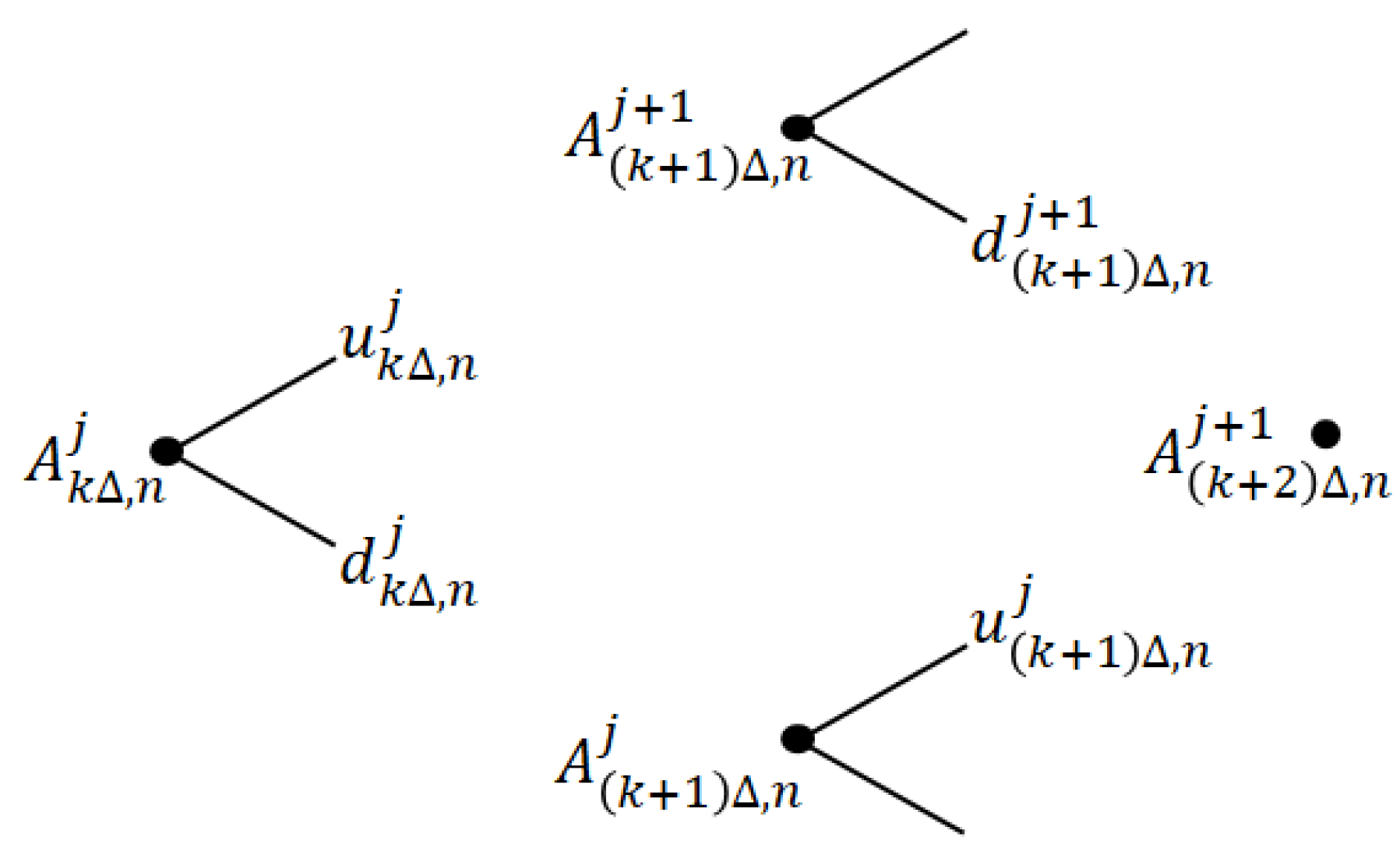
Figure 2.
The relative ESG scores of the 16 chosen companies.
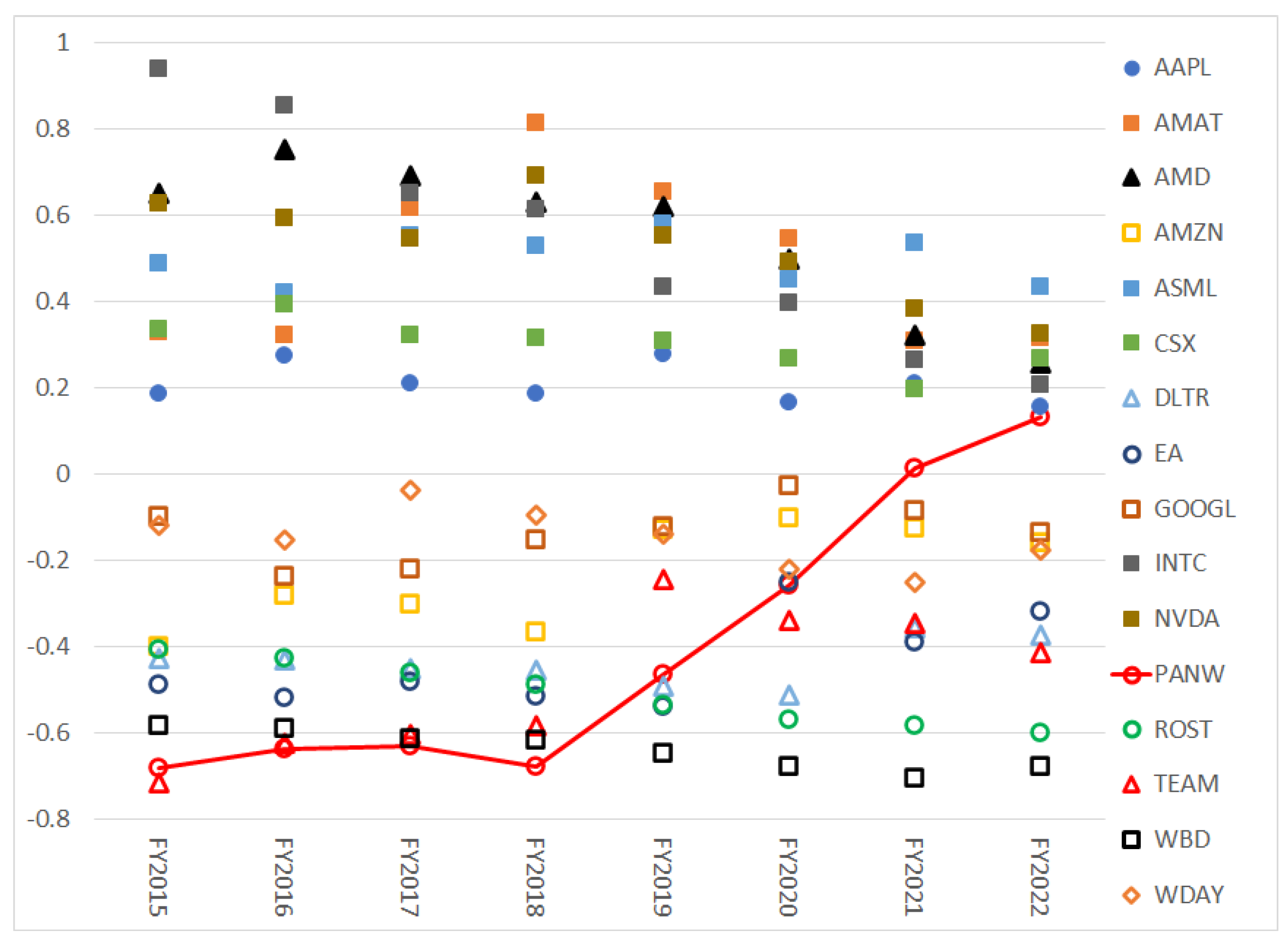
Figure 3.
Illustration of the two-step smoothing process for .
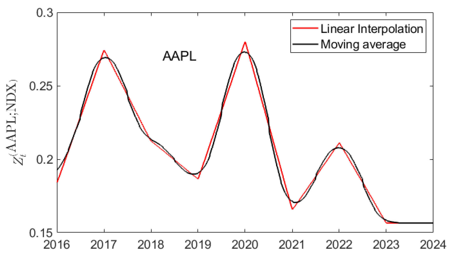
Figure 4.
Signal:noise ratio as a function of .
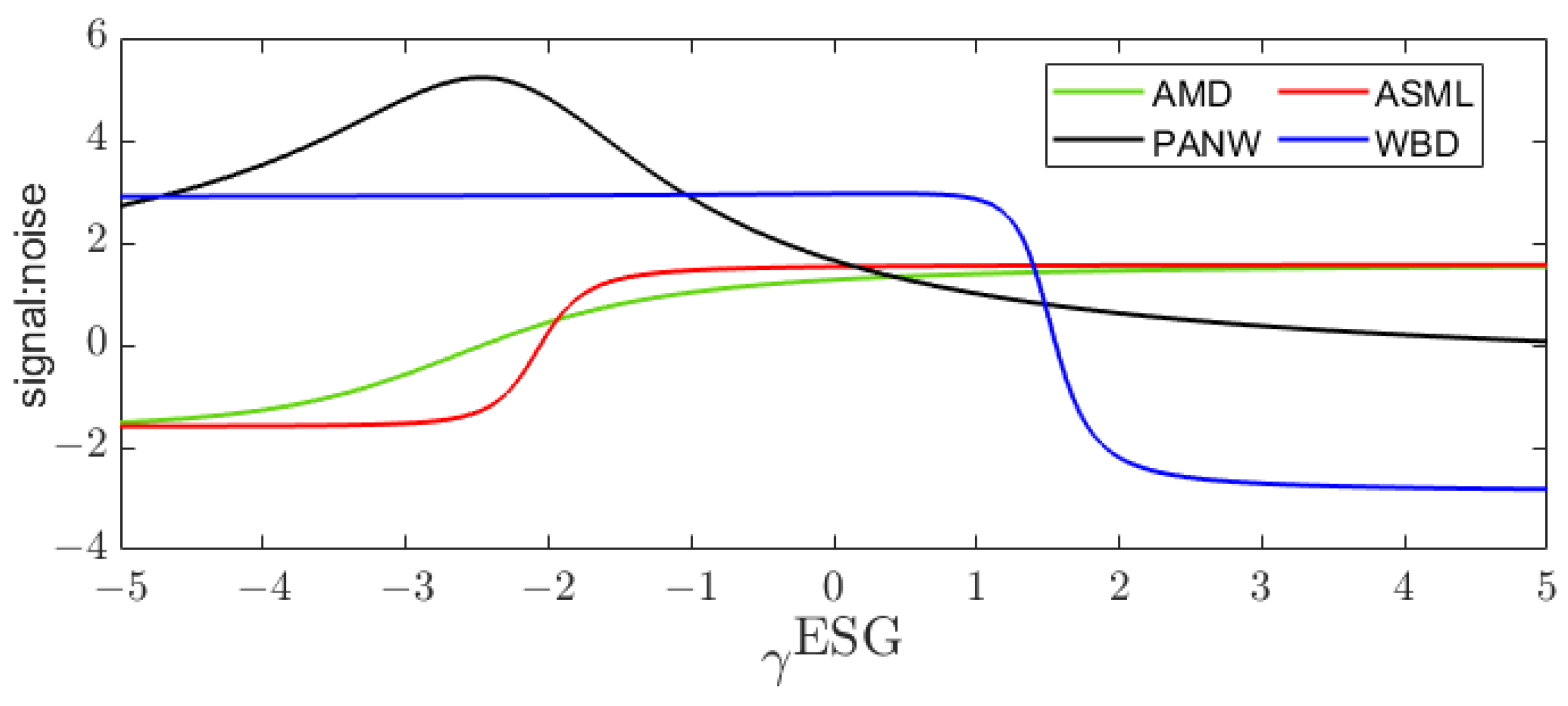
Figure 5.
ESG-adjusted prices of the indicated stocks as is varied over the set of values .
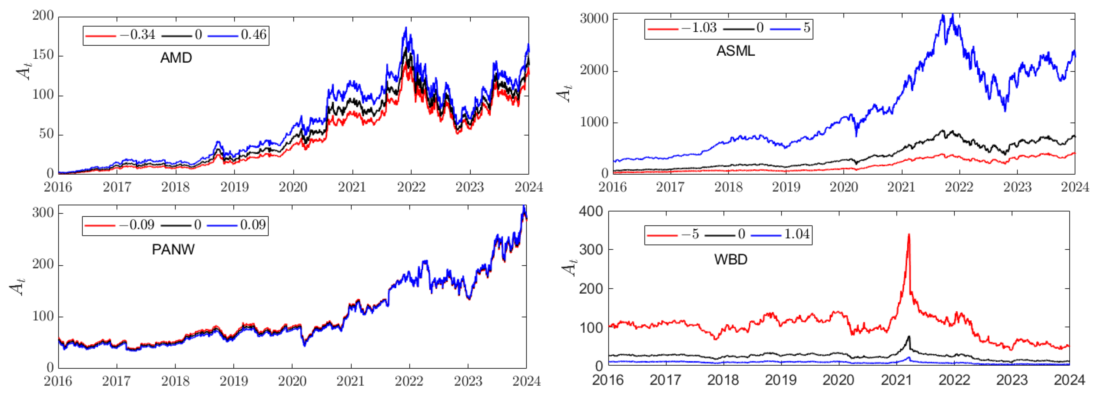
Figure 6.
AMD and ROST parameter dependence on over their respective ranges .
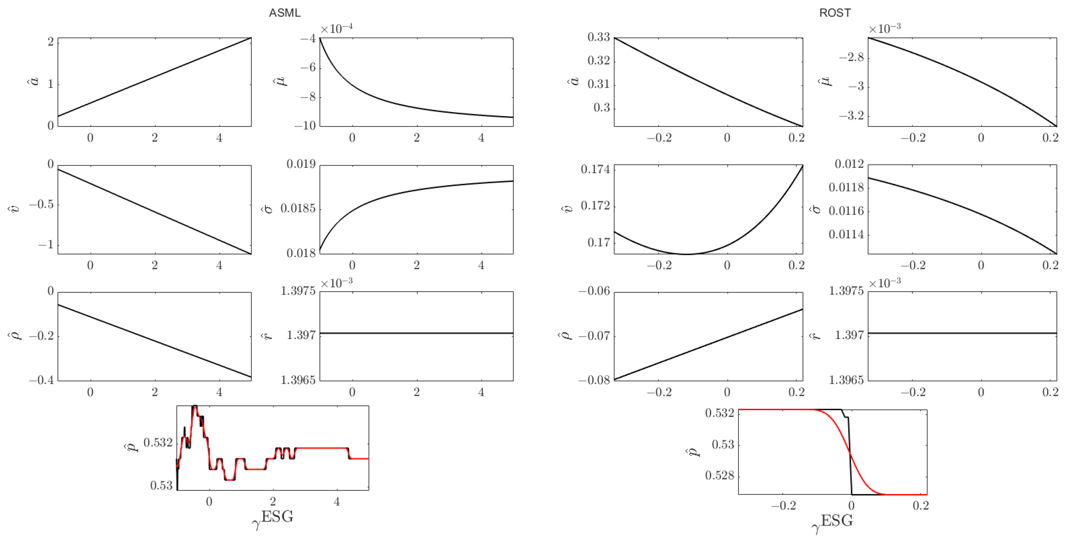
Figure 7.
Range of fitted parameter values, by stock. The upper value of each range is black, the lower value is red. Dotted horizontal lines denote the value 0 or 0.5 as appropriate.
Figure 7.
Range of fitted parameter values, by stock. The upper value of each range is black, the lower value is red. Dotted horizontal lines denote the value 0 or 0.5 as appropriate.
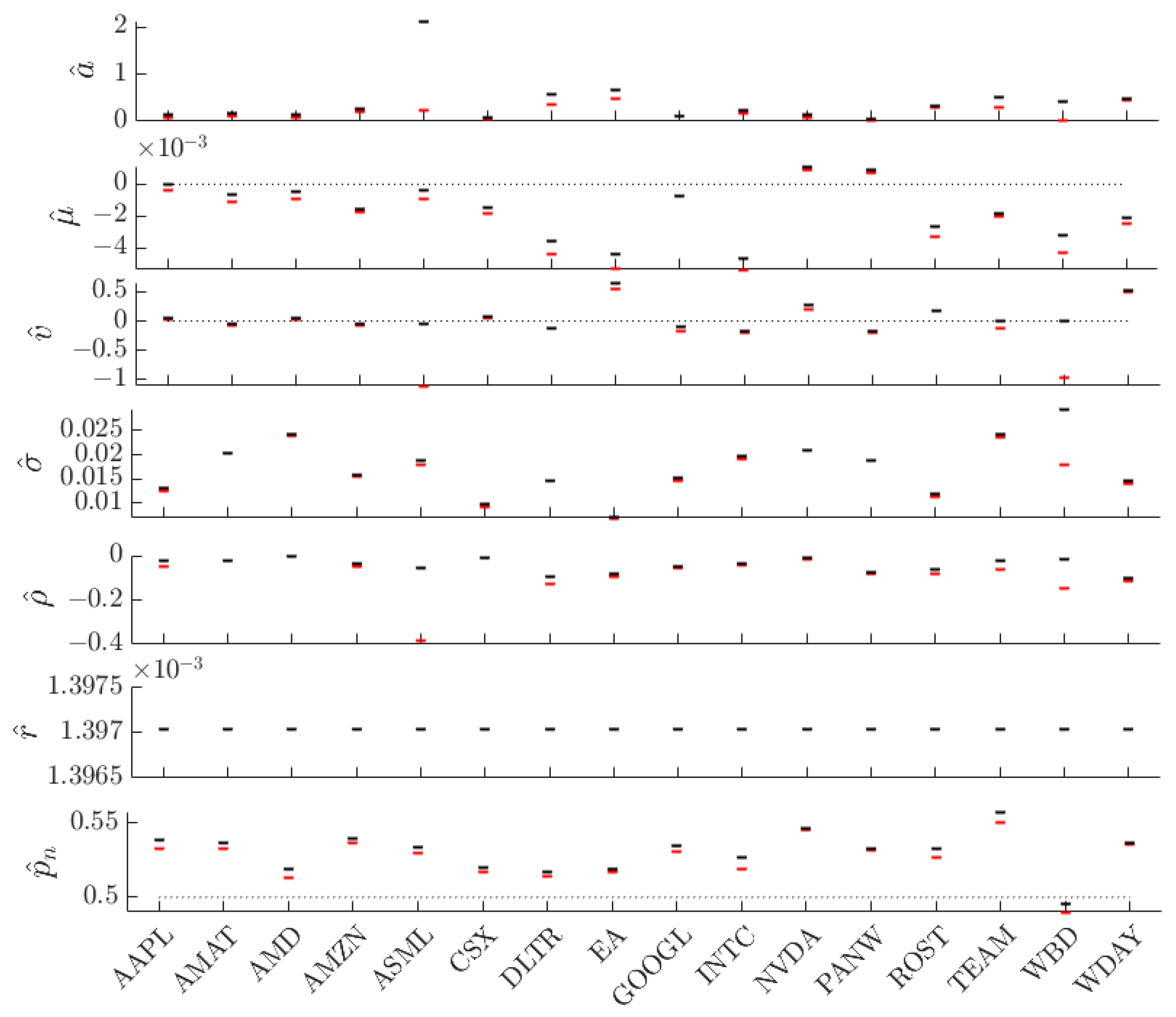
Figure 8.
For the stock AAPL: (top left) The empirical option prices published for AAPL on 01/02/2024. (top right) The computed surface of values. (bottom left) Contours of the surface. (bottom right) Box-whisker summary of the distribution of values.
Figure 8.
For the stock AAPL: (top left) The empirical option prices published for AAPL on 01/02/2024. (top right) The computed surface of values. (bottom left) Contours of the surface. (bottom right) Box-whisker summary of the distribution of values.
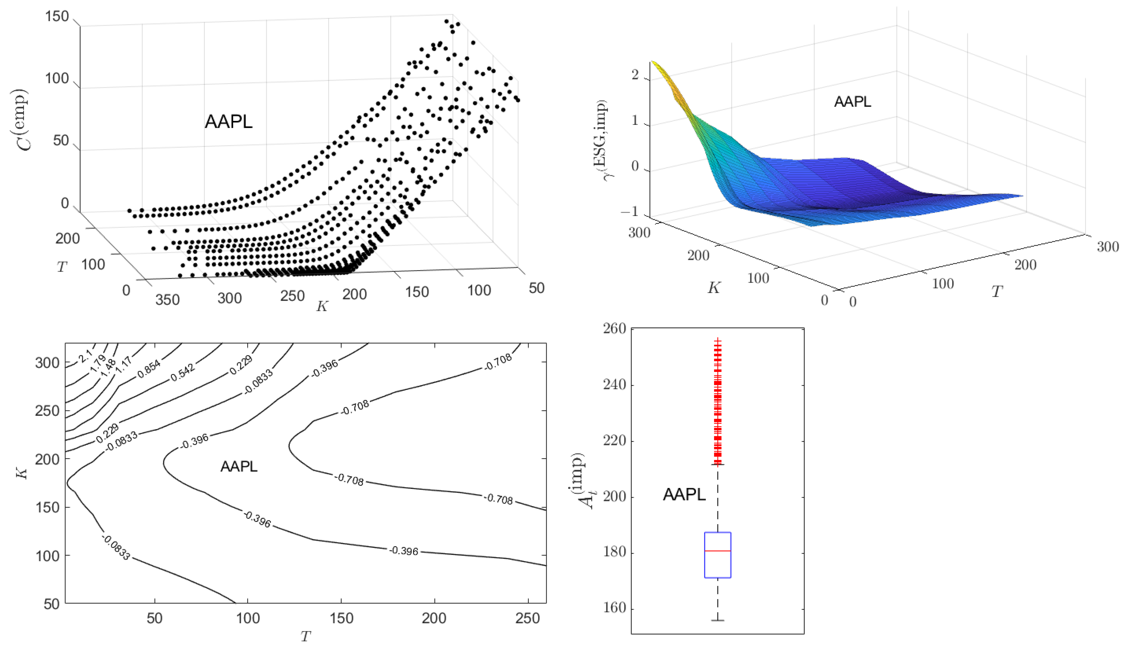
Figure 9.
For the stock AAPL: (left) The computed surface of values. (right) Contours of the surface.
Figure 9.
For the stock AAPL: (left) The computed surface of values. (right) Contours of the surface.
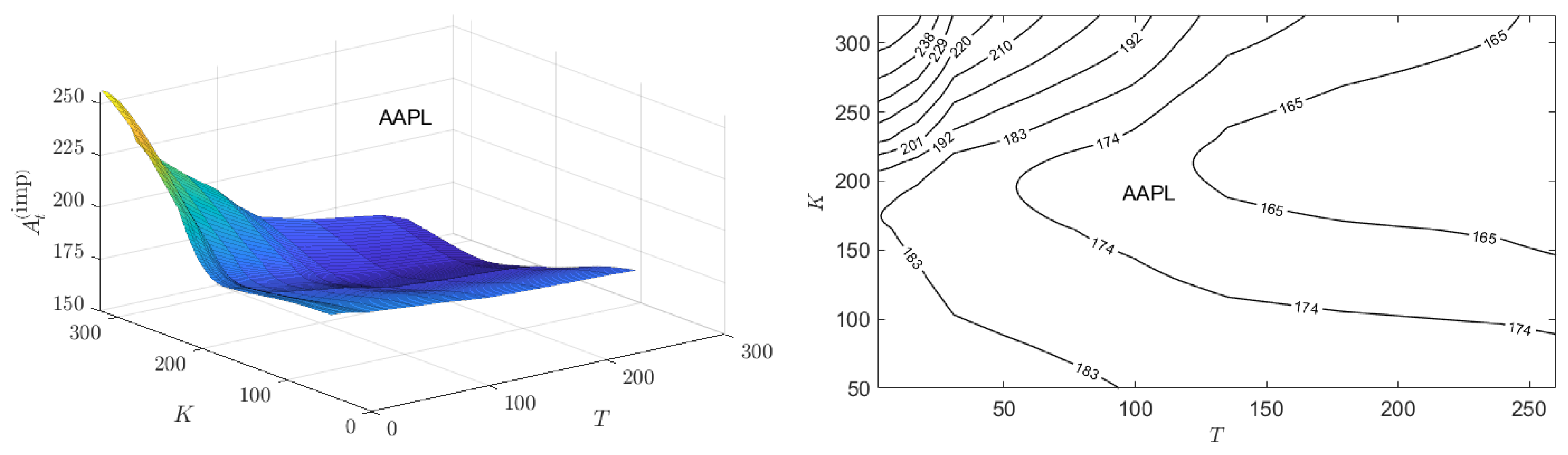
Figure 10.
Box-whisker summaries of the distribution of values for all 16 stocks studied. The “right-arrow” to the left of each box-whisker plot for corresponds to the stock spot price on 01/02/2024.
Figure 10.
Box-whisker summaries of the distribution of values for all 16 stocks studied. The “right-arrow” to the left of each box-whisker plot for corresponds to the stock spot price on 01/02/2024.
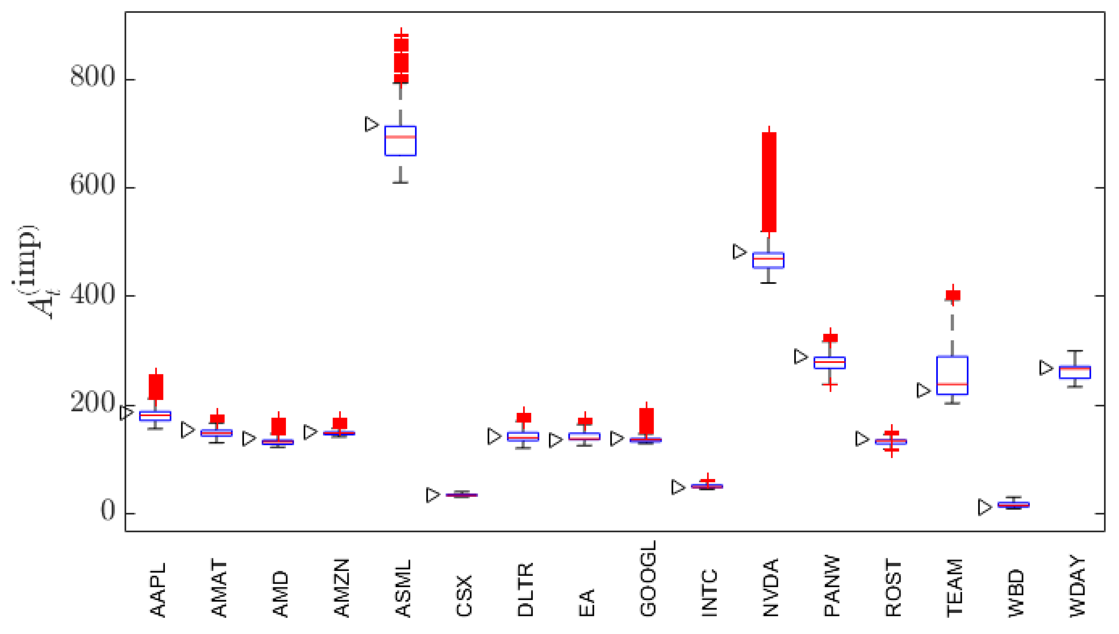
Table 1.
Summaries of the 16 stocks used in the empirical study.
| Ticker | Company Name | GICS Sector | Headquarters |
|---|---|---|---|
| AAPL | Apple Inc. | information technology | Cupertino, CA |
| AMAT | Applied Materials, Inc. | information technology | Santa Clara, CA |
| AMD | Advanced Micro Devices, Inc. | information technology | Santa Clara, CA |
| AMZN | Amazon.com, Inc. | consumer discretionary | Bellevue, WA |
| ASML | ASML Holding NV | information technology | Veldhoven, NL |
| CSX | CSX Corp. | industrials | Jacksonville, FL |
| DLTR | Dollar Tree, Inc. | consumer discretionary | Chesapeake, VA |
| EA | Electronic Arts, Inc. | communication services | Redwood City, CA |
| GOOGL | Alphabet, Inc. | communication services | Mountain View, CA |
| INTC | Intel Corp. | information technology | Santa Clara, CA |
| NVDA | Nvidia Corp. | information technology | Santa Clara, CA |
| PANW | Palo Alto Networks, Inc. | information technology | Santa Clara, CA |
| ROST | Ross Stores, Inc. | consumer discretionary | Dublin, CA |
| TEAM | Atlassian Corp. | information technology | Sydney, AU |
| WDAY | Workday, Inc. | information technology | Pleasanton, CA |
| WBD | Warner Bros Discovery, Inc. | communication services | New York, NY |
Disclaimer/Publisher’s Note: The statements, opinions and data contained in all publications are solely those of the individual author(s) and contributor(s) and not of MDPI and/or the editor(s). MDPI and/or the editor(s) disclaim responsibility for any injury to people or property resulting from any ideas, methods, instructions or products referred to in the content. |
© 2025 by the authors. Licensee MDPI, Basel, Switzerland. This article is an open access article distributed under the terms and conditions of the Creative Commons Attribution (CC BY) license (http://creativecommons.org/licenses/by/4.0/).
Copyright: This open access article is published under a Creative Commons CC BY 4.0 license, which permit the free download, distribution, and reuse, provided that the author and preprint are cited in any reuse.