1. Introduction
In the modern world, data constitute a rich source of digital information that helps us identify patterns, behaviours, or relationships in various fields through statistical analysis. This analysis allows us to extract useful information for decision-making and contributes to the development of scientific research and innovation in various areas, such as disease detection [
1].
When large databases are available, Big Data techniques can be applied for their processing, allowing efficient extraction of the information contained in the data. The development of the Internet of Things enables the generation of large databases in many applications and fields [
2]. Time series processing has numerous applications, including predicting inventory prices and monetary flows, forecasting traffic in the transportation sector, estimating business revenues in the retail field, as well as making predictions in meteorology, tourism, and medical studies, thus facilitating decision-making [
3].
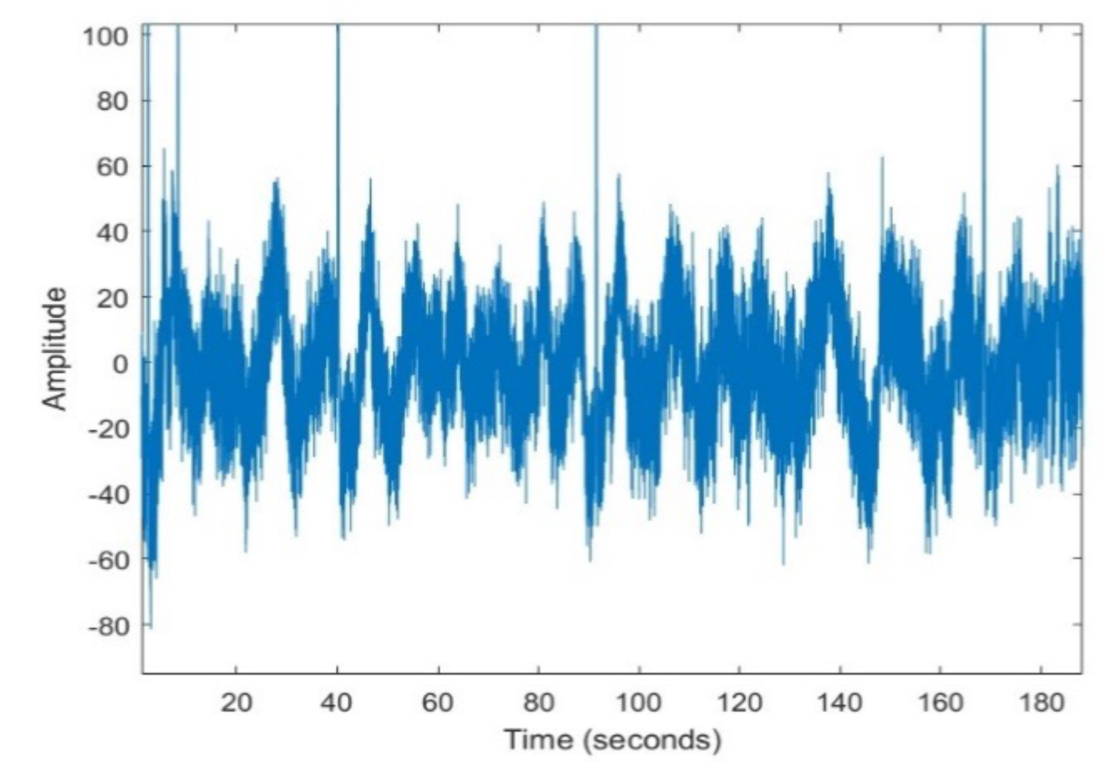
This paper deals with the analysis of electroencephalogram (EEG) signals. EEG signals, are electrical signals generated by the brain’s neuronal activity and recorded from the scalp, which reflect the collective electrical activity of neurons, primarily from the cerebral cortex. EEG signals can be used to measure and monitor brain function [
4]. EEG has been proposed recently as a source of information to be processed for early detection of Parkinson’s disease [
5,
6,
7].
Parkinson’s disease is a neurological disorder that causes disturbances in body movement, tremors, fatigue, muscle stiffness, and stumbling in movement [
8]. Biomedical data from patients with Parkinson’s disease is scarce, primarily because the affected individuals are typically older, and it is not easy for them to cooperate in undergoing the necessary tests to generate large databases [
9]. EEG signals are examples of time series data, that are gathered and prepared according to a selected chronological order [
10]. An example of EEG signal is depicted in
Figure 1, showing the random nature which makes prediction difficult.
Time series data processing is a major challenge in data science, especially when the series are long, complex, and nonlinear. Discovering hidden patterns in these series requires advanced techniques that combine statistical models and artificial intelligence algorithms [
11]. The philosophy of time series forecasting lies in the ability to estimate the value at a future point in time based on previous observations. Despite the importance of these forecasts, their implementation is characterized by many challenges. The noise and missing values that often accompany time series data can reduce the quality of the data, which negatively affects the accuracy of the forecast. The use of inappropriate forecasting models or insufficient data can also reduce the effectiveness of these forecasts [
12]. Time series can be also processed for classification purposes. In the problem at hand, we are interested in classifying the EEG time series according to the characteristics of the people which produced them. Specifically, we are interested in detecting (binary classification) if the person is affected by Parkinson’s disease or not. Classifiers based on artificial intelligence techniques or statistical methods, especially those based on Deep-Learning, need large amount of data for training and testing. When these data are not available, it has been suggested to generate new synthetic data, demonstrating that training improves when they are used.
Currently, there are a variety of methods for generating synthetic data, which can be classified into two main types: traditional methods and machine learning based techniques. Traditional methods include models such as autoregressive (AR), moving average (MA), autoregressive moving average (ARMA) [
13], and autoregressive integrated moving average (ARIMA) [
14]. While these models are effective, they come with some limitations. Traditional methods require smooth and stationary data, which is not always the case in real-world scenarios where time series data is often turbulent and unstable [
15]. With the rapid advancement of AI technology, researchers have shifted their focus towards using neural networks and deep learning techniques to overcome the challenges faced by traditional models [
16].
One effective tool for this purpose is Long Short-Term Memory (LSTM) [
17] a type of recurrent neural network (RNN) that is highly capable of handling complex temporal data.
LSTM is a powerful tool for time series analysis due to its ability to retain information across long sequences of data. It is widely used in applications that require understanding nonlinear and complex temporal patterns, such as analysing financial and medical data, and generating synthetic data that resembles the original data [
18].
In this paper, we use long-short-term memory (LSTM) networks to model the generation of EEG time series data, highlighting their effectiveness in capturing the complex temporal dependencies inherent in neural signals. The ability of LSTMs to retain and utilize long-term patterns as memory, makes them particularly suitable for dealing with the dynamic and nonlinear properties of EEG data. LSTM-based models can effectively reproduce the complex behaviour of EEG time series, providing promising potential for synthetic data generation and other applications in neurophysiological research.
The paper is organized as follows.
Section 1 contains the introduction to the problem tackled in the paper.
Section 2 reviews the main related works and the main concepts about LSTM models and its application to generate synthetic signals.
Section 3 about methodology, describes the materials and methods used in the research. The results are presented and discussed in
Section 4. Finally,
Section 5 contains the conclusions.
2. Review of Knowledge and Related Works
This study considers the use of electroencephalography data (EEG) for training learning machines used to implement diagnosis of major depressive disorders (MDD). The lack of data for effective training has motivated the generation of synthetic data, being [
18] a good example in this way, where Generative Adversarial Networks (GAN) where used. The generated synthetic data where then used to retrain Convolutional Neural Networks (CNN) based detectors, and the results were compared with the results obtained with the baseline detectors.
The synthetic generation of data is also known as “data augmentation”. In [
19], several data augmentation techniques were compared. The research compared 13 different methods for generating synthetic data on two tasks: sleep stage classification and motor imagination classification, in the context of brain-computer interfaces (BCI). The methods used to generate synthetic data included various operations on EEG signals in the temporal, frequency and spatial domains. Two EEG datasets were used for the two different tasks with different predictive models. The results showed that using the appropriate method, the classification accuracy may increase by up to 45%, compared to the results obtained with the same model trained without any augmentation. The procedure was carried out through the use of an open-source Python library known as “scikit-learn” to generate and test data.
An important problem in the generation of synthetic data in EEG applications is non-stationarity. This property makes the use of methods based on linear prediction difficult. This problem has been tackled in [
20], where short-time MEG signals were transformed to the frequency domain, and for the dominant frequencies of 8–12 Hz, the time-series representation was obtained. The stationarity and gaussianity of these time-series were tested, and ARMA models were proposed for their description.
Long Short-Term Memory (LSTM) has been used to model volatile and nonlinear behaviour, such as the one observed in EEG signals. Another example of signals with this behaviour is stock market data. LSTM has been used to predict stock market data in [
21]. Single layer and multilayer LSTM models were developed, and compared using the Root Mean Square Error (RMSE), Mean Absolute Percentage Error (MAPE), and Correlation Coefficient (R), resulting that the single layer LSTM model provides a better fit and higher prediction accuracy.
LSTM has also been applied to long term energy consumption forecasting to capture periodicity in data. The outcomes demonstrated that the suggested strategy beats out conventional forecasting techniques like ARMA, ARFIMA, and Back-propagation neural networks (BPNN), reducing the RMSE by 54.85%, 64.59%, and 19.7%, respectively. The investigation also demonstrated that, even with fewer secondary variables, the suggested algorithm demonstrates outstanding generalization capabilities [
22].
2.1. LSTM Model
A neural network with an LSTM (Long Short-Term Memory) hidden layer is a type of recurrent neural network (RNN) that is primarily used to process sequential data, such as text, time series, or audio sequences. LSTMs are designed to address the problem of long-term dependencies, which is a significant limitation of traditional RNNs [
23].
LSTMs have a specialized architecture that enables them to retain and propagate information over long sequences, thereby preventing the learning process from being hindered by the vanishing gradient problem [
24]. When a neural network has an LSTM hidden layer, its operation follows these key steps:
The input to the network is sequential, meaning the model receives a sequence of vectors, one per time step. The sequence of inputs is fed into the model, one step at a time.
Instead of using a simple dense layer like traditional neural networks, in LSTM networks, the units of the hidden layer are LSTM cells, which are specifically designed to store and process information more efficiently over time.
After passing through the LSTM layer, the output can be used for various purposes depending on the task. In a classification or regression model (e.g., time series prediction), the last hidden state can be passed to a final dense layer to produce the output.
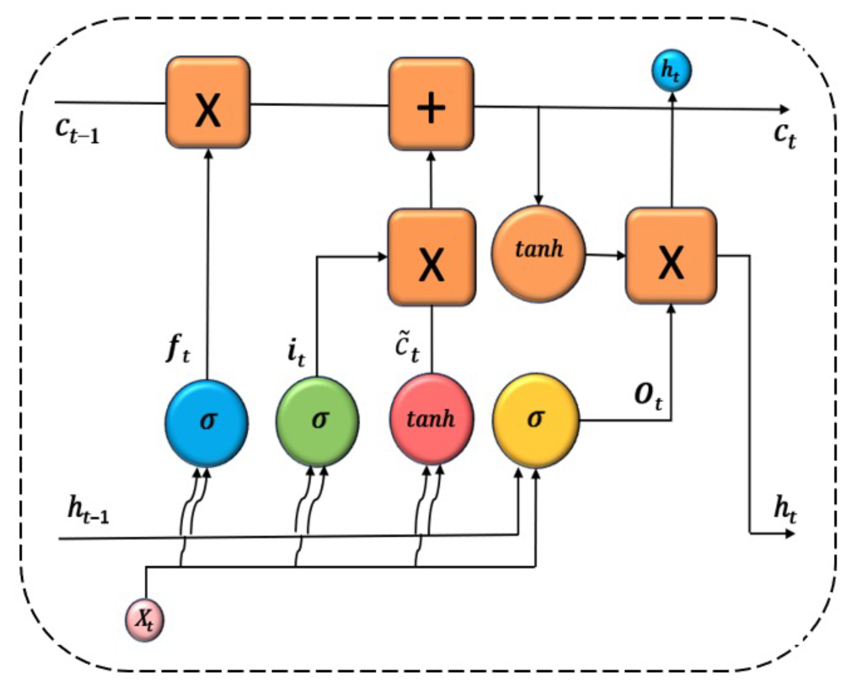
The architecture of the LSTM hidden layer is composed of a series of repeating blocks or cells, which process the information in the input vector, the hidden state, and the cell state. The information processed by the LSTM cell is the following:
Input vector at each time step, .
Hidden state vector, , which represents the current memory of the network. It is initialized to a vector of zeros.
Cell state vector, , with information from the previous cell. It is responsible for storing long-term information over the course of the sequence.
The flow of information through the cell is controlled with three types of gates:
Forget gate, which proceses the previous hidden vector
and the current input
, to produce an output between 0 and 1.
where
is the sigmoid function,
and
are the weights matrixes for the forget gate, and
is a bias vector.
-
Input gate. It takes as input the previous hidden state
and the current input
, and calculates first the relevance of new information
that should be considered for updating the memory:
Being
the concatenation of the previous hidden state and the current input. Additionally, the candidate new information
is calculated:
The input gate controls what part of the new information will update the memory cell:
-
Output gate. It takes the previous hidden state,
, the current input
, and the current cell state
, and outputs a vector of values between 0 and 1, representing how much of the current cell state is used as the current hiddden state
.
The architecture of LSTM can be used for time series forecasting [
24]. The architecture of an LSTM cell is depicted in
Figure 2.
2.2. Bidirectional LSTM (BDLSTM)
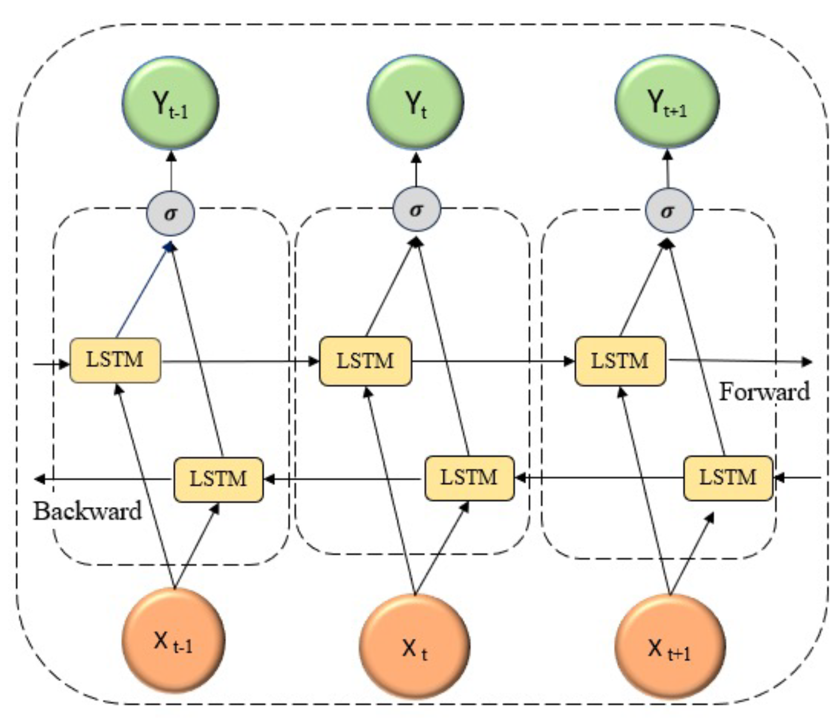
In applications such as analysing EEG (electroencephalography) data for Parkinson’s disease patients, a Bidirectional LSTM (BDLSTM) model can be particularly effective. This model processes time-series data in both directions, making it well-suited to capture complex patterns in the brain signals associated with the disease [
25]. The BDLSTM layer consists of two separate LSTM layers, a forward LSTM layer and a backward LSTM layer:
The Forward Layer processes data in the forward direction, from the beginning to the end of the signal sequence, and its output is iteratively calculated based on positive ordered inputs .
The Backward Layer processes data in the reverse direction, and its output is iteratively calculated using the reversed ordered inputs from time step T to time step 1, .
The output of the BDLSTM layer is finally calculated with expression (
7), where ⊕ refers to the average of the forward and backward predictions.
This design enables the model to access both past and future EEG signals at any given time point, allowing for a deeper analysis of Parkinson’s-related patterns that may not be detectable when relying solely on past signals. The most commonly used loss function for forecasting (sequence prediction) is the Mean Squared Error:
where:
n: number of data samples.
is the current predicted output.
is the model prediction.
3. Methodology
This section includes the description of the dataset used in the experimental work, the way data are pre-processed, and the main parameters of training.
3.1. Dataset
The data used in this study are the UC San Diego Resting State EEG Data from Patients with Parkinson’s Disease, collected at the University of San Diego and curated by Alex Rockhill at the University of Oregon [
26]. The data were obtained using a 40-channel EEG sensor system to capture brain activity signals from 31 individuals, categorized into healthy individuals, patients with Parkinson’s disease without treatment (denoted as "off").
3.2. Preprocessing
The original data were filtered using a bandpass filter with low and high cutoff frequencies of 0.5 Hz and 50 Hz, respectively, to remove noise, as most relevant brain activity falls within the 0.5 Hz to 40 Hz range. Signals collected by the sensors outside this bandwidth are generated by other sources, such as the heart and muscles, which can obscure brain signals, making detection more difficult.
After that, the data are normalized to ensure the dynamic range is consistent across all cases and to avoid any dependence of the results on the acquisition system’s gain. Normalization is implemented using expression (
9), where
and
represent the maximum and minimum signal amplitude values, respectively. Following normalization, the amplitude values fall within the range
. This interval was chosen because the original data contain both positive and negative values.
3.3. Training
The main objective is to use a LSTM neural network to predict samples of EEG signals. The model is trained to minimize the MSE between the original and the synthetic signal, generated with the LSTM neural network.
A neural network based on BDLSTM cells is used, because it allows to learn from patterns in both directions across the time series. This approach enhances the model’s ability to understand temporal relationships by analysing the temporal contexts before. The number of epochs used for training vary from 24 to 50, depending on the person and the channel that is considered.
The number of BDLSTM cells in the model has been determined empirically, by evaluating the model with increasing number of cells in the hidden layer, and measuring the MSE between the original and the synthetic signal, and the Pearson’s correlation coefficient.
The main parameters used during training are the following:
The cost or error function used for training is the Mean Square Error (MSE).
The model was trained with the Back Propagation (BP) algorithm. The learning rate for the BP algorithm was set to .
The training dataset was split into two subsets, one with 98% of the available data used for training, and the remining 2% were used for testing.
We have used a Dropout layer, which is useful to reduce high data flow within a neural network and to prevent overfitting. When the dropout rate is fit to 0.2, during each training step, 20% of the neurons are randomly dropped. This reduces the data load flowing through the network and enhances the model’s ability to generalize, leading to better performance on new data.
We also used the Hyperbolic Tangent (Tanh) activation function, which is a commonly used activation function in neural networks, especially in hidden layers. The Tanh function is specially useful if we have values ranging from to 1.
4. Experiments and Results
Several experiments have been carried out to decide which is the best structure based on BDLSTM cells to predict the EEG signals.
4.1. Number of Cells of the BDLSTM Neural Network
The BDLSTM basic model has been trained and tested with an increasing number of cells (hidden units) in the hidden layer. The prediction MSE and the correlation between the synthetic and the original signal have been measured with the testing dataset, for all the people in the dataset. The MSE decreases until the number of hidden units is around ten in all cases. At the same time, the correlation between the synthetic and original signals increases, with an asymptotic behaviour too.
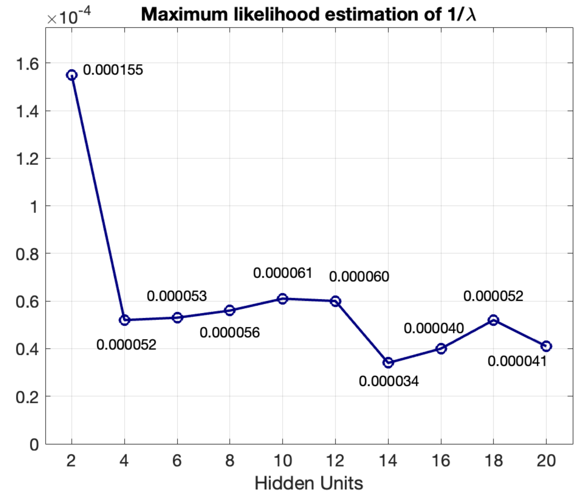
Additionally, we have studied the statistical distribution of the MSE estimations for a given number of hidden units. We have discovered that the MSE estimation distribution fits well to the exponential distribution, and the parameter of this distribution can be estimated with the Maximum Likelihood estimator:
Figure 4 represents the variation of the inverse of the estimated parameter of the exponential probability density function (
), corresponding to channel F7 of a group of 31 people in the dataset (with Parkinson’s disease without taking medicine, and healthy people). As lower the value of
, lower the MSE, and better the results of signal estimation.
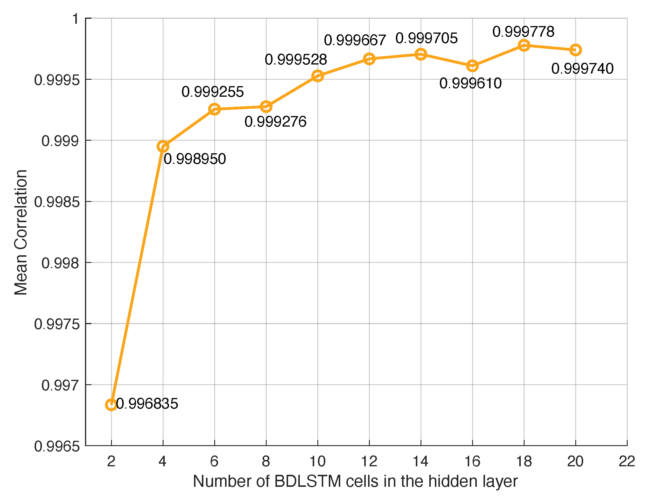
Figure 5 depicts the mean correlation coefficient between the signal corresponding to channel 7 of the group of 31 people in the database, and its prediction with the BDLSTM based neural network. It has an asymptotic behaviour, reaching to a flat zone when the number of BDLSTM cells is 10.
The best results studying the MSE are obtained when the number of hidden units is 14. When the mean of the correlation coefficient is studied, very good results are obtained, even with very low number of units in the hidden layer. Nevertheless, the correlation is especially high when the number of cells in the hidden unit is higher than 12, with very low differences. Therefore, 14 units have been chosen, which combines the best results in MSE and correlation coefficient.
4.2. Length of the Hidden State Vector
The length of the hidden state vector is the number of previous samples in the time series used to predict the current sample. The optimum length has been determined experimentally by measuring the MSE and correlation when this length changes. In the experiment, we have used the number of hidden cells obtained previously (14 hidden units in the hidden layers).
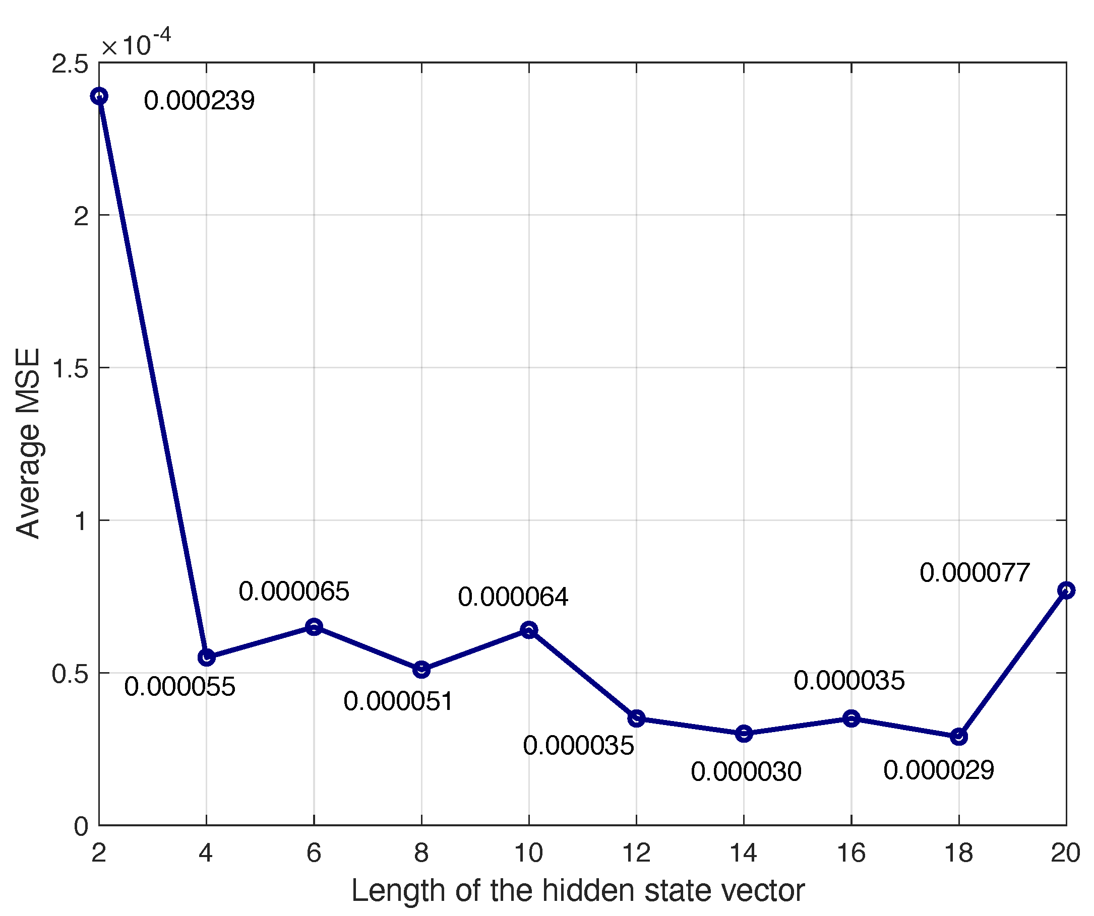
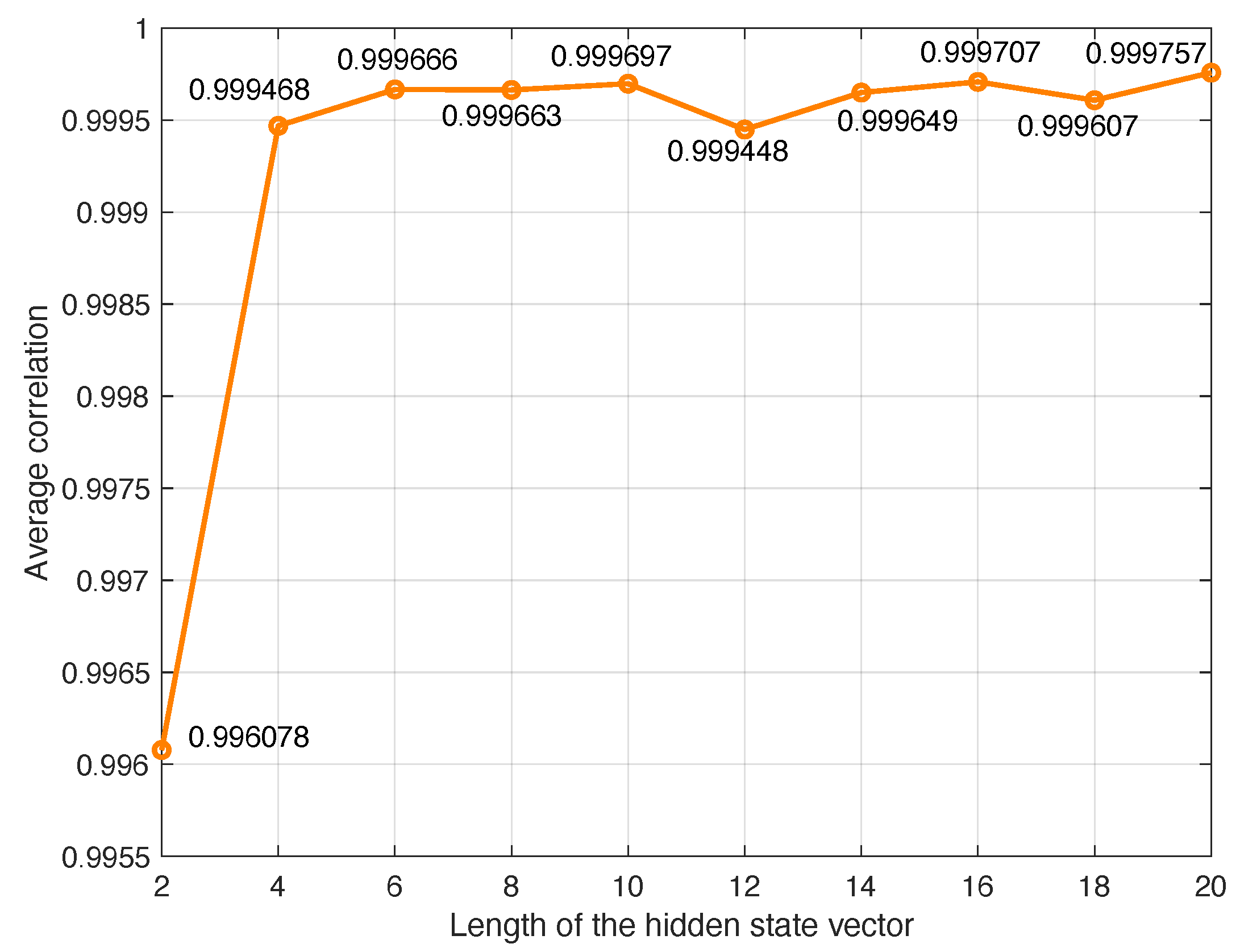
Figure 6 and
Figure 7 represent the average MSE and correlation obtained when increasing the length of
. It is observed that the mean MSE arrieves to a reduced value with length equal 4, and after that, a slight reduction is obtained when the length increases, which do not compensate the higher resources used in the implementation. The correlation also arrives to a very good value with length equal 4. Therefore, this value has been chosen in the model to generate synthetic EEG signals.
5. Conclusions
This research has contributed to the design of models useful to generate synthetic signals from real measurements. We have used the BDLSTM model, optimising the number of hidden units of the cells, and the length of the hidden state vector. A model has been built for each available signal in a dataset, demonstrating that the result after optimisation is similar will all the available signals.
The optimisation process achieves a good trade-off between complexity and modelling error, in order to save computational resources when building non-linear models to generate synthetic samples that have the same statistical characteristics than the original signals obtained with measurement.
In the experiments carried out, the original signals are EEG recordings of patients with Parkinson’s disease. The need for synthetic signals comes from the necessity to train deep-learning neural networks to distinguish Parkinson’s disease patients from healthy people. For training hidden neural networks, with a huge number of parameters, many training samples are needed, to avoid overfitting. Large datasets are not usually available, and data augmentation appears as the solution to this problem. The models built in this paper will be used to generate synthetic signals as the way to increase the size of the training dataset, following the strategy of data augmentation.
Therefore, the practical value of this study lies in its ability to offer innovative solutions to the problem of data scarcity, a challenge that impacts many research fields, particularly in medicine, where collecting data from disease patients is a complex and costly process. This methodology allows for the generation of reliable synthetic datasets that can be used in analysis and development without the need for additional data sources.
The significance of this study extends beyond the medical field; it provides groundbreaking tools that could be applied in a wide range of disciplines, from engineering sciences to financial analysis. Via leveraging this technology, researchers can simulate accurate data that contributes to a deeper understanding of natural, economic, and social phenomena, paving the way for new scientific discoveries, fostering innovation, and tackling research challenges in ways that were previously unattainable.
Author Contributions
Conceptualization and methodology, Manuel Rosa-Zurera and Bakr Rashid Alqaysi; software, Bakr Rashid Alqaysi and Ali Abdulameer Aldujaili; validation, Manuel Rosa-Zurera and Bakr Rashid Alqaysi.; formal analysis, Manuel Rosa-Zurera, Bakr Rashid Alqaysi, and Ali Abdulameer; investigation, Manuel Rosa-Zurera, Bakr Rashid Alqaysi, and Ali Abdulameer; resources, Manuel Rosa-Zurera; data curation, Bakr Rashid Alqaysi, and Ali Abdulameer; writing—original draft preparation, Bakr Rashid Alqaysi; writing—review and editing, Manuel Rosa-Zurera and Bakr Rashid Alqaysi; visualization, Manuel Rosa-Zurera and Bakr Rashid Alqaysi; supervision, Manuel Rosa-Zurera; project administration, Manuel Rosa-Zurera; funding acquisition, Manuel Rosa-Zurera. All authors have read and agreed to the published version of the manuscript.
Funding
This research was funded by MCIN/AEI/10.13039/ 501100011033/FEDER, UE with the project PID2021-129043OB-I00.
Conflicts of Interest
The authors declare no conflicts of interest.
Abbreviations
The following abbreviations are used in this manuscript:
| AR |
Autoregressive |
| ARFIMA |
Autoregressive Fractional Integrated Moving Average |
| ARIMA |
Autoregressive integrated Moving Average |
| ARMA |
Autoregressive Moving Average |
| BCI |
brain-computer interfaces |
| BP |
Back Propagation |
| BPNN |
Back-propagation neural networks |
| CNN |
Convolutional Neural Networks |
| EEG |
Electro-Encephalogram |
| GAN |
Generative Adversarial Networks |
| HZ |
Hertz |
| LSTM |
Long Short-Term Memory |
| MA |
Moving Average |
| MAPE |
Mean Absolute Percentage Error |
| MDD |
implement diagnosis of major depressive disorders |
| MEG |
Magnetoencephalography |
| MSE |
Mean-squared error |
| R |
Correlation Coefficient |
| RNN |
recurrent neural network |
| RMSE |
Root Mean Square Error |
| BDLSTM |
Bidirectional Long Short-Term Memory |
References
- Wang, W. Y. C. & Wang, Y. (2020). Analytics in the era of big data: The digital transformations and value creation in industrial marketing. Industrial Marketing Management, 86, 12-15, Elsevier Inc.; [CrossRef]
- Ma, X. & Li, J. & Guo, Z. & Wan, Z. (2024). Role of big data and technological advancements in monitoring and development of smart cities, Heliyon, 10(15), paper number e34821; DOI:10.1016/j.heliyon.2024.e34821.
- Karamanou, A. & Kalampokis, E. & Tarabanis, K. (2022). Linked Open Government Data to Predict and Explain House Prices: The Case of Scottish Statistics Portal, Big Data Research, 30, paper number 100355, . [CrossRef]
- Morales, S.. & Bowers, M.E. (2022). Time-frequency analysis methods and their application in developmental EEG data, Developmental Cognitive Neuroscience, 54, paper number 101067, . [CrossRef]
- Preetha, M. & Rao Budaraju, R. & Aruna Sri, P. S. G. & Padmapriya, T. (2024), Deep Learning-Driven Real-Time Multimodal Healthcare Data Synthesis, International Journal of Intelligent Systems and Applications in Engineering, 12(5S), 360-369;
- Müller-Nedebock, A.C. & et al., (2023), Different pieces of the same puzzle: a multifaceted perspective on the complex biological basis of Parkinson’s disease, NPJ Parkinson’s Disease, 9, Article number: 110; [CrossRef]
- Zhang, R. & Jia, J. & Zhang, R. (2022), EEG analysis of Parkinson’s disease using time–frequency analysis and deep learning, Biomed Signal Processing and Control, 78, Paper number: 103883; [CrossRef]
- Kulcsarova, K. & Skorvanek, M. & Postuma, R. B. & Berg, D. (2024), Defining Parkinson’s Disease: Past and Future, Journal of Parkinson’s Disease, 14(s2), S257-S271; [CrossRef]
- Guillaudeux, M. et al. (2023), Patient-centric synthetic data generation, no reason to risk re-identification in biomedical data analysis, NPJ Digital Medicine, 6, Article number: 37; [CrossRef]
- Choi, K. & Yi, J. & Park, C. & Yoon, S. (2021), Deep Learning for Anomaly Detection in Time-Series Data: Review, Analysis, and Guidelines, IEEE Access, 9, 120043-120065; [CrossRef]
- Blázquez-García, A. & Conde, A. & Mori, U. & Lozano, J. A. (2021), A Review on Outlier/Anomaly Detection in Time Series Data, ACM Computing Surveys, 54(3), Article No.: 56; [CrossRef]
- Iwana, B. K. & Uchida, S. (2021), An empirical survey of data augmentation for time series classification with neural networks, Plos One, 16(7), e0254841; [CrossRef]
- Cebrián, A.C. & Salillas, R. (2021), Forecasting High-Frequency River Level Series Using Double Switching Regression with ARMA Errors, Water Resources Management, 36(1), 299-313; [CrossRef]
- Sánchez-Espigares, J.A. & Acosta Argueta, L.M., Lecture Notes on Forecasting Time Series; Polytechnic University of Catalonia (UPC), Spain, 2024.
- Deng, J. & Chen, X. & Jiang, R. & Song, X. & Tsang, I.W., ST-Norm: Spatial and Temporal Normalization for Multi-variate Time Series Forecasting. In Proceedings of the ACM SIGKDD International Conference on Knowledge Discovery and Data Mining, Aug. 2021; pp. 269–278. [CrossRef]
- Wen, X. & Li, W. (2023), Time Series Prediction Based on LSTM-Attention-LSTM Model, IEEE Access, 11, 48322–48331; [CrossRef]
- Liu, P. (2022), Time Series Forecasting Based on ARIMA and LSTM, In Proceedings of the 2022 2nd International Conference on Enterprise Management and Economic Development (ICEMED 2022), July. 2022; pp. 1203-1208. [CrossRef]
- Carrle, F.P. & Hollenbenders, Y. & Reichenbach, A. (2023), Generation of synthetic EEG data for training algorithms supporting the diagnosis of major depressive disorder, Frontiers in Neuroscience, 17, 1219133; [CrossRef]
- Rommel, C. & Paillard, J. & Moreau, T. & Gramfort, A. (2022), Data augmentation for learning predictive models on EEG: a systematic comparison, Journal of Neural Engineering, 19(6), 066020; [CrossRef]
- Kipiński, L. & Kordecki, W. (2021), Time-series analysis of trial-to-trial variability of MEG power spectrum during rest state, unattended listening, and frequency-modulated tones classification, Journal of Neuroscience Methods, 363, 109318; [CrossRef]
- Bhandari, H. N. & Rimal, B. & Pokhrel, N. R. & Rimal, R. & Dahal, K.R. & Khatri, R.K.C. (2022), Predicting stock market index using LSTM, Machine Learning with Applications, 9, p. 100320; [CrossRef]
- Pyo, J.C. et al. (2023), Long short-term memory models of water quality in inland water environments, Water Research X, 21, p. 100207; [CrossRef]
- Brownlee, J., Long Short-Term Memory Networks with Python: Develop Sequence Prediction Models with Deep Learning, Machine Learning Mastery, 2017.
- Fang, Z. & Ma, X. & Pan, H. & Yang, G. & Arce, G.R., (2023), Movement forecasting of financial time series based on adaptive LSTM-BN network, Expert Systems with Applications, 213(part C), 119207; [CrossRef]
- Liu, Q. et al. (2023), A cloud-based Bi-directional LSTM approach to grid-connected solar PV energy forecasting for multi-energy systems, Sustainable Computing: Informatics and Systems, 40, 100892; [CrossRef]
- Rockhill, A.P. & Jackson, N. & George, J. & Aron, A. & Swann, N.C. (2020). UC San Diego Resting State EEG Data from Patients with Parkinson’s Disease. OpenNeuro. [Dataset] . [CrossRef]
|
Disclaimer/Publisher’s Note: The statements, opinions and data contained in all publications are solely those of the individual author(s) and contributor(s) and not of MDPI and/or the editor(s). MDPI and/or the editor(s) disclaim responsibility for any injury to people or property resulting from any ideas, methods, instructions or products referred to in the content. |
© 2025 by the authors. Licensee MDPI, Basel, Switzerland. This article is an open access article distributed under the terms and conditions of the Creative Commons Attribution (CC BY) license (http://creativecommons.org/licenses/by/4.0/).