
Submitted:
27 January 2025
Posted:
29 January 2025
You are already at the latest version
Abstract
Utilizing the concept of rough upper approximation neighborhood
systems in simple graphs, this paper introduces a novel class of
topologies on vertex sets. We delve into identifying the specific
graphs that induce either the indiscrete or discrete topology,
unraveling essential topological properties within this
classification. Exploring further, we delve into the continuity and
isomorphism of graph mappings. Subsequently, we apply these findings
to enhance radar chart graphical methods through the analysis of
corresponding graph structures.
Keywords:
Simple graph
; approximated G-topology
; neighborhood system
; continuous function
; radar chart
MSC: 05C99; 05C20, 54C10, 54D99
1. Introduction
Two important branches of mathematics, general topology [1] and graph theory [2], are closely related. One of the relationships between graph theory and general topology is constructing topologies on the vertices set and the edges set of a graph. Several studies constructed some topologies via directed graphs and undirected graphs. Most of these constructions were in the theory of simple undirected graphs, in particular on the vertices sets of such graphs. In 2018, the authors of the paper [3], introduced new constructions of topologies, incidence topology on the set of vertices for simple graphs without isolated vertices, which has a subbasis , where is the family of end-sets that contain only end points of each edge. Kiliciman and Abdu [4], used the graphs to introduce two constructions of topologies on the set , called compatible edge topology and incompatible edge topology. Amiri et al. [5] constructed the graphic topological space of a graph as a pair , where is an Alexandroff topology on induced by a subbasis which is the family of open neighbourhoods of vertices in . Nada et al., [6], introduced a relation on graphs to generate new types of topological structures. In 2019, Nianga and Canoy [7], constructed a topology on simple graphs by using unary and binary operations, and in [8], they introduced some topologies on the vertices set in the theory of simple graphs by using the hop neighborhoods of the graphs (see also [9,10]). In 2020, for the simple graphs without isolated vertices , Sari and Kopuzlu [11], generated topology on the vertices set induced by the same basis which is introduced by Amiri et al. [5] and studied the continuity of functions. The minimal neighborhood system of vertices and the discrete property of topologies for special graphs, such as complete graphs , cycle graphs and complete bipartite graphs , are also studied,. In 2021, Zomam et al. [12] studied some conditions for a locally finite property of graphs to get an Alexandroff property for the graphic topological spaces which are introduced by Amiri et al. [5]. In the theory of directed graphs, pathless topological spaces on the vertices set were introduced by Othman et al. In [13] in 2022, the relation between the pathless topological spaces with the relative topologies and E-generated subgraphs has been presented and the role of pathless topology in the blood circulation of the heart of human body was studied (see also [14]). By using C-sets, Othman et al. [15], have constructed a topology on , called topology. In 2023, [16], Abu-Gdairi et al. explained the role of the topological visualization in the medical field by giving graph analysis and rough sets by using neighbourhood systems. For an approximation neighborhood system, Yao [17] introduced the concepts of lower approximation and upper approximation of any nonempty set as a generalized rough sets by using a binary relation; for similar investigation see [18]. Atik et al. [19] introduced a new type of rough approximation model via graphs and by using j-neighborhood systems. By using an ideal collection, Guler [20] generated different approximations and compared these approximations.
In this paper we use an upper approximation neighbourhood system of simple graphs (which was defined in [19]) to construct a new topology on the vertices set , called an upper approximated G-topology. In Section 3 we give the concept of upper approximated G-topological space and show the discrete property of complete graphs , cycle graphs and complete bipartite graphs . Next. we define the minimal operator of vertices in upper approximated G-topological spaces and give some results about the closure operator. Section 4 introduces relations between continuous mappings in upper approximated G-topological spaces and isomorphism mappings in simple graphs. We study the isomorphic fundamental topological properties such as compactness and connectedness. Further, we define a new class of connected graphs, called upper connectedness, and a new class of discrete topologies, called upper discreteness. In Section 5 we prove that if the number of categories for a radar chart is large enough, then the upper approximated G-topological space for the corresponding graph of this radar chart is disconnected and discrete. Upper connectedness and upper discrete properties for corresponding graphs of radar charts are also studied.
2. Preliminaries
In this section we recall some notions in graph theory which we need throughout the paper, mainly following the book [2].
Let X be a nonempty set and . Recall [17] that for any binary relation ∼ on X, the lower approximation and upper approximation of G are given by
respectively, where . Throughout this paper, all graphs will be assumed undirected. By a graph we mean a pair of a nonempty vertices set and edges set . If is an edge in joins x and y in , then we write . For , by we mean the number of vertices that adjacent with x which is called the degree of x. For , an edge with is called a loop. The two edges and in are called multiple edges if . A graph is called a simple graph if it is without loops and multiple edges. In any simple graph , if there is edge between x and y, then it is denoted by , where . A graph is called finite if and are both finite sets, and is called locally finite if is finite number for all . In this paper, a path P is defined as an alternating sequence of distinct edges and distinct vertices. The path which starts and ends at the same vertex is called a closed path. A graph is called connected if for any two distinct vertices there is a path between them, that is, we can move along the edges from any vertex into any other vertex in . The cycle graph with is a simple graph with n vertices and n edges such that for all . A complete bipartite graph with is a simple graph whose vertices can be partitioned into two subsets with n vertices and with m vertices such that no edge has both endpoints in the same subset, and every possible edge that could connect vertices in different subsets is a part of the graph. A complete graph with is a simple graph with n vertices such that for all . Let be any simple graph and ∼ be any binary relation on . Let be any subgraph of . Recall [19] that the lower approximations and upper approximations of are given by
and
respectively, where , , , , , , , and . In this paper, for any simple graph , we will use the relation ∼ on the set as an adjacent relation, that is, if x and y are adjacent. Let be any simple graph. For the vertex , the open neighbourhood of x is the set of all vertices such that there is joining x and y, that is, . For the vertex , the closed neighbourhood of x is given by .
3. The Upper Approximated G-Topologies
Let be a simple graph. We firstly structure the neighborhood system for elements of By using the notions of rough approximation j-neighborhood systems (which are introduced in [19]), for any vertex , define the upper approximation neighbourhood and lower approximation neighbourhood of x as
respectively, where . By we mean the upper approximation neighbourhood system of a graph , and similarly, by we mean the lower approximation neighbourhood system of a graph , that is, and , respectively.
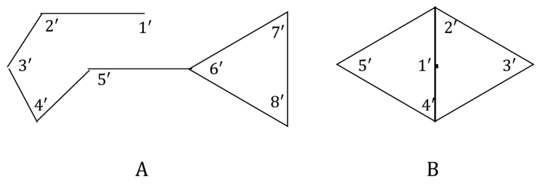
Example 1.
Note that the graph in Figure 1-A has upper approximation neighbourhood system given by
The lower approximation neighbourhood system of is given by and for all .
In Figure 1-B, the graph has upper approximation neighbourhood system given by
The lower approximation neighbourhood system of is given by
Figure 1.
Representation of upper and lower approximation neighbourhood system
Theorem 1.
Let be any simple graph. The family forms a basis of a topology on , where is the intersection set of all upper approximation neighbourhoods containing x in .
Proof.
It is clear that for all . That is, . On the other hand, since for all , then , i.e., . Now we will prove that for every two elements , there is such that . Let and be any two elements in . If , then take to get the desired. Let . Then there is at least one and . Since then for all with . Similarly, since then for all with . In all cases we get that . Take . That is, .
On the other hand, let , that is, . Hence for some . Then and this implies for all . So we have . Hence and , that is, and . Hence .
From the two cases we get . Therefore, forms a basis of a topology on . □
For any simple graph , the topology in the above theorem which is induced by the basis will be called an upper approximated G-topology of a graph and will be denoted by . From the definitions of the basis and an upper approximation neighbourhood system , we get that the family forms a subbasis for an upper approximated G-topological space .
The simple graph of Figure 1-A in Example 1 has an upper approximated G-topological space with a basis , where
In Figure 1-B, the graph has the upper approximated G-topological space with a basis , where
Example 2.
Let be any simple graph. If is an isolated vertex, then it is clear that the set is an open set in the upper approximated G-topological space and also if is an isolated edge, then the set is an open set. Furthermore, if we have an isolated path P in of length two of the form , then the set is an open set. If we have an isolated path P in of length 3 of the form , that is, , then it is easy to see that the upper approximated G-topological space has a basis which is given by .
Theorem 2.
Let P be a path of the form
where . Then the basis of is given by
for all .
Proof.
Note that
and similarly, . For all , we have
Hence,
for all . □
Theorem 3.
The upper approximated G-topological space of a complete graph is an indiscrete space for all .
Proof.
In case , , then it is clear that . That is, is an indiscrete space. If , and is any vertex, then , that is, . Hence, for all , that is, for all . Hence, is an indiscrete space for all . □
Theorem 4.
The upper approximated G-topological space of a complete bipartite graph is an indiscrete space for all .
Proof.
In case , , then it is clear that and . That is, and . Hence, is an indiscrete space. Let and . Let be any vertex. Since , then or . Let . By definition of the complete bipartite graph , . Now we will show that . Let be any vertex. Then . So we have , that is, . Hence, . Then we have and hence . Similarly, if , we get that . Since x was an arbitrary vertex, then is an indiscrete space for all . □
For a cycle graph with , say , we note that for all . That is, the upper approximated G-topological space of is an indiscrete space. Similarly, if or , then we get that for all or for all , respectively. That is, the upper approximated G-topological space of is an indiscrete space for . The following theorem shows that the upper approximated G-topological space of is a discrete space for all .
Theorem 5.
The upper approximated G-topological space of a cycle graph is a discrete space for all .
Proof.
Consider the cycle graph ,
where . By definition of and since for all , we have
and
Now for all , since the cycle graph is a closed path then from the proof of Theorem 2 we have
Hence, . This meams is a discrete space for all . □
The following theorem shows that the Alexandroff topological property will be satisfied for the upper approximated G-topological spaces of locally finite simple graphs, i.e., the arbitrary intersection of open sets is an open set.
In our next work, any simple graph will be locally finite.
Theorem 6.
The upper approximated G-topological space of any simple graph is an Alexandroff space.
Proof.
Let be any simple graph. Let Z be any nonempty subset of . Let be the collection of all the upper approximated neighbourhoods of elements of Z. We will prove that is an open set in . Let . Then for all . Hence for all . So, . Since is locally finite, then is finite and so Z is finite. Hence, is an open set. This proves that the upper approximated G-topological space is an Alexandroff space. □
In the class of locally finite simple graphs , by using the Alexandroff topological property of the upper approximated G-topological spaces , we can define an operator from the vertices set into the upper approximated G-topology by is the smallest open set containing x, . It is clear that for an isolated point in any graph G, and if is an isolated edge, then . Furthermore, if we have an isolated path P in of length two of the form , then .
Theorem 7.
For any simple graph , for all .
Proof.
By the definition of the family and Theorem 1, is an open set in the upper approximated G-topological space for all . By Theorem 1, is an open set containing x. Since is the smallest open set containing x, then
On the other hand, since is the intersection of all open sets containing x, then let for some subset Q of . Then for all , and this implies for all . Ome concludes . Hence, So, □
Theorem 8.
Let be a simple graph. For any two vertices , if and only if .
Proof.
Let be any two vertices and . By Theorem 7, . Since , then . Hence .
Conversely, let . By using Theorem 7 again, we can get that . Then . It mens for all . This implies for all . Hence, . □
Theorem 9.
Let be a simple graph. Then for all , and if and only if is discrete.
Proof.
Let x be any vertex in . It is clear that . Suppose that is any vertex. If , then by Theorem 8, and this is in contradiction with the hypothesis. Hence, for all , i.e., is discrete.
The reverse implication is clear since for all . □
Let be any simple graph and . The closure of X, denoted by , is defined as the intersection of all closed sets containing X in the upper approximated G-topological space . Note that if and only if for every open set G containing x, (see, [1]).
Theorem 10.
For any simple graph and for all , for all .
Proof.
Let . Then for each open set G containing , . Since for all , then for all , i.e., for all . Hence, for all . □
From Theorem 10, for any vertex , for all .
Corollary 1.
Let be any simple graph and . Then if and only if .
4. On Isomorphic Properties
In this section we first study the relationship between isomorphic relations for simple graphs and homeomorphic relations of their upper approximated G-topological spaces. Next, we give some results about some isomorphic properties.
Let and be two simple graphs without isolated vertices. The graphs and are called isomorphic, denoted , if there is a bijective mapping such that if and only if for all . A mapping of a topological space into a topological space is continuous if for all . A mapping is called closed if is closed set in for all closed set . Recall [1] that if a mapping is bijective, closed nd continuous, then it is called a homeomorphism.
Theorem 11.
Let and be two simple graphs and be any mapping of the upper approximated G-topological spaces into . Then is a continuous mapping if and only if for all , implies .
Proof.
Let implies for all . Let O be any subset of and . If then for some . Hence . By the hypothesis we get . Then Hence, is continuous.
Conversely, let be continuous and be any two vertices such that . By Corollary(1) we get , and by continuity of , . Thus, by Corollary(1), we get . □
Theorem 12.
Let and be two simple graphs. Then a mapping is closed if is onto and for all , implies .
Proof.
Let O be any closed set in . Since is onto, then there is a mapping such that . Now we prove that is continuous. Let be arbitrary vertices such that . Hence . By the hypothesis we get . By Theorem 11 is continuous. Hence is closed set and so is a closed mapping. □
Theorem 13.
Let and be two simple graphs. If a mapping is closed and one-to-one, then for all , implies .
Proof.
Let be any two vertices such that . Since is one-to-one, then there is a function such that . Since is one-to-one and closed, it is easy to see that is continuous. This implies that , that is, . □
Theorem 14.
A bijective mapping of two simple graphs and is a homeomorphism if and only if for all , if and only if .
The following theorem shows that the isomorphic relation of simple graphs without isolated vertices gives us the homeomorphic relation of their upper approximated G-topological spaces.
Theorem 15.
Let and be two simple graphs without isolated vertices. If and are isomorphic, then there is a homeomorphism between upper approximated G-topological spaces and .
Proof.
Let be a bijective function such that if and only if for all . Let be any two vertices with . Then we have or . Let . Then there is an edge which joins x and y in . By the isomorphism of and , we get that the edge joins and in , that is, . So, in this case, . Now, in the other case, if , then there is some and . Then, similarly to the first case, we get and , that is, . Hence, . Hence for all , if and only if . Then by Theorem 14, is a homeomorphism of upper approximated G-topological spaces into . □
Note that if a homeomorphic relation of upper approximated G-topological spaces, then the isomorphic relation of induced simple graphs need not be satisfied. For example, by Theorem 4, the complete bipartite graph with has an indiscrete upper approximated G-topological space , and by Theorem 3, has an indiscrete upper approximated G-topological space . So and are homeomorphic, while the graphs and are not isomorphic, since if and , then x and y are joined in but not in .
Recall [1] that the compactness is a topological property. So, by Theorem 15, the compactness is an isomorphic property in the theory of simple graphs. It is clear that the upper approximated G-topological space of any simple graph is a compact space if is finite. The upper approximated G-topological spaces induced by infinite graphs need not be compact. For example, in Figure 3, the simple graph with an infinite vertices set has the subbasis given by . The upper approximated G-topology of the graph is an indiscrete spaces and so it is a compact space.
Also we have that from Theorem 3, the upper approximated G-topology of a complete graph is a discrete space, and if is infinite, then is not a compact space.
The following theorem shows a relationship between connectedness property of upper approximated G-topological spaces and connectedness property of simple graphs.
Theorem 16.
Let be any simple graph without isolated vertices. If the upper approximated G-topological space is a connected space, then is a connected graph.
Proof.
Suppose that is a disconnected simple graph. Consider , the family of all components in , where for all . Now for all , . Then is a nonempty proper open subset of , where . Then is also a nonempty proper open subset of . This means that is a disconnected space which contradicts connectedness of . Hence, is a connected graph. □
Connected simple graphs need not induce connected upper approximated G-topological spaces. For example, by Theorem 5, the cycle graph is a connected graph, and has disconnected upper approximated G-topological space , since it is discrete.
By Theorem 3, the complete graph is connected and has connected the upper approximated G-topological space , since it is indiscrete. Also by Theorem 4, the connected graph has connected the upper approximated G-topological space .
Let be any simple graph. Define as the subset of containing all vertices x with , where denotes the number of elements in . A simple graph is called an upper connected graph if the subgraph of , induced by , is connected. If the relative topology is discrete on the set , then the upper approximated G-topological space will be called upper discrete. For any simple graph , if , then we assume is upper connected and is upper discrete. For the cycle graph , if , then and so is upper connected with not upper discrete. If , then and so is an upper connected graph with which is an upper discrete space. From Theorem 5, for all , and hence is an upper connected graph, and is an upper discrete space. For the complete graph , , and hence is upper connected and is not upper discrete. If , then by Theorem 3, and hence is an upper connected graph having the space which is an upper discrete space.
For the complete bipartite graph , if , then and hence is upper connected with that is not upper discrete. If , then by Theorem 4, and hence is an upper connected graph with upper discrete space ,
Note that in Figure 2-A of Example 2, . So we get that is an upper connected graph for which the space is upper discrete.
In Figure 2-B of Example 2, . So we get that is an upper connected graph, and the space is not upper discrete.
Sari and Kopuzlu, [11] introduced the graphic topological spaces in the theory of undirected graphs induced by a subbasis which is the family of open neighbourhoods of vertices in and proved that the graphic topological space of any locally finite graph is an Alexandroff space. By this property for , we can define the minimal operator in as a function from into which is given by: for all , is the smallest open set in containing x. Since for all and by the two definitions of graphic topological space and an upper approximated G-topological space , we get for all .
Recall [1] that in a topological space , a subset G is called dense in M if , that is, if for all open sets O.
Theorem 17.
Let be an upper connected graph. Then is dense in , where is the set of all vertices in with degrees greater than one.
Proof.
Let . Since is the smallest open set containing x, then to show that for all open sets O in , we will prove that for all . Let . Since x is not isolated, then there is such that . Hence . Hence, . So, there exists some such that . Then , that is, for all . Therefore, is dense in . □
Theorem 18.
Let be an upper connected graph, be the family of smallest open sets of all vertices in and be the family of all minimal sets in . If is a minimal dense set in then there is an onto mapping such that for all .
Proof.
By the form of , the intersection of every pair of distinct elements of is empty set. Since in , there is some for all . Since and , then and it is clear that , that is, . If , then similarly we get that . Hence . Then and we have a contradiction. So, .
Define the mapping of into sending into the single element of . Now we will prove that is onto. Let . We prove that such that . If , then there is such that is a proper subset of . Then . In this case we get that , a contradiction. Hence, such that . □
Theorem 19.
Let be an upper connected graph, be the family of smallest open sets of all vertices in and be the family of all minimal sets in . If is a mapping such that for all , then is a minimal dense set in .
Proof.
It is easy to see that for all there is such that and . Hence we get , that is, is dense in .
To prove that is minimal dense set in , let and . Suppose that such that . Then there is such that and . Since and , that is, , then and so . This is a contradiction. □
5. Some Applications On Radar Charts
The radar chart or web chart is a graphical method in statistics which consists of a sequence of equiangular radii such that each radii represents one of variables (categories) as in Figure 4. The data length of a radii is proportional to the size of data variable relative to the maximum size of the variable across all data points (groups) [21]. In this section we will prove that if the number of categories for a radar chart is large enough, then the upper approximated G-topological space for the corresponding graph of this radar chart is disconnected and discrete. Furthermore, we will show the upper connectedness and upper discreteness for corresponding graphs of radar charts.
In a radar chart, m denotes the number of categories and n denotes the number of groups. The graph denotes the corresponding graph of a radar chart with m categories and n groups. If and , then the corresponding graph of the radar chart will be a cycle graph . So, by Theorem 5, the upper approximated G-topological space is discrete and so disconnected if . Since , then then space is also upper discrete.
In Figure 6-A, the radar chart has categories and groups. The graph has vertices set , and the upper approximated G-topological space has a subbasis . So we get that is indiscrete and so connected. Since , then is upper discrete.
In Figure 5-A, the radar chart has categories and groups. The corresponding graph in Figure 6-B has vertices set , and the upper approximated G-topological space has a subbasis given by
and So we get that is discrete and so disconnected. Since , then is upper discrete, and is upper connected.
Figure 5.
Radar chart with , and ,
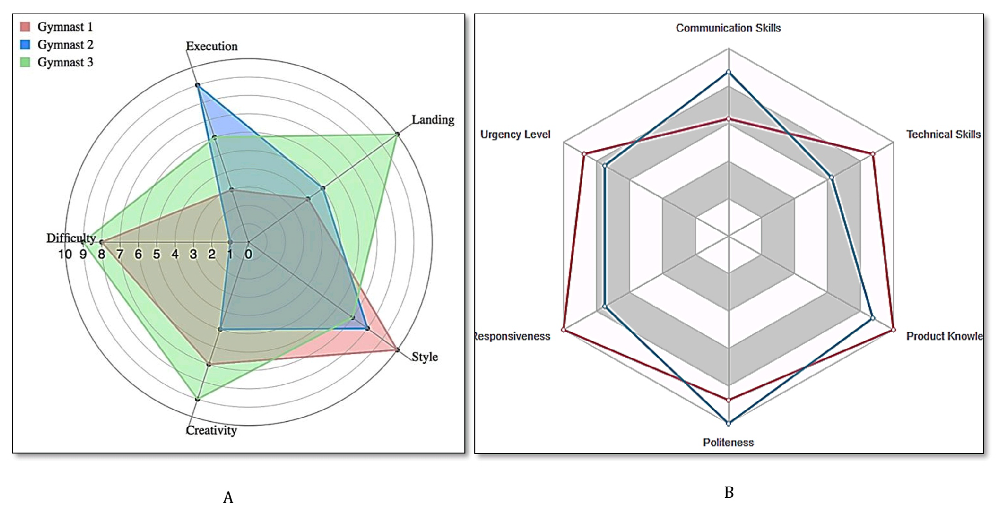
Figure 6.
Representation of radar chart with (, ), (, ) and (, )
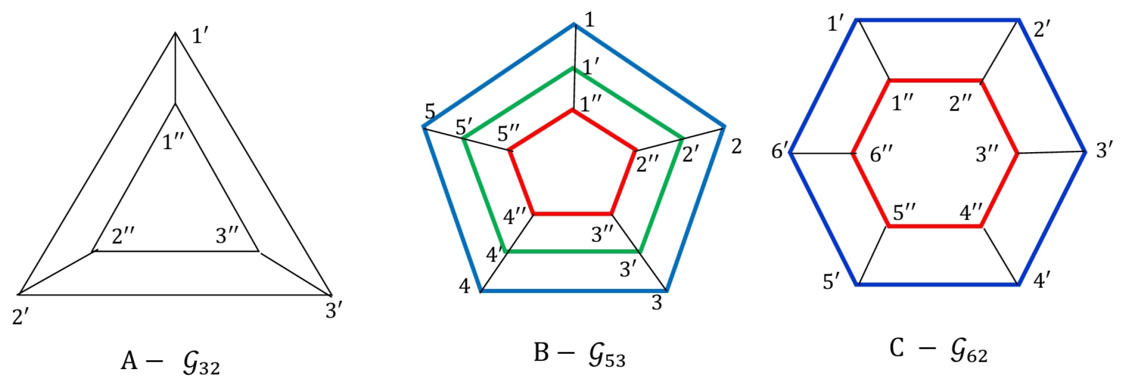
In Figure 5-B, the radar chart has categories and groups. The corresponding graph in Figure 6-C has vertices set , and the upper approximated G-topological space has a subbasis similar for then graph above. We get that for all . Therefore, we get that is discrete and so disconnected. Since , then is upper discrete, and is upper connected.
The discrete and upper discrete properties are also satisfied if there is intersection between group charts such as in the radar chart in Figure 7-A (see [22]). The radar chart has categories and groups with intersection points between groups. The corresponding graph in Figure 7-B has vertices set
with intersection vertices 2, 3 and 5. The upper approximated G-topological space has a subbasis given in Table 1. So, by the details in Table 1, we get that is discrete and so disconnected. Since , then is upper discrete.
Now, in general we study the connectedness and discreteness for the corresponding graphs of the radar charts with categories and groups. The corresponding graph in Figure 8 has vertices set . For the upper approximated G-topological space , some upper approximation neighbourhoods are given in Table 2. Similarly, for all vertices x that lie on the groups 1,2, and n, we have .
For all and , we have
Hence
So, we conclude that the upper approximated G-topological space is discrete and so disconnected. Since , then is upper discrete.
6. Conclusions
We have defined a new topology, called the upper approximated G-topology, on the vertices set of a simple graph and investigated several topological properties (discreteness, compactness, connectedness) related to this topology. The topology is define by using upper approximation neighbourhood systems of graphs. In particular, the study includes some well known graphs, as complete graphs , cycle graphs and complete bipartite graphs . Some applications to radar charts are given. We expect that our study can be applied to other classes of graphs and other topological properties.
Author Contributions
Conceptualization, H.A., L.D.R.K. and H.A.O.; investigation, H.A., L.D.R.K. and H.A.O.; resources, H.A.O. All authors have read and agreed to the published version of the manuscript.
Funding
This research work was funded by Umm Al-Qura University, Saudi Arabia under grant number: 25UQU4350370GSSR01
Data Availability Statement
The original contributions presented in the study are included in the article, and further inquiries can be directed to the corresponding author.
Acknowledgments
The authors extend their appreciation to Umm Al-Qura University, Saudi Arabia for funding this research work through grant number: 25UQU4350370GSSR01.
Conflicts of Interest
The author declares no conflicts of interest.
References
- Dugundji, J. Topology; Allyn and Bacon, Inc.: Boston, 1966. [Google Scholar]
- Bondy, J.A.; Murty, U. Graph theory. In Graduate Texts in Mathematics; Springer: Berlin, 2008. [Google Scholar]
- Kiliciman, A.; Abdu, K.A. Topological spaces associated with simple graphs. J. Math. Anal. 2018, 9, 44–52. [Google Scholar]
- Abdu, K.A.; Kiliciman, A. Topologies on the edges set of directed graphs. J. Math. Comp. Sci. 2018, 18, 232–241. [Google Scholar] [CrossRef]
- Amiri, S.M.; Jafarzadeh, A.; Khatibzadeh, H. An Alexandroff topology on graphs. Bull. Iran. Math. Soci. 2013, 39, 647–662. [Google Scholar]
- Nada, S.; Atik, A.E.F.; Atef, M. New types of topological structures via graphs. Math. Method Appl. Sci. 2018, 41, 5801–5810. [Google Scholar] [CrossRef]
- Nianga, C.G.; Canoy, S. On topologies induced by graphs under some unary and binary operations. Eur. J. Pure. Appl. Math. 2019, 12, 499–505. [Google Scholar] [CrossRef]
- Nianga, C.G.; Canoy, S. On a finite topological space induced by Hop neighbourhoods of a graph. Adv. Appl. Dis. Math. 2019, 21, 79–89. [Google Scholar]
- Anabel, E.G.; Sergio, R.C. On a topological space generated by Monophonic eccentric neighbourhoods of a graph. Eur. J. Pure and App. Math. 2021, 14, 695–705. [Google Scholar]
- Gamorez, A.; Nianga, C.G.; Canoy, S. Topologies induced by neighbourhoods of a graph under some binary operations. Eur. J. Pure Appl. Math. 2019, 12, 749–755. [Google Scholar] [CrossRef]
- Sari, H.K.; Kopuzlu, A. On topological spaces generated by simple undirected graphs. AIMS Math. 2020, 5, 5541–5550. [Google Scholar] [CrossRef]
- Zomam, H.O.; Othman, H.A.; Dammak, M. Alexandroff spaces and graphic topology. Adv. Math. Sci. J. 2021, 10, 2653–2662. [Google Scholar] [CrossRef]
- Othman, H.A.; Al-Shamiri, M.; Saif, A.; Acharjee, S.; Lamoudan, T.; Ismail, R. Pathless topology in connection to the circulation of blood in the heart of human body. AIMS Math. 2022, 7, 18158–18172. [Google Scholar] [CrossRef]
- Shokry, M.; Aly, R.E. Topological properties on graph vs medical application in human heart. Int. J. Appl. Math. 2013, 15, 1103–1109. [Google Scholar]
- Othman, H.A.; Ayache, A.; Saif, A. On directed graphs with L2—directed topological spaces. Filomat 2023, 37, 10005–10013. [Google Scholar] [CrossRef]
- Abu-Gdairi, R.; El-Atik, A.A.; El-Bably, M.K. Topological visualization and graph analysis of rough sets via neighborhoods: A medical application using human heart data. AIMS Mathematics 2023, 8, 26945–26967. [Google Scholar] [CrossRef]
- Yao, Y. On generalized rough set theory, rough sets, fuzzy sets, data mining and granular computing. Inter. Proc. 9th Int. Conf. 1999, 44–51. [Google Scholar]
- Chiaselotti, G.; Ciucci, D.; Gentile, T.; Infusino, F. Rough set theory and digraphs. Fund. Inform. 2017, 153, 291–325. [Google Scholar] [CrossRef]
- Atik, A.; Nawar, A.; Atef, M. Rough approximation models via graphs based on neighborhood systems. Granular Computing 2021, 6, 1025–1035. [Google Scholar] [CrossRef]
- Guler, A. Different neighbourhoods via ideals on graphs. J. Math. 2022, 2022, 9925564. [Google Scholar] [CrossRef]
- Michael, P.; Pooya, M. Multidimensional mechanics: Performance mapping of natural biological systems using permutated radar charts. PLOS ONE 2018. [Google Scholar] [CrossRef]
- Joan Saary, M. Radar plots: A useful way for presenting multivariate health care data. J. Clinical Epidem. 2008, 60, 311–317. [Google Scholar]
Figure 2.
Representation of upper approximated G-topology
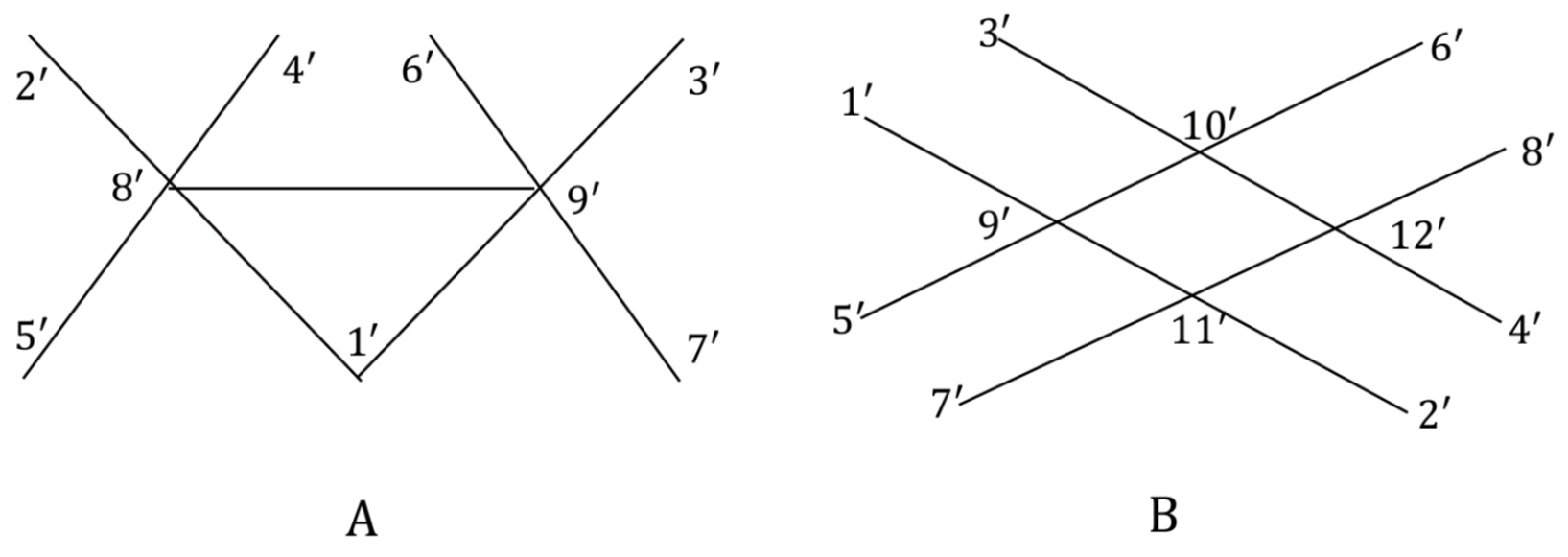
Figure 3.
Graphical representation with infinite vertices set
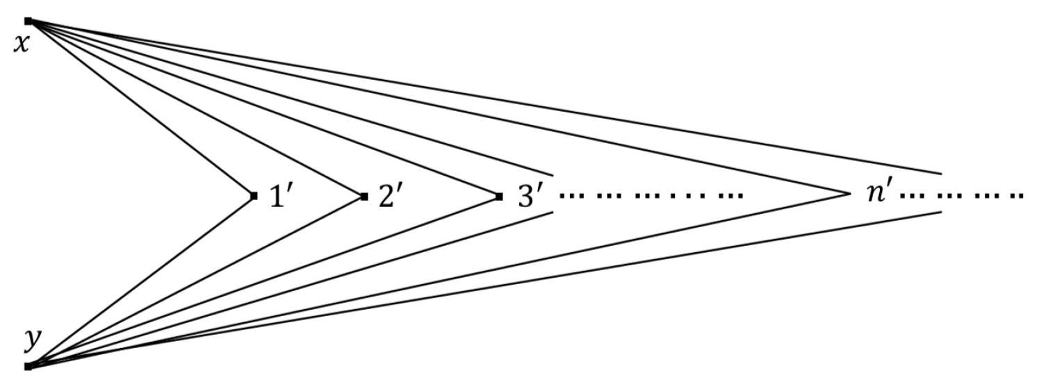
Figure 4.
General radar chart
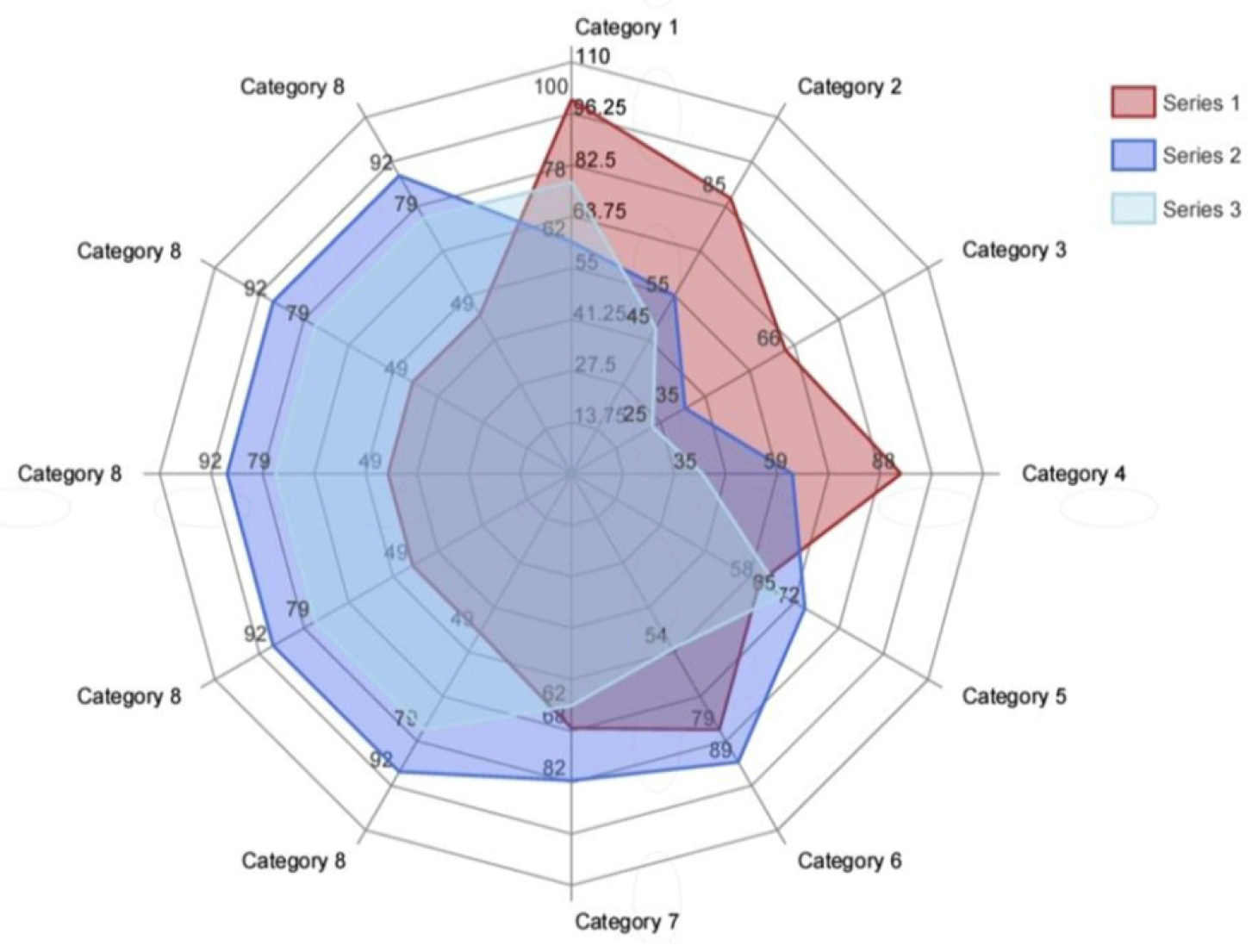
Figure 7.
Radar chart and its representation with ,
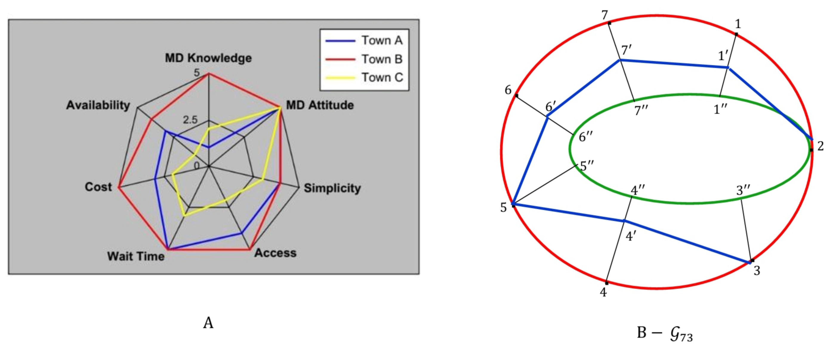
Figure 8.
Representation of general radar chart
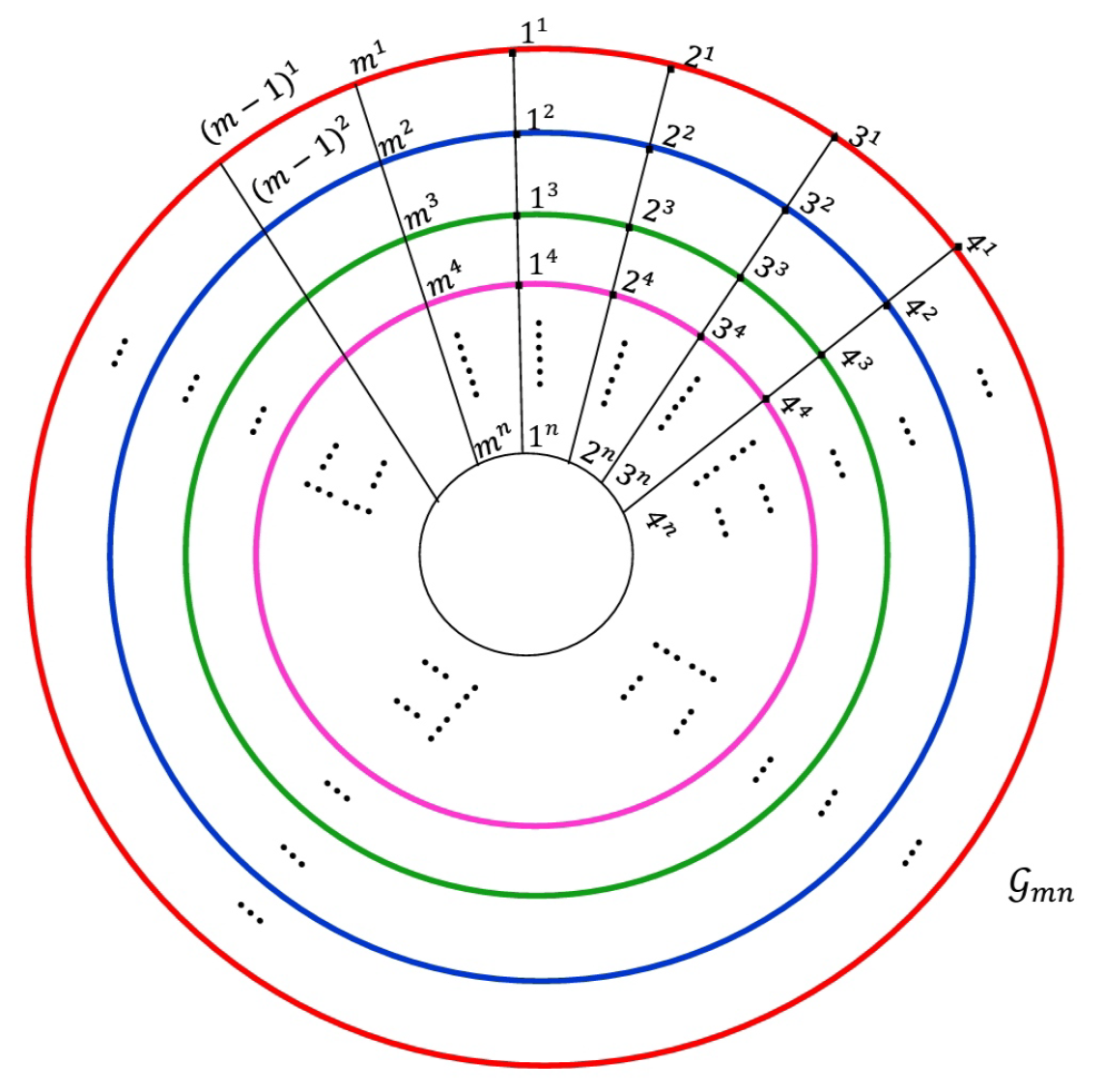

Table 1.
An upper approximation neighbourhood system of graph
| x | |||
|---|---|---|---|
| 1 | 1 | ||
| 2 | 1 | ||
| 3 | 1 | ||
| 4 | 1 | ||
| 5 | 1 | ||
| 6 | 1 | ||
| 7 | 1 | ||
| 1 | |||
| 1 | |||
| 1 | |||
| 1 | |||
| 1 | |||
| 1 | |||
| 1 | |||
| 1 | |||
| 1 | |||
| 1 |
Table 2.
Some of upper approximation neighbourhoods of graph
| x | |||
|---|---|---|---|
| 1 | |||
| 1 | |||
| 1 | |||
| 1 | |||
| 1 | |||
| 1 | |||
| 1 | |||
| 1 | |||
Disclaimer/Publisher’s Note: The statements, opinions and data contained in all publications are solely those of the individual author(s) and contributor(s) and not of MDPI and/or the editor(s). MDPI and/or the editor(s) disclaim responsibility for any injury to people or property resulting from any ideas, methods, instructions or products referred to in the content. |
© 2025 by the authors. Licensee MDPI, Basel, Switzerland. This article is an open access article distributed under the terms and conditions of the Creative Commons Attribution (CC BY) license (http://creativecommons.org/licenses/by/4.0/).
Copyright: This open access article is published under a Creative Commons CC BY 4.0 license, which permit the free download, distribution, and reuse, provided that the author and preprint are cited in any reuse.


