

Submitted:
27 January 2025
Posted:
28 January 2025
You are already at the latest version
Abstract
This paper suggests a generalization of covariates shifts to study distributional impacts on inequality and distributional measures. It builds on the recentered influence function (RIF) regression method designed for location shifts on covariates, but it extends to general policy interventions such as location-scale or asymmetric interventions. Numerical simulations for Gini, Theil and Atkinson indexes show it has a very good performance on a myriad of cases and distributional measures. An empirical application to studying changes in Mincerian equations illustrates the method.
Keywords:
Influence functions
; RIF regression
; Gini
; Atkinson
; counterfactual distributions
1. Introduction
The recentered influence function (RIF) regression has become a powerful tool for analyzing how changes in covariates impact the distributional statistics of an outcome variable. It is particularly valuable in the study of income distribution, inequality, and poverty. Introduced in the seminal paper by [1], this method consists of a regression on a suitable transformation of the outcome. The transformation is based on the influence function of the feature of the distribution of the outcome that is of interest. The influence function—a fundamental statistical concept that captures how individual observations affect unconditional statistics- is readily available from textbooks,1 making the approach very convenient and easy to implement. In a nutshell, by regressing the RIF on covariates, researchers can estimate the marginal effects of these covariates on various distributional measures, offering a flexible and insightful approach to understanding economic and social disparities.
RIF regression has been widely adopted in empirical research, particularly for studying unconditional quantiles. In this case, the parameter of interest is usualy referred to as the unconditional quantile effect (UQE), and the RIF regression is called unconditional quantile regression (UQR). Other distributional measures such as the Gini coefficient, the Theil index, and polarization indices can be readily implement as long as the influence function is known. The method has gained traction across disciplines, including labor economics, health economics, and public policy, where understanding the distributional effects of observed characteristics is essential. Subsequent research has further developed RIF-based methodologies. For instance, [3] provide an extensive derivation of influence functions for various distributional statistics, which serve as foundational elements in RIF models. Additionally, [4] extend RIF regression to Oaxaca-Blinder decomposition models, while further refinements have been made by [5] and [6].
The original RIF regression is in fact just one potential use of these effects. That is, the model of [1] is concerned with a location-shift effect in one covariate on the unconditional distribution of the variable of interest. In other words, it shifts only the location of distribution of that particular covariate (or a marginal shift in the probability for a binary regressor). However, in practice, a policy intervention not only refers to a uniform increase in the entire range of the covariate but could also represent a general change. A broader approach may consider changes in both location and scale, or asymmetric changes of the covariate. This paper proposes a simple and intuitive representation for these types of effects, using a parametric model. Our contribution is to study general parametric covariate shifts for the general RIF environment, thus proposing a simple application to any distributional functional. As a result we can evaluate any policy intervention that has any general functional form.
Different approaches have been recently developed for extending the location-only effects, mostly concerned with UQR. [7] consider this case as a way to transform the status quo population, although they do not consider the limiting/marginal case as in [1].2 They, however, do not develop the specific methodologies for general shifts in covariates and for different functionals. [9] consider location and scale shift effects to estimate UQR models and it provides a framework for general policy interventions. The estimation procedure, however, is not based on RIF regressions, but on maximum likelihood.3 Other work extending the UQR methods include, for instance, [10] for a two sample problem, [11] for the high dimensional case, and [12] consider the relationship between conditional quantiles and unconditional quantiles.
Our Monte Carlo simulations use as a distributional functional the Gini coefficient to illustrate how this method works. The simulations show that the proposed method works very well for many parametric functions of a shift. Finally, we propose an empirical application to study the effect on inequality of different policy interventions with different shifts. In particular, we study changes in education and experience in a Mincerian equation framework.
This paper is organized as follows. Section 2 reviews the RIF regression method and presents our proposed estimands for different shift covariate effects. This section also discusses some empirical examples where the proposed estimators can be used in the literature. Section 3 presents the corresponding estimators and discusses their asymptotic properties. Section 4 shows finite sample evidence on the estimator performance using Monte Carlo experiments. Section 5 applies the proposed estimators to the case of shifts in education and age in a Mincer equation. Finally, Section 6 concludes.
2. RIF Regression
2.1. RIF Regression Framework for Pure Location-Shifts
Consider a functional defined on the distribution function of a random variable Y. Changes in v that measure the influence or impact of a given observation through are studied using the influence function (IF). More formally, the IF is the directional derivative of at and measures the effect of a small perturbation in . The IF can be calculated at each data point in the domain of Y. Let y be be such point, that contains a Dirac probability mass of , such that we define
When is evaluated at Y, it becomes a random variable. Importantly, it has zero mean by construction, that is, . For example, if , the -quantile of , then
Note that
because The appendix contains the influence function for the Gini, Atkinson, and Theil indices.
The recentered influence function (RIF) is simply defined as
and by the previous result it satisfies This is a key property as it allows to implement the Law of Iterated Expectations and to work with conditional models. In particular, if we consider a set of covariates of interest X, then we have that
[1] key result is based on modeling of the conditioning part, using standard regression tools, as this is referred to as RIF regression. Then, by the properties above, integrating over X links to the unconditional statistic of interest, i.e. .
[1] focuses on marginal effects on covariates X, modeled as a location shift where is a small real valued perturbation. Changes in X have a corresponding effect on Y, the outcome of interest. To study this, consider a statistical tool built upon the IF. Define as the distribution of Y after the perturbation in X. Then we consider a functional derivative given by
The last equality is valid if we assume that limit and expectation are interchangeable, which we assume throughout the paper. In fact, if we assume that is differentiable at any point x, then we obtain the main result of RIF regression models, that is,
measures the impact of a given location shift in covariates on the unconditional functional statistic v of Y. Statistically, the expression for , is called an average derivative, and is an object whose estimation has been thoroughly studied. An excellent textbook reference is chapter 4 of [13].
2.2. General Unconditional Effects
While [1] focus mainly on a location shift, one can consider a general shift on a given covariate,
where , , and as a function of the function is a continuously differentiable function. Then we consider general unconditional effects as
for general h functions.
Here we index the unconditional effect by h, which denotes the type of counterfactual policy analyzed. Naturally, depending on the particular form of we obtain different effects. Here are few examples:
- Location shift This is the case developed above taken from [1] analysis that consider a location shift change in one covariate of the form
- Location-scale shiftwhere , and are continuously differentiable functions with and , respectively. Here acts as a shrinking parameter such that an increment in this parameter reduces the overall impact of the X variable. The pure location shift in [1] can be obtained by setting and . [9] have a similar shift written in a different manner. In fact different alternatives can be developed based on how to combine the location and scale joint shifts.
- Asymmetric shiftwhere , and the map satisfies: , , and is continuously differentiable. The factor is maximum value in the support of X or an upper bound. The parameter determines the asymmetry of the shift effecs: if then the shift is biased towards upper values, if the shift is biased towards lower values, if this would be a pure location-shift. Although this type of shift was applied as a numerical simulation exercise in [14], the novelty of our proposal is to include it analytically within the RIF regression strategy.
From the definition of RIF, one can compute the parameter of interest in equation for the three cases described previously. Let for a given functional . Using the same derivation strategy as in Section 2.1 above, it is straightforward to compute that the estimand of interest is
The estimand is the product of the derivative of two functions. First the function, which depends on the functional of interest, and second, of which depends on the type of counterfactual policy. The formula in (7) can then be applied to each particular effect that the user is trying to analyze.
-
Location shiftThis is indeed the estimand of [1] and the most popular amongst RIF regression empirical applications.
-
Location-scale shift
- Asymmetric shift
2.3. Empirical Examples to Motivate the Estimands
Here we discuss some empirical examples where these models could be used.
Effect of increasing education on wage inequality. In a Mincer equation, log wages are modeled as a function of certain observable covariates such as years of education. Changes in education levels have different effects on income inequality and a positive shift may result in augmenting it, the so-called `paradox of progress’ (see [15]). A study of the effect of a shift in education on wage inequality could be implemented using our proposed framework. We can accommodate a counterfactual policy experiment where there may be not only a general increase in the education level but also a change in its dispersion or an asymmetric shift towards the highest possible level of education.
Smoking and birth weight. Consider a cigarrete consumption tax. Under some assumptions, the consumption X will be reduced to for some that depends on the elasticities of the supply and demand. One might wonder about the final impact of this tax policy on the distribution of birth weights. This is analyzed in [9].
Wage controls and earnings distribution [16] studies the effect of a more uniform (less dispersion) distribution of wage control brackets on the distributions of earnings, in the context of a policy that was implemented during War World II.
3. Generalized RIF Estimator
The proposed estimands can be estimated using the RIF regression method. This is implememented in three steps.
First, we need to specify a model for the function, that is, the relationship between the RIF of the v functional together with an ad-hoc model on how it relates to the covariates, i.e., . Let be such estimator. Assume a parametric model
for some parameter with true value at . The estimator is then , where is a consistent estimator of . [1] have several alternatives, for which RIF OLS and RIF Logit are the most commonly used. Similar procedures can be applied to any functional as it is usually done in the applied literature. In turn, this requires that the proposed model is an appropriate representation of the true model. can then be interpreted as the parameters from the RIF regression model and as the corresponding estimator.
For example, a third degree polynomial is a popular choice:
Second, depending on the proposed model different alternatives arise as show in Section 2.2. This depends on the policy intervention of interest and the associated shift in covariates. Then, we can compute for each case. This derivative may also include estimated parameters. Let be such estimator. Assume a parametric model
for some parameter with true value at and that is a consistent estimator of . Thus, the estimator is .
Third, the unconditional effects can then be obtained by sample averages of the product formed by the two elements in the last paragraphs.
Now define for . Consistency of will follow from a uniform law of large numbers over , and the correct specification of the parametric model for . For a uniform law of large numbers, sufficient conditions can be found in Lemma 4.3 in Newey and McFadden [17].
Assumption A1.
Assume that is continuous at with probability one, and there is a neighborhood of such that .
The correct specification of the model for is quite challenging. Indeed, it is unlikely that a parametric specification is the correct one. However, one can view an specification like the one in (9) as a series approximation to the true model. A rigourous treatment is provided in [1] for the case .
Deriving the asymptotic normality of our estimators is more complex and requires a more intricate analysis. If the influence function were observed, it would exhibit the standard parametric asymptotic convergence rate, i.e., , as this follows from a standard OLS (or Logit) analysis. However, in most cases, the IF must be estimated and often involves nonparametric components, such as densities. This necessitates a case-by-case asymptotic analysis for different estimators. As noted by Firpo et al. [1], p.962, “because the density is nonparametrically estimated by kernel methods, the rate of convergence of the three estimators will be dominated by this slower term.” [5] derive the asymptotic distribution for the functionals used here (Gini, Theil, Atkinson), and the asymptotic distribution of our proposed estimators can, in principle, be obtained via the delta method. For the UQR case, the Supplemental Appendix in [1] provides a detailed example for the location-shift effect, which can be extended to any shift function of X. A specific extension is developed by [9], albeit without relying on RIF methods.
Thus, while the asymptotic normality of our proposed estimators can be derived, it involves additional technical challenges, and we leave this as an avenue for further research. In our implementation, we conduct inference using the wild bootstrap, a common approach in RIF regression methods.
4. Monte Carlo Experiments
Consider the Gini coefficient as our distributional target of interest v and the following data generating process (DGP):
with where and is a random variable that is independent of . The chosen value parameters will exclude . See the Appendix for the details on the Gini index computation together with the RIF.
Then for each DGP we compute by a simulation with sample size. In all cases, we replace in eq. (11) thus obtaining and computing numerically for .
We consider the following cases:
- Pure location shift: and .
- Pure scale shift: and .
- Location-Scale shift: and .
- Asymmetric shift: and . Here we set such that no values in the simulations will exceed this.
For the RIF regression we use a third degree polynomial such that
thus,
for .
Then, for the location and scale shifts we have
and
with ; and the parameters are estimated by OLS as in the RIF regression method.
Then, for the asymmetric shift we use
For the simulations we consider the cases of (Table 1) and (Table 2), using . All DGPs and simulation exercises show that the proposed implementation works. Bias and variance reduce monotonically as the sample size increase. Note that, as expected, the case of asymmetric shift with coincides with the location-shift effect. Moreover, the method works for all shifts models.
5. Empirical Application
This section presents an empirical application. We use an extract from the Merged Outgoing Rotation Group of the Current Population Survey of 1983, 1984 and 1985 for males only. More details about the data can be found in [18]. The variable of interest is Y, the hourly wage, and the covariates X are an indicator of whether the individual is unionized, years of education, whether he is married, non-white and his experience. We use a cubic specification in all continuous covariates to give some flexibility to the RIF model.
The studied effects correspond to education (Table 3) and experience (Table 4) in order to simulate different interventions and their potential effects on measures of inequality. We consider the estimators of the location, scale and asymmetric effects discussed above for the Gini, Theil and Atkinson indexes (see the Appendix for more details on each index). All indexes are multiplied by 100 and all effects correspond to a change in education/experience on the corresponding shift. Figure 1 and Figure 2 shows the modeled shift for each year of education/experience depending on the value chosen for .
Consider first the effect of education in Table 3. The location effect is positive while the scale effect is negative for all cases. This determines that while a positive shift in education levels has resulted in augmenting inequality (this is also called the `paradox of progress’ by different authors), a reduction in the overall impact of education has a decreasing effect on inequality. In fact, the location-scale joint effect is negative, thus reducing inequality. In the case of the asymmetric shift, note that hourly wages distribution is more equalitarian when the shift is biased towards lower educational levels (), as long as inequality is measured using the Gini or Theil coefficient. However, if the index used is more inequality-averse (Atkinson(1) and Atkinson(2)), then all effects are unequalizing.
Consider now the effect of experience in Table 4. In this case, the effects are clearly negative for both location and scale effects. In fact, in all cases there is a reducing effect on inequality measured by all indices. In the case of asymmetric change, the equalizing effect is greater when the increase in experience is biased towards lower levels ().
6. Concluding Remarks
This paper proposes a simple generalization of covariates shifts to study distributional impacts on inequality and distributional measures. It builds on RIF regression methods designed for location shifts on covariates as in [1], and it extends its use using a similar framework of [9]. The simulations show it has a very good performance on a myriad of cases.
This line of research can be extended in several directions. First, more accurate asymptotic expansions can be obtained if the asymptotic distribution of functionals estimators of the influence functions are known. Moreover, different approximation and numerical methods can be used to estimate them when there is no analytical solution. Second, calibrated covariates shifts can be considered to match empirical policy interventions. For instance, any targeted policy intervention can be mapped into a counterfactual distribution of covariates, from which we can apply our proposed method.
Funding
This research received no external funding.
Data Availability Statement
Dataset available on request from the authors.
Conflicts of Interest
The authors declare no conflicts of interest.
Appendix A. Functionals and Their RIF
Appendix A.1. Gini Index
The Gini coefficient is defined as
where and . Note that if we define then , that is, the term acquires the classical interpretation of the area under the Lorenz Curve given by the expression .
Following [6], and after some algebra, the RIF for the Gini index can be written as:
Appendix Sample Estimator
Assume a random sample , we use a plug-in estimator of the previous equation. First, following [19], consider the observations ordered from smallest to largest , then
Finally, the rest of the components are estimated as follows
Appendix Theil Index
The Theil index is defined as
where and .
Using this notation, the RIF of the Theil is:
Appendix Sample Estimator
Assume a random sample , the statistics to implement the RIF as a plug-in estimator are:
Appendix Atkinson Index
The Atkinson index is defined as
where , , and is an inequality aversion parameter. The parameter defines the type of social preferences and is a value set by the researcher. The two extreme cases are , when the inequality index reflects a utilitarian welfare function () while if it is a Rawlsian function (W is a Leontief type function).
The RIF for the Atkinson index is:
where
and
Appendix Sample Estimator
Assume a random sample , the statistics to implement the RIF as a plug-in estimator are:
where .
References
- Firpo, S.; Fortin, N.; Lemieux, T. Unconditional quantile regression. Econometrica 2009, 77(3), 953–973. [Google Scholar]
- van der Vaart, A. Asymptotic Statistics; Cambridge University Press: Cambridge, 1998. [Google Scholar]
- Essama-Nssah, B.; Lambert, P. Chapter 6. Influence Functions for Policy Impact Analysis. In Inequality, Mobility and Segregation: Essays in Honor of Jacques Silber Research on Economic Inequality; 2015; Vol. 20, pp. 135–159. [Google Scholar]
- Fortin, N.; Lemieux, T.; Firpo, S. Ashenfelter, O., Card, D., Eds.; Decomposition methods in economics. In Handbook of Labor Economics; Elsevier: Amsterdam, 2011. [Google Scholar]
- Firpo, S.; Pinto, C. Identification and Estimation of Distributional Impacts of Interventions Using Changes in Inequality Measures. Journal of Applied Econometrics 2016, 31(3), 457–486. [Google Scholar] [CrossRef]
- Firpo, S.; Fortin, N.; Lemieux, T. Decomposing Wage Distributions Using Recentered Influence Function Regressions. Econometrics 2018, 6(3), 41. [Google Scholar] [CrossRef]
- Chernozhukov, V.; Fernández-Val, I.; Melly, B. Inference on counterfactual distributions. Econometrica 2013, 81(6), 2205–2268. [Google Scholar] [CrossRef]
- Martinez-Iriarte, J. Sensitivity Analysis in Unconditional Quantile Effects. Working Paper.
- Martínez-Iriarte, J.; Montes-Rojas, G.; Sun, Y. Unconditional Effects of General Policy Interventions. Journal of Econometrics 2024, 238(2), 105570. [Google Scholar] [CrossRef]
- Inoue, A.; Li, T.; Xu, Q. Two Sample Unconditional Quantile Effect. ARXIV. Available online: https://arxiv.org/pdf/2105.09445.pdf.
- Sasaki, Y.; Ura, T.; Zhang, Y. Unconditional quantile regression with high-dimensional data. Quantitative Economics 2022, 13, 955–978. [Google Scholar] [CrossRef]
- Alejo, J.; Galvao, A.F.; Martinez-Iriarte, J.; Montes-Rojas, G. Unconditional Quantile Partial Effects via Conditional Quantile Regression. Journal of Econometrics 2024, 105678. [Google Scholar] [CrossRef]
- Pagan, A.; Ullah, A. Nonparametric Econometrics 1999.
- Battiston, D.; Garcia-Domench, C.; Gasparini, L. Could an Increase in Education raise Income Inequality? Evidence for Latin America. Latin American Journal of Economics 2014, 51, 1–39. [Google Scholar] [CrossRef]
- Bourguignon, F.; Lustig, N.; Ferreira, F. The Microeconomics of Income Distribution Dynamics; Oxford University Press: Washington, 2024. [Google Scholar]
- Vickers, C.; Ziebarth, N.L. The Effects of the National War Labor Board on Labor Income Inequality. Working Paper.
- Newey, W.K.; McFadden, D. Engle, R.F., McFadden, D.L., Eds.; Large Sample Estimation and Hypothesis Testing. In Handbook of Econometrics; chapter 36; Elsevier, 1994; Vol. 4, pp. 2111–2245. [Google Scholar] [CrossRef]
- Lemieux, T. Increasing residual wage inequality: Composition effects, noisy data, or rising demand for skill? American Economic Review 2006, 96(3), 461–498. [Google Scholar] [CrossRef]
- Lambert, P. The distribution and redistribution of income; Manchester University Press: Manchester, 2001. [Google Scholar]
| 1 | For some theory, see [2]. |
| 2 | [8] develops a sensitivity analysis procedure that considers both the marginal and non-marginal (global) effects on unconditional quantiles when covariates are discrete. |
| 3 | Another interesting aspect of UQEs is that there is a variety of methods to estimate them. Indeed, [1] rigorously derive three methods. |
Figure 1.
Asymmetric shift, education.
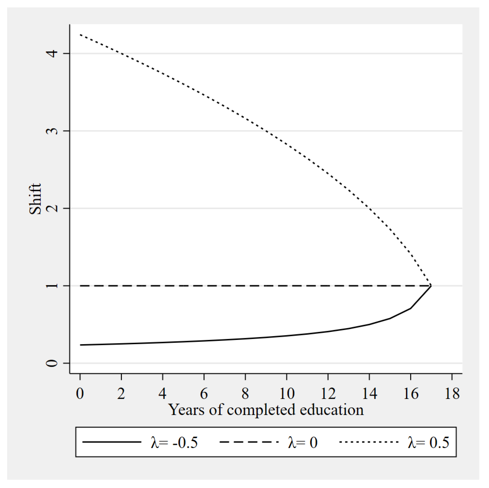
Figure 2.
Asymmetric shift, experience.
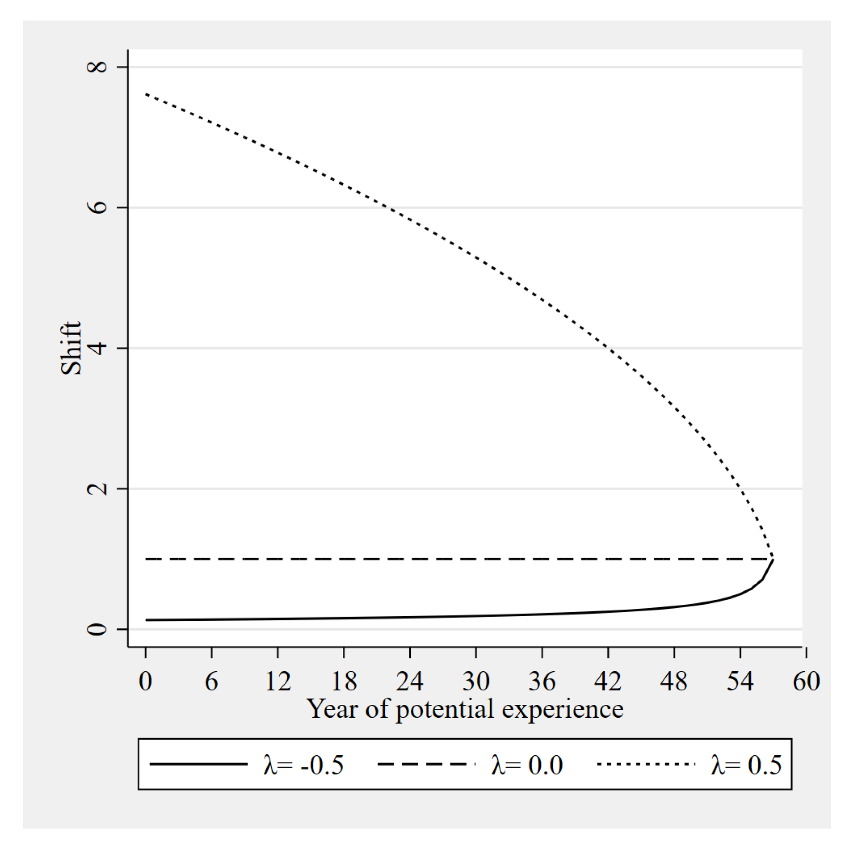

Table 1.
Gini index; .
| Effect | n | ||||||
|---|---|---|---|---|---|---|---|
| Bias | Var | MSE | Bias | Var | MSE | ||
| 50 | -0.0044 | 0.7563 | 0.7564 | -0.1031 | 2.9639 | 2.9745 | |
| 100 | 0.0081 | 0.3482 | 0.3483 | -0.0416 | 1.3842 | 1.3860 | |
| Location | 500 | -0.0086 | 0.0547 | 0.0548 | -0.0260 | 0.2176 | 0.2183 |
| 1000 | -0.0066 | 0.0299 | 0.0299 | -0.0184 | 0.1153 | 0.1157 | |
| 5000 | -0.0005 | 0.0062 | 0.0062 | 0.0020 | 0.0252 | 0.0252 | |
| 50 | -0.1141 | 2.2196 | 2.2326 | 0.0156 | 6.9623 | 6.9625 | |
| 100 | -0.1114 | 1.0436 | 1.0560 | 0.0144 | 3.3553 | 3.3555 | |
| Scale | 500 | -0.0601 | 0.2052 | 0.2088 | -0.0307 | 0.6320 | 0.6329 |
| 1000 | -0.0418 | 0.1078 | 0.1096 | -0.0195 | 0.3407 | 0.3411 | |
| 5000 | -0.0088 | 0.0205 | 0.0206 | -0.0039 | 0.0606 | 0.0606 | |
| 50 | -0.1185 | 3.5751 | 3.5891 | -0.0876 | 10.4689 | 10.4766 | |
| 100 | -0.1033 | 1.7181 | 1.7288 | -0.0273 | 5.2379 | 5.2387 | |
| Both | 500 | -0.0688 | 0.2923 | 0.2970 | -0.0568 | 0.8887 | 0.8920 |
| 1000 | -0.0485 | 0.1612 | 0.1635 | -0.0379 | 0.4704 | 0.4718 | |
| 5000 | -0.0094 | 0.0324 | 0.0325 | -0.0019 | 0.0882 | 0.0883 | |
| 50 | 0.0048 | 0.1453 | 0.1453 | -0.0455 | 0.5998 | 0.6019 | |
| 100 | 0.0112 | 0.0658 | 0.0659 | -0.0179 | 0.2760 | 0.2763 | |
| Asymmetric | 500 | 0.0016 | 0.0107 | 0.0107 | -0.0098 | 0.0439 | 0.0440 |
| () | 1000 | 0.0019 | 0.0057 | 0.0057 | -0.0066 | 0.0235 | 0.0236 |
| 5000 | 0.0033 | 0.0012 | 0.0012 | 0.0018 | 0.0052 | 0.0052 | |
| 50 | -0.0044 | 0.7563 | 0.7564 | -0.1031 | 2.9639 | 2.9745 | |
| 100 | 0.0081 | 0.3482 | 0.3483 | -0.0416 | 1.3842 | 1.3860 | |
| Asymmetric | 500 | -0.0086 | 0.0547 | 0.0548 | -0.0260 | 0.2176 | 0.2183 |
| () | 1000 | -0.0066 | 0.0299 | 0.0299 | -0.0184 | 0.1153 | 0.1157 |
| 5000 | -0.0005 | 0.0062 | 0.0062 | 0.0020 | 0.0252 | 0.0252 | |
| 50 | -0.0365 | 4.3397 | 4.3410 | -0.2329 | 16.0205 | 16.0748 | |
| 100 | -0.0086 | 2.0279 | 2.0280 | -0.0939 | 7.6135 | 7.6223 | |
| Asymmetric | 500 | -0.0350 | 0.3114 | 0.3127 | -0.0665 | 1.1873 | 1.1917 |
| () | 1000 | -0.0270 | 0.1729 | 0.1737 | -0.0473 | 0.6259 | 0.6281 |
| 5000 | -0.0059 | 0.0362 | 0.0363 | 0.0031 | 0.1357 | 0.1357 | |
Note: calculations based on 1000 Monte Carlo experiments, Gini index is multiplied by 100.
Table 2.
Gini index; .
| Effect | n | ||||||
|---|---|---|---|---|---|---|---|
| Bias | Var | MSE | Bias | Var | MSE | ||
| 50 | 0.0126 | 0.7075 | 0.7077 | 0.0170 | 3.8324 | 3.8327 | |
| 100 | 0.0100 | 0.2943 | 0.2944 | 0.0197 | 1.6137 | 1.6140 | |
| Location | 500 | 0.0077 | 0.0566 | 0.0567 | 0.0074 | 0.3119 | 0.3119 |
| 1000 | 0.0036 | 0.0266 | 0.0266 | 0.0085 | 0.1438 | 0.1439 | |
| 5000 | 0.0002 | 0.0057 | 0.0057 | -0.0035 | 0.0298 | 0.0299 | |
| 50 | -0.1601 | 1.8447 | 1.8704 | -0.0454 | 7.8484 | 7.8505 | |
| 100 | -0.1201 | 0.9508 | 0.9652 | -0.0340 | 3.9788 | 3.9800 | |
| Scale | 500 | -0.0499 | 0.2079 | 0.2104 | -0.0449 | 0.8343 | 0.8364 |
| 1000 | -0.0381 | 0.0933 | 0.0947 | 0.0000 | 0.3934 | 0.3934 | |
| 5000 | -0.0040 | 0.0209 | 0.0209 | 0.0034 | 0.0845 | 0.0845 | |
| 50 | -0.1477 | 2.2522 | 2.2741 | -0.0286 | 5.7489 | 5.7497 | |
| 100 | -0.1104 | 1.2147 | 1.2268 | -0.0144 | 3.1012 | 3.1014 | |
| Both | 500 | -0.0424 | 0.2608 | 0.2626 | -0.0375 | 0.6949 | 0.6963 |
| 1000 | -0.0347 | 0.1159 | 0.1171 | 0.0084 | 0.3021 | 0.3022 | |
| 5000 | -0.0040 | 0.0265 | 0.0265 | -0.0002 | 0.0645 | 0.0645 | |
| 50 | 0.0137 | 0.1493 | 0.1495 | 0.0089 | 0.8879 | 0.8880 | |
| 100 | 0.0118 | 0.0617 | 0.0618 | 0.0109 | 0.3816 | 0.3817 | |
| Asymmetric | 500 | 0.0084 | 0.0118 | 0.0119 | 0.0065 | 0.0728 | 0.0729 |
| () | 1000 | 0.0063 | 0.0056 | 0.0056 | 0.0048 | 0.0342 | 0.0343 |
| 5000 | 0.0036 | 0.0012 | 0.0012 | 0.0000 | 0.0071 | 0.0071 | |
| 50 | 0.0126 | 0.7075 | 0.7077 | 0.0170 | 3.8324 | 3.8327 | |
| 100 | 0.0100 | 0.2943 | 0.2944 | 0.0197 | 1.6137 | 1.6140 | |
| Asymmetric | 500 | 0.0077 | 0.0566 | 0.0567 | 0.0074 | 0.3119 | 0.3119 |
| () | 1000 | 0.0036 | 0.0266 | 0.0266 | 0.0085 | 0.1438 | 0.1439 |
| 5000 | 0.0002 | 0.0057 | 0.0057 | -0.0035 | 0.0298 | 0.0299 | |
| 50 | -0.0075 | 3.6517 | 3.6517 | 0.0299 | 17.5340 | 17.5348 | |
| 100 | -0.0053 | 1.5628 | 1.5629 | 0.0385 | 7.3357 | 7.3372 | |
| Asymmetric | 500 | 0.0035 | 0.3033 | 0.3033 | 0.0060 | 1.4437 | 1.4437 |
| () | 1000 | -0.0031 | 0.1410 | 0.1410 | 0.0189 | 0.6523 | 0.6526 |
| 5000 | -0.0038 | 0.0307 | 0.0307 | -0.0088 | 0.1349 | 0.1349 | |
Note: calculations based on 1000 Monte Carlo experiments, Gini index is multiplied by 100.
Table 3.
Education.
| Effect | Gini | Theil | Atkinson(1) | Atkinson(2) |
|---|---|---|---|---|
| Location | 0.6086*** | 0.5699*** | 0.6282*** | 1.2625*** |
| (0.0173) | (0.0218) | (0.0151) | (0.0233) | |
| Scale | -4.8003*** | -4.7931*** | -4.1004*** | -6.4685*** |
| (0.0824) | (0.1074) | (0.0714) | (0.1047) | |
| Both | -4.1918*** | -4.2232*** | -3.4722*** | -5.2060*** |
| (0.0777) | (0.1019) | (0.0681) | (0.1031) | |
| Asymmetric () | 0.3303*** | 0.3111*** | 0.3347*** | 0.6600*** |
| (0.0086) | (0.0109) | (0.0075) | (0.0115) | |
| Asymmetric () | 0.6086*** | 0.5699*** | 0.6282*** | 1.2625*** |
| (0.0173) | (0.0218) | (0.0151) | (0.0233) | |
| Asymmetric () | -0.1681*** | -0.2530*** | 0.0941*** | 0.7458*** |
| (0.0383) | (0.0494) | (0.0343) | (0.0563) |
Notes: the sample size is 266956 observations; bootstrap standard errors (500 replications) in parentheses, *** for p<0.01, ** for p<0.05 and * for p<0.10.
Table 4.
Experience.
| Effect | Gini | Theil | Atkinson(1) | Atkinson(2) |
|---|---|---|---|---|
| Location | -0.4025*** | -0.3963*** | -0.3291*** | -0.4686*** |
| (0.0059) | (0.0068) | (0.0053) | (0.0092) | |
| Scale | -4.5253*** | -4.5701*** | -3.7068*** | -5.2172*** |
| (0.0929) | (0.1259) | (0.0826) | (0.1267) | |
| Both | -4.9278*** | -4.9664*** | -4.0358*** | -5.6858*** |
| (0.0959) | (0.1292) | (0.0853) | (0.1314) | |
| Asymmetric () | -0.0620*** | -0.0607*** | -0.0512*** | -0.0744*** |
| (0.0010) | (0.0011) | (0.0009) | (0.0015) | |
| Asymmetric () | -0.4025*** | -0.3963*** | -0.3291*** | -0.4686*** |
| (0.0059) | (0.0068) | (0.0053) | (0.0092) | |
| Asymmetric () | -2.8433*** | -2.8099*** | -2.3207*** | -3.2877*** |
| (0.0410) | (0.0482) | (0.0370) | (0.0626) |
Notes: the sample size is 266956 observations; bootstrap standard errors (500 replications) in parentheses, *** for p<0.01, ** for p<0.05 and * for p<0.10.
Disclaimer/Publisher’s Note: The statements, opinions and data contained in all publications are solely those of the individual author(s) and contributor(s) and not of MDPI and/or the editor(s). MDPI and/or the editor(s) disclaim responsibility for any injury to people or property resulting from any ideas, methods, instructions or products referred to in the content. |
© 2025 by the authors. Licensee MDPI, Basel, Switzerland. This article is an open access article distributed under the terms and conditions of the Creative Commons Attribution (CC BY) license (http://creativecommons.org/licenses/by/4.0/).
Copyright: This open access article is published under a Creative Commons CC BY 4.0 license, which permit the free download, distribution, and reuse, provided that the author and preprint are cited in any reuse.