Submitted:
26 January 2025
Posted:
28 January 2025
You are already at the latest version
Abstract
This work presents a mechanistic nonlinear model to explore the dynamics of Chronic Lymphocytic Leukemia (CLL) under combined chemoimmunotherapy with CAR-T cells and chlorambucil. The model, formulated by a set of three first-order Ordinary Differential Equations (ODEs), captures the short- and long-term effects of both therapies on the leukemia cells population. Utilizing a model-based design approach, we determine optimal dosing strategies through extensive in silico experimentation. Nonlinear system theories are applied to analyze the local and global dynamics of the system, allowing us to derive sufficient conditions for therapy dosing and treatment protocol design. Additionally, we compare dose-escalation and dose de-escalation protocols, illustrating the potential for complete eradication, partial response or relapse if therapies fail to completely eradicate cancer. Our results emphasize the utility of mathematical modeling in improving treatment strategies on the emerging field of personalized medicine.
Keywords:
Asymptotic stability
; Cancer
; CAR-T cells
; Chlorambucil
; Dose-finding
; In silico
; Leukemia
; Model-based design
; Nonlinear system
; ODEs
1. Introduction
When addressing the most difficult challenges faced by the scientific community, cancer stands at the forefront. Among its various manifestations, blood cancers include Chronic Lymphocytic Leukemia (CLL), which is one of the most prevalent subtypes in Western countries, accounting for to of all leukemia cases. In 2019 alone, over 40,000 deaths were attributed to CLL worldwide. The incidence and mortality rates are notably higher in males and in regions such as North America, Europe, and Australia. Additionally, the global burden of CLL may be underestimated due to limited case reporting in underdeveloped countries [1].
As a blood cancer involving non-solid tumors, Chronic Lymphocytic Leukemia (CLL) is characterized by the accumulation of malignant B lymphocytes in the peripheral blood, bone marrow, lymph nodes, and spleen. Regarding risk factors, there is no evidence linking environmental causes; however, genetic and familial predispositions are well-documented. Patients undergoing therapies such as chemotherapy, immunotherapy, or their combination generally exhibit favorable survival rates. Nevertheless, cases of aggressive CLL necessitate referral to specialized oncology centers. Hematologists must adhere to standard guidelines to determine the optimal timing for initiating therapy and selecting treatment options [2]. Advances in CLL treatment have led to the development of specialized and targeted therapies [3], with chimeric antigen receptor cell therapy (CAR-T) emerging as a highly promising option for high-risk patients who develop resistance to novel agents.
CAR-T cells for cancer treatment involves the precise modification of a patient’s immune system to enable it to recognize and attack cancer cells. This therapy requires a comprehensive understanding of the patient’s immune health and includes the in vitro culture of the patient’s own T cells. Additionally, patients must undergo lymphodepletion to reduce cell population competition and enhance the therapy’s effectiveness. Preparing T cells to target specific tumor cells also necessitates specialized equipment [4]. CAR-T therapy has emerged as a chemo-free alternative; however, one of its primary challenges is resistance. As a result, physicians often adopt combined therapy approaches [5]. Among available therapies, chlorambucil remains a standard due to its low toxicity, affordability, and ease of oral administration. However, when used as a single agent, chlorambucil has shown limited efficacy [6].
Further investigations have been crucial in understanding the evolution of CAR-T cells therapy combined with chlorambucil. Despite the challenges, health specialists, in collaboration with mathematical biologists, have already developed strategies to enhance the effectiveness of therapies and prevention efforts [7]. These advancements have been made possible through the application of mathematical tools, as modeling via Ordinary Differential Equations (ODEs), which captures the dynamics of this disease with remarkable detail.
With advanced tools in traditional mechanistic modeling, researchers are gaining deeper insights into tumor growth, innovative therapies, prevention strategies, early detection, and more [8]. Furthermore, mathematical biologists are integrating cutting-edge technologies to tackle the complex behavior of cancer. In this context, digital twins have emerged as a transformative approach. These high-precision models, implemented on high-performance computing platforms, enable in silico experimentation, drastically reducing reliance on expensive and time-consuming in vitro or in vivo experimental setups.
Digital twins not only enhance the precision of clinical trials but also allow for the exploration of alternative pathways that are challenging or even impossible to study in real-world scenarios with remarkable accuracy [9]. Additionally, the successful application of mathematical biology to the treatment and understanding of cancer has given rise to Systems Pharmacology. This interdisciplinary approach provides specific tools to optimize clinical practice. By leveraging data collected from in vitro or in vivo experiments, in silico models can meet the stringent requirements of governmental health agencies, paving the way for highly personalized therapies with impressive outcomes [10]. Within this framework, model-based design emerges as a key methodology, offering a structured approach to therapy development by systematically integrating mathematical models with clinical and experimental data. By iteratively exploring different treatment scenarios, model-based design allows for precise optimization of therapeutic protocols [11,12]. The synergy between model-based design, mechanistic models, and Systems Pharmacology enables the development of tailored strategies that address the unique complexities of each individual patient [13].
This work is outlined as follows. Section 2 presents a detailed description of our mechanistic model formulated to explore both short- and long-term effects of a combined chemoimmunotherapy strategy involving CAR-T cells and chlorambucil for the treatment of CLL. Additionally, parameter values and assumptions are provided, along with corresponding references and the mathematical oncology background. In Section 3, nonlinear system theories are applied to analyze the local and global dynamics of the system. Results allow us to establish sufficient conditions for therapy dosing and to design appropriate treatment protocols. Section 4 focuses on in silico experimentation, where we illustrate and compare the results of dose-escalation and dose de-escalation protocols, as well as scenarios in which therapies may fail to completely eradicate the cancer, and eventually leading to relapse of the disease. Conclusions of this work are presented in Section 5. Finally, an Appendix is included with notations and mathematical foundations related to nonlinear system theories.
2. Materials and Methods
In this section, we formulate our mechanistic model to explore the effects of both single and combined applications of chemotherapy and immunotherapy on CLL cancer cells within the bloodstream compartment. The mathematical foundations of the model are presented along with the biological implications of each term. Additionally, the numerical values of all parameters are derived, and the corresponding constraints are established to illustrate different clinically expected behavior of tumor-immune dynamics.
2.1. The CLL Mathematical Model
The mathematical model proposed in this work aims to explore the response of CLL cells to the combined application of CAR-T cells and chlorambucil as a chemoimmunotherapy treatment strategy. The system is formulated by the following three nonlinear ODEs:
where the time-evolution is measured in days and interactions among variables are modeled within the bloodstream compartment. Hence, to estimate the total concentration of cells and drugs we will assume a blood volume of 5 liters in the human body (see Chapter 6 in [14]). Descriptions and units of all parameters are given in Table 1, while their values and references will be discussed in the next section.
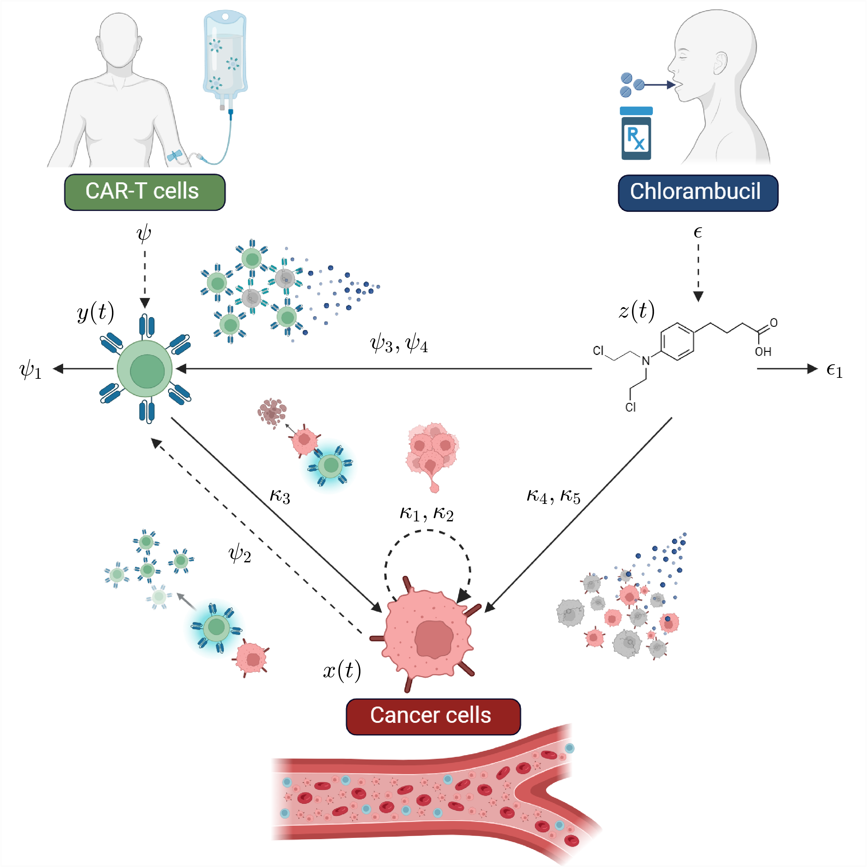
Now, let us describe the system as follows. Equation (1) models the dynamics of CLL cells under the combined treatment of chemoimmunotherapy. The first term describes the development of leukemia cells using a logistic growth law (see Section 4.3 in [15]), which implies a growth rate and a maximum carrying capacity. The second term represents the overall immune response of CAR-T cells against the leukemia cells based on the law of mass action (see Section 2.3 in [16]). The third term accounts for the chemotherapy effect through a pharmacodynamics of maximum response [17]. In the scope of our model, CAR-T cells immunotherapy is considered as the primary treatment strategy, hence, we assume an eradication of cancer cells that follows the log-kill hypothesis [18], i.e., each consecutive application of the treatment should eradicate a fraction of leukemia cells regardless of its total concentration. Chlorambucil drug is used as a secondary treatment, therefore, its cytotoxicity on the leukemia cells is modeled by the Michaelis-Menten kinetics [19]. Equation (2) models the overall behavior of CAR-T cells . The first term accounts for the external application of the effector cells, while the second term captures their natural death. The third term describes activation and proliferation of CAR-T cells upon interaction with leukemia cells in the bloodstream. The fourth term reflects the cytotoxic effect of the chlorambucil drug on CAR-T cells when both therapies are administered into the system at simultaneous periods of time. Equation (3) models the pharmacokinetics of chlorambucil as a first-order process measured in . The first term represents the external administration of the chemotherapy, while the second term accounts for its natural decay over time [20]. The schematic representation of the system is illustrated in Figure 1.
Concerning the overall dynamics, one may apply the positivity property for nonlinear systems established by De Leenheer & Aeyels in [21] and conclude the following:
Remark 1.
Positive system. All forward solutions of the system are nonnegative, and all semi-trajectories of Equations (1)–(3) will be positively forward invariant for nonnegative initial conditions inside the following orthant :
Now, let us consider the cell eradication threshold assumption proposed in [22] which states: “If a solution describing the growth of a cell population goes below the value of 1 cell, then it is possible to assume the complete eradication of such population”. This leads to following remark:
Remark 2.
Clinically significant biological behavior. All solutions for the CLL cells, , and CAR-T cells, , will exhibit biologically meaningful dynamics if their populations persist above the value of 1 cell. Otherwise, one can assume complete eradication. Hence,
and
These remarks will be helpful in drawing conclusions from the in silico experimentation results. First, it is essential to recognize that with positive initial conditions, representing biologically feasible cell and drug concentrations, all solutions will remain within the nonnegative orthant . Additionally, Remark 2 offers a practical threshold to assess cell eradication, emphasizing the interplay between nonlinear systems theory and oncology in the context of a mathematical model describing the combined application of chemotherapy and immunotherapy treatments.
2.2. Parameter Estimation
Altough system (1)–(3) was formulated based on a set of well-established assumptions from the mathematical oncology literature, the values for each parameter were carefully selected or estimated to accurately represent tumor dynamics within the bloodstream of the human body.
First, let us discuss parameters from Equation (1) which models the dynamics of CLL cells . The leukemia cells growth rate, , was derived from the experimental validation perform by Guzev et al. in [23], authors determined the growth rate of A20 murine leukemic cells to be , which, when converted to days, yields a value of . It should be noted that this rate was estimated from cells isolated in vitro, i.e., without the influence of the immune response or therapeutic interventions. Additionally, in vivo studies conducted by the authors estimated a lower growth rate of [24]. A20 cells have been widely used to study the tumor microenvironment in different tissues such as the spleen, brain, and eyes [25], as well as their ability to infiltrate other organs like the liver, lungs, spleen, and bone marrow [26]. Hence, the growth rate of CLL cancer cells can be defined within the following interval:
The maximum leukemia cells carrying capacity, , is derived as follows. Previous studies have estimated around of immune cells in the human body [27,28]. Among these, four main lymphocyte types can be considered: T cells, B cells, NK cells, and plasma cells. According to Sender et al. [27], the total number of B cells is estimated to be with a confidence interval of . Therefore, we set the value of as follows:
Porter et al. published a case report in [29] for a clinical trial involving a patient diagnosed with stage I CLL. In this trial, they designed a lentiviral vector expressing a CAR specific to the B cell antigen CD19. Some key results include the following: CAR-T cells expanded to over times the initial level in vivo; complete remission was achieved and sustained for at least 10 months post-treatment; CAR-T cells persisted at high levels in both the blood and bone marrow for 6 months; a more than 3-log expansion of CAR-T cells was observed by day 21 post-infusion; the doubling time of CAR-T cells in the blood was approximately days, with an elimination half-life of 31 days. Assuming an exponential decay, the death rate of CAR-T cells, , is estimated as follows:
Similarly, the decay rate of the chlorambucil drug, , which has a half-life of hours [30], is calculated as:
Regarding the activation rate of CAR-T cells due to encounters with CLL cells, , our mathematical analysis (discussed further in the next section) leads to the following conclusion:
Remark 3.
Persistence of CAR-T cells.Long-term persistence of CAR-T cells in the system (1)–(3) is ensured if and only if the following condition is satisfied:
otherwise, in the absence of continuous immunotherapy administration, these cells will eventually be depleted.
Therefore, to fulfill condition (4), the value for the activation rate of CAR-T cells is set to at least in order to illustrate CAR-T cells persistence in the in silico experimentation. Now, concerning the cytotoxicity effect of both CAR-T cells and chlorambucil on leukemia cells, we have formulated the following two equations, recently published in [31]:
with
where represents the chlorambucil concentration in , and the values of the parameters for Equations (5)–(5) are provided below in Table 2.
Hence, by substituting the corresponding values for and , the value of may be approximated as follows for both the minimum and maximum growth rate of CLL cells:
The values for the cytotoxicity rate of the chemotherapy on CLL cells, , will be further discussed in the in silico experimentation section, as different concentrations of the chlorambucil drug will be used in the protocol administration design, and results from Guzev et al. [23] indicate that cytotoxicity increases when higher doses of the drug are applied, i.e., greater cell growth inhibition. However, as indicated in off-label dosing guidelines [32,33], total concentrations values should be set within the following range:
for up to 24 cycles. Furthermore, as it has been vastly established in the mathematical oncology literature [19,34], the chemotherapy drug should exhibit a greater capacity for killing cancer cells than effector cells for the treatment to be successful. The latter is to be expected as cancer cells proliferate at a much faster rate than effector cells, hence, the drug must be more effective in killing these malignant cells than healthy or immune cells. Therefore, we set the following constraint for the chlorambucil cytotoxicity rate on CAR-T cells, :
and by following results from de Pillis et al. [19] we set .
Now, concerning the chlorambucil concentration that produces of the maximum response, , we found an in vivo study conducted by Silber et al. [35], in which the chemosensitivity of lymphocytes from patients with B-cell CLL to chlorambucil was determined. The study involved 65 patients diagnosed with CLL, each with at least of monoclonal B lymphocytes positive for CD5, CD19, and CD20 markers. The overall results are summarized as follows: The median for the total patient group was 61 . This value was used as a threshold to categorize the B lymphocytes as sensitive or resistant . Therefore, the value of can be calculated in as L, where the molecular weight of chlorambucil is [36]:
For the concentration of chlorambucil that produces of the maximum cytotoxicity on CAR-T cells, , we follow the same line of thougth as in condition (7) and establish the next condition:
based on the assumption that a higher dose of the chemotherapy drug is required to achieve greater cytotoxicity in CAR-T cells. Similar results were reported by Guzev et al. [24].
3. Results: Nonlinear Dynamical Properties of the System
In this section, we investigate local and global dynamics of Equations (1)–(3) by applying nonlinear system theories such as the Localization of Compact Invariant Sets (LCIS) method to determine lower and upper bounds on all forward solutions of the CLL mechanistic model; Lyapunov’s direct and indirect methods to establish sufficient conditions for eradication of leukemia cells and persistence in both CAR-T cells and cancer cells; and Lipchitz conditions for existence and uniqueness of solutions. Fundamentals and mathematical preliminaries are shown in Appendix A.
3.1. Localizing Domain
The localizing domain containing all compact invariant sets of the system characterizes all biologically meaningful behaviors that may emerge during tumor evolution, such as various concentrations of long-persisting tumor burdens, tumor-free states, periods of cancer cells dormancy followed by heightened effector cells activity, and active immune responses exhibiting abrupt changes in effector and cancer cell concentrations, among other dynamics. Now, by following the LCIS methodology one can establish the next result:
Result I: Clinically significant bounds.
Bounds regarding all compact invariant sets of the CLL system (1)–(3) describing clinically significant behavior when applying either single or combined therapy are given within the next domain:
where each set is defined as follows:
and expressions for the lower and upper bounds of CAR-T cells and CLL cells populations are defined with respect to therapy administration cases as shown below:
| Chemotherapy off | Chemotherapy on |
| where |
| Immunotherapy | Chemotherapy | Chemoimmunotherapy |
Proof.
Now, in order to demonstrate Result I , we first compute the bounds concerning all forward solutions by integrating Equation (3) with the initial condition as follows:
where it is evident that
which also represents the equilibrium point for the constant infusion of the drug into the system. Now, bounds for may be defined as shown below
from which different cases should be considered regarding the initial condition:
- Case 1:.
- In this case chemotherapy is not considered at the beginning of the treatment, therefore:
- Case 2:.
- In this case, bounds are given as follows:
- Case 3: .
- In this case, bounds are defined as follows:
- Case 4: .
- In this case, the initial condition is given by the chemotherapy dose. Thus, when considering parameter values, bounds are given by:
Here, it is important to note that in all numerical simulations, only Case 1 arises, as chemotherapy is not administered as the initial treatment in the designed protocols. These bounds will be necessary to compute lower and upper bounds for both cell’s populations when applying the Iterative Theorem from the LCIS method. First, let us explore the next localizing function:
by computing its Lie derivative
and constructing the set
which is rewritten as follows
from the latter, the lower bound for the CAR-T cells forward solution is given by
where the next two cases should be differentiated
Hence, it is evident that
as it is to be expected because the chemotherapy drug is cytotoxic to both cancer cells and CAR-T cells. Now, an upper bound for the CAR-T cells population may be estimated from the next localizing function:
whose Lie derivative is calculated as
then, set is given below
from the latter, the following condition must be satisfied, implying that the cytotoxic rate of CAR-T cells against cancer cells exceeds the inactivation rate of cancer cells on CAR-T cells,
and set is rewritten as follows
with
and
Therefore, by neglecting the negative function in the right-hand side of the inequality, the next result is obtained
hence, the following upper bound for the CAR-T cells can be extracted
where parameter can have one of the following two values
Now, let us exploit the localizing function:
to derive results concerning the ultimate upper bound for the CAR-T cells in the case of single therapy and combined therapy. Thus, the Lie derivative is computed as follows
then, set is written as given below
Thus, the Iterative Theorem can be applied to determine the following cases concerning single or combined treatment strategies.
- Case 1: Immunotherapy.
- The Iterative Theorem of the LCIS method is applied as follows:and by substituting the corresponding value of Case 1 for the CAR-T cells lower bound one can get the next result:
- Case 2: Chemotherapy.
- When only the chlorambucil drug is being considered, the Iterative Theorem is applied as shown below:and the lower bound is defined as follows
- Case 3: Chemoimmunotherapy.
- Now, let us explore the case when the combined therapy is applied, thus, the Iterative Theorem yields the next result:then, when substituting the corresponding value of Case 2 for the CAR-T cells lower bound the next result can be establish:
Therefore, the proof for Result I is now complete. □
3.2. Eradication Conditions
In this section we establish sufficient conditions by means of Lyapunov’s Direct method to ensure the complete eradication of the CLL cells population described by system (1)–(3). These conditions are formulated on the treatment parameters when considering single and combined application of immunotherapy and chemotherapy. Hence, conditions for CLL cells eradication are given in the next result:
Result II: Minimum concentrations of therapies to ensure a continuous decrease in tumor burden.
If only CAR-T cells are applied, the concentration of this therapy must satisfy the following condition:
On the other hand, if only the chlorambucil drug is appliedand the inequalityholds, then the chemotherapy concentration must fulfill the following condition:
When combined therapy is applied and the concentration of chlorambucil is fixed, the amount of CAR-T cells that needs to be administered into the CLL system (1)–(3) to ensure leukemia cells eradication is given by:
Proof.
Let us apply the next Lyapunov’s candidate function
where it is necessary to highlight that we can explore this function because the lower and upper bounds have already been calculated for both CAR-T cells and the chlorambucil drug in the localizing domain shown in Result I . Thus, inequalities can be constructed on the time-derivative of , which is given as follows:
Therefore, the following three cases can be formulated based on the application of a single therapy or combined therapy.
- Case 1: Immunotherapy.
- When only the CAR-T cells are applied for cancer treatment the time-derivative can be bounded from above as follows:where , and the next constraint can be formulated on the immunotherapy concentration:
- Case 2: Chemotherapy.
- When only the chlorambucil drug is being considered from the beginning of the treatment the time-derivative is bounded from above as indicated below:where as , and the next constraint is formulated on the chemotherapy concentrationhowever, it is evident from the denominator that the next condition relating the rates of CLL cells growth and cytotoxicity of the drug should be fulfilled:or else, condition (12) will not have a biologically feasible solution.
- Case 3: Chemoimmunotherapy.
- When the combined therapy is applied the time-derivative is bounded as follows:where . In order to properly solve this condition, we set the CAR-T cells as the control therapy and come to the following result:in this case it is important to consider two paths. If condition (13) is satisfied, chemotherapy alone could eradicate the leukemia cells population described by the CLL mechanistic model (1)–(3). However, both therapies may be combined in varying proportions to design a successful protocol that ultimately achieves cancer eradication. Conversely, if condition (13) is not fulfilled, then a biologically feasible solution can be computed to estimate the concentration of CAR-T cells required to ensure the complete eradication of cancer cells in the corresponding scenarios.
Therefore, the proof for Result II is now complete. □
3.3. Persistence Conditions
In order to derive results regarding the so-called persistence conditions for both CLL cells and CAR-T cells, we compute the core equilibrium points of system (1)–(3) by excluding the therapy parameters and setting the equations to zero as follows:
It should be noted that treatments are not considered because, in real-life clinical scenarios, anti-cancer therapies are administered in short cycles over limited periods of time. The latter, within the scope of nonlinear system theory, are referred to as perturbations and their primary characteristic is their ability to alter both the short- and long-term dynamics of a system. These changes may be minor, disrupting only short-term behavior, or major, affecting long-term dynamics and transitioning the system through completely different states. Hence, by performing the corresponding arithmetical operations, the following three sets of equilibrium points are identified:
Now, let us discuss the biological interpretation of each equilibrium point. Equilibrium (15) corresponds to the tumor-free state, representing the desired outcome after a successful treatment strategy that eradicates the CLL cells population. Concerning equilibrium (16), we can see that it is biologically feasible if the persistence condition (4) from Remark 3 is satisfied. Furthermore, positive values are required to describe real-life cells concentrations. This equilibrium represents a state where CAR-T cells persist in the long-term, enabling them to mount a consistent immune response against cancer cells, thereby reducing the tumor burden in the system to a value directly related to the ratio . Equilibrium (17) represents a scenario in which leukemia cells reach their maximum carrying capacity. Within the framework of system (1)–(3) this implies the death of the subject, as the tumor burden becomes unsustainable for survival. Now, let us present the following result regarding the long-term concentration of cells populations:
Result III: Persistence and depletion of CAR-T cells.
If condition (4) from Remark III is satisfied, i.e.,
CAR-T cells will persist in the long-term after a single application of the therapy. Under this condition, cell populations will reach the following steady-state concentrations where both coexist:
However, if condition (4) is not satisfied, CAR-T cells will eventually be depleted, and CLL cells will grow to their maximum carrying capacity, i.e.,
Proof.
Local dynamics of the CLL mechanistic model can be explored by applying the Indirect Lyapunov’s method which requires the Jacobian matrix of the system which is computed as follows:
From the latter, one can determine the corresponding eigenvalues to each equilibrium point as indicated in the cases below.
- Case 1: Equilibrium
-
The Jacobian matrix has the following form:Hence, it is evident that this equilibrium is unstable, as one of the eigenvalues is positive,This outcome is to be expected, as once cancer cells evade the immune response, either by suppressing the immune system or by remaining undetected by effector cells, they will grow to their maximum carrying capacity or to the extent that the subject can endure. This scenario also indicates that treatment strategies were either unsuccessful or not administered.
- Case 2: Equilibrium
-
The Jacobian matrix evaluated at this equilibrium point is given by:with the next eigenvalues:It is evident that the radicands in and will be positive and real if the persistence condition (4) from Remark III holds, i.e., ,which allows us to conclude that equilibrium (16) is locally asymptotically stable. Conversely, if condition (4) is not satisfied, equilibrium (16) becomes unstable and biologically infeasible, as . In this case, if therapies are unsuccessful, cancer cells will grow to their maximum carrying capacity , making (17) the only locally asymptotically stable equilibrium point of the system as it is shown in the next case.
- Case 3: Equilibrium
-
The Jacobian matrix is upper triangular, as shown below:Therefore, the eigenvalues correspond to the diagonal elements of the matrix:From these results, two scenarios are identified. First, equilibrium point (17) is locally asymptotically stable ifThis indicates that the persistence condition (4) from Remark III is not satisfied. In this case, long-term persistence of CAR-T cells cannot be expected, as equilibrium (16) does not exist within the positive and biologically feasible domain of the system. Nonetheless, if the persistence condition (4) is satisfied, equilibrium (17) becomes unstable, and the only locally asymptotically stable equilibrium point is (16). This implies that both cell populations described by the CLL mechanistic model (1)–(3) coexist. However, the in silico experimentation will reveal whether this sustained immune response by the CAR-T cells is sufficient to reduce the tumor burden to a level that is manageable for the subject’s health. Results from these three cases allows us to conclude that if the chemoimmunotherapy treatment strategy is not successful, leukemia cells will always persist.
Therefore, the proof for Result III is now complete. □
3.4. Existence and Uniqueness
A system of first-order nonlinear ODEs may exhibit multiple solutions for a given set of initial conditions. This ambiguity poses significant challenges when modeling specific scenarios in tumor-immune dynamics, as these dynamics are intrinsically linked to particular conditions and parameter values. However, based on the results presented in this section, we establish the following conclusions regarding the existence and uniqueness of solutions for the CLL system (1)–(3) proposed in this work:
Result IV: Ensuring a reliablein silicoexperimentation for tumor-immune dynamics. Let vector fields, where, be piecewise continuous intand locally Lipchitz infor alland allin. Since every solution of the system (1)–(3), with initial conditions, remains entirely within, there exist a unique solution defined for all
.
Proof.
First, note that vector fields of system (1)–(3) are given by
where all elements are continuous in by Remark I , i.e., , and piecewise continuous in t. This is crucial because therapies are considered perturbations, applied as impulse changes in short cycles over limited periods of time. Furthermore, one can see that all components of the Jacobian Matrix (18) are also piecewise continuous in t and bounded within the domain , as established by Results I and II . Consequently, is locally Lipchitz in in the domain , where , as there exists a Lipschitz constant such that
on , and satisfies the Lipchitz condition:
Therefore, the proof for Result IV is now complete. □
4. Discussion: In Silico Experimentation
In this section, we explore the global dynamics of our mechanistic model (1)–(3) as well as its capabilities to investigate different scenarios of tumor-immune dynamics through in silico experimentation. First, Figure 2 illustrates outcomes related to condition (4) from Result III , and the eradication condition (11) from Result II through the following three cases:
- Case 1: Depletion of CAR-T cells.
- Depletion of CAR-T cells in the short-term happens when condition (4) is not satisfied. As expected, the concentration of CLL cells grows to their maximum carrying capacity, while CAR-T cells eventually fall below the threshold of clinically significant biological behavior, defined as fewer than 1 cell. Hence, solutions go to the equilibrium point (17), i.e, . For the sake of numerical simulations, dynamics are simulated following a single application of the therapy under the next set of initial conditions: CLL cells, CAR-T cells (unique dose), and mg of chlorambucil. Parameter values are as follows: , , , , . Other parameters are set as zero, as chemotherapy is not considered in this scenario. Results for this in silico experimentation are shown in the top panels of Figure 2.
- Case 2: Persistence of CAR-T cells.
- Long-term persistence of CAR-T cells is observed when condition (4) is fulfilled. In this case, cells concentrations stabilize at a steady-state defined by the equilibrium point (16) . However, this outcome does not represent a viable treatment strategy for real-world clinical scenarios, because the tumor burden remains near the maximum carrying capacity. For the sake of numerical simulations, dynamics are simulated following a single application of the therapy under the next set of initial conditions: CLL cells, CAR-T cells (unique dose), and mg of chlorambucil. Parameter values are as follows: , , , , . Other parameters are set as zero, as chemotherapy is not considered in this scenario. Results for this in silico experimentation are shown in the middle panels of Figure 2.
- Case 3: Eradication of CLL cells.
- Within the scope of system (1)–(3), eradication of CLL cells is ensured when the concentration of CAR-T cells meets condition (11). Hence, the immunotherapy control parameter is set with a constant value of which equals to cells. Dynamics are simulated following a constant application of the therapy under the next set of initial conditions: CLL cells, CAR-T cells (constant dose), and mg of chlorambucil. Parameter values are as follows: , , , , . Other parameters are set as zero, as chemotherapy is not considered in this scenario. Results for this in silico experimentation are shown in the bottom panels of Figure 2.
All chemoimmunotherapy protocols explored in this work are designed under the next assumptions: CAR-T cells will persist in the long-term after infusion into the subject as it was described in Case 2 of Figure 2, i.e, ; CLL cells display the highest growth rate, i.e, and are resistant to the chemotherapy drug, i.e., .
Hence, let us explore the dose-escalation scheme often employed in phase I clinical trials for cancer patients treated with T-cell therapies [37,38,39,40,41]. In such protocols, dose levels are typically defined as an absolute number of cells, ranging from to cells, or as dose normalized to the patient’s body weight, which may range from up to a maximum dose of . It is important to note that dosing regimens can vary between studies, with the optimal dose typically determined through careful escalation in clinical trials to balance efficacy and safety. However, this falls outside the scope of the present research, as the focus is on in silico experimentation rather than in vivo studies. Hence, after extensive iterations of numerical simulations, the scheme of Table 3 was designed using an algorithm developed in MATLAB.
This protocol aims to eliminate CLL cells concentrations under varying initial tumor burden scenarios, defined as leukemia cells, for . For the purposes of the in silicoexperimentation, the maximum initial tumor burden considered represents approximately of the system’s estimated carrying capacity. Results are illustrated in Figure 3, the top panel corresponds to the CLL cells , demonstrating the combined effects of the CAR-T cells and chlorambucil doses over time. It is evident that, under the same protocol scheme, a lower initial concentration of leukemia cells is eradicated in a shorter period of time. Panels in the middle row depict the behavior of CAR-T cells and the chlorambucil drug in the bloodstream compartment, whereas panels in the bottom row illustrate the dose-escalation protocol. It should be noted that each dose of CAR-T cells satisfies conditions outlined in Result II , particularly condition (11) as the therapies are administered sequentially without overlapping. Chlorambucil doses were calculated based on the median weight of an adult CLL patient, estimated to be 81 [42,43], and drug cytotoxicity on both CLL and CAR-T cells changes for each dose concentration as indicated in Table 4.
Now, following nonlinear dynamical systems theory, we can expect that an initial higher dose of CAR-T cells will have a more significant and long-term effect on the overall behavior of the system. Using our algorithm, a dose de-escalation protocol was designed with the characteristics shown in Table 5.
Results are illustrated in Figure 4, where the arrangement of solutions, i.e., cells and drug concentrations dynamics as well as protocols, is consistent with that in Figure 3. Nonetheless, there are some key differences that should be discussed. First, the dose-escalation protocol required a total of CAR-T cells to completely eradicate the highest concentration of CLL cells, i.e., cells. In contrast, the dose de-escalation scheme achieved leukemia eradication with a total of CAR-T cells. Numerical simulations indicate that in the dose-escalation protocol, CLL cell growth still occurs after the first dose of immunotherapy, as the initial lower concentration of CAR-T cells is insufficient to mount a successful immune response against cancer, even at lower tumor burdens. However, the dose de-escalation protocol demonstrates a consistent reduction in CLL cell concentrations starting from the first dose. Furthermore, the highest dose in the protocol falls within the previously stated range, with CAR-T cells administered in the first dose. However, assessing the maximum tolerated dose lies beyond the scope of this in silico experimentation. Additionally, it should be noted that the effects of the chemotherapy drug on CLL cell concentrations are not perceptible in Figure 3 and Figure 4 because numerical simulations are performed under two key assumptions. First, the leukemia cells are assumed to exhibit drug resistance, and second, condition (13) is not satisfied, as the growth rate of leukemia cells is deliberately set to its highest value.
While protocol failure is undesirable in cancer treatment, a significant proportion of phase I clinical trials encounter such outcomes [41,44,45]. Therefore, we illustrate in Figure 5 and Figure 6 tumor escape in both dose-escalation and dose de-escalation schemes, respectively, emphasizing that any protocol may fail if doses are not accurately calculated, and cancer cell concentrations are not consistently monitored. Parameter values are the same as the successful protocols, i.e., , , , , , , , . It is important to note that the CAR-T doses were determined heuristically, aiming for a solution that approaches the threshold of 1 cancer cell, as established in Remark 2 for clinically significant biological behavior.
In silico experiments presented in this section were performed on a computer with the following specifications: Ryzen 9 7950X CPU, 192 GB DDR5 CL40 RAM, and a 1 TB Samsung 990 Pro Gen 4 NVMe M.2 drive. The algorithm used for these experiments, designed in MATLAB, is available as supplementary material in a GitHub repository, and certified under INDAUTOR registration number 03-2023-052912465900-01.
5. Conclusions
In this work, we proposed a mechanistic nonlinear model to study the dynamics of CLL under combined chemoimmunotherapy. The model consists of a system of three first-order ODEs that describe the effects of CAR-T cells and chlorambucil on the leukemia cells population over both short- and long-term timescales. Using a model-based design approach and extensive in silico experimentation, we determined sufficient dosing strategies for each therapeutic application. The local and global dynamics of model (1)–(3) were thoroughly analyzed using various nonlinear systems theories. Consequently, we derived conditions to ensure the eradication of cancer cells, with numerical simulations illustrating that the population falls below the threshold for clinically significant biological behavior, defined as one cell.
Furthermore, our algorithm enables the exploration of different scenarios. As illustrated, we compared two chemoimmunotherapy application protocols: dose-escalation and dose de-escalation. While dose-escalation protocols are commonly used in Phase I trials, numerical simulations suggest that the dose de-escalation protocol may require a lower total dose to achieve effective tumor-immune dynamics, as a higher initial dose tends to have a greater impact. However, in silico experiments also show that, even with complete remission (peripheral blood lymphocytes count ) or partial remission (a decrease in the number of blood lymphocytes to or less from the value before therapy) [46], relapse can occur if the dosing is insufficient or if therapy is administered without ensuring the eradication of minimal residual disease.
Nonetheless, for any model-based design approach to be successful in dose-finding for anti-cancer therapies, one open problem remains: all parameters of a mathematical model, such as the one proposed in this work, must be carefully estimated for each patient. Therefore, clinical data on cancer cell growth rates, CAR-T cell activation rates, and the cytotoxicity rates of therapies are crucial values for protocol dosing design from the perspective of nonlinear dynamical systems and in silico experimentation. Finally, our algorithm could be useful for estimating key parameters through nonlinear regression functions in the MATLAB environment when tumor-immune dynamics data, in the form of cell counts over time, are available for a given patient.
Author Contributions
Conceptualization, P.A.V. and L.N.C.; methodology, C.P. and Y.S.; software, P.A.V. and L.A.R.; validation, C.P. and L.N.C.; formal analysis, P.A.V.; investigation, L.N.C. and Y.S.; resources, P.A.V. and L.N.C.; writing—original draft preparation, P.A.V. and L.N.C.; writing—review and editing, Y.S., L.A.R. and C.P.; visualisation, P.A.V. and L.N.C.; project administration, P.A.V.; funding acquisition P.A.V. and L.N.C. All authors have read and agreed to the published version of the manuscript.
Funding
This research was funded by the TecNM grants “Estrategias in silico integradas con biomatemáticas y sistemas dinámicos no lineales para el modelizado, análisis y control de sistemas biológicos: Parte II”, “Modelizado de sistemas no lineales para procesos de fermentación basados en la dinámica de crecimiento de microorganismos: parte 3 ”, and PENDING...
Institutional Review Board Statement
Not applicable
Data Availability Statement
The algorithm design for the in silico experiments performed in this work was developed in MATLAB, it is available as supplementary material in a GitHub repository, and certified under INDAUTOR registration number 03-2023-052912465900-01.
Acknowledgments
This research was fulfilled within the academic research group “Sistemas dinámicos no lineales (ITIJ-CA-10)”, and the “Red Internacional de Control y Cómputo Aplicados (RICCA)”.
Conflicts of Interest
The authors declare no conflicts of interest.
Appendix A. Notations and Mathematical Foundations
Nonlinear dynamical systems considered in this work are of the form:
These are referred to as time-variant systems, where is continuous in and piecewise continuous in t. Consequently, solutions can only be piecewise continuously differentiable. This assumption enables the inclusion of cases where depends on a time-varying input, such as step functions or finite impulses. However, if the system (A1) does not depend explicitly on t, or the input is constant, then the system reduces to the following form:
Here, is a continuously differentiable vector function and represents the state vector. Systems of this type are called time-invariant.
Appendix A.1. Positiveness of Solutions
Consider a nonlinear dynamical system of the form (A2), which is called positive, P, if the nonnegative orthant is forward invariant. This implies that for any initial condition at , the forward solution for all . The boundary of the nonnegative orthant is denoted as and consists of all points x where at least one component of x is zero, i.e., for some and for all . Hence, the following Lemma provides a sufficient and necessary condition to establish positivity of system (A2), as detailed in Section in [21]:
Lemma A1.
Positiveness of solutions. The nonlinear system is positive if and only if the following condition holds:
This condition ensures that the vector field does not point out of at its boundary . Therefore, given nonnegative initial conditions, all solutions will remain within for all .
Appendix A.2. Localization of Compact Invariant Sets Method
The Localization of Compact Invariant Sets (LCIS) method [47,48] was formulated to study the long-term dynamics of nonlinear systems of first-order ODEs. Examples of compact invariant sets are the following: equilibrium points; periodic, homoclinic, and heteroclinic orbits; limit cycles, and chaotic attractors. The General Theorem is written as follows for a system of the form (A1), as detailed in Section 2 in [49]:
Theorem A1.
General theorem. Each compact invariant set Γ of is contained in the localizing domain:
In order to apply the LCIS method, first one should propose the so-called localizing function , , which is defined on the space , and it is assumed that is not the first integral of (A1). Further, denotes the restriction of on a set . Thus, denotes the set , where represents the Lie derivative (temporal derivative) of and it is given by . From the latter, one can define and . Now, a refinement of Theorem A1 is realized with help of the Iterative theorem stated as follows:
Theorem A2.
Iterative theorem. Let be a sequence of differentiable functions. Sets
with
contain any compact invariant set of the system and
The distinctiveness of the LCIS method lies in its strictly analytical nature, enabling the solution of the problem without solving the system of ODEs.
Appendix A.3. Stability in the Sense of Lyapunov
Lyapunov demonstrated that certain types of functions, called Lyapunov candidate functions, can be used to investigate the stability of the equilibrium point of a nonlinear system of the form (A2). A Lyapunov candidate function must satisfy the following properties:
- Positive definiteness: and for all .
- Radial unboundedness: as .
The temporal derivative of along the trajectories of the system is given by , where is a negative definite function if and for all . Thus, the Theorem of global asymptotic stability in the sense of Lyapunov is formulated as below, as detailed in Section in [50] and Chapter 2 in [51]:
Theorem A3.
Lyapunov’s direct method.The equilibrium point of is globally asymptotically stable if there exists a positive definite and radially unbounded function such that is negative definite.
A function that satisfies the properties of this theorem is called a Lyapunov function. However, there is no explicit method to find a candidate, and they should be formulated by trial and error. It is also important to note that the failure of a Lyapunov candidate function to satisfy the conditions of Theorem A3 does not necessarily imply that the equilibrium is unstable. It only indicates that stability in the sense of Lyapunov cannot be established with the chosen candidate.
In a small neighborhood of the origin, a nonlinear system of the form (A2) can be approximated by its linearization about this point:
The following theorem provides conditions under which the stability of the origin for the nonlinear system (A2) can be inferred from the stability of the linearized system, as detailed in Section 4.3 in [50]:
Theorem A4.
Lyapunov’s indirect method. Let the equilibrium point of where is continuously differentiable and D is a neighborhood of the origin. Then:
- The origin is asymptotically stable if all eigenvalues of A satisfy .
- The origin is unstable if one or more eigenvalues of Asatisfy .
Appendix A.4. Lipschitz Condition
In order to predict the future state of a system described by a nonlinear dynamical system of the form (A1) from its present state at , the initial value problem:
must have a unique solution. The existence and uniqueness of such a solution can be guaranteed by imposing a constraint on the right-hand side function , known as the Lipschitz condition. This condition requires to satisfy the inequality:
for all and in some neighborhood of , where ℓ is the Lipschitz constant. The following results, detailed in Section 3.1 of [50], provide further insight into the Lipschitz condition:
Lemma A2.
Locally Lipschitz. If and are continuous on , with for some domain , then f is locally Lipschitz in x on .
Theorem A5.
Existence and uniqueness. Let be piecewise continuous in t and locally Lipschitz in x for all and x in a domain . Let K be a compact subset of D, , and suppose it is known that every solution of , lies entirely in K. Then, there exists a unique solution defined for al .
The key challenge in applying Theorem A5 lies in verifying that every solution remains within a compact domain K without explicitly solving the system of ODEs.
References
- Yao, Y.; Lin, X.; Li, F.; Jin, J.; Wang, H. The global burden and attributable risk factors of chronic lymphocytic leukemia in 204 countries and territories from 1990 to 2019: analysis based on the global burden of disease study 2019. BioMedical Engineering OnLine 2022, 21. [Google Scholar] [CrossRef] [PubMed]
- Ghia, P.; Ferreri, A.J.; Caligaris-Cappio, F. Chronic lymphocytic leukemia. Critical Reviews in Oncology/Hematology 2007, 64, 234–246. [Google Scholar] [CrossRef] [PubMed]
- Burger, J.A.; O’Brien, S. Evolution of CLL treatment — from chemoimmunotherapy to targeted and individualized therapy. Nature Reviews Clinical Oncology 2018, 15, 510–527. [Google Scholar] [CrossRef]
- Sun, D.; Shi, X.; Li, S.; Wang, X.; Yang, X.; Wan, M. CAR-T cell therapy: A breakthrough in traditional cancer treatment strategies (Review). Molecular Medicine Reports 2024, 29. [Google Scholar] [CrossRef] [PubMed]
- Borogovac, A.; Siddiqi, T. Advancing CAR T-cell therapy for chronic lymphocytic leukemia: exploring resistance mechanisms and the innovative strategies to overcome them. Cancer Drug Resistance 2024. [Google Scholar] [CrossRef]
- Hallek, M. Chronic lymphocytic leukemia: 2020 update on diagnosis, risk stratification and treatment. American Journal of Hematology 2019, 94, 1266–1287. [Google Scholar] [CrossRef]
- Brady, R.; Enderling, H. Mathematical Models of Cancer: When to Predict Novel Therapies, and When Not to. Bulletin of Mathematical Biology 2019, 81, 3722–3731. [Google Scholar] [CrossRef]
- Malinzi, J.; Basita, K.B.; Padidar, S.; Adeola, H.A. Prospect for application of mathematical models in combination cancer treatments. Informatics in Medicine Unlocked 2021, 23, 100534. [Google Scholar] [CrossRef]
- Joslyn, L.R.; Huang, W.; Miles, D.; Hosseini, I.; Ramanujan, S. Digital twins elucidate critical role of Tscm in clinical persistence of TCR-engineered cell therapy. npj Systems Biology and Applications 2024, 10. [Google Scholar] [CrossRef]
- Huang, X.; Li, Y.; Zhang, J.; Yan, L.; Zhao, H.; Ding, L.; Bhatara, S.; Yang, X.; Yoshimura, S.; Yang, W.; et al. Single-cell systems pharmacology identifies development-driven drug response and combination therapy in B cell acute lymphoblastic leukemia. Cancer Cell 2024, 42, 552–567.e6. [Google Scholar] [CrossRef]
- Love, S.B.; Brown, S.; Weir, C.J.; Harbron, C.; Yap, C.; Gaschler-Markefski, B.; Matcham, J.; Caffrey, L.; McKevitt, C.; Clive, S.; et al. Embracing model-based designs for dose-finding trials. British journal of cancer 2017, 117, 332–339. [Google Scholar] [CrossRef] [PubMed]
- Belov, A.; Schultz, K.; Forshee, R.; Tegenge, M.A. Opportunities and challenges for applying model-informed drug development approaches to gene therapies. CPT: Pharmacometrics & Systems Pharmacology 2021, 10, 286–290. [Google Scholar] [CrossRef]
- Chelliah, V.; Lazarou, G.; Bhatnagar, S.; Gibbs, J.P.; Nijsen, M.; Ray, A.; Stoll, B.; Thompson, R.A.; Gulati, A.; Soukharev, S.; et al. Quantitative systems pharmacology approaches for immuno-oncology: adding virtual patients to the development paradigm. Clinical Pharmacology & Therapeutics 2021, 109, 605–618. [Google Scholar] [CrossRef]
- Milo, R.; Phillips, R. Cell biology by the numbers; Garland Science: New York, New York, USA, 2015. [Google Scholar]
- Dominik, W.; Natalia, K. Dynamics of cancer: mathematical foundations of oncology; World Scientific: Hackensack, New Jersey, USA, 2014. [Google Scholar]
- Britton, N.F. Essential mathematical biology; Springer Science & Business Media: New York, New York, USA, 2012. [Google Scholar] [CrossRef]
- Holford, N. Pharmacodynamic principles and the time course of immediate drug effects. Translational and clinical pharmacology 2017, 25, 157–161. [Google Scholar] [CrossRef]
- Norton, L. Cancer log-kill revisited. American Society of Clinical Oncology Educational Book 2014, 34, 3–7. [Google Scholar] [CrossRef]
- de Pillis, L.; Fister, K.R.; Gu, W.; Collins, C.; Daub, M.; Gross, D.; Moore, J.; Preskill, B. Mathematical model creation for cancer chemo-immunotherapy. Computational and Mathematical Methods in Medicine 2009, 10, 165–184. [Google Scholar] [CrossRef]
- Byers, J.P.; Sarver, J.G. Pharmacokinetic modeling. In Pharmacology; Elsevier: New York, New York, USA, 2009; pp. 201–277. [Google Scholar] [CrossRef]
- De Leenheer, P.; Aeyels, D. Stability properties of equilibria of classes of cooperative systems. IEEE Transactions on Automatic Control 2001, 46, 1996–2001. [Google Scholar] [CrossRef]
- Valle, P.A.; Coria, L.N.; Plata, C.; Salazar, Y. CAR-T Cell Therapy for the Treatment of ALL: Eradication Conditions and In Silico Experimentation. Hemato 2021, 2, 441–462. [Google Scholar] [CrossRef]
- Guzev, E.; Luboshits, G.; Bunimovich-Mendrazitsky, S.; Firer, M.A. Experimental Validation of a Mathematical Model to Describe the Drug Cytotoxicity of Leukemic Cells. Symmetry 2021, 13, 1760. [Google Scholar] [CrossRef]
- Guzev, E.; Jadhav, S.S.; Hezkiy, E.E.; Sherman, M.Y.; Firer, M.A.; Bunimovich-Mendrazitsky, S. Validation of a Mathematical Model Describing the Dynamics of Chemotherapy for Chronic Lymphocytic Leukemia In Vivo. Cells 2022, 11, 2325. [Google Scholar] [CrossRef]
- Donnou, S.; Galand, C.; Touitou, V.; Sautès-Fridman, C.; Fabry, Z.; Fisson, S. Murine models of B-cell lymphomas: promising tools for designing cancer therapies. Advances in hematology 2012, 2012, 701704. [Google Scholar] [CrossRef] [PubMed]
- Mashima, K.; Azuma, M.; Fujiwara, K.; Inagaki, T.; Oh, I.; Ikeda, T.; Umino, K.; Nakano, H.; Morita, K.; Sato, K.; et al. Differential localization and invasion of tumor cells in mouse models of human and murine leukemias. Acta Histochemica et Cytochemica 2020, 53, 43–53. [Google Scholar] [CrossRef]
- Sender, R.; Weiss, Y.; Navon, Y.; Milo, I.; Azulay, N.; Keren, L.; Fuchs, S.; Ben-Zvi, D.; Noor, E.; Milo, R. The total mass, number, and distribution of immune cells in the human body. Proceedings of the National Academy of Sciences 2023, 120, e2308511120. [Google Scholar] [CrossRef] [PubMed]
- Hatton, I.A.; Galbraith, E.D.; Merleau, N.S.; Miettinen, T.P.; Smith, B.M.; Shander, J.A. The human cell count and size distribution. Proceedings of the National Academy of Sciences 2023, 120, e2303077120. [Google Scholar] [CrossRef] [PubMed]
- Porter, D.L.; Levine, B.L.; Kalos, M.; Bagg, A.; June, C.H. Chimeric antigen receptor–modified T cells in chronic lymphoid leukemia. New England Journal of Medicine 2011, 365, 725–733. [Google Scholar] [CrossRef]
- National Center for Biotechnology Information (2022). PubChem Compound Summary for CID 2708, Chlorambucil. https://pubchem.ncbi.nlm.nih.gov/compound/Chlorambucil, 2024. Updated: September/14/2024.
- Valle, P.A.; Garrido, R.; Salazar, Y.; Coria, L.N.; Plata, C. Chemoimmunotherapy Administration Protocol Design for the Treatment of Leukemia through Mathematical Modeling and In Silico Experimentation. Pharmaceutics 2022, 14, 1396. [Google Scholar] [CrossRef]
- Eichhorst, B.F.; Busch, R.; Stilgenbauer, S.; Stauch, M.; Bergmann, M.A.; Ritgen, M.; Kranzhöfer, N.; Rohrberg, R.; Söling, U.; Burkhard, O.; et al. First-line therapy with fludarabine compared with chlorambucil does not result in a major benefit for elderly patients with advanced chronic lymphocytic leukemia. Blood, The Journal of the American Society of Hematology 2009, 114, 3382–3391. [Google Scholar] [CrossRef]
- Access Pharmacy. Drug Monogrpahs: Chlorambucil. https://accesspharmacy.mhmedical.com/, 2024. Accessed: 01/October/2024.
- de Pillis, L.G.; Gu, W.; Radunskaya, A.E. Mixed immunotherapy and chemotherapy of tumors: modeling, applications and biological interpretations. Journal of theoretical biology 2006, 238, 841–862. [Google Scholar] [CrossRef]
- Silber, R.; Degar, B.; Costin, D.; Newcomb, E.W.; Mani, M.; Rosenberg, C.R.; Morse, L.; Drygas, J.C.; Canellakis, Z.N.; Potmesil, M. Chemosensitivity of lymphocytes from patients with B-cell chronic lymphocytic leukemia to chlorambucil, fludarabine, and camptothecin analogs. Blood 1994, 84, 3440–46. [Google Scholar] [CrossRef]
- Drugbank Online. Chlorambucil. https://go.drugbank.com/drugs/DB00291, 2024. Updated: August/02/2024.
- Lee, D.W.; Kochenderfer, J.N.; Stetler-Stevenson, M.; Cui, Y.K.; Delbrook, C.; Feldman, S.A.; Fry, T.J.; Orentas, R.; Sabatino, M.; Shah, N.N.; et al. T cells expressing CD19 chimeric antigen receptors for acute lymphoblastic leukaemia in children and young adults: a phase 1 dose-escalation trial. Lancet 2015, 385, 517–528. [Google Scholar] [CrossRef]
- Zhang, C.; Wang, Z.; Yang, Z.; Wang, M.; Li, S.; Li, Y.; Zhang, R.; Xiong, Z.; Wei, Z.; Shen, J.; et al. Phase I escalating-dose trial of CAR-T therapy targeting CEA+ metastatic colorectal cancers. Molecular Therapy 2017, 25, 1248–1258. [Google Scholar] [CrossRef] [PubMed]
- George, P.; Dasyam, N.; Giunti, G.; Mester, B.; Bauer, E.; Andrews, B.; Perera, T.; Ostapowicz, T.; Frampton, C.; Li, P.; et al. Third-generation anti-CD19 chimeric antigen receptor T-cells incorporating a TLR2 domain for relapsed or refractory B-cell lymphoma: a phase I clinical trial protocol (ENABLE). BMJ open 2020, 10, e034629. [Google Scholar] [CrossRef] [PubMed]
- Chen, Y.; Zhao, H.; Luo, J.; Liao, Y.; Dan, X.; Hu, G.; Gu, W. A phase I dose-escalation study of neoantigen-activated haploidentical T cell therapy for the treatment of relapsed or refractory peripheral T-cell lymphoma. Frontiers in Oncology 2022, 12, 944511. [Google Scholar] [CrossRef]
- Bulsara, S.; Wu, M.; Wang, T. Phase I CAR-T Clinical Trials Review. Anticancer research 2022, 42, 5673–5684. [Google Scholar] [CrossRef]
- Williams, A.M.; Baran, A.M.; Schaffer, M.; Bushart, J.; Rich, L.; Moore, J.; Barr, P.M.; Zent, C.S. Significant weight gain in CLL patients treated with ibrutinib: a potentially deleterious consequence of therapy. American journal of hematology 2019, 95, E16. [Google Scholar] [CrossRef]
- Sitlinger, A.; Deal, M.A.; Garcia, E.; Thompson, D.K.; Stewart, T.; MacDonald, G.A.; Devos, N.; Corcoran, D.; Staats, J.S.; Enzor, J.; et al. Physiological fitness and the pathophysiology of chronic lymphocytic leukemia (CLL). Cells 2021, 10, 1165. [Google Scholar] [CrossRef]
- Liu, C.; Yang, M.; Zhang, D.; Chen, M.; Zhu, D. Clinical cancer immunotherapy: Current progress and prospects. Frontiers in immunology 2022, 13, 961805. [Google Scholar] [CrossRef]
- Ling, S.P.; Ming, L.C.; Dhaliwal, J.S.; Gupta, M.; Ardianto, C.; Goh, K.W.; Hussain, Z.; Shafqat, N. Role of Immunotherapy in the treatment of cancer: A systematic review. Cancers 2022, 14, 5205. [Google Scholar] [CrossRef]
- Hallek, M.; Cheson, B.D.; Catovsky, D.; Caligaris-Cappio, F.; Dighiero, G.; Döhner, H.; Hillmen, P.; Keating, M.; Montserrat, E.; Chiorazzi, N.; et al. iwCLL guidelines for diagnosis, indications for treatment, response assessment, and supportive management of CLL. Blood, The Journal of the American Society of Hematology 2018, 131, 2745–2760. [Google Scholar] [CrossRef]
- Krishchenko, A.P. Localization of invariant compact sets of dynamical systems. Differ Equ 2005, 41, 1669–1676. [Google Scholar] [CrossRef]
- Krishchenko, A.P.; Starkov, K.E. Localization of compact invariant sets of the Lorenz system. Phys Lett A 2006, 353, 383–388. [Google Scholar] [CrossRef]
- Krishchenko, A.P.; Starkov, K.E. Localization of compact invariant sets of nonlinear time-varying systems. International Journal of Bifurcation and Chaos 2008, 18, 1599–1604. [Google Scholar] [CrossRef]
- Khalil, H.K. Nonlinear systems, 3 ed.; Prentice-Hall: Hoboken, NJ, USA, 2002. [Google Scholar]
- Hahn, W.; Hosenthien, H.H.; Lehnigk, S.H. Theory and application of Liapunov’s direct method; Dover Publications, Inc.: Mineola, NY, USA, 2019. [Google Scholar]
Figure 1.
Schematic diagram of the CLL system illustrating all interactions described by Equations (1)–(3). The diagram includes the administered therapies, the cytotoxic effects of CAR-T cells and chlorambucil on leukemia cells, and the cross-cytotoxicity of the chemotherapy drug on effector cells. Additionally, it highlights the activation of CAR-T cells triggered by interactions with cancer cells and the self-stimulating growth of leukemia cells. Diagram created in BioRender: https://BioRender.com/s31e824.
Figure 2.
In silico experimentation performed to illustrate various tumor-immune dynamics in the absence of chemotherapy. The panels in the top row depict the depletion of CAR-T cells; those in the middle row demonstrate CAR-T cells persistence; and the panels in the bottom row show the eradication of CLL cells when a constant concentration of CAR-T cells is infused into the system. However, none of these cases reflect real-life clinical behavior, but instead represent the local and global dynamics of Equations (1)–(3).
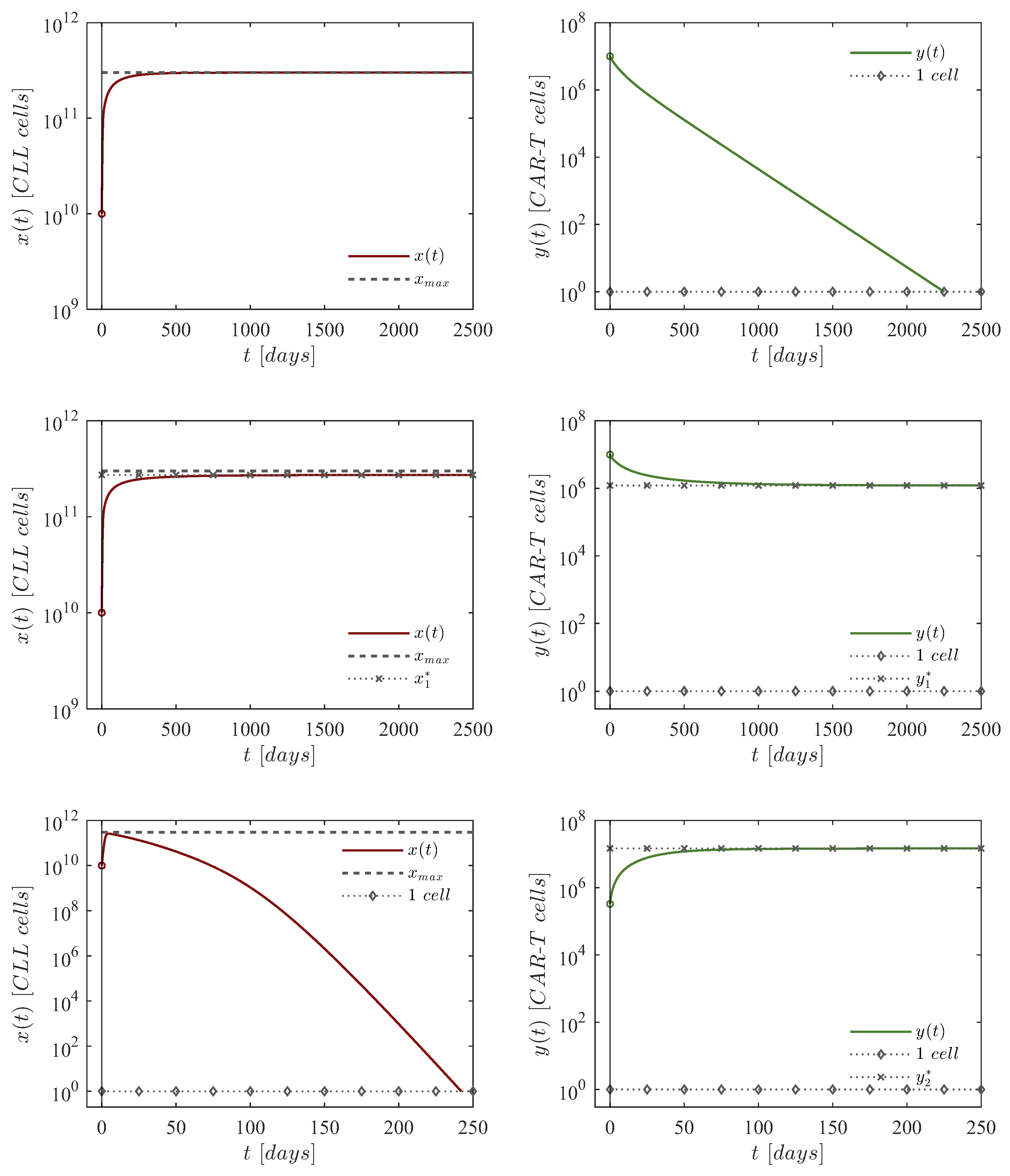
Figure 3.
In silico experimentation for the dose-escalation chemoimmunotherapy protocol for eleven initial CLL cells concentrations. Dynamics are simulated under the next set of initial conditions: CLL cells with , CAR-T cells, and mg of chlorambucil. Parameter values are as follows: , , , , , , ,
Figure 3.
In silico experimentation for the dose-escalation chemoimmunotherapy protocol for eleven initial CLL cells concentrations. Dynamics are simulated under the next set of initial conditions: CLL cells with , CAR-T cells, and mg of chlorambucil. Parameter values are as follows: , , , , , , ,
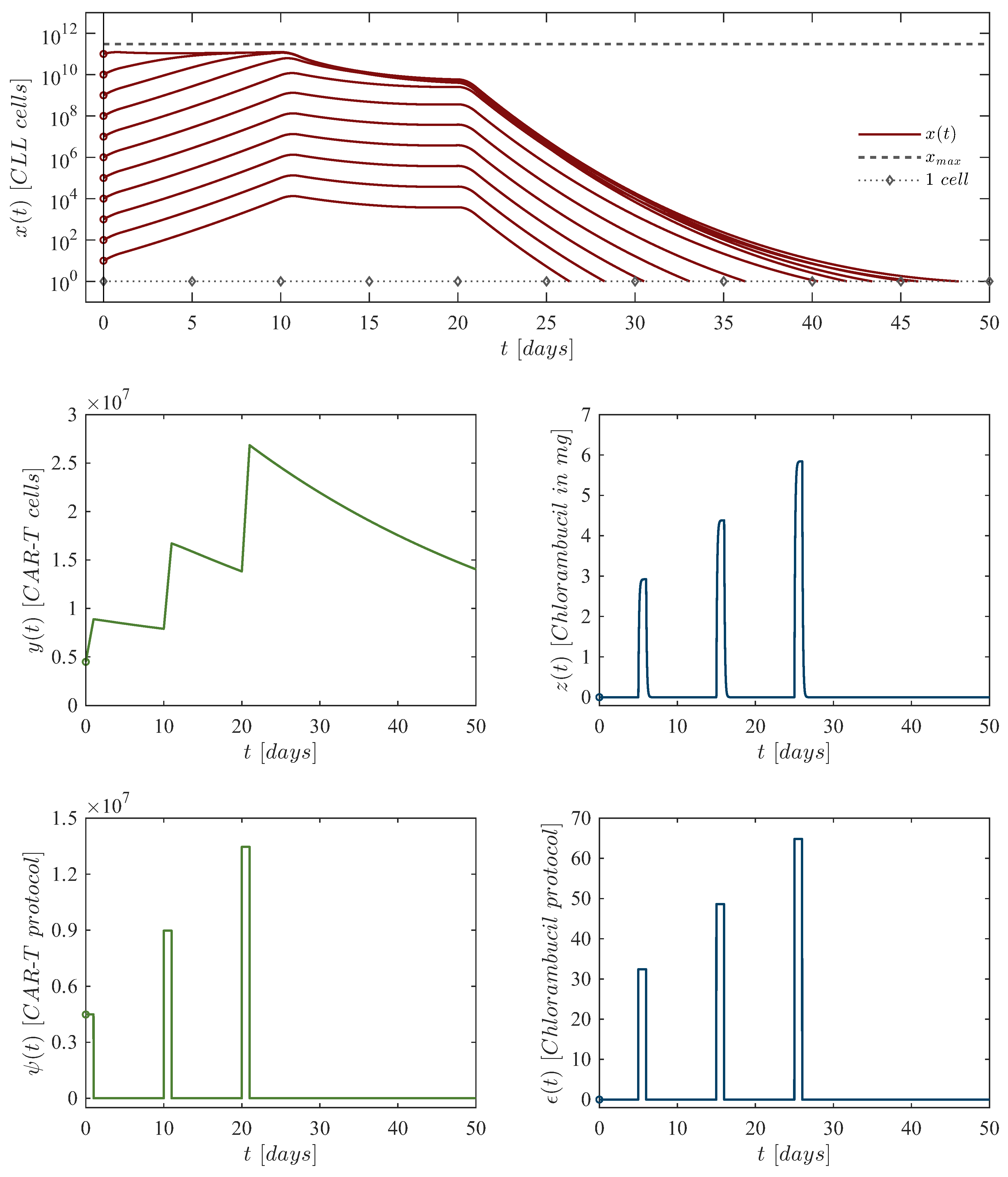
Figure 4.
In silico experimentation for the dose de-escalation chemoimmunotherapy protocol for eleven initial CLL cells concentrations. Dynamics are simulated under the next set of initial conditions: CLL cells with , CAR-T cells, and mg of chlorambucil. Parameter values are as follows: , , , , , , ,
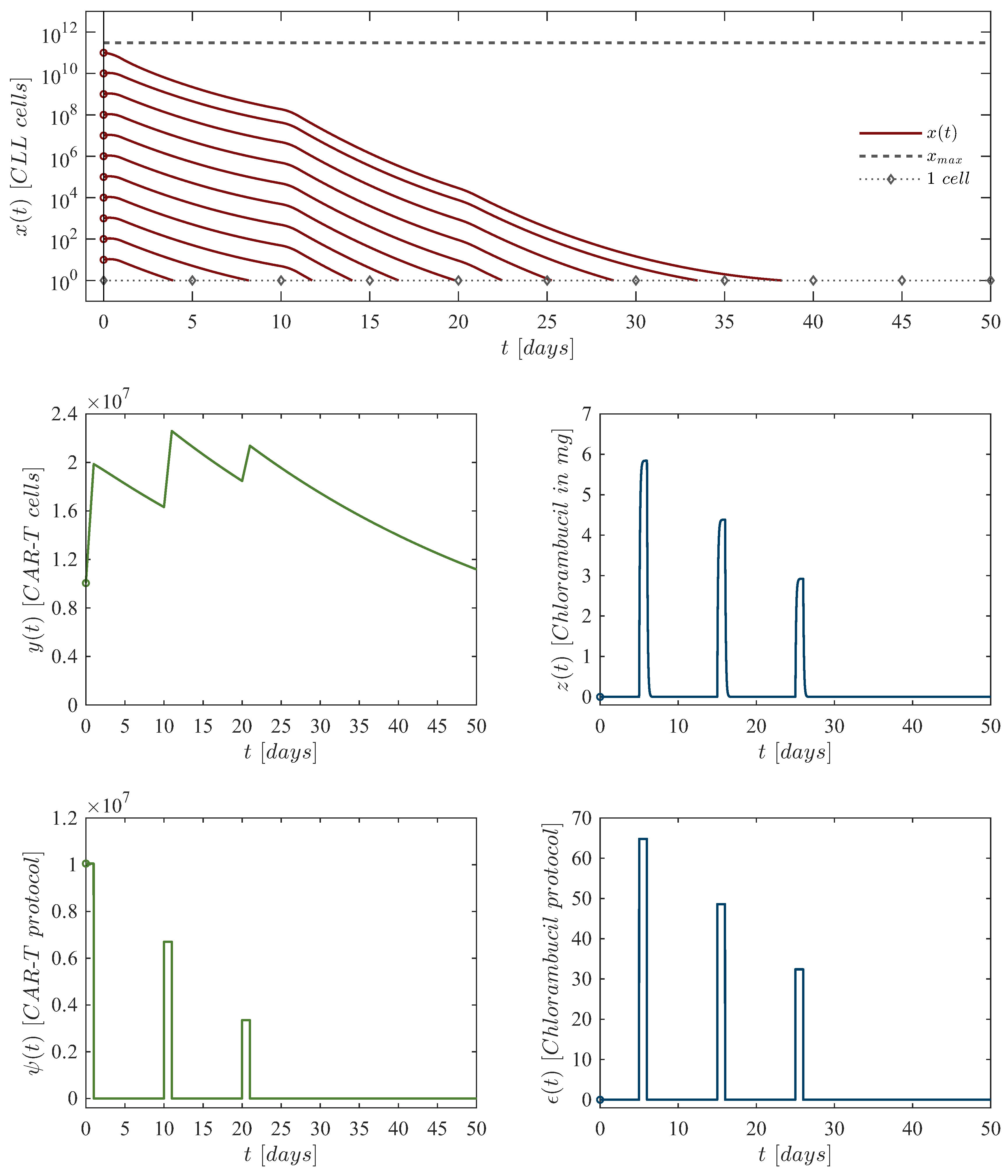
Figure 5.
In silico experimentation performed to illustrate the failure of the dose-escalation protocol. The CAR-T cell doses administered were as follows: cells for the first dose, cells for the second dose, and cells for the third dose. Chlorambucil doses remained consistent with those described in Table 3.
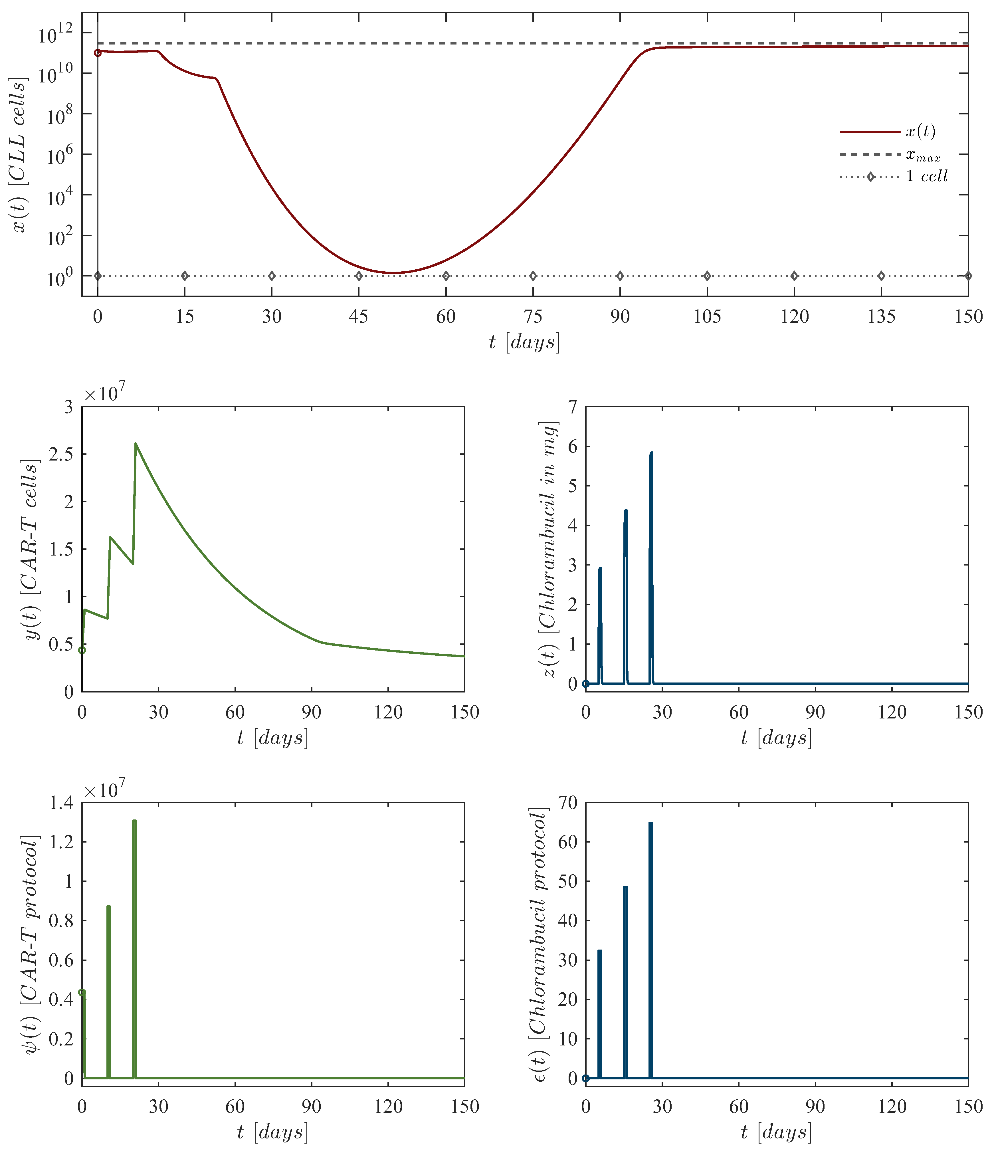
Figure 6.
In silico experimentation performed to illustrate the failure of the dose de-escalation protocol. The CAR-T cell doses administered were as follows: cells for the first dose, cells for the second dose, and cells for the third dose. Chlorambucil doses remained consistent with those described in Table 5.
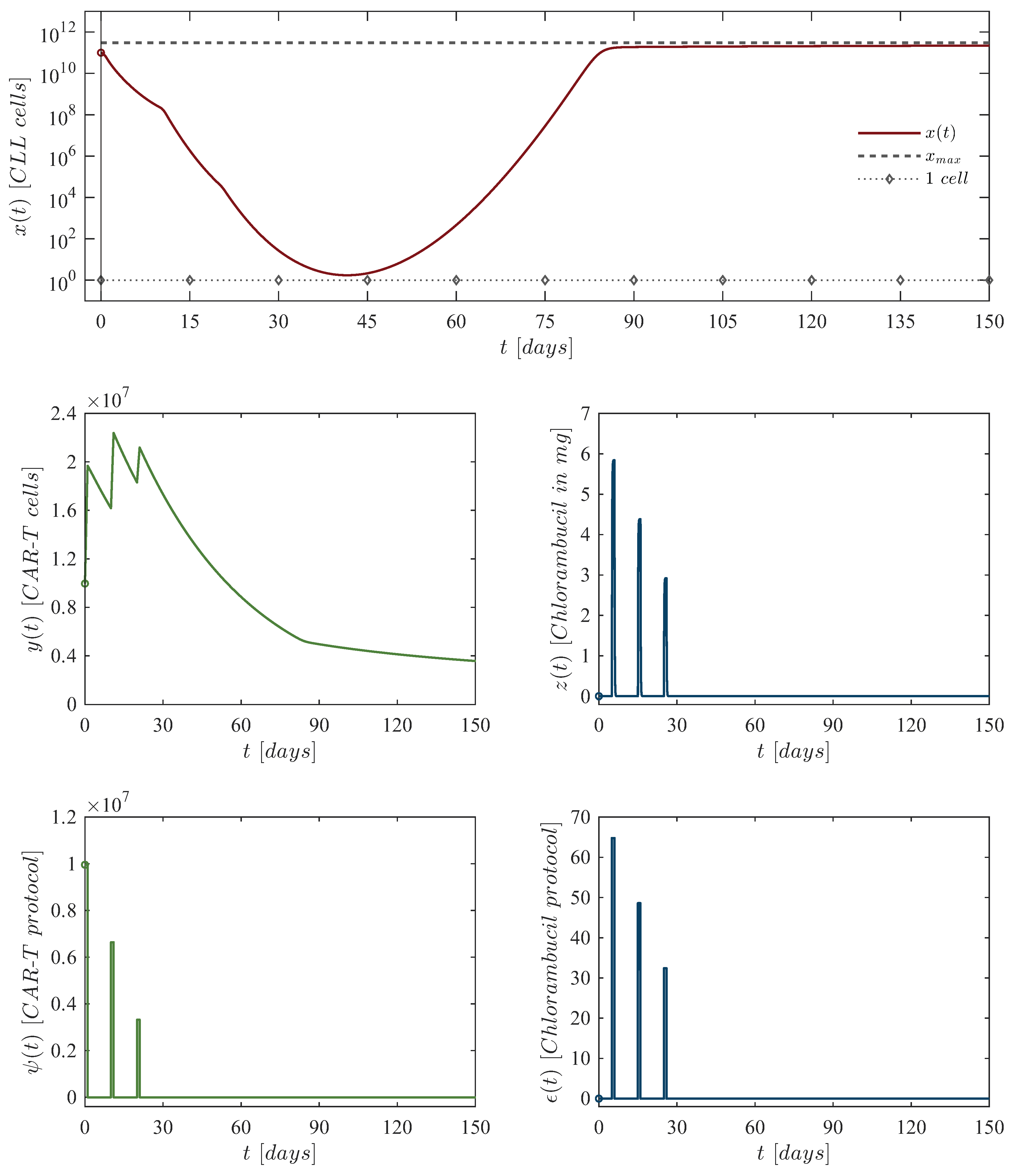

Table 1.
Parameter information for the CLL mathematical model (1)–(3).
Table 1.
Parameter information for the CLL mathematical model (1)–(3).
| Parameter | Description | Units |
|---|---|---|
| CLL cancer cells growth rate | ||
| Maximum leukemia cells carrying capacity | ||
| Eradication rate of CLL cancer cells by CAR-T cells | ||
| Chlorambucil cytotoxicity rate on CLL cancer cells | ||
| Chlorambucil concentration producing of the | ||
| maximum cytotoxicity on CLL cancer cells | ||
| Death rate of CAR-T cells | ||
| Activation rate of CAR-T cells due to encounters | ||
| with CLL cancer cells | ||
| Chlorambucil cytotoxicity rate on CAR-T cells | ||
| Chlorambucil concentration producing of the | ||
| maximum cytotoxicity on CAR-T cells | ||
| Decay rate of the chlorambucil drug | ||
| External CAR-T cell therapy administration | ||
| External chlorambucil drug administration |
Table 2.
Parameter values for the cytotoxicity Equations (5)–(6).
Table 2.
Parameter values for the cytotoxicity Equations (5)–(6).
| Parameter | Value | Units |
|---|---|---|
| Dimensionless | ||
| Dimensionless |
Table 3.
Dose-escalation protocol for the combined application of CAR-T cells and chlorambucil.
| First dose: |
CAR-T cells at day zero, of chlorambucil at day 5. |
| Second dose: |
CAR-T cells at day 10, of chlorambucil at day 15. |
| Third dose: |
CAR-T cells at day 20, of chlorambucil at day 25. |
Table 4.
Chlorambucil cytotoxicity on CLL and CAR-T cells for the selected doses of the drug.
| Chlorambucil dosing | |||
|---|---|---|---|
Table 5.
Dose de-escalation protocol for the combined application of CAR-T cells and chlorambucil.
| First dose: |
CAR-T cells at day zero, of chlorambucil at day 5. |
| Second dose: |
CAR-T cells at day 10, of chlorambucil at day 15. |
| Third dose: |
CAR-T cells at day 20, of chlorambucil at day 25. |
Disclaimer/Publisher’s Note: The statements, opinions and data contained in all publications are solely those of the individual author(s) and contributor(s) and not of MDPI and/or the editor(s). MDPI and/or the editor(s) disclaim responsibility for any injury to people or property resulting from any ideas, methods, instructions or products referred to in the content. |
© 2025 by the authors. Licensee MDPI, Basel, Switzerland. This article is an open access article distributed under the terms and conditions of the Creative Commons Attribution (CC BY) license (http://creativecommons.org/licenses/by/4.0/).
Copyright: This open access article is published under a Creative Commons CC BY 4.0 license, which permit the free download, distribution, and reuse, provided that the author and preprint are cited in any reuse.


