
Submitted:
23 January 2025
Posted:
23 January 2025
Read the latest preprint version here
Abstract
This study adopts the affine term structure three-factor models outlined by , aiming to analyse South African (SA) government bond yields across various maturities. The primary objective is to evaluate whether these models offer robust pricing capabilities—being both admissible and flexible—while capturing the conditional correlations and volatilities of yield factors specific to SA bond yields. For a model to be considered admissible, it must also demonstrate economic identification and maximal flexibility. We thus investigate the short-, medium-, and long-term dynamics of bond yields concurrently. Model estimation involves deriving joint conditional densities through the inversion of the Fourier transform applied to the characteristic function of the state variables. This enables the use of maximum likelihood estimation as an efficient method. We assume that the market prices of risk are proportional to the volatilities of the state variables. The analysis reveals negative correlations between factors. Among the models tested, the A1(3) model outperforms the A2(3) model in terms of fit, both in-sample and out-of-sample.
Keywords:
affine term structure models
; conditional correlation and volatility
; three-factor models
; market price of risk
1. Literature Review
This paper explores the behaviour of the SA interest rates in terms of historical time series and a cross-section of yields across a maturity spectrum. Inspired by the seminal work of [1], we proceed by implementing their model and its maximal counterpart. Among three options of models tested on US Treasury swaps, their was found to perform better than other models, followed by their . However, high time-varying conditional volatility was exhibited at the expense of conditional correlations. Initially, they consider a comprehensive framework for the specification, analysis, and classification of Affine Term Structure Models (ATSMs). They provide a complete characterisation of admissible and identified ATSMs from which it is required that sufficient general conditions exist; see [2], who describe the regular affine process. They also characterise the sufficient general conditions that must be met for a process to be affine; see [3,4] among others.
ATSMs are among popular models in the vast literature on interest rates term structure and bond pricing. Few examples are the early generation consisting of a single-factor Gaussian of [5], and a square-root process by [6], extended by [7] into a multi-factor. The next generation are the correlated mixture affine models of [1,8], among others. The reason for their popularity is the ability to accommodate stochastic volatility, jumps and correlations among factors driving the asset returns; and lead to computationally tractable closed-form prices, and estimation through moment equations; see [4]. Among research problems addressed using ATSMs is the description and treatment of the co-movement of short and long-term bond yields. An affine process Y is defined as one in which a conditional mean and variance are affine functions of Y. The process is further defined and characterised by [2] as regular affine process, a class of time-homogeneous Markov processes. They consider a state space , for integers and , from which the logarithm of a characteristic function of a transitional probability of such process is affine with respect to the initial state . [4] conveniently formalises it in terms of their exponential-affine Fourier (for continuous-time) and Laplace (for discrete-time) transforms. The affine relationship is defined by coefficients which are solved by a family of ordinary differential equations (ODEs). These ODEs are the essence of tractability of regular affine processes. [8] apply the ODEs as time-dependent drivers of the solution to a zero-coupon bond, provided the parameters are admissible. An inverted form of these zero-coupon bond gives rise to a yield as a state variable. They also exploit the idea of a yield-only analysis without including additional economic variables as latent factors.
[9,10] are among several authors who have approached the application of ATSMs in discrete-time although they are known to have less popularity compared to their continuous-time counterparts. Earlier models exhibited a tendency of perfectly correlated returns of bonds of all maturities, which is an unrealistic behaviour and unsuitable for hedging; see [11]. Several authors extended these one-factor Markov representation of a short-rate by introducing a range of multi-factor models with the long-run mean , and the stochastic volatility of that are affine functions of for which [1] explores several specifications. [12] endorse a parsimonious representation of the yield curve matching the time series and cross-sectional variation of bond yields through three-factor models. They develop a simple estimation approach by exploiting the exponential-affine structure of these models; see also [13] on the stochastic mean and stochastic volatility and three-factor model of the term structure of interest rates and its applications in derivatives pricing and risk management
A specification of an ATSM should be "admissible" and therefore lead to well-defined bond prices. The admissibility property is completely characterised by [2] in the "canonical" state space , with a non-negative diagonal matrix. However, this property has a problem of imposing parameter restrictions on the affine process to ensure that it is well defined. One typical scenario is the restriction of parameters to ensure that the conditional variance of a state variable remains non-negative. The requirements for admissibility become more complex as the number of state variables determining conditional variances increase; see [4]. The admissibility condition ensures that the process does not exit the domain . A family of models with a domain are a common admissible family of models; where M factors evolve in a positive state space while evolve in an unrestricted space; see [14]. [1] verifies this easily through admissible factor ATSMs that are uniquely classified into non-nested subfamilies.
Admissible models should also be canonical, meaning that they are economically identified, and maximally flexible; see [4]. As a result, the benchmark ATSM models should have a canonical representation and also satisfy the non-negative and non-explosive solution of ([15]). Their drift should satisfy a Lipschitz condition, and the diffusion should satisfy the uniqueness condition of [16]; see [3]. These conditions have an effect of restricting the correlation structure of the affine diffusions. Exploiting the Gaussian and square-root form of diffusions, there still appear to be non-satisfaction of the regularity conditions of non-explosive growth and uniqueness, giving rise to need for a Feller condition;1 see [3]. A multi-dimensional extension of a Feller condition was implemented by [8], which was found to handle the general correlated affine diffusions. The condition ensures that only positive factors enter the volatility . This involves restrictions on the state variables that prevent the instantaneous conditional variances from becoming negative. This condition is sufficient for the existence of a unique solution to the affine SDE according to [2].
For each of the subfamilies, there exists a maximal model that is econometrically plausible for all other models within this subfamily. They describe further the maximal models in relation to the classification; and highlight an interaction within the family of ATSMs between the dependence of the conditional variance of each on and the admissible structure of the correlation matrix for Y. A key advantage of maximal models is that of overcoming the overidentifying restrictions that are imposed on yield curve dynamics; see [1]. The admissibility property is also confirmed by the no-arbitrage solution for a zero-coupon bond following [8].
[1] specification applied the continuous-time approach to the ATSMs which is popular to a majority of empirical literature. They explore the structural differences and relative goodness-of-fits of ATSMs. They refer to a trade-off between flexibility in modeling the conditional correlations and volatilities of the risk factors. They classify a family of factor affine into non-nested subfamilies of models. From their three-factor ATSMs, empirical analysis suggests that some subfamilies of ATSMs are better suited than others to explaining historical interest rate behaviour.
The focus of the research is to implement the specifications of [1] to test the pricing of zero-coupon bonds and forecasting the yield curve dynamics when using the SA bond yield. It also attempts to extract the latent factors from the yield itself, without any consideration for other economic factors; see [8]. ATSMs are proven to dominate both theoretical and empirical frameworks in term structure modelling; see [3]. A link between the cross-sectional and time series properties is made consistent by the ATSMs. Evolution of unobserved factors from the risk-neutral dynamics of the yield are proved to have both the drift and the diffusion coefficients as affine functions of such factors by the ATSMs; see [3]. Several methods of estimation are available and require mostly the knowledge of the joint conditional density of yields. In this study, we follow the estimation method of Fourier inversion for the characteristic function of a state variable, which is assumed to lead to a conditional density. This method leads to a closed-form solution where the maximum likelihood is an efficient estimator.
2. Model Establishment
We discuss the model in the context of admissibility of ATSMs. In the absence of arbitrage opportunities, a zero-coupon bond that matures at time T is priced as
where:
is the price of a bond at time t maturing at time .
t is the current or initial time at which the bond is evaluated.
is the maturity date, at which the bond pays its face value.
s is a continuous time variable at which the interest rate process evolves.2
denotes the conditional expectation under the risk-neutral measure Q given the information available at time t.
To obtain an factor ATSMs it is assumed that an instantaneous short-rate is an affine function of a vector of N unobservable state variables , written as
where and .
Another assumption is that follows an affine diffusion
and represent the reversion rate and central tendency (long-term mean) parameters under risk-neutral measure, respectively. is an dimensional independent Brownian motion under the risk-neutral measure Q; , and are matrices, which may be asymmetric or non-diagonal. is a diagonal matrix with the diagonal elements written as
where and .
[8] has the following time dependent solution to the price of a zero-coupon bond, provided that parameters are admissible.
and the related yield is computed as
where and are coefficients whose solution satisfies the following ODEs (Ricatti equations)
A solution to these ODEs is found through numerical integration, starting from the initial conditions =. Risk-neutral dynamics of the short rate in (2) through to (4) determine this specification of the ODEs.
To use the closed-form representation of (1) in the empirical study of ATSMs, it is required that the distributions of and under actual physical measure P be known. To this end, a market price of risk is introduced as
where is an vector of constants. The process under physical measure P, therefore also has an affine form 3
Note that a superscript Q has been removed. is an dimensional vector of independent Brownian motion under P, , . comprises of in its row, and is an vector with as its element.
3. A Canonical Representation of ATSMs
According to [1], a general specification for (10) may not always lead to a positive conditional variances over a range of Y, given an arbitrary set of parameters . However, admissibility requires that parameters restrict in (10) to be strictly positive for all i; where denotes the matrix of coefficients on Y in .
From (4), there is a special case where there is no admissibility problem when , for all i, since the instantaneous conditional variances are all constant. Outside the special case, it is necessary to impose constraints on the drift parameters and , and diffusion coefficients and . The requirements for admissibility become more restrictive as a number of state variables determining increases.
They consider a case where there are M state variables driving the instantaneous conditional variance of the vector Y, such that . They further propose a set of benchmark models as the most flexible econometrically identified affine DTSM on the state space ; see also([2]). It is only when the admissibility conditions are met that a canonical representation may be defined.
Definition 3.1: For each M, is partitioned as where is , and is ; where V and D represent the volatility sources and the dependent factor, respectively. The canonical representation of the benchmark model is defined as a special case of (3) with
for , and is either lower or upper triangular for .
The canonical representation of is the mean-reversion matrix, with diagonal terms expected to pull the mean level to non-negativity, thus influencing positive variances. Its off-diagonal terms on the other hand reflect how different state variables influence each other, indicating potential dependencies or interactions that could affect the overall system behaviour. The matrix therefore captures both the stabilising effects of the mean-reversion rates and the dynamic interplay between different state variables. In the three-factor analysis, this trade-off between non-negative variance and correlations requires a special attention. It also has an impact on the choice of M, number of state variables entering volatility and the interactions among factors
The following parameter restrictions are imposed:
[1] define a subfamily ; of affine DTSM as nested special cases of the canonical model or its invariant transformation; where . Equivalent affine models are obtained under invariant transformations that preserve admissibility and identification and leave the observable quantities like short rate unchanged. Details on invariant transformation are discussed in Appendix A of [1].
The following issues are further noted from [1]:
The assumed structure of ensures that for the canonical representation. To verify that M resides in , instantaneous conditional correlations among are zero, whereas the instantaneous correlations among are determined by parameters because . Admissibility is established provided (20) holds, and that the conditional covariance matrix of Y depends only on . Zero restrictions in the upper right block of and the constraints in (18) and (19) ensure that is positive. Stationarity is also assured by ensuring that all the eigenvalues of are strictly positive; see also Appendix B in [1].
In addition to an admissible canonical representation, in which the minimal known sufficient condition for admissibility were imposed, minimal normalisations for econometric identification are imposed to derive a "maximal" model in . A more unique class of maximal , referred to as the equivalence class of model is obtained by invariant transformation of the canonical representation; see Appendix A in [1].
[1] further points that the canonical representation of models may not always be a practical way for analysing state variables in ATSMs. Often, existing literature opted for parameterising ATSMs with the riskless rate r as a state variable, resulting in "affine in r" (Ar) representation. This can be rewritten as an "affine in Y" , where can be expressed as an unobserved state vector . As a result, a thorough specification analysis for factor ATSMs necessitates evaluating non-nested, maximal models, and ensuring that a thorough understanding of the model’s structure and implications is obtained.
4. The Three-Factor Affine Term Structure Models
Three-factor models are used to describe the historical behaviour of the term structure of interest rates. Traditionally, these factors are unobserved (latent) and can only be defined statistically using techniques such as principal component analysis to convey economic meaning. Popular yield-curve fitting approaches such as the dynamic Nelson-Siegel model apply PCA loadings to fit a yield curve; see [19]. These approaches appear to fit and forecast well but lack the theoretical rigour to enforce some no-arbitrage restrictions. Contrary to the yield-curve fitting approaches, the empirical approaches to the factor models such as the ATSMs are worth pursuing. They consider the maximal parameterisation through which in general the economic identification of factors can be revealed. The paper by [12] is among early works that are based on enforcing the no-arbitrage restrictions by implementing the three-factors models. They constructed a simple affine model with short term interest rate, mean rate and volatility as three factors, which are easy to estimate. They further conclude that the short rate plays and important role in yield curve modeling, following their observation that it could not be dominated by any other factor across all maturities.
[1] explores various forms of the canonical ATSMs and their maximal counterparts, as influenced by the number conditional volatility and correlation of factors. Fixing these factors into gives rise to their three-factor models which posit mainly the representation of the short-rate itself, its mean rate and volatility as the three-factors. Analysis and comparisons are made of the Gaussian versus the square root diffusion forms of the models, even though the latter appear to be preferred as it imposes the non-negative variance restrictions.
Three-factor models were derived from the notation where M is the number of state variables that enter volatility according to [1]. Emphasis has been put on the trade-off between conditional volatility and correlation as a focus for the analysis of the term structure of interest rates. As previously discussed, [8] introduced a multi-dimensional Feller condition. It ensures that negative state factors do not enter the volatility by restricting correlations; see also [3]. We have previously also discussed in a similar context, the role of the mean-reversion rate matrix , its non-negative diagonal terms restrictions and interactions among state variables through its off-diagonal terms.
A number M of the factors that drive the process which enters a volatility become the main argument on the choice of an model, depending on the purpose of the study. [20] point out that more volatility factors result in less flexibility in allowing risk premium and correlation structure. As a result, they are in favour of a one conditional volatility factor models such as the by [1]. [21] also favour the with and for the same purpose of allowing flexibility for risk premium and correlation. Their focus is to impose restrictions on the parameters of such that the volatility factor disappears from the bond pricing equation. In our approach, we analyse the admissibility of parameters and cross-equation restrictions that result from interactions among the factors . As previously discussed, the mean-reversion rate matrix has elements with either negative of positive magnitudes playing a role of ensuring that factors are pulled from entering the variance only for non-negative values, otherwise non-negative correlations are the result. This is also applicable in the case of a three-factor model.
In this study we focus on the , models and their maximal counterparts and to determine both the fit and estimation when applied to the SA bond yield curve.
4.1.
These models are characterised by one factor Y as a source of conditional volatility. As a result, gives rise to the model form of . From the original [12] BDFS model, the according to the notation of [1] is specified as
where:
The state variables , and are the stochastic volatility for , central tendency or long-run mean of and short rate processes, respectively. The volatility affects the short rate through its volatility factor . The coefficient represents the rate at which the short rate reverts to the central tendency. The stochastic volatility also enters and it is also instantaneously correlated with as noted in the last term .
The maximal model is best suited for interpreting the parameter restrictions. As a result, [1] prefer the following model in (23) as a maximal which is affine in r. They determine their by relaxing the parameters and in order to accommodate a non-zero correlation between the short rate and central tendency. All the other parameters inside the square boxes are set to zero to impose significant restrictions on the dynamics of interest rates and their volatility.
where:
serves as stochastic volatility for , but also enters the drift of , and correlated to as noted in the term ; is the central tendency of r and is the rate at which the short rate reverts to its central tendency. Appendix E in [1] describes the transformation framework from which a test for admissibility and canonical representations in can be achieved.
4.2.
These models are characterised by two factors of Y as a source of conditional volatility. As a result, gives rise to the model form of . The [13] model is the member of this sub-class of models, and it is represented as
, and are independent Brownian motions. The follows a square-root diffusion unlike in the case of the BDFS model. Other parameters , and are the same as in the above models. These leads us to the convenient maximal model for which is represented as
[1] relaxes the restrictions on , and , while other parameters within a square box are restricted to zero.
5. Estimation for Affine Models
The conditional likelihood function is not always known for affine diffusion models. However, a closed-form solution to the ATSMs provides formidable grounds to base the estimation on the conditional characteristic function of a state variable even when the functional form of the density is not known. [22] applied the Fourier inversion to estimate the conditional-likelihood function for a state variable, which leads to an asymptotically efficient estimator of parameters. He also shows that a method-of-moments estimator works well to approximate the efficiency of maximum likelihood of ATSMs from the conditional characteristic function; see also [23].
The conditional density function f of is known up to an inverse Fourier transform of
The charaterisic function for given
From the Proposition 1 of [24], it can be shown that under suitable regulations (5) is the conditional characteristic function of , with and derived from the solution of (7) and (8) for . Therefore, the conditional characteristic function becomes
The log-likelihood form for (27) becomes
By conjecturing the parameters and computing the Fourier inversion, maximum likelihood can be obtained by maximising (30), to obtain a maximum likelihood estimator by characteristic function (ML-CCF); see [4].
[4] considers densities of individual columns , for . A selector vector is assigned an entry 1 and zero elsewhere. The density f of given the entire is the inverse Fourier transform of
Estimation of (31) is based on one-dimensional N integrations instead of dimensional integrations.
The general method of moments (GMM) using a characteristic function is achieved by the residual
For an arbitary instrument ; the estimator becomes
The GMM approach is a beter alternative to a multi-dimensional Fourier inversion. However, as a grid of becomes finer, correlations among moments become increasingly large, leading to a singular distance matrix; see [4].
6. Data Collection
Weekly SA government yields from Thomson Reuters for all the active treasury bonds over the periods October 2013 to September 2024 with maturities 3 months, 5, 10, 12, 20, 25, and 30 years were used. Our in-sample and out-sample data were based on the periods October 2013 - Sep 2023 and October 2023 - September 2023, respectively. The out-sample will be best-suited for forecasting and validation. A summary of descriptive statistics for yields across maturities is presented in Table 1. Mean values range between 6.6% to 10.3% exhibiting an upward slope which is also convex in shape. Recent study by [25] reported a similar behaviour for the average yields. The highest weekly standard deviation of 1.3% is observed for the 3-months maturity which is typical in the short end of the yield curve, suggesting that yields may react quickly to changes in monetary policy or market sentiment. It is followed by a drop to 0.7% and 0.6% for the 5-year and 10-year maturities, respectively. The 20-year maturity exhibits a rise in weekly standard deviation to 1.1%, which may be due to some unexpected economic event. This is also confirmed by a very high kurtosis and negative skewness of 30.69 and -3.23, respectively. After the 20-year maturity, a drop in the weekly standard deviations of 0.9% is observed. This suggests lower volatility and relative stability for the long end of the yield curve.
Table 2 presents the correlations across maturities of yields. The short end of the yield curve is characterised by weak correlations. The 3-month and 5-year terms exhibit negative correlations with their long end counterparts. This may suggest a difference and diversity in dynamics between the short and long end of the yield curve. From the 10-year maturity, higher correlations ranging from 0.608 to 0.999 are observed, suggesting stability as the yield curve approaches its long end.
Figure 1 presents the first three principal components (PC) of the yields over maturities. They are explained by the variance of about 96.32%, which is close to the 98% empirical finding according to [26]; see also [3,19]. The first PC represents a key rate shift or level change in rates. It is the result of volatility causing rates of all maturities to fluctuate by almost the same amount. The observation is that short end is associated with high volatility and increasing rates. At mid-term around the 10-year maturity they reach a peak, followed by stability as they approach the long end of the yield curve. The second PC represents a slope which exhibits a hump in the short end associated with rate increase, followed by a drop in rates in mid-term region and stable but falling rates towards the long end. Volatility forces a fall in rates in the short end followed by a slight increase up to mid-term, 10-year maturity, thereafter, increases until it falls and stabilises towards the long end.
The behaviour of PCs is also associated with the correlations as discussed earlier, where short end is associated with weak correlations whereas in the long end of the yield curve, strong correlations were observed. These patterns are suitable for trading in swaps and correlation-based hedging strategies. Our focus being the ATSMs, we believe that these PCs are somehow closely related to the latent factors derived by the solution of coefficients and in (6). The three-factor models with three labels short-rate, volatility and central tendency should exhibit nearly a similar pattern to PCs; see [3].
Figure 2 presents a selection of observed yields from the SA Treasury bonds plotted against maturities of up to 30 years. A spread between 5 and 20 years is also plotted and expected to represent a slope. Crossovers are observed among individual plots from time to time, indicative of either positive or negative (inverted) yield curves. Initial unobserved inputs to the three-factor simulation of are selected from a 3-month yield, a spread between 5-year and 20-year yields, and a 30-year yield. We apply these rates together with the initially guessed parameters to simulate the state variables from (10). These are further used as inputs to the solution of ODE (7) and (8) from which coefficients and are obtained. Thereafter, a model-based set of zero-coupon bonds and zero-yields are obtained from (6). The selection is also guided by the observations from the PCA, suggesting that our selection is a proxy for level, slope and curvature, taking into consideration the PCA features for short end, mid-term and long end.
7. Scenario Determination
Our objective is to fit the ATSMs using the SA bond yield curve to extract the latent factors by way of zero-yields. From these zero-yields, we pursue a three-factor approach to model specifications in the following scenarios.
- Evaluate the performance of model and its maximal counterpart from in-sample. Ensure that parameters are admissible and that models meet the canonical form in-sample
- Evaluate the performance of model and its maximal counterpart from in-sample. Ensure that parameters are admissible and that models meet the canonical form in-sample
- Estimate both models and their counterparts out-sample and evaluate their performance.
Further, we draw more insight from optimisation results and statistical analysis. In all the scenarios, we assume the market price of risk is completely affine and of the form .
8. Model Implementation
8.1. Three-Factor Models
The first three principal components are selected as proxies to the required three factors. Their initial values are inputs to both the and and their maximal counterparts. The observed market yields are therefore selected from 3-month, spread between 5-year and 20-year, and 30-year yields. The observed yields are used to calibrate parameters, which are then applied to estimate the models. Solution to SDE is initialised by the initial state vector and parameters to obtain , and . The market price of risk associated with each of these factors are also computed by derived equations, following a transformation process; see Appendix E in [1].
The three-factors models are further calibrated using the ML-CCF which is an efficient estimator for the log-likelihood function. The calibration process identifies optimal parameters and the maximum of the log-likelihood function. In addition, the scores of likelihood functions are used to identify the market price of risk parameters; see [22,27]. The same assumptions of completely affine price of risk are made regarding market price of risk. Individual parameters , and are assumed to be easy to identify in the case where time-varying volatility exists. The scores of likelihood function are also applicable to identify the market price of risk as the parameters , and are expected to be non-constant nor collinear. From the invariant transformations, [1] derives the equations to compute these parameters in Appendix E.
9. Analysis of Results
9.1. In-Sample Analysis
9.1.1. and Models
In-sample data were applied to implement both models through SDE’s, from which variables , and for stochastic volatility, central tendency and short rate, respectively were produced. Market price of risk parameters , and , are also obtained from the results of these SDE according to the formulation from Appendix E in [1]. A linear combination of these variables result in a short rate that is fitted according to the affine function (22). The process is followed by implementation of optimisation techniques from which an efficient maximum likelihood and parameters estimates are obtained.
Table 3 presents the estimation results for both model and its maximal counterpart . Estimation results are based on the Fourier inversion of the characteristic function ML-CCF of the factor from (30). Variables , and were simulated from (23) where initial guess parameters, and the initial vector of factors for , at time t, were inputs. According to [1] the BDFS model is a special case of (23) with the parameters in square brackets restricted to zero. However, in their specification, parameters and are relaxed and can be assumed take any other non-zero value.
The Nelder-Mead algorithm was used as it does not require a computation of gradients or second derivatives. This is despite its significant limitation that it cannot directly produce standard errors for the parameter estimates due to its inability to compute the Hessian matrix. To evaluate model goodness-of-fit and performance, we relied on the Chi-square () statistics. Both AIC and BIC indicate how model complexity was penalised, taking into account both fit and the number of parameters.
AIC and BIC are both lower for compared to indicating to be slightly better at balancing model complexity while it also has slightly more parameters. However, differences between AIC and BIC values, such as -866.21 vs.-866.33 for AIC, and -769.36 vs. -769.48 for BIC are quite small, suggesting that the models might be very similar in performance. Nonetheless, seems to be marginally better. The model with a lower of 57.16, which is the appears to have a better fit than the with a of 87.57.
Parameters , , and are restricted to zero for the model, whereas they are relaxed for the maximal model . In addition, some negative correlations were introduced for and . A small movement in after calibration from zero to 0.035 for is exhibited. This suggest that the model has incorporated a weak positive relationship between short rate and volatility, which could reflect realistic market dynamics, though the effect is not large enough to dominate the model’s outcomes.
For model there is no change in from -0.094 to -0.094 after calibration which is interpreted as an almost unchanged relationship between the volatility of the central tendency and short rate r. For a change to 0.089 reflects a slightly weak inverse relationship between the volatility of and r. is therefore slightly less sensitive to the impact of central tendency volatility on short rate volatility.
In the case of , has calibrated from-3.420 to -3.509 suggesting a modest increase in the negative relationship between the volatility of the short rate r and and the central tendency . This implies a slightly more negative correlation between the central tendency volatility and the volatility of the short rate. For a change from -3.420 to -3.786 indicates a significant increase in the negative correlation between the volatility of r and . In summary, exhibits a weaker relationship with volatilities while in the case of a slightly stronger negative correlation between short rate and central tendency is observed.
Further analysis was performed to test the residuals resulting from model-implied factors from both and versus market observed yields. It is expected that the residuals are characterised by a normal distribution. Figure 3 presents qq-plots in respect of residuals for the three factors. Despite some skewness and variations as exhibited by a red line, there seem to be less significant deviation from symmetry as can be seen from slight diversions of the red from the blue line. Therefore, all the subplots suggest a normal distribution for residuals. Based on the test, a p-value of 1 for both models also confirm that the residuals perfectly match the expected distribution. However, there are some concerns that a p-value of 1 is unusual and unlikely and could suggest overfitting.
9.1.2. and Models
Table 4 presents the results of parameter estimation for both models and . The second column list the initial guesses of parameters4. The third and fourth columns report the estimates of parameters that result from the optimisation.
Nelder-mead algorithm converged after 1574 and 1471 for models and , respectively. Both AIC and BIC are almost the same, suggesting that either one of them is worth a selection from a model complexity perspective. However, individual differences of -3455.43 vs -4483.99 for AIC, and -3350.51 vs -4379.07 for BIC, model to be slightly better at balancing model complexity while it also has slightly lower parameters. statistics of 77.26 and 96.01 for models and , confirm to be a good fit. The same applies to the p-values of 1 for each model, which may suggest a good fit, except for the issue of possible overfitting.
Parameter under model moves from -33.900 to -33.989 suggests a stronger mean reversion which may lead to lower stochastic volatility and a more stable behaviour of the short rate. For model it moves to -12.427, indicative of weaker mean reversion, higher stochastic volatility and more variability in the short rate. For , exhibit a small movement from -35.300 to -35.393 (a difference of 0.0931). This suggest a relatively stable relationship between short rate and volatility, and a slight increase in volatility. A large negative value in for is observed, meaning that even a small change in the short rate would have a large effect on volatility.
The covariance parameters in exhibits a move from -182.000 to -182.420 which is a modest increase in the negative relationship between the short rate r and volatility . This implies a slight increase in negative correlation between the r and . For a change from -182.000 to -133.403 indicates a significant increase in the negative correlation between the r and . It is apparent that exhibits a slight increase in relationship with volatilities while in the case of a slight increase in negative correlation between r and is observed.
A plot for residuals suggests a not so poor a model fit despite a slight deviation from normality due to a slight skewness and asymmetry. Figure 4 presents a qq-plots for residuals based on the observed yields and the first three factors. Variation and skewness suggest a slight deviation from normality even though acceptable in terms of the stylised facts for assets and returns.
9.2. Instanteneous Short Rate
Table 5 presents the average weekly short rate, standard deviation and annualised volatility for model-implied instantaneous rates that were computed from (22) and (25). The rates were computed for subfamilies , and their"maximal counterparts. They are compared to the related statistics for a three-month yields (a proxy for short rate), as reported in Table 1. Model exhibits an average short rate value of 5.1% which is closer to the weekly mean value of 6.6% for the observed three-month yields. The model exhibits highest weekly standard deviation and annualised volatility of 2.8% and 20.3%, respectively. This is followed by 1.9% and 13.9% weekly standard deviation and annualised volatility, respectively, exhibited by the maximal model . The and suggest higher volatility than the and subfamilies.
Figure 5 plots the model-implied instantaneous rate against maturities. Both and in blue and magenta, respectively. The plots are based on estimated parameters fitted to the models. and its maximal counterpart are plotted against maturities in Figure 6.
The model-implied instantaneous short rate functions from (22) and (25) are made up of a linear combination of factors mapped to , and and representing volatility, central tendency and short rate, respectively. They exhibit an average 11.9% and 8.1% short rates for and , respectively. The and models exhibits higher volatility than the and models. As the instantaneous rate evolves, mean-reversion persists throughout the process. Both subfamilies of models suggest that a positive but stable economic growth is forecasted, exept for a higher volatility as reflected in and plot.
9.3. Out-Sample Analysis
Table 6 presents a comparison of the out-sample performance for both models and and their maximal counterparts. Model appears to be have a good fit according to the statistic of 8.26 versus 9.20 of the .These are also considered relative to their respective degrees of freedom. Vast differences between the out-sample figures when compared to in-sample might be due to the size of data series. However, the out-sample perfomance of the models fit well. Morover, the p-values exhibit a promising improvement which suggest a better fit for the models.
10. Conclusion
The historical behaviour of the term structure of interest rates for the SA treasury bond was analysed. The purpose was to establish whether the ATSMs specifications of the three-factor models were suitable for the data. The study also considered the conditional volatilities and correlations of the state variables as they are essential components. It has therefore been essential to thoroughly examine the interactions among the state variables—stochastic volatility, central tendency, and the short rate—within the framework of a three-factor approach to the ATSM.
Model is a suitable specification for the data, even though it suggests a weaker relationship between the short rate and its stochastic volatility. Based on the Chi-square test, the model out-performs its maximal counterpart . exhibits a stronger negative correlation between short rate volatility and central tendency volatility. Similar circumstances prevail for the model and its counterpart, although negative correlation tends to strengthen more from modest level with to even stronger with
As an initial guess to the parameters, we adapted the empirical estimates in [1]. This includes both their assumptions in regard to both parameters that were fixed to (zero) and those allowed to be unrestricted. The reason behind unrestricted parameters is to enable flexibility of interactions between conditional volatility and correlations. Resulting post-calibration estimates suggest a good fit for our data.
There were some limitations to the approach, which should be considered for future research. First, the inability to perform a detailed analysis on the market price of risk impact to the specifications. Second, the models were based only on the diffusion process and do not explicitly incorporate the impact of jumps.
Author Contributions
Conceptualization, M.M. and G.V.; methodology, G.V.; software, M.M; validation, M.M, and G.V.; formal analysis,M.M., and G.V; investigation, M.M and G.V.; resources, M.M and G.V; data curation, M.M and G.V; writing—original draft preparation, M.M; writing—review and editing, G.V.; visualization, M.M.; supervision, G.V.; project administration, G.V.; funding acquisition, None. All authors have read and agreed to the published version of the manuscript.
Funding
This research received no external funding.
Institutional Review Board Statement
Not applicable.
Informed Consent Statement
Not applicable.
Data Availability Statement
The data that support the findings of this study are available from the authors upon reasonable request.
Acknowledgments
None.
Conflicts of Interest
None.
Abbreviations
The following abbreviations are used in this manuscript:
| ATSM | Affine term structure models |
| AIC | Akaike information criterion |
| BIC | Bayesian information criterion |
| BDFS | Balduzzi P, Das SR, Foresi S |
| DTSM | Dynamic term structure models |
| GMM | Generalised method of moments |
| ML-CCF | Maximum likelihood estimator by conditional characteristic function |
| ODE | Ordinary differential equation |
| PCA | Principal component analysis |
| SDE | Stochastic differential equation |
References
- Dai, Q.; Singleton, K.J. Specification analysis of affine term structure models. The journal of finance 2000, 55, 1943–1978. [Google Scholar] [CrossRef]
- Duffie, D.; Filipović, D.; Schachermayer, W. Affine processes and applications in finance. The Annals of Applied Probability 2003, 13, 984–1053. [Google Scholar] [CrossRef]
- Piazzesi, M. Affine term structure models. In Handbook of financial econometrics: Tools and Techniques; Elsevier, 2010; pp. 691–766. [Google Scholar]
- Singleton, K.J. Empirical dynamic asset pricing: model specification and econometric assessment; Princeton University Press, 2006. [Google Scholar]
- Vasicek, O. An equilibrium characterization of the term structure. Journal of financial economics 1977, 5, 177–188. [Google Scholar] [CrossRef]
- Cox, J.C.; Ingersoll, J.E.; Ross, S.A. An analysis of variable rate loan contracts. The Journal of Finance 1980, 35, 389–403. [Google Scholar] [CrossRef]
- Langetieg, T.C. A multivariate model of the term structure. The Journal of Finance 1980, 35, 71–97. [Google Scholar]
- Duffie, D.; Kan, R. A yield-factor model of interest rates. Mathematical finance 1996, 6, 379–406. [Google Scholar] [CrossRef]
- Dai, Q.; Le, A.; Singleton, K.J. Discrete-time dynamic term structure models with generalized market prices of risk. 2006. [Google Scholar]
- Darolles, S.; Gourieroux, C.; Jasiak, J. Compound autoregressive processes. Unpublished working paper. CREST 2001. [Google Scholar]
- Aït-Sahalia, Y.; Kimmel, R.L. The Econometrics of Fixed-Income Markets. In Handbook of Fixed-Income Securities; 2016; pp. 265–281. [Google Scholar]
- Balduzzi, P.; Das, S.R.; Foresi, S. A simple approach three-factor affine term structure models. 1996. [Google Scholar]
- Chen, L. Stochastic mean and stochastic volatility: a three-factor model of the term structure of interest rates and its applications in derivatives pricing and risk management; Blackwell publishers, 1996. [Google Scholar]
- Tebaldi, C.; Veronesi, P. Risk-Neutral Pricing: Monte Carlo Simulations. In Handbook of Fixed-Income Securities; 2016; pp. 435–468. [Google Scholar]
- Ikeda, N.; Watanabe, S. Stochastic differential equations and diffusion processes; Elsevier, 2014. [Google Scholar]
- Yamada, T.; Watanabe, S. On the uniqueness of solutions of stochastic differential equations. Journal of Mathematics of Kyoto University 1971, 11, 155–167. [Google Scholar] [CrossRef]
- Hirsa, A. Computational methods in finance; CRC Press: Boca Raton, FL, 2013; pp. 11–22. [Google Scholar]
- Rouah, F.D. The Heston model and its extensions in Matlab and C; John Wiley & Sons, 2013. [Google Scholar]
- Diebold, F.X.; Piazzesi, M.; Rudebusch, G.D. Modeling bond yields in finance and macroeconomics. American Economic Review 2005, 95, 415–420. [Google Scholar] [CrossRef]
- Andersen, T.G.; Benzoni, L. Can bonds hedge volatility risk in the US treasury market? A specification test for affine term structure models; Technical report, Working paper; Kellogg School of Management, Northwestern University, 2005. [Google Scholar]
- Bikbov, R.; Chernov, M. Term structure and volatility: Lessons from the Eurodollar markets. Available at SSRN 562454 2004. [Google Scholar] [CrossRef]
- Singleton, K.J. Estimation of affine asset pricing models using the empirical characteristic function. Journal of Econometrics 2001, 102, 111–141. [Google Scholar] [CrossRef]
- Carrasco, M.; Chernov, M.; Ghysels, E.; Florens, J.P. Efficient estimation of jump diffusions and general dynamic models with a continuum of moment conditions. Available at SSRN 338961 2002. [Google Scholar] [CrossRef]
- Duffie, D.; Pan, J.; Singleton, K. Transform analysis and asset pricing for affine jump-diffusions. Econometrica 2000, 68, 1343–1376. [Google Scholar] [CrossRef]
- Shu, H.C.; Chang, J.H.; Lo, T.Y. Forecasting the term structure of South African government bond yields. Emerging Markets Finance and Trade 2018, 54, 41–53. [Google Scholar] [CrossRef]
- Litterman, R.B.; Scheinkman, J.; Weiss, L. Volatility and the yield curve. The Journal of Fixed Income 1991, 1, 49–53. [Google Scholar] [CrossRef]
- Carrasco, M.; Chernov, M.; Florens, J.P.; Ghysels, E. Efficient estimation of jump diffusions and general dynamic models with a continuum of moment conditions. 2000. [Google Scholar]
| 1 | A condition is met when ; where represents the mean reversion speed, and the mean reversion rate. It ensures that the drift is sufficiently large to guarantee a positive variance. |
| 2 | The state variable Y is a Markov process, therefore the future state at time s depends only on the current state at time t and not on the history before time t. Y satisfies the Markov property; see definition 5.1 in [4]. |
| 3 | Continuous-time SDE are better treated in discrete form using methods such as the Euler approach. A discretised version also ensures a positive truncation for the variance; We approximate as ; where is the approximation of at time ; is a standard normal variable. Several authors discuss these discretisation schemes; see [17] : page 229 and [18] : page 177. |
| 4 | The parameters we used as initial guesses are based on the estimates according to [1]. We find these parameters to be the best starting point as they have empirically been tested to result in convergence. The same approach was also applied in the case of our and models |
Figure 1.
Loadings of the first three principal components of the yields over maturities. Data were retrieved from Thomson Reuters.
Figure 1.
Loadings of the first three principal components of the yields over maturities. Data were retrieved from Thomson Reuters.
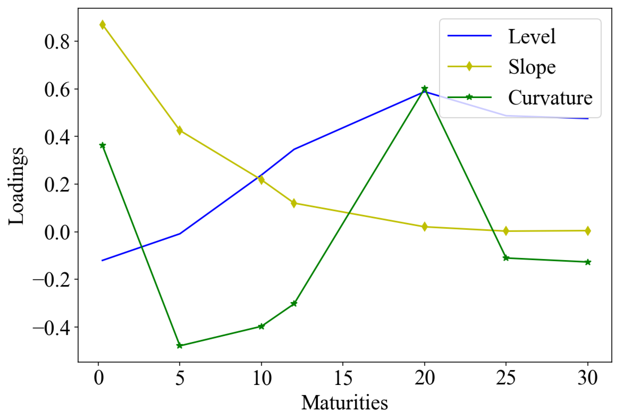
Figure 2.
3 months, 5, 10, 20, and 30 years observed yields on are plotted together with the spread between 5 and 20 years, against maturities. The 5 - 20 year spread is indicative of a slope while there are overlaps from one line to others suggesting either positive of inverted yields. Data were retrieved from Thomson Reuters.
Figure 2.
3 months, 5, 10, 20, and 30 years observed yields on are plotted together with the spread between 5 and 20 years, against maturities. The 5 - 20 year spread is indicative of a slope while there are overlaps from one line to others suggesting either positive of inverted yields. Data were retrieved from Thomson Reuters.
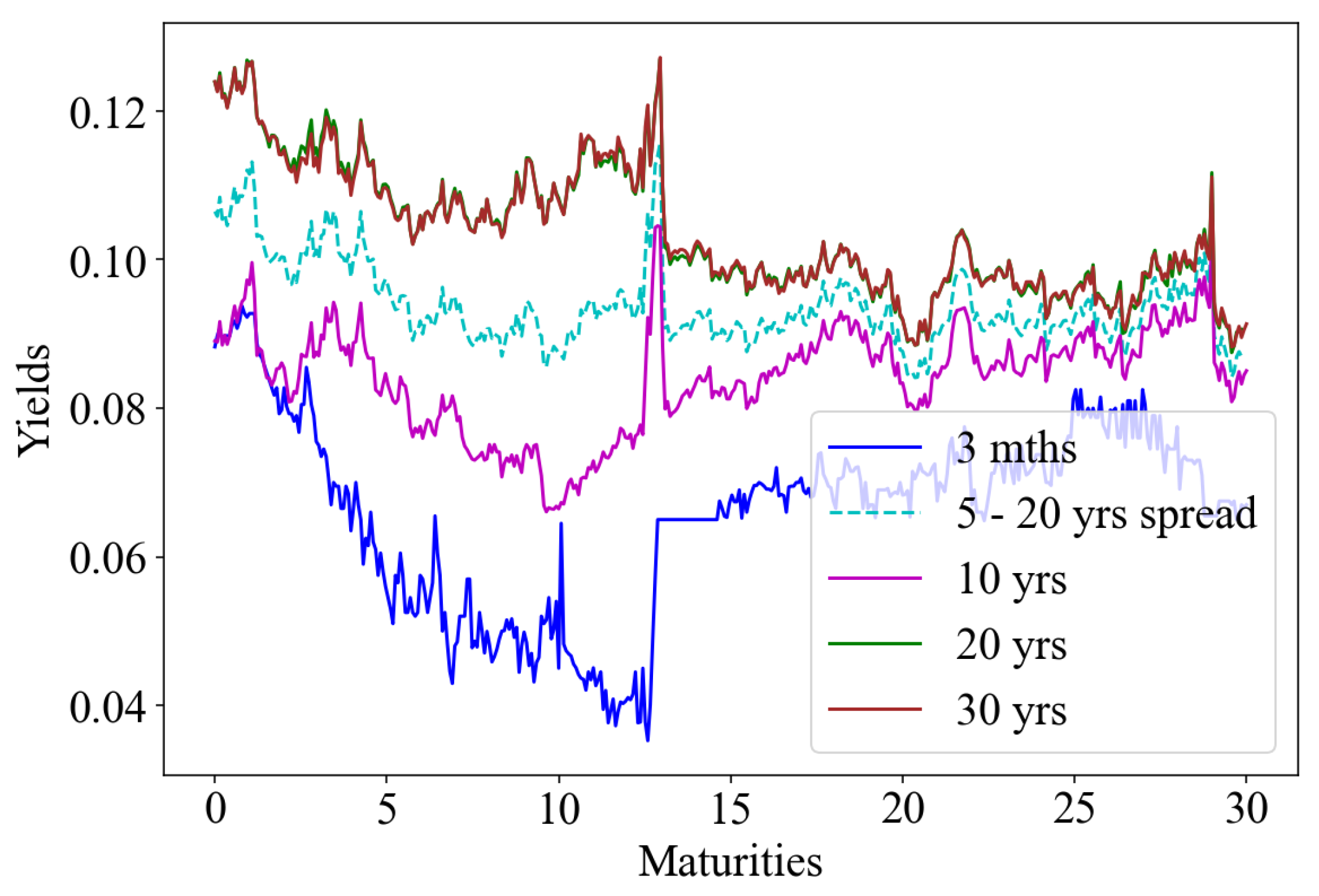
Figure 3.
(a) Factor 1 residuals. (b) Factor 2 residuals. (c) Factor 3 residuals. QQ-plots for the residuals derived from model computed factors and observed yields. For each factor the deviation of the red line from the blue exhibit asymmetry. The slight skewness in the residuals may not be alarming but does indicate that the models are not perfectly capturing the underlying distribution as confirmed generally by the stylised facts for asset returns. Data were retrieved from Thomson Reuters.
Figure 3.
(a) Factor 1 residuals. (b) Factor 2 residuals. (c) Factor 3 residuals. QQ-plots for the residuals derived from model computed factors and observed yields. For each factor the deviation of the red line from the blue exhibit asymmetry. The slight skewness in the residuals may not be alarming but does indicate that the models are not perfectly capturing the underlying distribution as confirmed generally by the stylised facts for asset returns. Data were retrieved from Thomson Reuters.
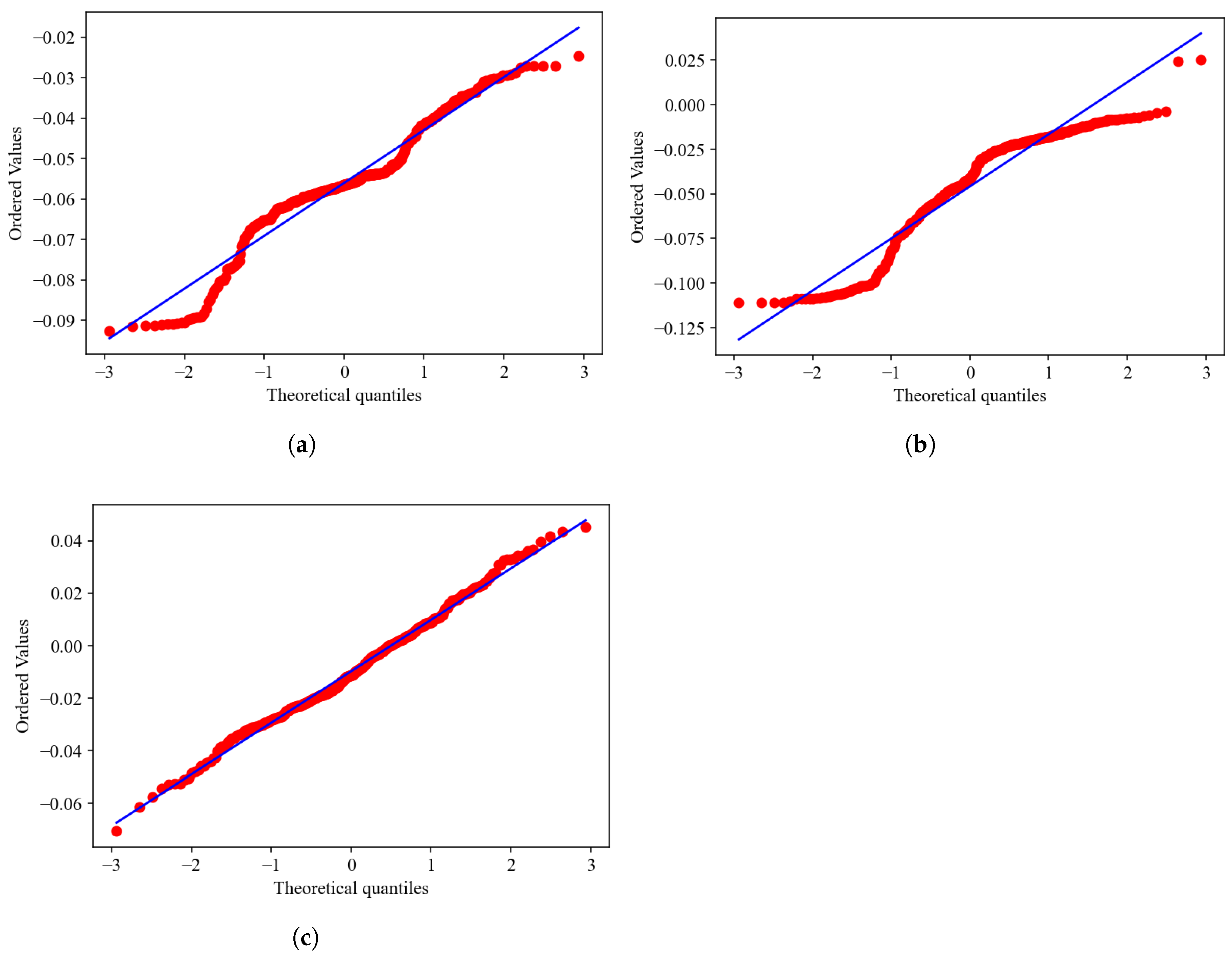
Figure 4.
(a) Factor 1 residuals. (b) Factor 2 residuals. (c) Factor 3 residuals. QQ-plots for the residuals derived from models computed factors and observed yields. For each factor the deviation of the red line from the blue exhibit asymmetry. The slight skewness in the residuals may not be alarming but does indicate that the models are not perfectly capturing the underlying distribution as confirmed generally by the stylised facts for asset returns. Data were retrieved from Thomson Reuters.
Figure 4.
(a) Factor 1 residuals. (b) Factor 2 residuals. (c) Factor 3 residuals. QQ-plots for the residuals derived from models computed factors and observed yields. For each factor the deviation of the red line from the blue exhibit asymmetry. The slight skewness in the residuals may not be alarming but does indicate that the models are not perfectly capturing the underlying distribution as confirmed generally by the stylised facts for asset returns. Data were retrieved from Thomson Reuters.
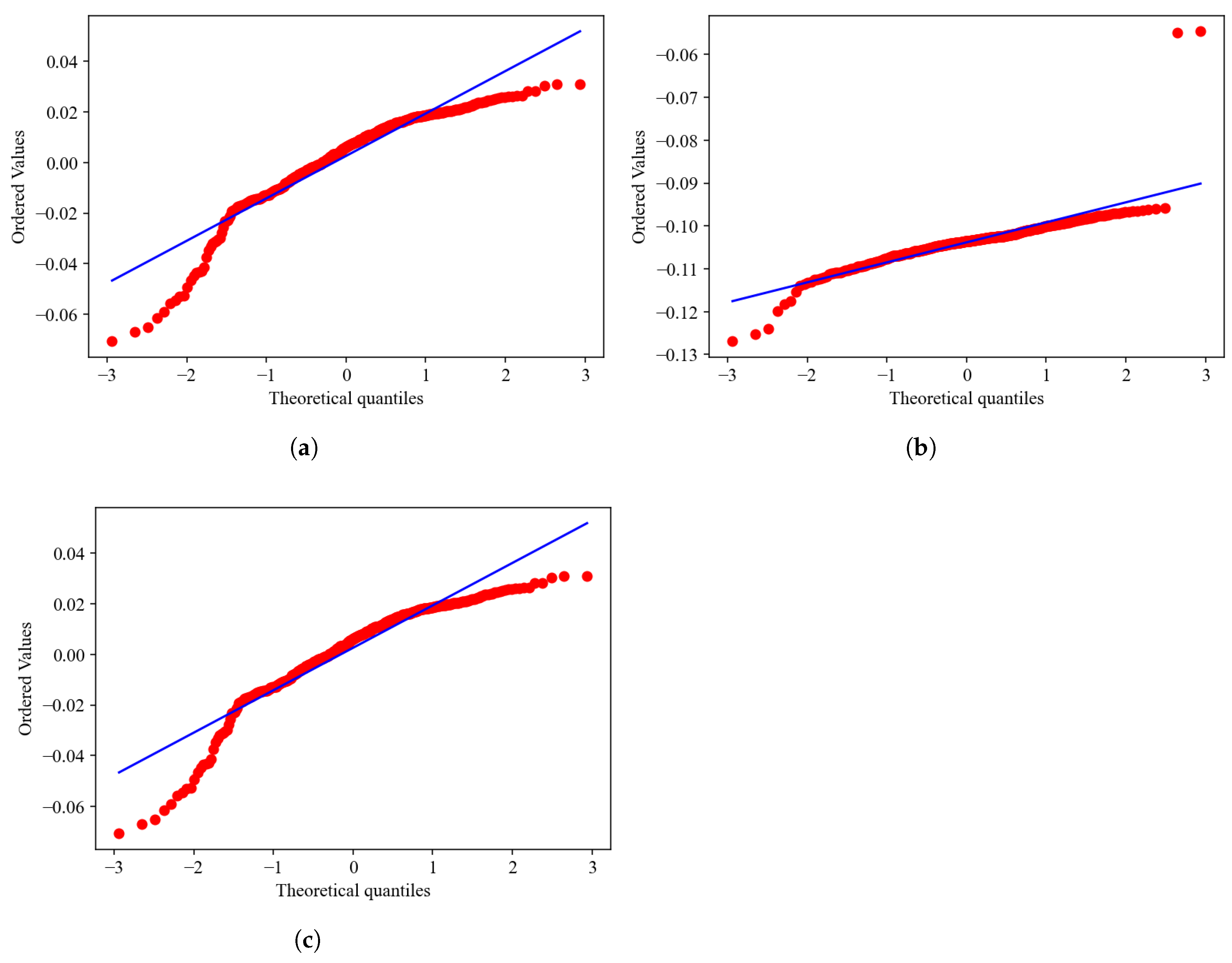
Figure 5.
Model-implied instantaneous rate in percentages is plotted against maturities. and appear in blue and magenta colours, respectively. Data were retrieved from Thomson Reuters.
Figure 5.
Model-implied instantaneous rate in percentages is plotted against maturities. and appear in blue and magenta colours, respectively. Data were retrieved from Thomson Reuters.
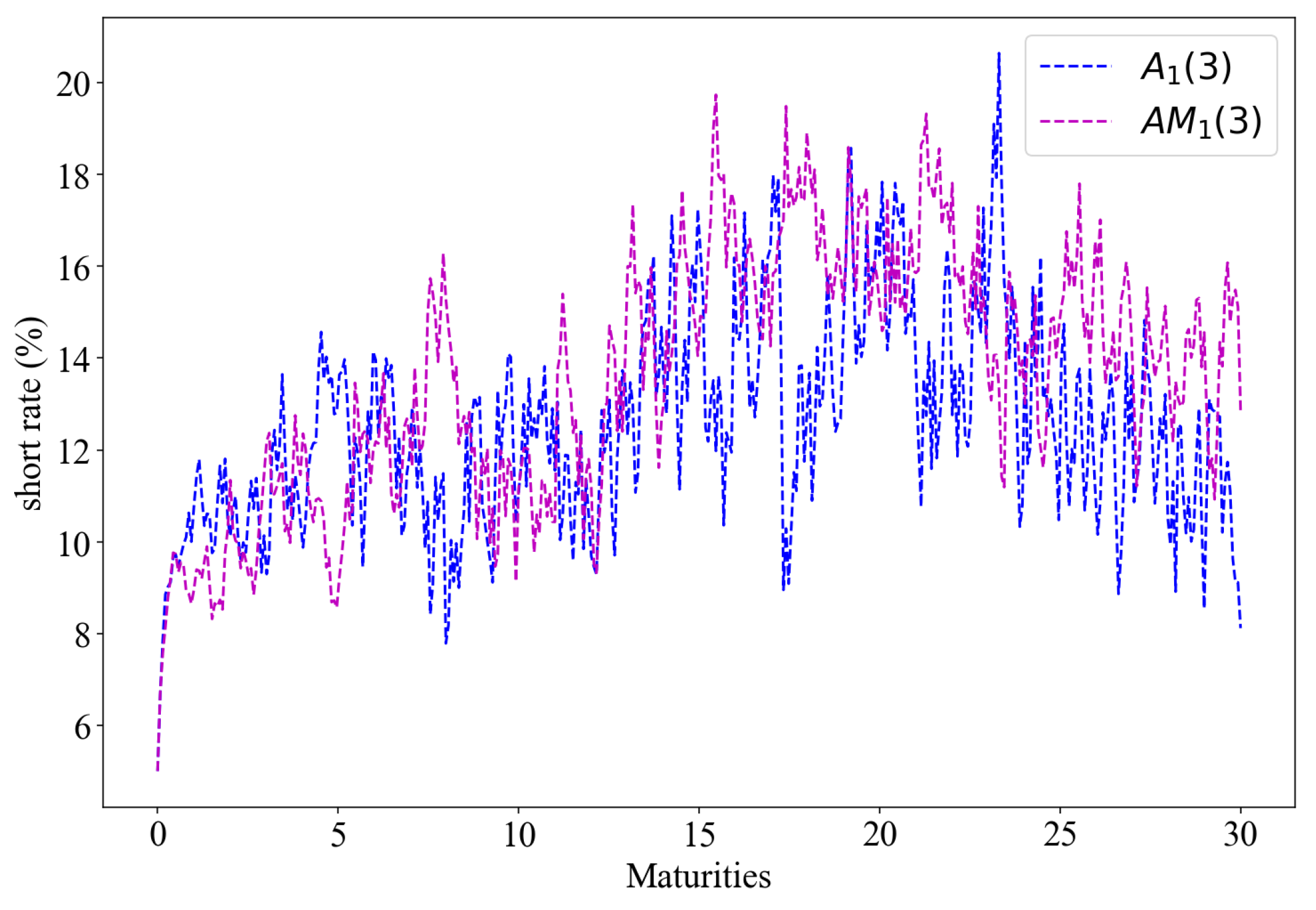
Figure 6.
Model-implied instantaneous rate in percentages is plotted against maturities. and appear in blue and magenta colours, respectively. Data were retrieved from Thomson Reuters.
Figure 6.
Model-implied instantaneous rate in percentages is plotted against maturities. and appear in blue and magenta colours, respectively. Data were retrieved from Thomson Reuters.
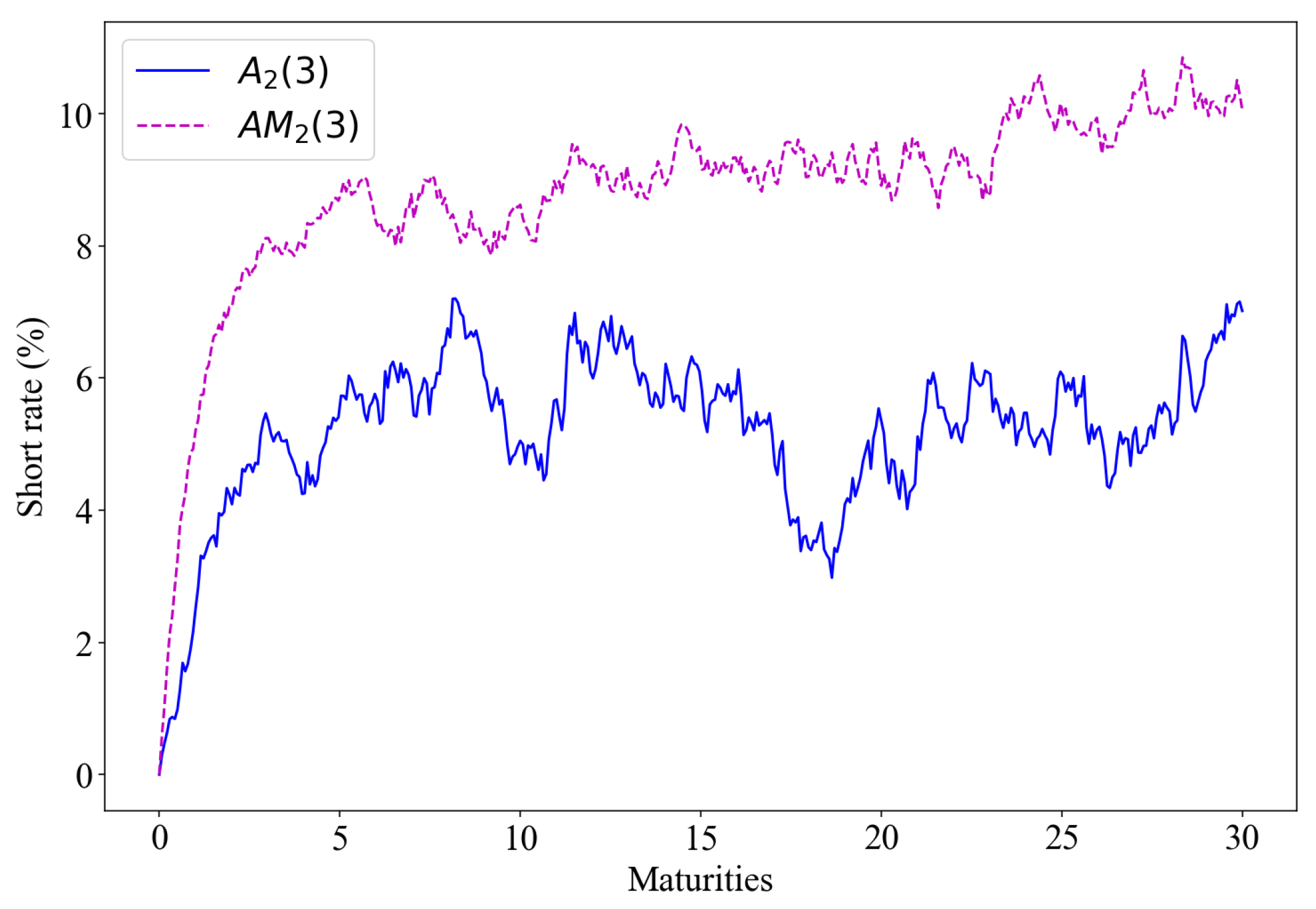

Table 1.
Statistical summary of in-sample yields for the SA Treasury bond by maturity caption. Data were retrieved from Thomson Reuters.
Table 1.
Statistical summary of in-sample yields for the SA Treasury bond by maturity caption. Data were retrieved from Thomson Reuters.
| 3 mths | 5 yrs | 10 yrs | 12 yrs | 20 yrs | 25 yrs | 30 yrs | |
|---|---|---|---|---|---|---|---|
| count | 418 | 418 | 418 | 418 | 418 | 418 | 418 |
| mean | 0.066 | 0.084 | 0.094 | 0.098 | 0.103 | 0.104 | 0.104 |
| std | 0.013 | 0.007 | 0.006 | 0.007 | 0.011 | 0.009 | 0.009 |
| min | 0.035 | 0.066 | 0.084 | 0.085 | 0.000 | 0.088 | 0.088 |
| 25% | 0.058 | 0.080 | 0.090 | 0.093 | 0.097 | 0.097 | 0.097 |
| 50% | 0.069 | 0.085 | 0.092 | 0.096 | 0.101 | 0.101 | 0.101 |
| 75% | 0.074 | 0.089 | 0.096 | 0.101 | 0.110 | 0.111 | 0.110 |
| max | 0.094 | 0.105 | 0.117 | 0.122 | 0.127 | 0.127 | 0.127 |
| skew | -0.406 | -0.361 | 1.162 | 0.939 | -3.232 | 0.561 | 0.583 |
| kurtosis | -0.278 | 0.116 | 1.349 | 0.633 | 30.693 | -0.536 | -0.457 |
Table 2.
Correlation matrix of in-sample yields across maturities. Data were retrieved from Thomson Reuters.
Table 2.
Correlation matrix of in-sample yields across maturities. Data were retrieved from Thomson Reuters.
| 3 mths | 5 yrs | 10 yrs | 12 yrs | 20 yrs | 25 yrs | 30 yrs | |
|---|---|---|---|---|---|---|---|
| 3 mths | 1.000 | 0.713 | 0.302 | 0.046 | -0.111 | -0.152 | -0.152 |
| 5 yrs | 0.713 | 1.000 | 0.613 | 0.269 | -0.035 | -0.063 | -0.051 |
| 10 yrs | 0.302 | 0.613 | 1.000 | 0.918 | 0.608 | 0.718 | 0.724 |
| 12 yrs | 0.046 | 0.269 | 0.918 | 1.000 | 0.781 | 0.931 | 0.934 |
| 20 yrs | -0.111 | -0.035 | 0.608 | 0.781 | 1.000 | 0.838 | 0.836 |
| 25 yrs | -0.152 | -0.063 | 0.718 | 0.931 | 0.838 | 1.000 | 0.999 |
| 30 yrs | -0.152 | -0.051 | 0.724 | 0.934 | 0.836 | 0.999 | 1.000 |
Table 3.
The estimators reported here are based on the log-likelihood computed from the Fourier inversion of the characteristic function of yields. Computation is based on variables , and of both the model-based and observed yields. Parameters in the first column are the same as those used in (23), second column are initial guesses while the 3rd and 4th columns are calibrated from the models and , respectively. Figures in square brackets refer to initial parameter values which are restricted to zero in terms of the model assumptions.
Table 3.
The estimators reported here are based on the log-likelihood computed from the Fourier inversion of the characteristic function of yields. Computation is based on variables , and of both the model-based and observed yields. Parameters in the first column are the same as those used in (23), second column are initial guesses while the 3rd and 4th columns are calibrated from the models and , respectively. Figures in square brackets refer to initial parameter values which are restricted to zero in terms of the model assumptions.
| Parameter | Initial | Estimates | |
|---|---|---|---|
| 0.365 | 0.365 | 0.366 | |
| 0.015 | 0.015 | 0.008 | |
| 0.000 | 0.000 | 0.000 | |
| 0.083 | 0.083 | 0.083 | |
| 0.000 | 0.000 | 0.000 | |
| 0.000 | 0.000 | ||
| 4.270 | 4.275 | 4.212 | |
| 0.000 | 0.0213 | ||
| -0.094 | -0.094 | -0.089 | |
| -3.420 | -3.509 | -3.786 | |
| 0.000 | 0.000 | ||
| 0.000 | 0.035 | ||
| 17.400 | 17.421 | 18.006 | |
| 0.050 | 0.050 | 0.047 | |
| 0.050 | 0.050 | 0.050 | |
| 0.481 | 0.483 | 0.484 | |
| 0.666 | 0.666 | 0.669 | |
| 0.884 | 0.883 | 0.887 | |
| 0 | 0.000 | ||
| 0.025 | 0.000 | ||
| 0.233 | 0.0442 | ||
| AIC | -866.21 | -866.33 | |
| BIC | -769.36 | -769.48 | |
| Degree of freedom | 389 | 393 | |
| Critical value at 95% confidence level | 435.99 | 440.22 | |
| 57.16 | 87.57 | ||
| P-value | 1 | 1 | |
| Log-ikelihood function | -456.96 | -457.02 | |
| Iterations | 1498 | 1376 | |
Table 4.
The estimators reported here are based on the log-likelihood computed from the Fourier inversion of the characteristic function of yields. Computaion is based on moment labels , and of both the model-based and observed yields. Parameters in the first column are the same as those used in (23), second column are initial guesses while the 3rd and 4th columns are calibrated from the models and , respectively. Figures in square brackets refer to initial parameter values which are restricted to zero in terms of the model assumptions.
Table 4.
The estimators reported here are based on the log-likelihood computed from the Fourier inversion of the characteristic function of yields. Computaion is based on moment labels , and of both the model-based and observed yields. Parameters in the first column are the same as those used in (23), second column are initial guesses while the 3rd and 4th columns are calibrated from the models and , respectively. Figures in square brackets refer to initial parameter values which are restricted to zero in terms of the model assumptions.
| Parameter | Initial | Estimates | |
|---|---|---|---|
| 0.636 | 0.634 | 0.292 | |
| -33.900 | -33.989 | -12.427 | |
| -35.300 | -35.393 | -274.799 | |
| 0.000 | 0.000 | -0.002 | |
| 0.000 | 3.561 | ||
| 2.700 | 2.708 | 3.539 | |
| 0.000 | 0.000 | 0.000 | |
| 0.026 | 0.027 | 0.014 | |
| 0.026 | 0.026 | 0.053 | |
| -182.000 | -182.420 | -133.403 | |
| 0.000 | 1.001 | ||
| 0.000 | 0.000 | 0.095 | |
| 0.000 | 0.000 | 0.000 | |
| 0.003 | 0.003 | 0.002 | |
| 0.000 | 0.000 | ||
| 0.000 | 0.000 | ||
| 0.050 | 0.050 | 0.050 | |
| 0.496 | 0.495 | 0.496 | |
| 0.314 | 0.315 | 0.315 | |
| 0.626 | 0.628 | 0.628 | |
| 0.000 | 0.000 | ||
| -2.603 | 0.000 | ||
| 0.235 | 0.796 | ||
| AIC: | -3455.43 | -4483.99 | |
| BIC: | -3350.51 | -4379.07 | |
| Degree of freedom | 387 | 391 | |
| Critical value at 95% confidence | 433.87 | 438.11 | |
| statistic: | 77.26 | 96.01 | |
| P-value: | 1 | 1 | |
| Degrees of Freedom: | 391 | 391 | |
| Log-likelihood function | -1753.71 | -2267.99 | |
| Iterations | 1574 | 1471 | |
Table 5.
Average short rates, standard deviations and weekly volatilities for the observed three-month maturity are compared to the model-implied short rate averages, standard deviation and weekly volatilities for , and their maximal counterparts. Model-implied instantaneous rates were computed from (22) and (25).
Table 5.
Average short rates, standard deviations and weekly volatilities for the observed three-month maturity are compared to the model-implied short rate averages, standard deviation and weekly volatilities for , and their maximal counterparts. Model-implied instantaneous rates were computed from (22) and (25).
| Observed | |||||
|---|---|---|---|---|---|
| mean | 0.066 | 0.119 | 0.081 | 0.051 | 0.089 |
| std deviation | 0.013 | 0.028 | 0.019 | 0.010 | 0.015 |
| weekly volatility | 0.094 | 0.203 | 0.139 | 0.073 | 0.111 |
Table 6.
A comparison is made of the and models together with their maximal counterparts. Performance analysis results are presented in terms of statistical results of the model estimation based on the optimised parameters obtained from in-sample analysis.
Table 6.
A comparison is made of the and models together with their maximal counterparts. Performance analysis results are presented in terms of statistical results of the model estimation based on the optimised parameters obtained from in-sample analysis.
| AIC: | 77.37 | 77.45 | -52.71 | -58.28 |
| BIC: | 120.73 | 120.81 | -5.73 | -11.31 |
| df | 16 | 20 | 14 | 18 |
| 8.26 | 9.20 | 10.46 | 10.11 | |
| p-value | 1 | 1 | 0.73 | 0.93 |
| Log-likelihood | 14.69 | 14.73 | -52.35 | -55.14 |
| Iterations | 1447 | 1444 | 1532 | 1505 |
Disclaimer/Publisher’s Note: The statements, opinions and data contained in all publications are solely those of the individual author(s) and contributor(s) and not of MDPI and/or the editor(s). MDPI and/or the editor(s) disclaim responsibility for any injury to people or property resulting from any ideas, methods, instructions or products referred to in the content. |
© 2025 by the authors. Licensee MDPI, Basel, Switzerland. This article is an open access article distributed under the terms and conditions of the Creative Commons Attribution (CC BY) license (http://creativecommons.org/licenses/by/4.0/).
Copyright: This open access article is published under a Creative Commons CC BY 4.0 license, which permit the free download, distribution, and reuse, provided that the author and preprint are cited in any reuse.


