2. Materials and Methods
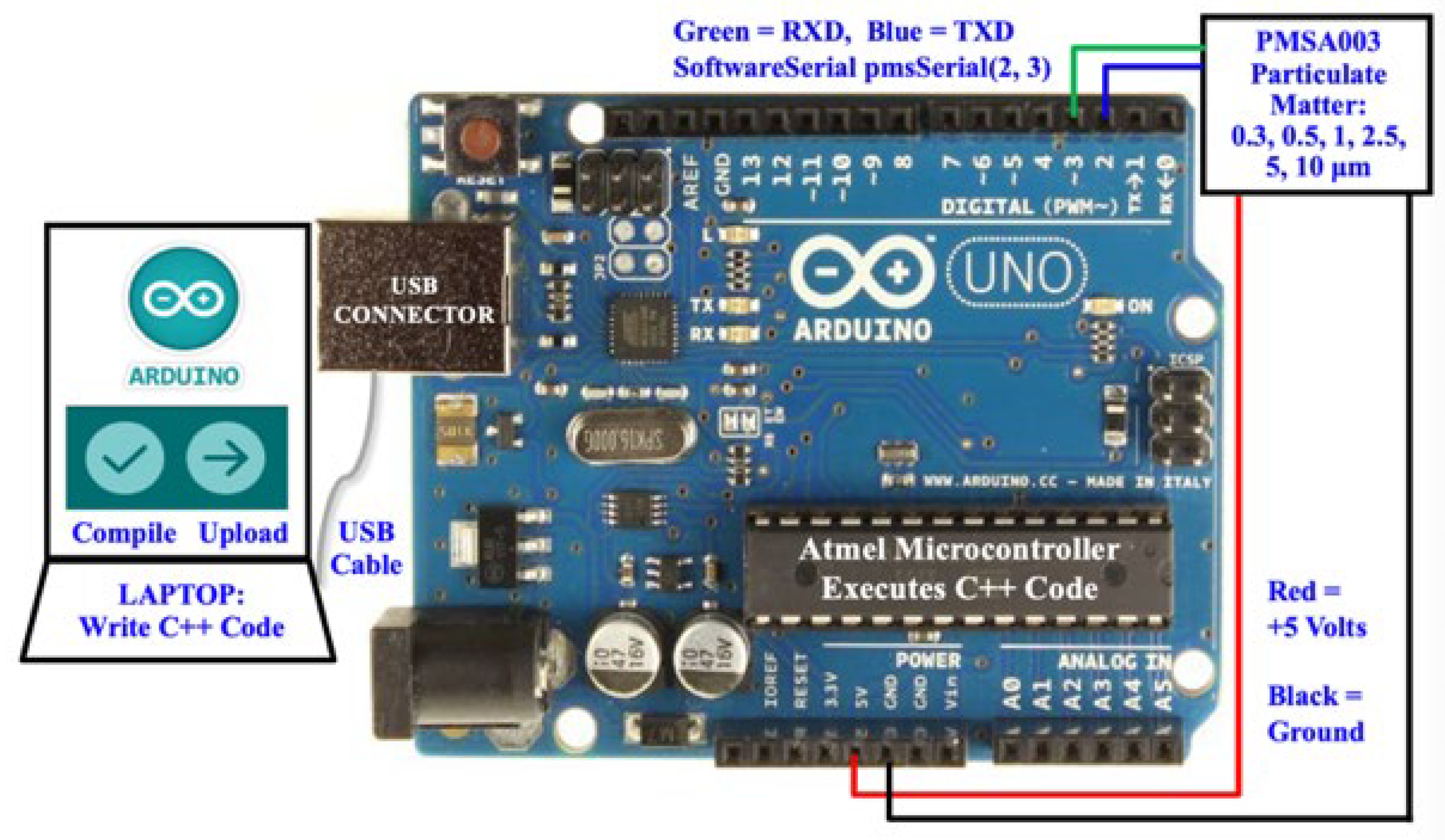
The research plan was to instrument an Arduino Uno [
3] with a PMS003 Air Monitoring Breakout sensor [
4],
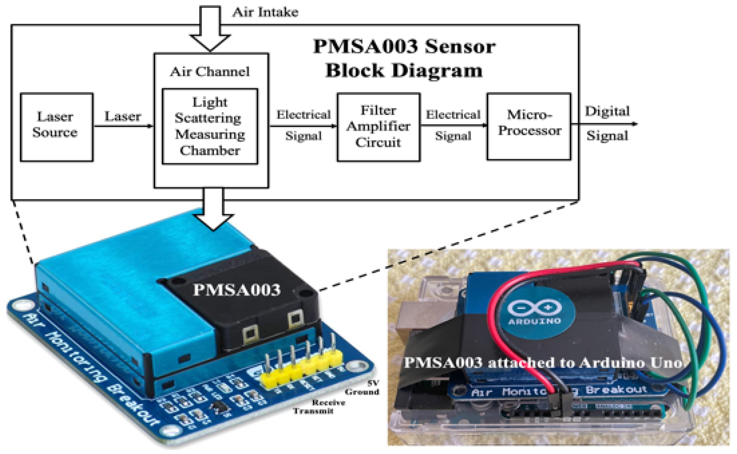
Figure 1. The PMSA003,
Figure 2, counts particulate matter in six diameters: 0.3, 0.5, 1, 2.5, 5, and 10 µm (micrometers) for a fixed volume of air, namely 0.1 Liters.
In
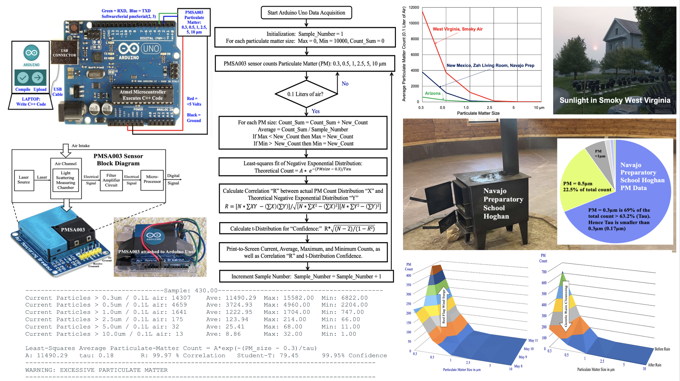
Figure 1, the wires were color coded as follows. Ground was black and +5 volts was red. The digital communications between the Arduino UNO and the PMSA003 particle counter were green for receive (RXD) and blue for transmit (TXD).
Figure 1 and
Figure 2 indicated that three computers were simultaneously linked to gather and process the experimental data, namely an Apple laptop, the Atmel Microcontroller on the Arduino UNO board (
Figure 1), and the microprocessor in the PMSA003 Particulate Matter sensor (
Figure 2).
The research plan then included programming the Arduino Uno to gather the particulate matter shown in
Table 1, tally the PM counts, calculate the average, maximum, and minimum of the PM counts, calculate the correlation “R” between the negative-exponential theoretical-model and the empirically measured PM counts, then calculate the confidence in that correlation R using the Student t-Distribution. One goal was to measure particulate matter in various locations in New Mexico, Arizona, and West Virginia, then to compare indoor particulate matter versus outdoor “free atmosphere” particulate matter. This study concluded with identifying dust generating events in our atmosphere, such as high winds generated by weather fronts, and dust scrubbing events, such as gentle rain.
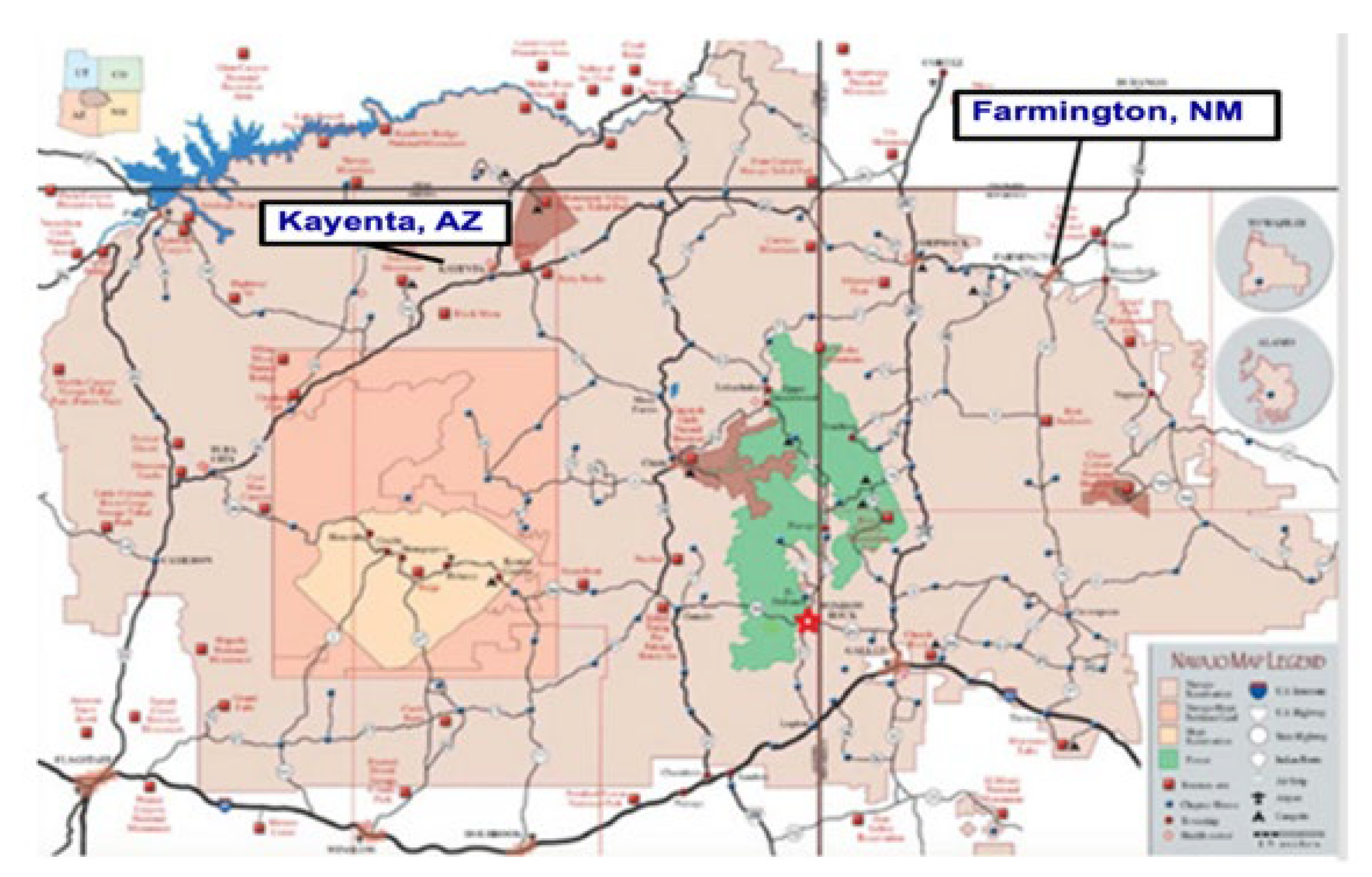
Figure 3 provides a map of the Navajo Nation [
5] which straddles Arizona, New Mexico, and Utah in the Four Corners region of the desert southwest. This area has a combination of desert such as the Painted Desert, and forests in the Chuska Mountains which go up to 10,000’ (3000m) in elevation.
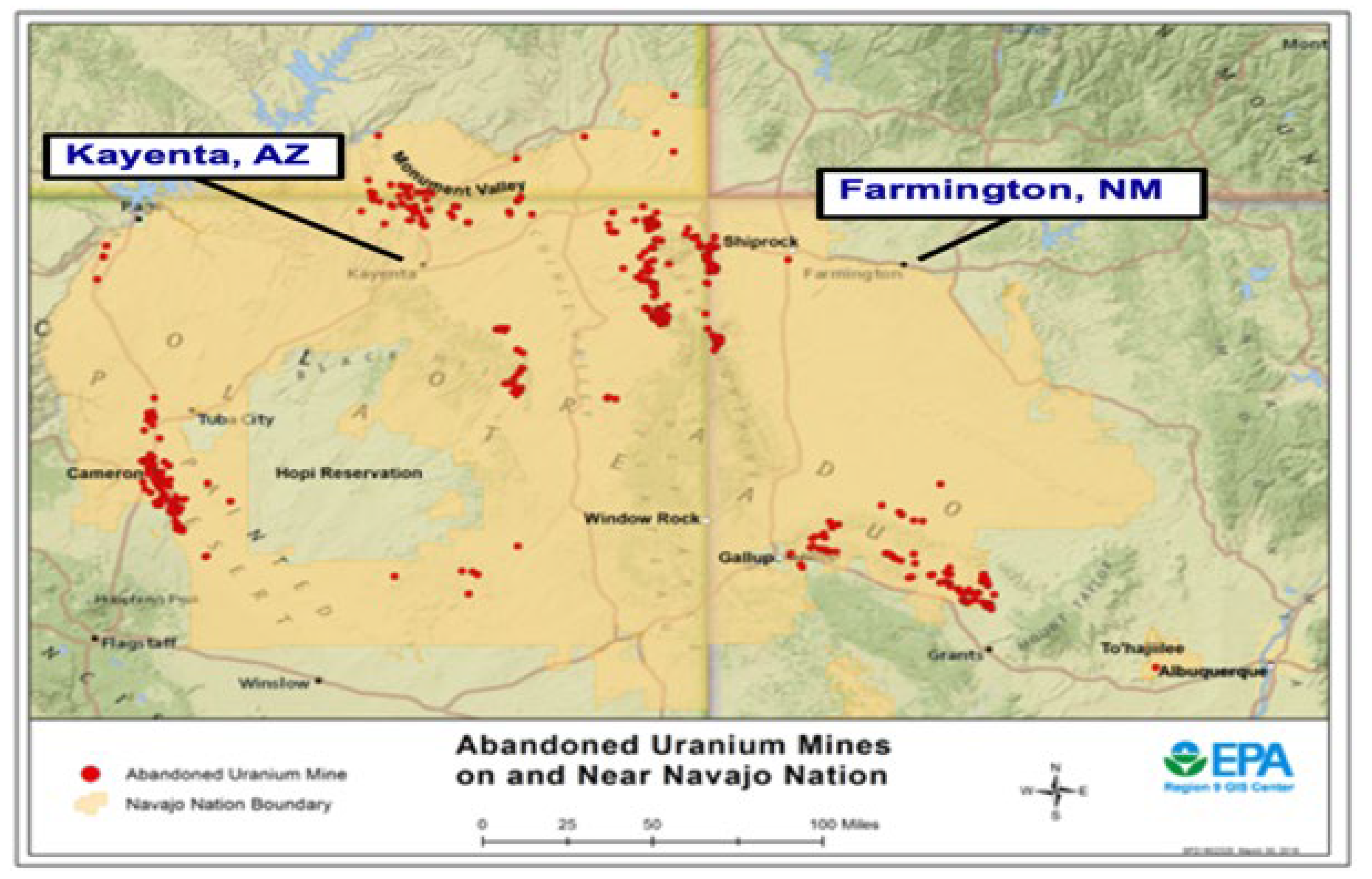
Figure 4, next page, details the locations of over 500 Abandoned Uranium Mines (AUMs) on the Navajo Nation, [
6]. Just east of Gallup, NM was the tragic Church Rock Uranium Spill [
7]. The Church Rock Uranium Mill Spill occurred in New Mexico on July 16, 1979, when United Nuclear Corporation’s uranium tailings disposal pond at its uranium mill in Church Rock breached its rock dam. This accident remains the largest release of radioactive material in U.S. history, having released more radioactivity than the Three Mile Island accident four months earlier. The uranium ores present in the tailings were made mobile by the same acids that ate through the rock retaining wall and allowed for a historic flood of radioactive material into the Navajo Nation. The released radioactivity combined with the area soil, resulting in mobile radioactive dust. Our reservation has 523 abandoned uranium mines (AUM) that are both remnants of the cold-war era and currently EPA Superfund Cleanup sites [
8].
Additionally, wood fired stoves in Hogans can release large amounts of particulate matter, due to incomplete combustion. Thus, it is critical to better understand the particulate matter across the Navajo Nation.
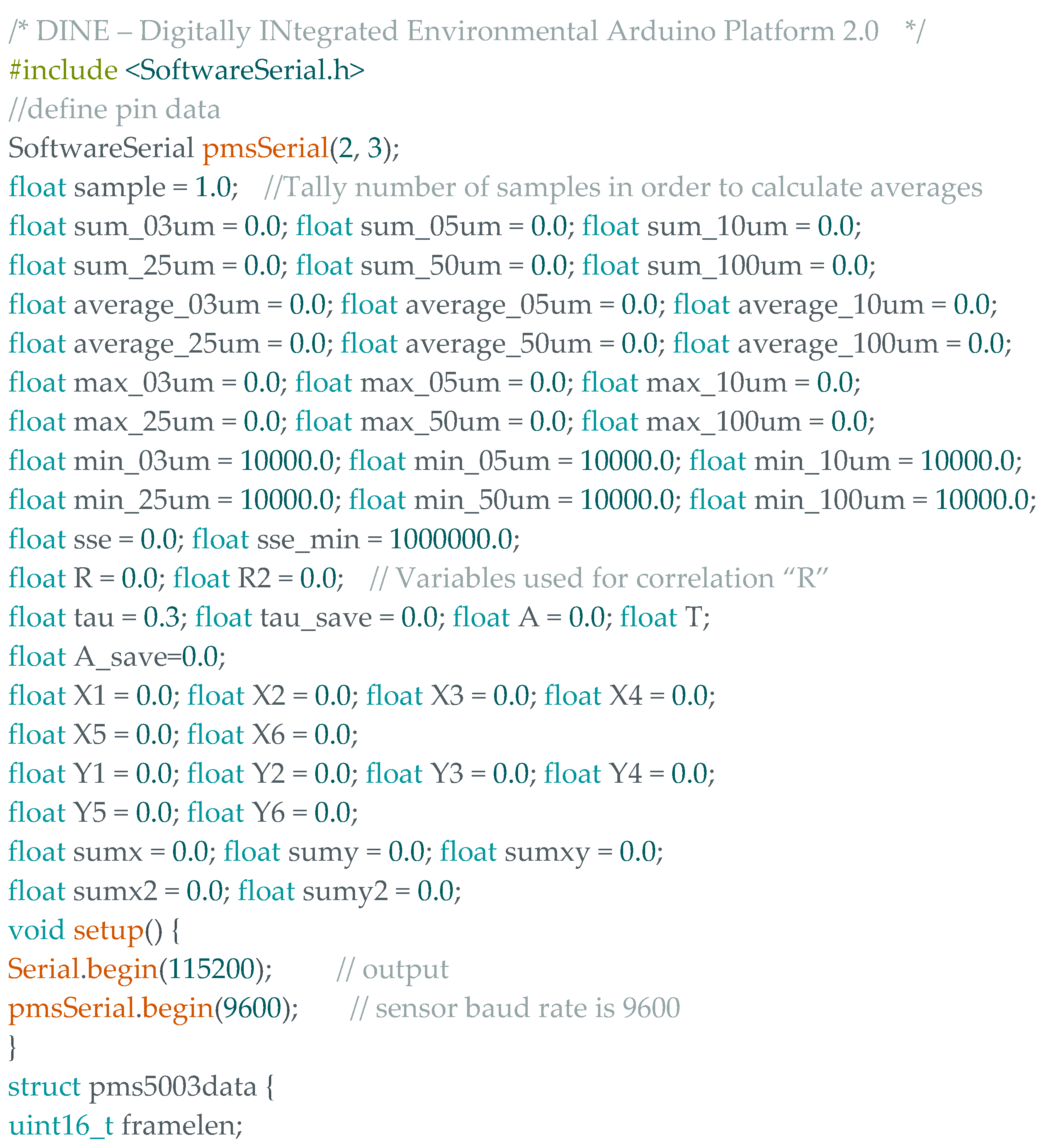
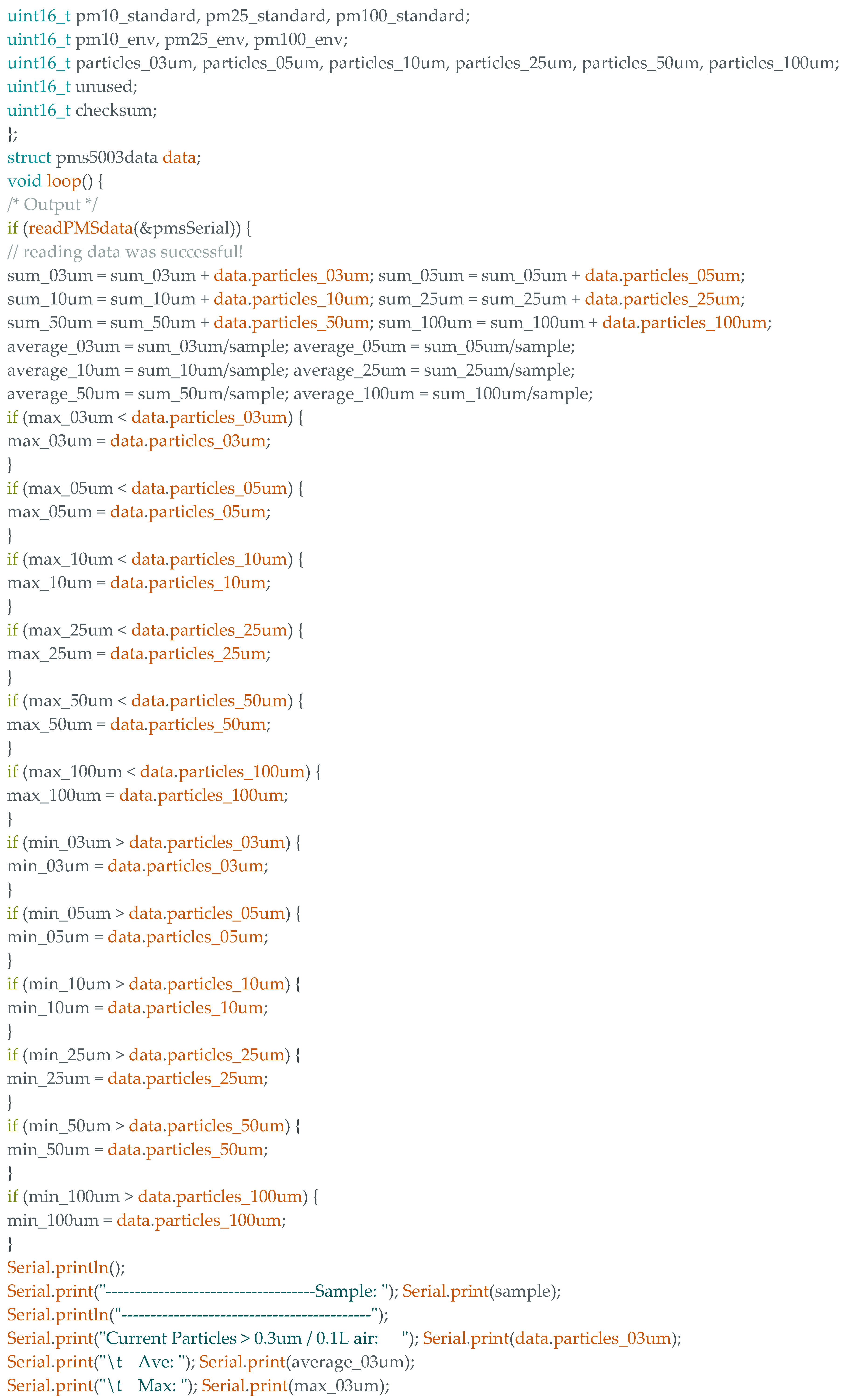
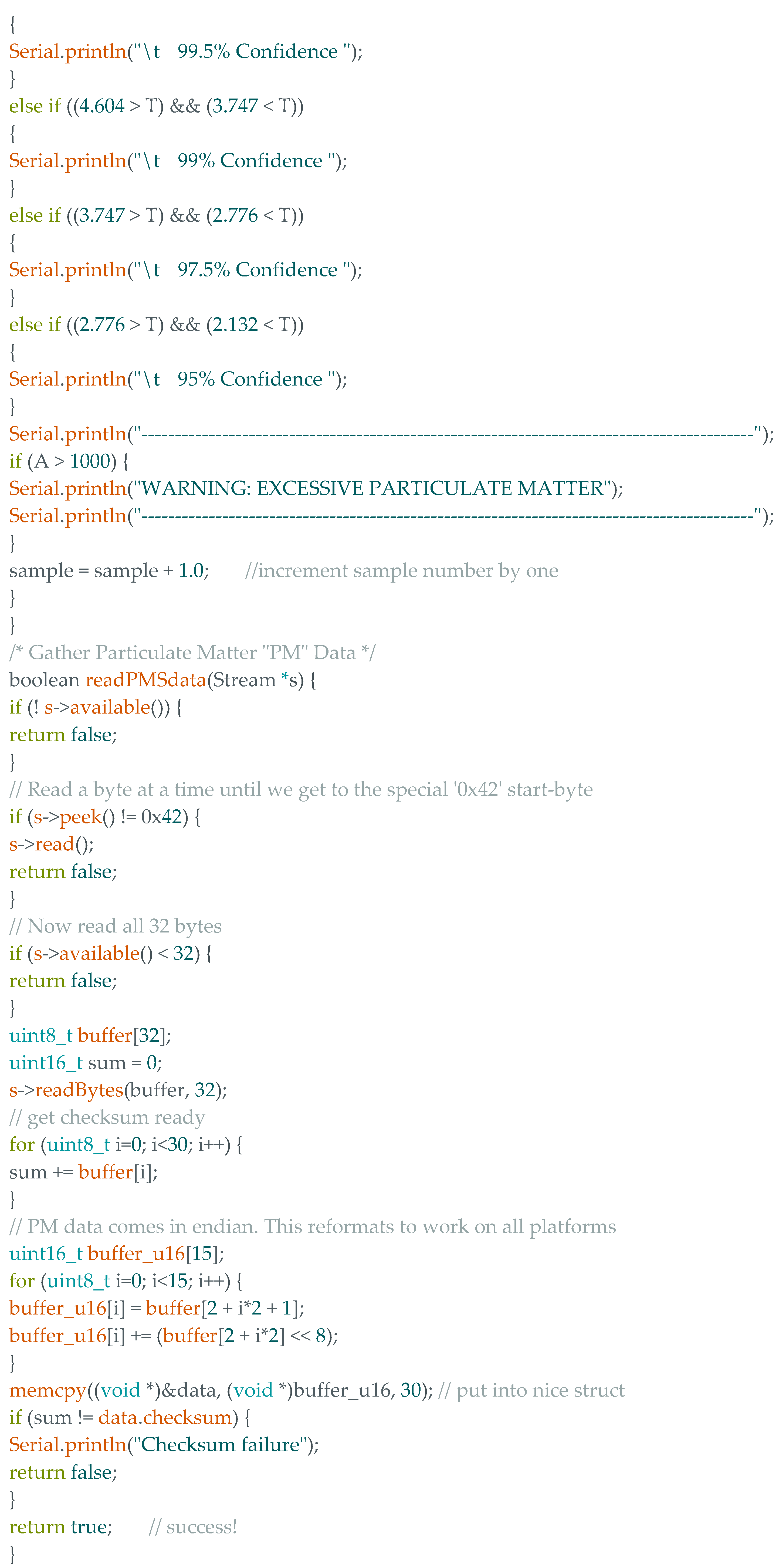
Particulate Matter sizes were collected via the Arduino Uno which executed the Arduino code, which is listed in
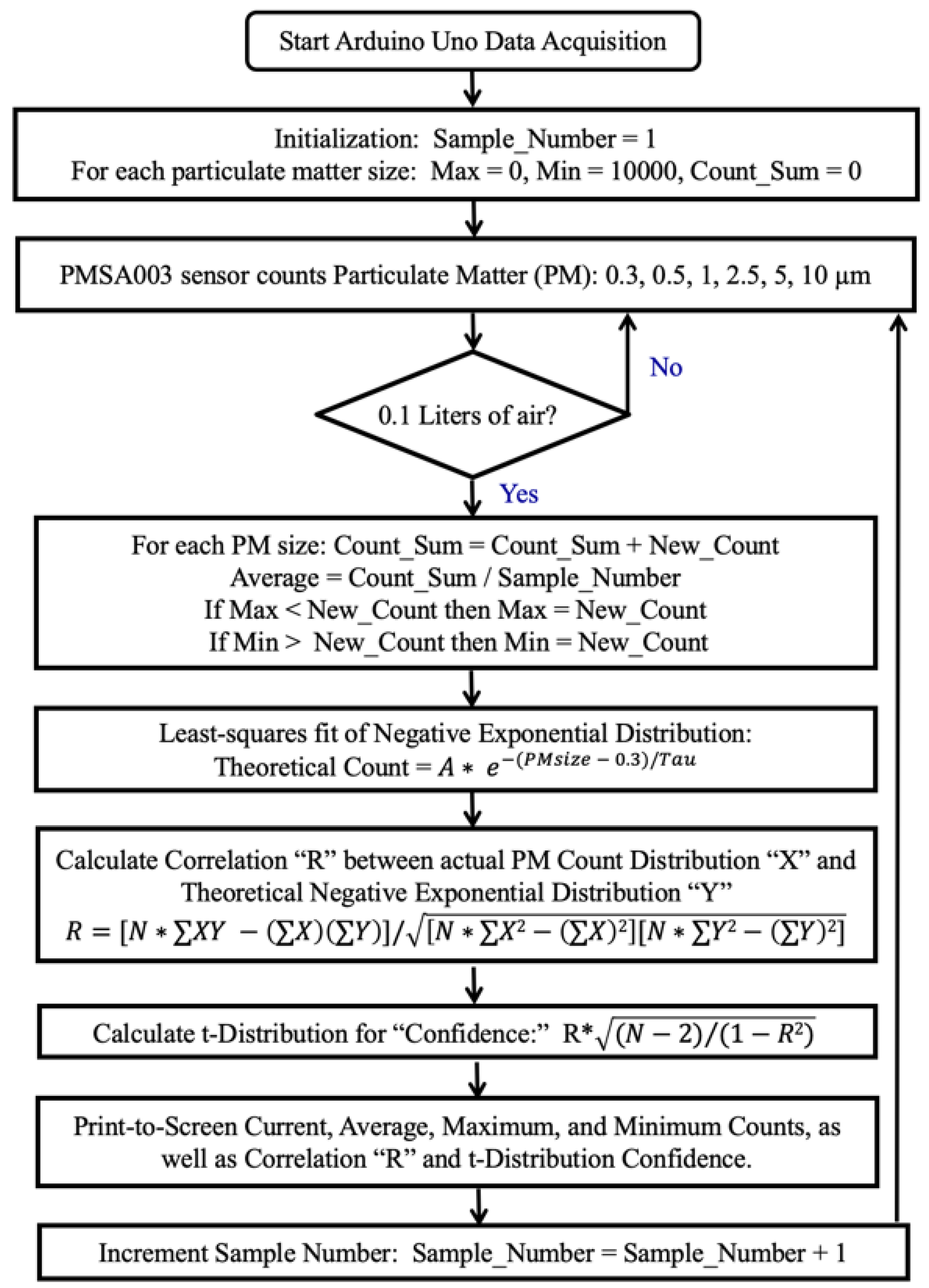
Appendix A. A flowchart of the data acquisition programming is shown in
Figure 5, on the next page. The data acquisition program begins with the initialization of key parameters. First of all, the Sample_Number is initialized to 1. Then, for each particulate matter size, the maximum count is set to zero, the minimum count is set to 10000, and the Count_Sum is set to 0.
The next step was the PMSA sensor counting particulate matter of the six sizes 0.3, 0.5, 1, 2.5, 5, and 10 µm. This process continued within the PMSA sensor until a volume of air of 0.1 Liters was reached, then the counts for that 0.1 Liter volume of air were transmitted to the Arduino UNO.
It may seem counterintuitive to initialize the maximum to a low number such as zero, but when samples come in with counts exceeding the current maximum, the maximum was reset to the value of that higher count, by the Arduino code executed within the Atmel microcontroller of the Arduino UNO.
Similarly, it may seem counterintuitive to initialize the minimum to a really high number such as 10000, but when samples come in with counts smaller than the current minimum, the minimum was reset to the value of that lower count, by the Arduino code executed within the Atmel microcontroller of the Arduino UNO. Thus, the Arduino UNO individually tracks the maximums and minimums of the six different particulate matter sizes, and adjusts those maximums and minimums as needed.
The New_Count information is added to the previous Count_Sum to create an updated Count_Sum. When the updated Count_Sum is divided by the Sample_Number, the average count for that particular particulate matter size is calculate.
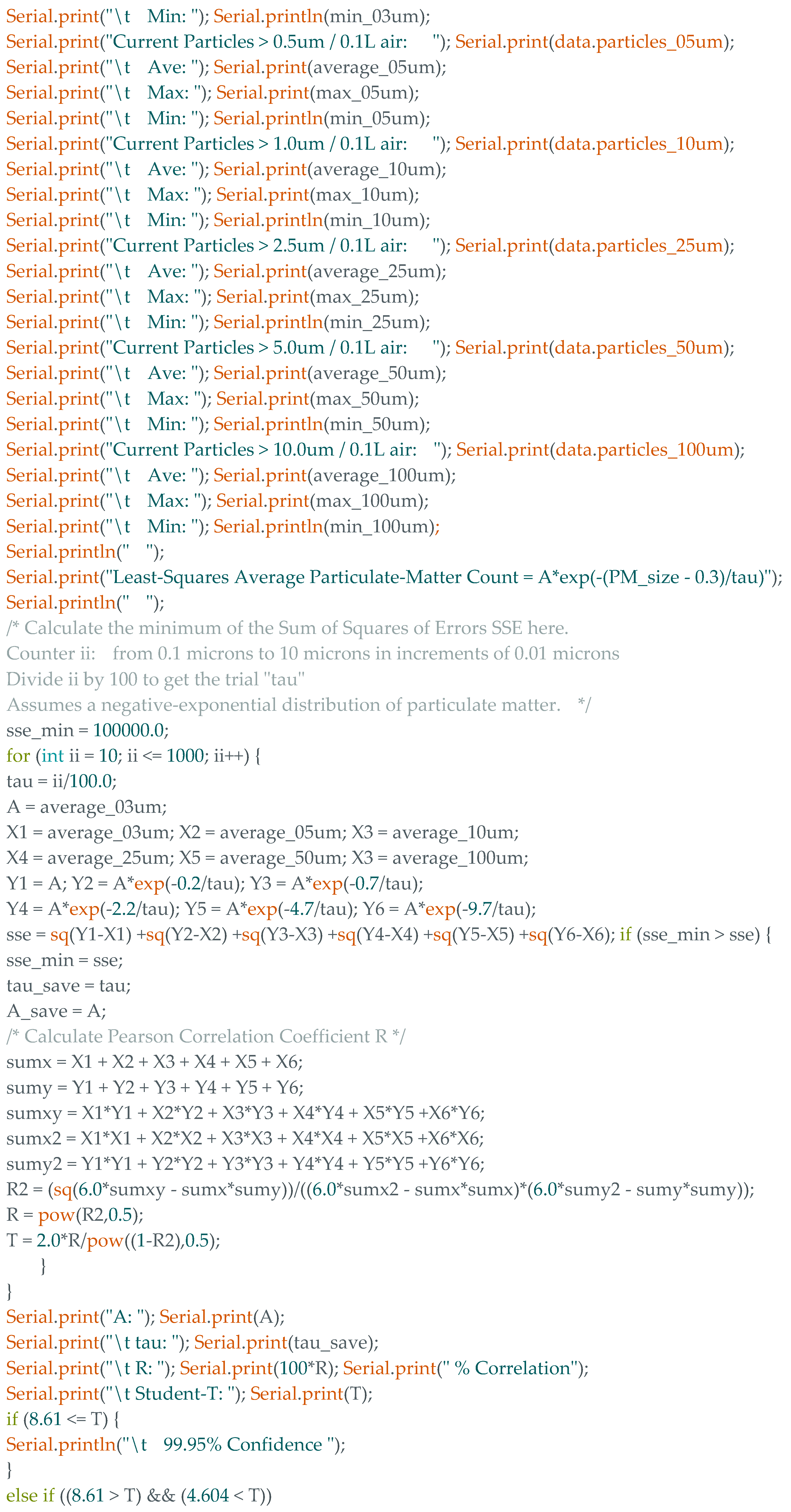
Then, the Arduino code within the Arduino UNO does a least-squares fit of our theoretical model within the Atmel microcontroller of the Arduino UNO. This theoretical model is a Negative Exponential Distribution:
After the least-squares fit, the Arduino code calculates the Correlation “R” between actual PM Count Distribution “X” and the Theoretical Negative Exponential Distribution “Y” with this equation, [
9]:
Finally, the Arduino code calculates the t-Distribution “T” to as part of the determination of the confidence in the correlation:
The confidence is a measure of the “believability” of the correlation R. The value of T is compared by the Arduino code to a tabulated “test” value of 8.61, based on a desired 99.95% confidence and 4 degrees-of-freedom, [
10]. The 4 degrees-of-freedom is calculated from N=6 particulate matter sizes (0.3, 0.5, 1. 2.5, 5, 10) from which 2 is subtracted. The number 2, which was subtracted from N=6 to get the degrees of freedom, represents the “Amount A” and Tau “63.2% percentile” constants which were least-squares fit by the Arduino code executed by the Arduino UNO.
The calculations done by the Arduino UNO for correlation “R” and the Student t-Distribution were confirmed by the use of Excel.
3. Results
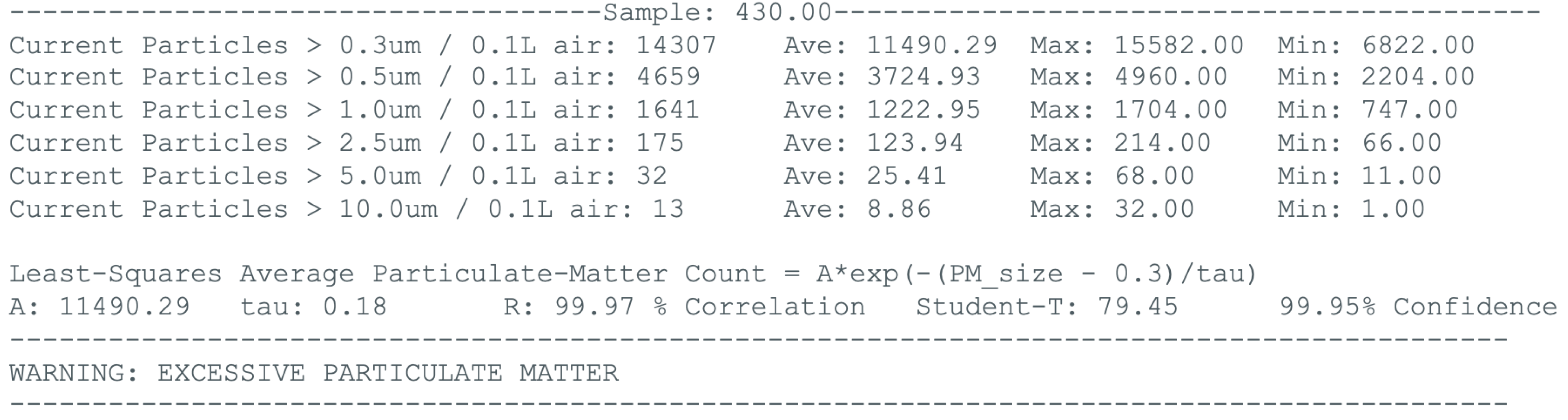
The PMSA003 particulate matter sensor counted particles of the sizes 0.3, 0.5, 1. 2.5, and 10 micrometers for an air volume of 0.1 Liters (100cc). The averages, maximums, and minimums of the above variables are calculated, as well as the least-squares fit of the theoretical Negative Exponential Distribution, the correlation “R” between the theoretical Negative Exponential Distribution, and the confidence in that correlation “R,” before all are printed to the screen of the attached laptop. The number of that sample were also printed to the laptop screen, as shown in
Figure 6. By clicking on the serial monitor icon in the upper right corner and selecting 115200 baud, the output display was shown.
After the above is example data was displayed, the Sample_Number is incremented by one and the processes cycles back to gather a new set of data from the PMSA003 Particulate Matter Sensor. Each new sample from the PMSA003 Particulate Matter Sensor updates the averages, maximums, minimums, correlation “R,” and Student t-Distribution. The above “Canadian-Fire Smoke” data in West Virginia was gathered during the summer-2023 Native Youth Climate Adaptation Leadership Conference (NYCALC). The AI (artificial intelligence) warning threshold in the Arduino UNO code was adjustable and could be selectively lowered for people with COPD (Chronic Obstructive Pulmonary Disease), asthma, allergies, etc.
3.1. INDOOR DATA – FARMINGTON, NM
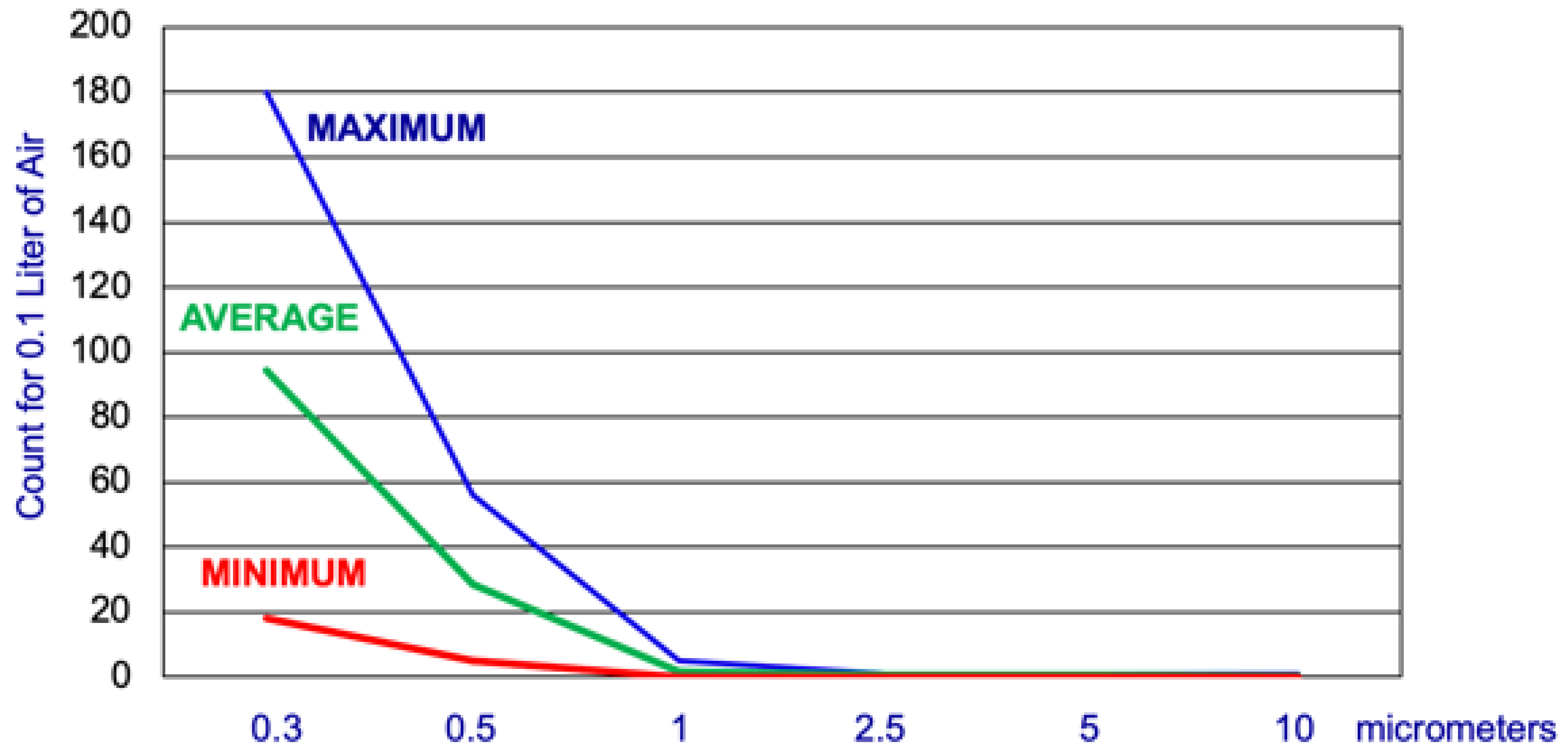
Figure 7 shows an example graph of particle count in 0.1 Liters of air versus particle size in micrometers, gathered inside the Bahe Dorm Room,
Table 2, of Navajo Preparatory School. Note the negative-exponential-like distribution of particle count versus particle size. The highest maximum, average, and minimum were for the 0.3 micrometer particles.
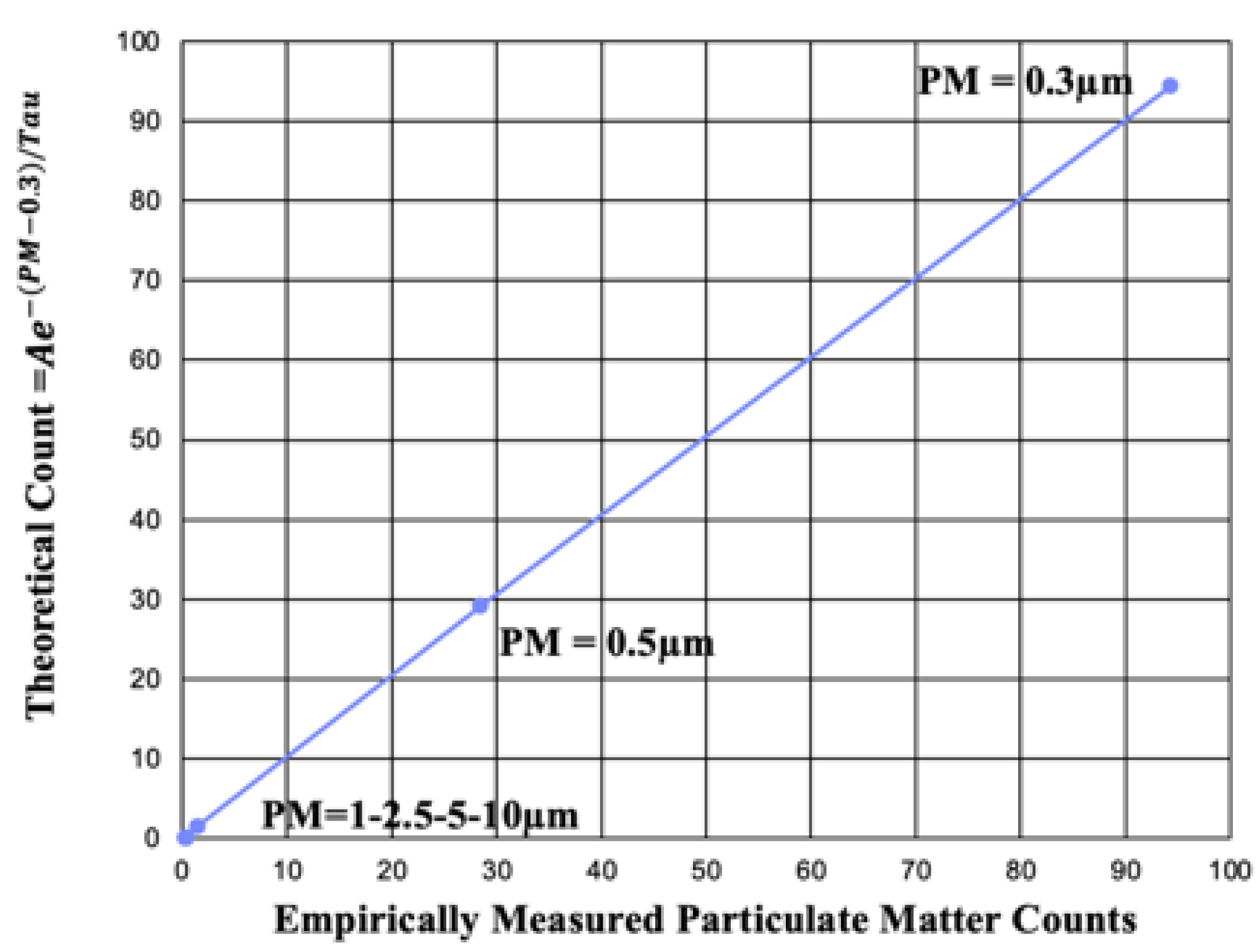
The equation used to model the average particle count in
Figure 7 was that of a negative exponential curve fit of the form: Theoretical Count =
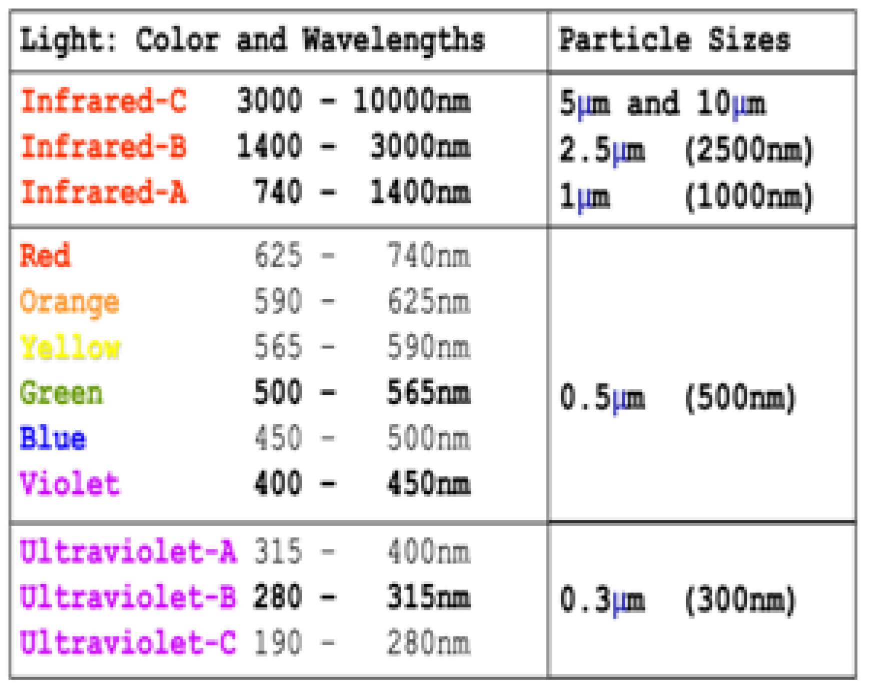
. The 0.3 term in the numerator of the exponential function was the smallest particle size detected. Using the =PEARSON function in EXCEL, a 99.99% correlation (100% is a perfect correlation) was calculated for the least-squares values of A = 94.33 and TAU = 0.17 micrometers. This least-squares calculation shows that the 63.2% (TAU) percentile constant is 0.17 micrometers, close to the wavelength of Ultraviolet-C,
Figure 9. Note: the argument of the exponential function needs to be unitless, and it is, because micrometers occur both in the numerator and denominator (µm/µm). Graphing the count from the negative exponential curve in
Figure 8 shows a nearly straight line (nearly perfect correlation).
Figure 9, above, compares the six particle sizes which were measured to wavelengths of light.
Table 2, below, lists the average particle count for six different particle sizes for all 12 indoor locations where data was obtained. Clearly, the carpeted Zah Living Room had an astoundingly large amount of particulate matter contamination.
Table 3, below, lists least-squares fit of TAU (63.2% percentile particle size, column 3) and the statistical correlations “R” (column 4) of the fit of the theoretical model of particle count: Theoretical Count =
and the empirical (experimental) data. The statistical correlations ”R” were amazingly high, between 99.08% and 99.99%. The confidence (column 5) is based on the T-Distribution for a sample size of N=6 different particle sizes, which gives 4 Degrees-Of-Freedom (DOF = N-2 = 4).
In
Table 3, the Degrees-Of-Freedom are 2 less than N=6 because there are two parameters in the theoretical model (Amount “A” and “Tau”). Calculated values of the T-Distribution (column 5) had a confidence of 99.95% confidence (T-test value = 8.61, [
9]) for all twelve indoor sites.
3.2. OUTDOOR DATA – TUCSON, ARIZONA WIND AND RAIN
Table 4, below, lists the average particle count for six different particle sizes for 9 different dates.
Table 5 then lists the least-squares fit of Amount “A,” Tau, correlation “R,” and the confidence in that correlation. Note how Tau (63.2% percentile) value in
Table 3 and
Table 5 are nearly equal.
3.3. WEST VIRGINIA SMOKY AIR
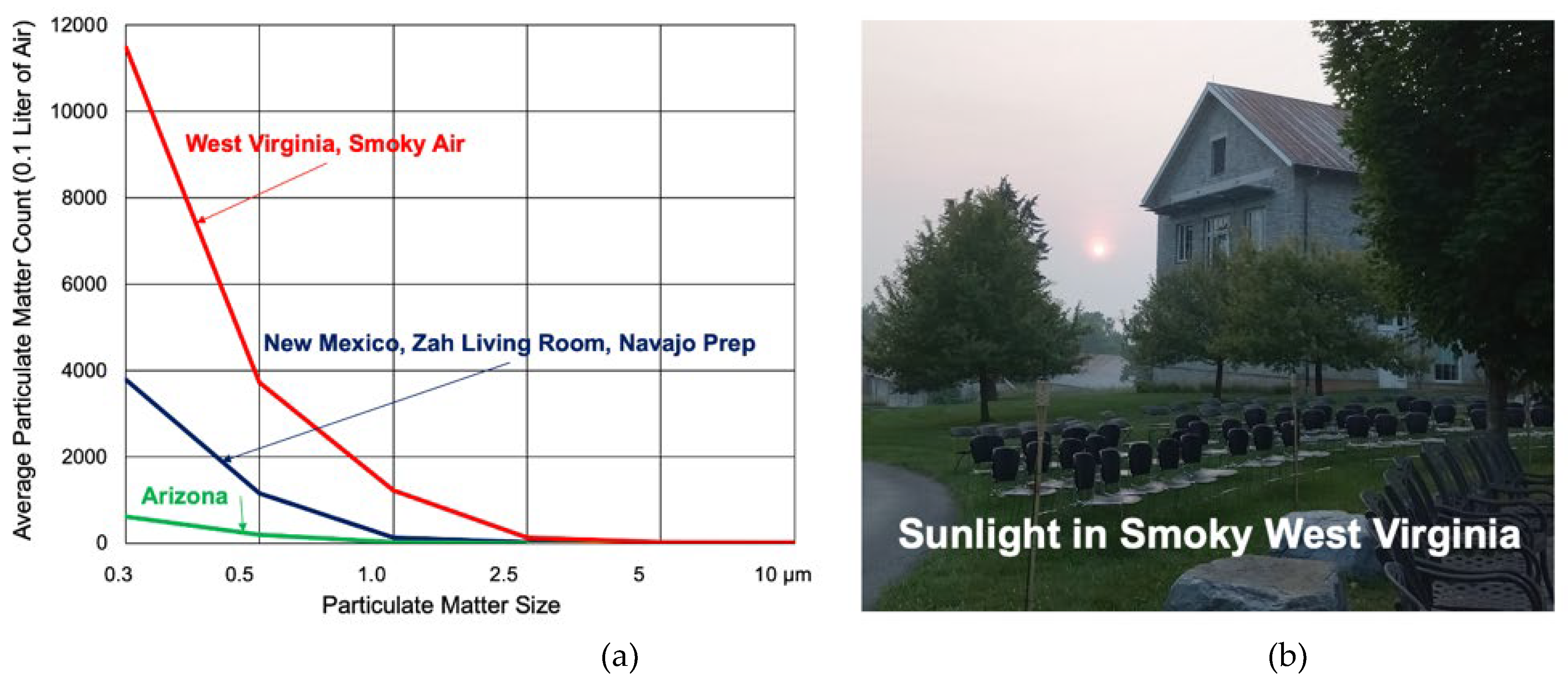
While the lead author attended the 2023 Native Youth Climate Adaptation Leadership Congress (NYCALC, through the Bureau of Indian Affairs) in West Virginia, she gathered the particulate matter data shown in
Table 6, during a particularly smoky day. This pervasive smoke was from the Canadian wildfires. The data in
Table 6 dwarfed the New Mexico data in
Table 3 and the Arizona data in
Table 5.
Table 7 then lists the least-squares fit of Amount “A,” Tau, correlation “R,” and the confidence in that correlation. Interestingly enough, Tables 3, 5, and 7 all had Tau (63.2% percentile) values between 0.15 and 0.18. The outdoor measurements were repeated 24 hour later, showing more than a 3X drop in particulate matter.
Figure 10 shows how much worse West Virginia was versus New Mexico and Arizona as well as how difficult it was to see the sun during daytime.
Figure 6 was created by the outdoor measurement,
Table 6 and
Table 7, July 29.
4. Discussion
It is interesting to compare “Tau,” the 63.2% percentile particle size, between the New Mexico measurements of
Table 3, the Arizona measurements of
Table 5, and the West Virginia measurements of
Table 7. Tau was never empirically measured. Instead, Tau is mathematically calculated by least-squares fit in
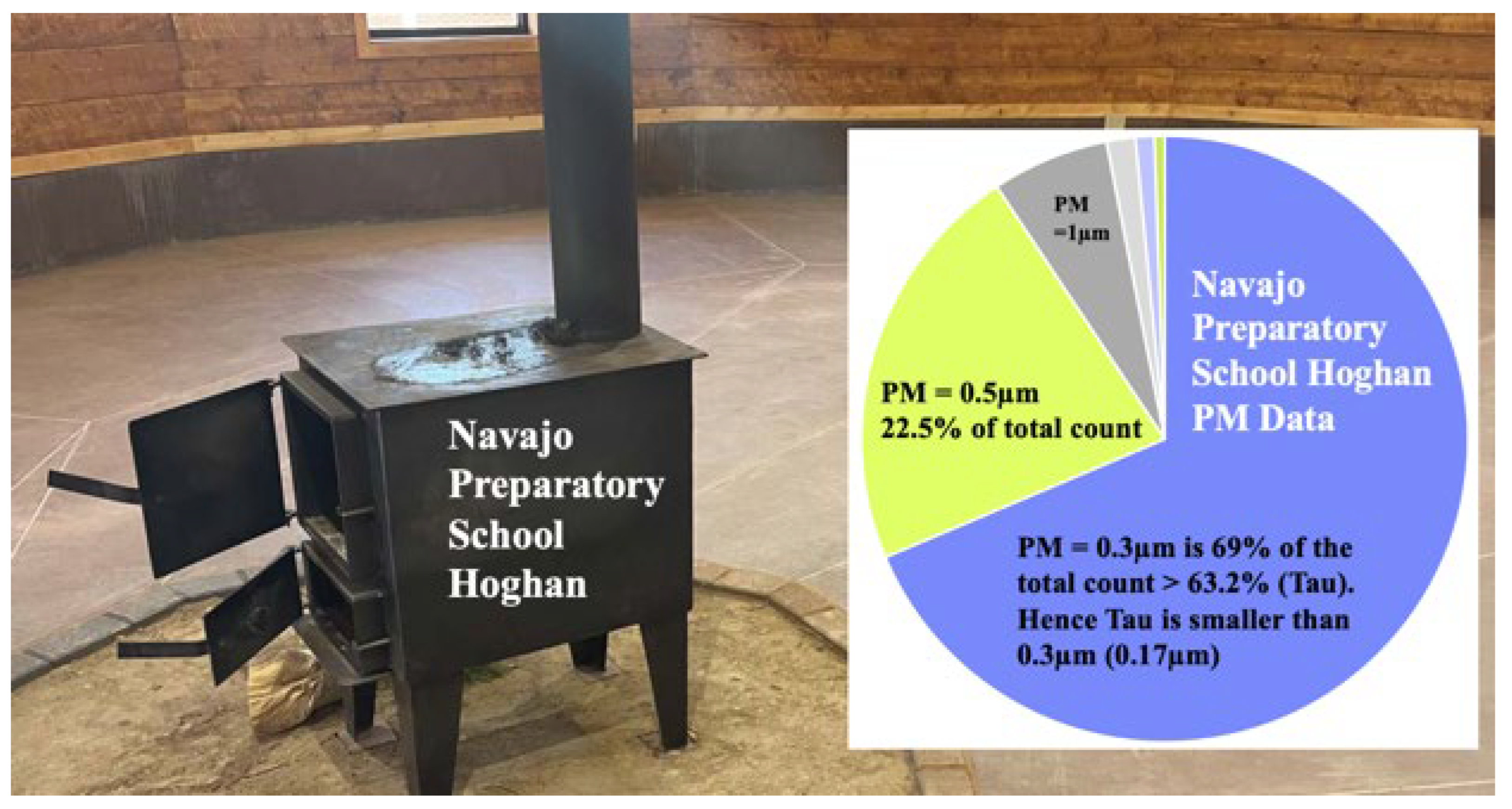
Table 3, 5, and 7. The units of Tau are µm (particle size) and Tau is smaller than the smallest measured particle of 0.3µm, in all cases. This can be explained via
Figure 11, which shows that the percentage of 0.3µm is 69% for the Navajo Hoghan, which exceeds the definition of Tau as the 63.2% percentile. Thus, Tau is understandably smaller than 0.3µm.
Assuming Gaussian Distributions for “Tau,” the average of “indoor Tau” in
Table 3 is 0.1675µm and the average of “outdoor Tau” in
Table 5 was 0.1711µm, such as calculated by the example Excel function =AVERAGE(B2:B10). The standard deviation of “indoor Tau” in
Table 3 is 0.0062µm and the standard deviation of “outdoor Tau” in
Table 5 was 0.0033µm, such as calculated by the example Excel function =STDEV.S(B2:B10). These parameters can be applied to the Standardized Normal Variate Test Statistic ”Z.” Assuming there was no difference between the average indoor Tau and the outdoor Tau, the following equation was used, [
11]:
TAU1 = average indoor Tau = 0.1675µm
TAU2 = average outdoor Tau = 0.1711µm
SD1 = standard deviation of indoor Tau = 0.0062µm,
SD2 = standard deviation of outdoor Tau = 0.0033µm
M1 = 12 indoor samples from
Table 3
M2 = 9 outdoor samples from
Table 5
The units of Test Value Z are µm/µm, which means that Z is unitless, as desired. The value of Z from the above information is Z = 1.711, which equates to α/2 = 5% [
12]. Given this is a two-tailed test, this gives α = 10%, or a 90% confidence that the indoor and outdoor values of Tau are statistically equal.
The next item which is of interest is that the “Amount A” can be much larger for
Table 3 (indoor measurements) than
Table 5 (outdoor measurements). The explanation is that indoor rooms can act as “dust accumulators.” This indicates that indoor rooms need to be kept clean for respiratory health. An example is the Bahe Dorm Room, with the lowest “Amount A” of all samples, which shows the importance of cleanliness and neatness. On the other hand, the carpeted Zah Living Room had a very high “Amount A” due to the dust accumulated in the carpeting.
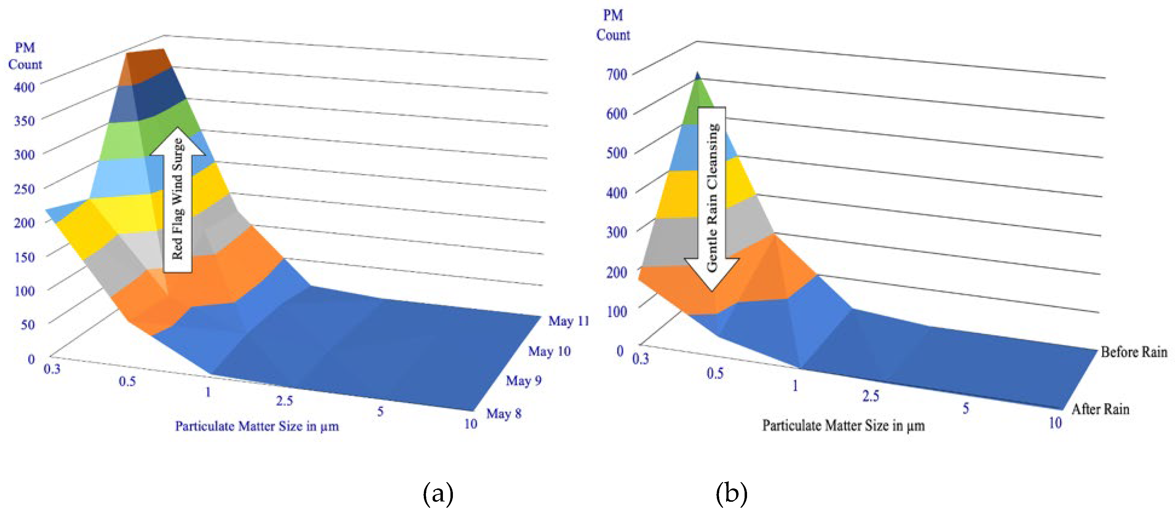
The final item of interest is shown in
Figure 12. The left graph shows how high velocity winds during a “red flag warning” clearly lift a lot of dust into the air. However, the right graph shows how a gentle rain cleanses particulate matter out of the outdoor air. The time axis in each graph in
Figure 12 is arranged to show the lower PM counts in the forefront, to keep the higher PM counts from obscuring the lower PM counts.
5. Conclusions
The Arduino DAS (Data Acquisition System) shown in
Figure 1 only cost
$77 (Arduino Uno
$27, PMSA003 Particulate Matter sensor
$52). Thus, a personal goal of a DAS for under
$100 was met.
The average particle counts shown in
Table 2 and
Table 4 were individually modeled by a negative exponential distribution, and this theoretical model had a correlation “R” of 99.08% - 99.99% with the experimental data, Tables 3, 5, and 7. This proved that it was possible to model the distribution of particulate matter sizes. Both the theoretical model and the experimental data showed that the 0.3 particle size was dominant, which makes sense. Assuming that the 10 and 0.3 micrometer particle sizes have the same mass density, the ratio of the masses of the two particles is a function of radius or diameter to the third power (the volume of a sphere). This mass ratio is (10/0.3)
3 which shows that the 10-micrometer particle has 37,000 times the mass of the 0.3-micrometer particle. Hence, the 10-micrometer “coarse” particles would tend to settle out more readily and the 0.3-micrometer “fine” particles would tend to stay airborne.
For all locations tested, that the “63.2% percentile” Tau varied between 0.15 and 0.18 micrometers, and that the indoors Tau was statistically equal to the outdoor Tau.
Figure 11 showed that the percentage of 0.3µm particulate matter 69% exceeded 63.2% (Tau) for the Hoghan, which explains why Tau was smaller than 0.3µm in Tables 2, 4, and 6.
Based on the above, our hypotheses were accepted, namely that we could create a data acquisition system for under $100, that we could program this DAS and use it to gather actual data, and that we could curve fit a theoretical model to the actual particulate matter data to an extremely high statistical correlation.
The importance of this research is that the “fine” particulate matter is highly mobile. Fine (0.3 um) radioactive dust, dust from farmers plowing their fields, and particulate matter from forest fires could remain in the air for a long time, thus causing the harmful effects documented by the U.S. Environmental Protection Agency. This is highly relevant to the Navajo Nation.
Follow-on research could include putting heat exchangers in the exhaust pipes of wood-burning stoves in Hoghans, so that less wood needs to be burned and hence less particulate matter and less carbon monoxide produced.
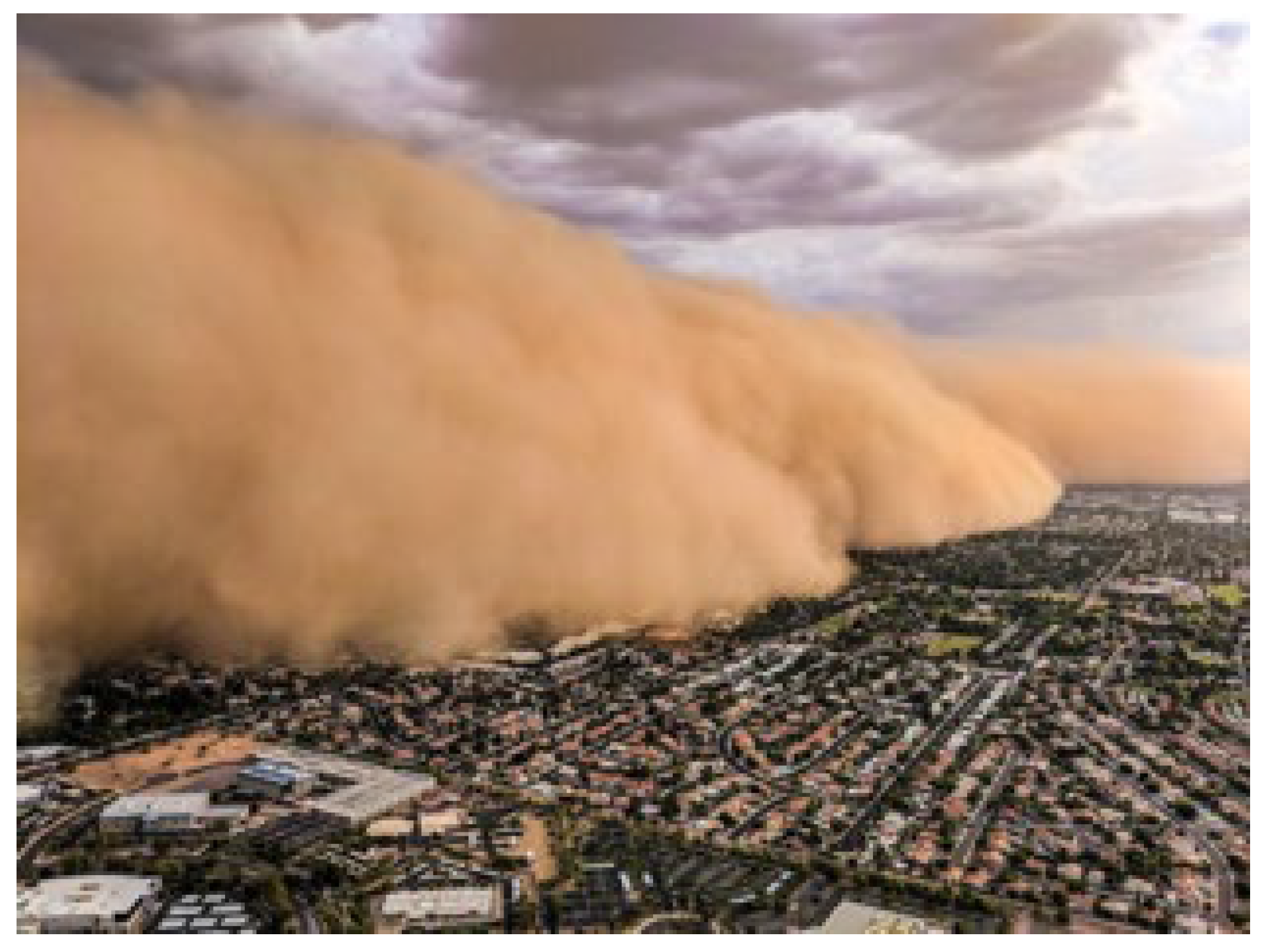
Our recommendations for dust control include the use of soil stabilizers on agricultural land, and dirt roads on the Navajo Nation, to prevent catastrophic dust storms,
Figure 13. Dust-launching leaf blowers would be taken off the market, and people would go back to using brooms. Within structures, such as the classrooms and dorm rooms at Navajo Preparatory School, frequent changes of the air filters in the air handling systems are recommended, as well as the use of Honeywell HPA300 HEPA (High-Efficiency Particulate Air) Air Purifiers in classrooms, [
13]. These HEPA filters remove 99.97% of particulate matter which are 0.3 micrometers or larger in size.
Figure 14, [
15], shows how devastating smoke particulate matter can be. This photo was taken of the Lower Manhattan, New York City. The source of the smoke particulate matter was the wildfires in Canada. As our global climate warms, harmful particulate matter will grow as a problem, which means we must act now to reverse climate warming.
Figure 1.
Arduino UNO tracking 0.3, 0.5, 1, 2.5, 5, 10 µm “PM” Particulate Matter.
Figure 1.
Arduino UNO tracking 0.3, 0.5, 1, 2.5, 5, 10 µm “PM” Particulate Matter.
Figure 2.
PMSA003 Particulate Matter Sensor counting 0.3, 0.5, 1, 2.5, 5, 10 µm “PM”.
Figure 2.
PMSA003 Particulate Matter Sensor counting 0.3, 0.5, 1, 2.5, 5, 10 µm “PM”.
Figure 3.
Map of the Navajo Nation [
5].
Figure 3.
Map of the Navajo Nation [
5].
Figure 4.
Abandoned Uranium Mines on and near the Navajo Nation [
6].
Figure 4.
Abandoned Uranium Mines on and near the Navajo Nation [
6].
Figure 5.
Flow Chart of Data Acquisition and Post-Processing.
Figure 5.
Flow Chart of Data Acquisition and Post-Processing.
Figure 6.
Actual Data Displayed on a Laptop from the Arduino UNO.
Figure 6.
Actual Data Displayed on a Laptop from the Arduino UNO.
Figure 7.
Graph of Particle Count vs Particle Size, Bahe Dorm Room, Navajo Preparatory School.
Figure 7.
Graph of Particle Count vs Particle Size, Bahe Dorm Room, Navajo Preparatory School.
Figure 8.
Negative Exponential Curve Fit vs Measured Particle Matter Count: Bahe Dorm Room.
Figure 8.
Negative Exponential Curve Fit vs Measured Particle Matter Count: Bahe Dorm Room.
Figure 9.
Particle Sizes versus Wavelengths of Light.
Figure 9.
Particle Sizes versus Wavelengths of Light.
Figure 10.
(a) Smoky Air in West Virginia worse than New Mexico and Arizona and (b) Sunlight in Smoky West
Virginia.
Figure 10.
(a) Smoky Air in West Virginia worse than New Mexico and Arizona and (b) Sunlight in Smoky West
Virginia.
Figure 11.
Pie Chart of Particle Count vs Size (Table 2), for Navajo Preparatory School Hoghan [10].
Figure 11.
Pie Chart of Particle Count vs Size (Table 2), for Navajo Preparatory School Hoghan [10].
Figure 12.
(a) Red Flag Winds Cause PM Surge, then (b) Gentle Rains Cleanse the Air.
Figure 12.
(a) Red Flag Winds Cause PM Surge, then (b) Gentle Rains Cleanse the Air.
Figure 13.
Catastrophic Dust Storm - Monsoon Outflow, August 20, 2018, Phoenix, Arizona [
14].
Figure 13.
Catastrophic Dust Storm - Monsoon Outflow, August 20, 2018, Phoenix, Arizona [
14].
Figure 14.
Catastrophic Wildfire Smoke in New York City from Canadian Fires, June 8, 2023 [
15].
Figure 14.
Catastrophic Wildfire Smoke in New York City from Canadian Fires, June 8, 2023 [
15].
Table 1.
Independent and Dependent Variables.
Table 1.
Independent and Dependent Variables.
| Independent Variables |
Dependent Variables |
| N = 6 different Particulate Matter sizes: 0.3, 0.5, 1, 2.5, 5, 10 µm |
Average, Maximum, and Minimum counts of each Particulate Matter size. |
| |
Least-Squares fit of “Amount A” and Tau (63.2% “percentile”) of negative exponential distribution of particulate matter “PM” count versus size in micrometers): .
Correlation “R” between Negative Exponential Distribution and actual measured PM counts.
Student t-Distribution Confidence: .
Standardized Test Statistic, Z. |
Table 2.
Average Particulate Count for N=6 Particle Sizes, 12 Indoor Sites.
Table 2.
Average Particulate Count for N=6 Particle Sizes, 12 Indoor Sites.
Indoor Navajo
Preparatory School
|
PM 0.3 |
PM 0.5 |
PM 1.0 |
PM 2.5 |
PM 5 |
PM 10 |
| Bahe Dorm Room |
94.33 |
28.46 |
1.54 |
0.46 |
0.46 |
0.35 |
| Zah Living Room |
3788.41 |
1148.08 |
132.73 |
15.37 |
4.43 |
1.8 |
| Wolfe’s Room |
121.50 |
40.17 |
19.83 |
7.50 |
1.00 |
1.00 |
| Recreation Room |
171.45 |
51.70 |
2.97 |
0 |
0 |
0 |
| Manliteo Room |
472.50 |
149.71 |
26.92 |
12.54 |
2.67 |
1.88 |
| Library |
906.47 |
291.02 |
83.04 |
20.33 |
13.22 |
7.18 |
| Hoghan |
907.26 |
291.30 |
82.76 |
20.26 |
13.26 |
7.22 |
| Cafeteria Heater |
805.12 |
242.09 |
11.79 |
1.81 |
0.77 |
0.30 |
| Chemistry Room |
876.27 |
262.82 |
29.82 |
0 |
0 |
0 |
| Dorm Living Room |
115.29 |
30.71 |
0.76 |
0.76 |
0.76 |
0.76 |
| Bates Living Room |
820.25 |
230.77 |
2.72 |
0.40 |
0.32 |
0.32 |
| Arthur Hall |
145.05 |
45.70 |
12.26 |
6.88 |
0.86 |
0.86 |
Table 3.
Constants A and Tau, Correlation R, Confidence for Navajo Preparatory School.
Table 3.
Constants A and Tau, Correlation R, Confidence for Navajo Preparatory School.
Indoor Navajo
Preparatory School
|
Constant “A”
Ae-(PM-0.3)/Tau
|
Constant “Tau”
Ae-(PM-0.3)/Tau
|
Statistical
Correlation “R”
|
99.95% Confidence
N-2 = 4 DOF
|
| Bahe Dorm Room |
94.33 |
0.17 µm |
99.99% |
197.01 > 8.61 |
| Zah Living Room |
3,788.41 |
0.16 µm |
99.97% |
85.25 > 8.61 |
| Wolfe’s Room |
121.50 |
0.17 µm |
99.08% |
14.68 > 8.61 |
| Recreation Room |
171.45 |
0.17 µm |
99.99% |
278.99 > 8.61 |
| Manliteo Room |
472.50 |
0.17 µm |
99.93% |
56.93 > 8.61 |
| Library |
906.47 |
0.17 µm |
99.81% |
32.07 > 8.61 |
| Hoghan |
907.26 |
0.17 µm |
99.81% |
32.28 > 8.61 |
| Cafeteria Heater |
805.12 |
0.17 µm |
99.99% |
229.80 > 8.61 |
| Chemistry Room |
876.27 |
0.17 µm |
99.97% |
95.55 > 8.61 |
| Dorm Living Room |
115.29 |
0.15 µm |
99.99% |
219.41 > 8.61 |
| Bates Living Room |
820.25 |
0.17 µm |
99.99% |
197.60 > 8.61 |
| Arthur Hall |
145.05 |
0.17 µm |
99.99% |
30.89 > 8.61 |
Table 4.
Average Particulate Count for N=6 Particle Sizes, 9 Outdoor 2023 Dates.
Table 4.
Average Particulate Count for N=6 Particle Sizes, 9 Outdoor 2023 Dates.
Tucson,
Arizona |
PM 0.3 |
PM 0.5 |
PM 1.0 |
PM 2.5 |
PM 5 |
PM 10 |
| May 8 |
218.82 |
67.76 |
4.57 |
0.57 |
0.57 |
0.57 |
| May 9 |
199.98 |
63.10 |
19.06 |
6.61 |
0.75 |
0.75 |
| May 10 red flag |
395.90 |
126.22 |
20.35 |
3.38 |
2.92 |
1.52 |
| May 11 |
378.97 |
121.16 |
8.94 |
0 |
0 |
0 |
| May 13 |
494.51 |
159.57 |
16.22 |
0.96 |
0.96 |
0.96 |
| May 14 |
355.18 |
109.51 |
9.20 |
0.63 |
0.43 |
0.43 |
| May 16 wind |
620.44 |
196.17 |
20.44 |
0.44 |
0 |
0 |
| May 19 5mm rain |
174.3 |
54.10 |
3.8 |
0 |
0 |
0 |
| May 20 |
292.36 |
107. |
8.27 |
0 |
0 |
0 |
Table 5.
Constants A and Tau, Correlation R, Confidence for Outdoor Tucson, Arizona.
Table 5.
Constants A and Tau, Correlation R, Confidence for Outdoor Tucson, Arizona.
Outdoor Tucson,
Arizona 2023
|
Constant “A”
Ae-(PM-0.3)/Tau
|
Constant “Tau”
Ae-(PM-0.3)/Tau
|
Statistical
Correlation “R”
|
99.95% Confidence
N-2 = 4 DOF
|
| May 8 |
218.82 |
0.17 µm |
99.99% |
130.44 > 8.61 |
| May 9 |
199.98 |
0.17 µm |
99.93% |
53.18 > 8.61 |
| May 10 red flag |
395.90 |
0.17 µm |
99.98% |
94.55 > 8.61 |
| May 11 |
378.97 |
0.17 µm |
99.98% |
94.15 > 8.61 |
| May 13 |
494.51 |
0.18 µm |
99.98% |
101.87 > 8.61 |
| May 14 |
355.18 |
0.17 µm |
99.98% |
127.16 > 8.61 |
| May 16 wind |
620.44 |
0.17 µm |
99.98% |
104.32 > 8.61 |
| May 19 5mm rain |
174.3 |
0.17 µm |
99.99% |
121.31 > 8.61 |
| May 20 |
292.36 |
0.17 µm |
99.99% |
125.50 > 8.61 |
Table 6.
Average Particulate Count for N=6 Particle Sizes, Smoky Air Data, West Virginia.
Table 6.
Average Particulate Count for N=6 Particle Sizes, Smoky Air Data, West Virginia.
West Virginia
29 June 2023
|
PM 0.3 |
PM 0.5 |
PM 1.0 |
PM 2.5 |
PM 5 |
PM 10 |
| Smoky indoor |
10672.2 |
3459.9 |
1120.0 |
108.1 |
21.5 |
7.0 |
| Smoky outdoor |
11490.3 |
3724.9 |
1222.9 |
123.9 |
25.4 |
8.9 |
| Outdoor+24 hours |
3581.8 |
1157.6 |
334.8 |
25.6 |
5.3 |
1.9 |
Table 7.
Constants A and Tau, Correlation R, Confidence for Smoky Air Data, West Virginia.
Table 7.
Constants A and Tau, Correlation R, Confidence for Smoky Air Data, West Virginia.
West Virginia
29 June 2023
|
Constant “A”
Ae-(PM-0.3)/Tau
|
Constant “Tau”
Ae-(PM-0.3)/Tau
|
Statistical
Correlation “R”
|
99.95% Confidence
N-2 = 4 DOF
|
| Smoky Indoor |
10672.2 |
0.18 µm |
99.97% |
80.62 > 8.61 |
| Smoky Outdoor |
11490.3 |
0.18 µm |
99.97% |
79.45 > 8.61 |
| Outdoor+24 hours |
3581.8 |
0.18 µm |
99.97% |
86.28 > 8.61 |