
Submitted:
20 January 2025
Posted:
20 January 2025
You are already at the latest version
Abstract
This study examines the impact of soil temperature on radon transport and exhalation near Sakurajima volcano, Japan. Continuous soil temperature measurements at various depths revealed a thermal gradient, with decreasing fluctuations at greater depths, leading to more stable radon emissions. This finding underscores the importance of accurate temperature data in understanding radon transport dynamics. The research highlights the influence of temperature on soil-gas permeability by affecting the dynamic viscosity of soil gases. Discrepancies between measured and calculated temperature profiles, using constant thermal diffusivity and mean surface temperature for all layers, suggest that these parameters are site-specific and cannot be generalized. This study offers valuable insights for optimizing radon monitoring programs by establishing the optimal depth placement for radon detectors of 80-100 cm and developing a framework for correcting radon measurements for temperature-induced variations. These advancements enhance the reliability and accuracy of radon as a precursor for geohazard studies and volcanic activity.
Keywords:
soil temperature profile
; modelling
; volcano activity
; geohazard
; thermal diffusivity
; thermal gradient
; radon
1. Introduction
The prediction of geohazards events such as volcanic eruptions and earthquakes represents a significant and challenging area of research within the wider context of Earth science, given the inherent complexities of the planet’s natural processes. Among various techniques such as low-frequency acoustic emission, mechanical deformations of the lithosphere, changes in the level and composition of groundwater, temperature fluctuations, propagation of acoustic gravity waves, fluctuations of electric and magnetic field components, ground-based observations of ionospheric parameters, the study of radon gas has emerged as one of the valuable approaches [1]. Observing changes in radon concentration in soil, water and atmosphere allows us to obtain subtle but valuable information on geological activity, especially in terms of identifying anomalies caused by the movement of the Earth’s crust. As concluded by Woith, who analysed over 100 scientific papers, the following points were highlighted: (i) significant radon anomalies exist; (ii) seismo-tectonically induced radon anomalies likely occur; and (iii) radon anomalies of non-tectonic origin can exist and may appear strikingly like tectonic ones. Consequently, it is presumed that only a fraction of reported radon precursors is genuinely related to the physical processes associated with the preparation of impending earthquakes. While radon is a powerful tracer for fluid movements and pressure transients in the Earth’s crust, distinguishing between external (e.g., meteorological or anthropogenic) signals and seismo-tectonic ones remains a critical challenge [2].
In order to ascertain the relationship between volcanic activity and radon, while minimising the influence of meteorological factors, comprehensive measurements have been initiated in the vicinity of Sakurajima, is the most active volcano in Japan according to the Japan Metrological Agency [3]. The monitoring programme includes the measurement of radon exhalation rate and a range of climatic parameters, including outdoor temperature, atmospheric pressure, wind speed and direction, and precipitation. To eliminate the influence of environmental parameters on radon signalling anomalies, it is essential that knowledge of other parameters such as soil temperature and soil moisture are available, which are also recorded as part of the monitoring programme. Therefore, understanding the interplay of temperature, soil permeability, and dynamic viscosity represents a key area of research to facilitate the forecasting of these natural phenomena.
Soil temperature is crucial for determining the dynamic viscosity of soil, which affects soil-gas permeability as described by the modified Darcy equation [4]: , where k is soil-gas permeability (), q is volumetric flux (), is the pressure gradient (Pa), F is the soil probe shape factor (m), and is the dynamic viscosity of the gas (Pa·s), dependent on gas type and temperature.
The dynamic viscosity can be assessed by the Arrhenius-like equation: , where: is the viscosity at a reference condition and acts as a baseline for comparing how viscosity changes with temperature, is an activation energy (J ), R is the universal gas constant of 8.3145 (J ), and T is an absolute temperature (K).
In processes like diffusion, represents the energy needed for particles (atoms, ions, or molecules) to overcome barriers such as lattice vibrations or inter-particle attractions. In soil systems, often corresponds to the viscosity of water or a soil-water mixture at the reference temperature. For soil-water mixtures, depends on the soil composition, particle size distribution, and salinity of the pore water.
As mentioned earlier, accurate temperature data is essential for understanding subsurface processes and identifying potential radon anomalies. However, the presence of missing data can complicate further analysis and obscure critical insights. To address this, it is important to implement robust data collection and validation techniques. The identification and rectification of probe failures or data anomalies is of crucial importance in ensuring the reliability of temperature measurements.
There are two main objectives of this work:
- To analyse and characterize long-term soil temperature profiles at different depths (ambient, 10 cm, 40 cm, and 100 cm) near an active volcanic region, including their seasonal variations and thermal gradients,
- To develop and validate mathematical models for predicting soil temperature variations with depth, with specific focus on improving radon transport monitoring in volcanic regions.
The collection of detailed soil and meteorological parameters presented in this paper ensured the creation of a robust dataset for the analysis of environmental factors affecting radon transport and release dynamics. However, the present study focused exclusively on temperature variability, without undertaking further analysis or correlation with other environmental parameters.
2. Materials and Methods
2.1. Measurement Site
Sakurajima, located in Kagoshima Prefecture, is widely acknowledged as the most active volcano in Japan, thus rendering it a pivotal locale for volcanological research.The Minamidake crater, situated at the summit of Sakurajima, has been undergoing near-continuous explosive eruptions since 1955, while activity at the Showa crater resurfaced in 2006, resulting in nearly daily explosive eruptions. This persistent activity, in combination with the volcano’s intricate geological composition, engenders a distinctive environment conducive to the study of radon exhalation from the ground and its correlation with volcanic processes [5].
For the purposes of this study, measurements were conducted at a site in Tarumizu City, located approximately 10 kilometres southeast of the Minamidake crater. The selected site is positioned within an area characterised by hypersthene rhyolite ash and sand deposits, as documented by the Geological Survey of Japan [6]. The geology of the region exerts a substantial influence on radon transport and exhalation rates, which are pivotal parameters for comprehending the interplay between radon exhalation and volcanic activity. The implementation of continuous monitoring at the site in question facilitates the acquisition of high-resolution radon data, which can subsequently be correlated with seismic and eruption events at Sakurajima. This, in turn, serves to enhance our understanding of the precursory signs of volcanic activity.
2.2. Measurement Method
Soil temperature profiles were continuously recorded at three depths (10 cm, 40 cm, and 100 cm below the surface) using a TEMPPRO device. Concurrently, meteorological parameters, encompassing atmospheric temperature, pressure, relative humidity, quantum light, solar radiation, wind speed, and wind direction, were systematically monitored using a meteorological station (WatchDog 2900 ET, Spectrum Technology Inc., USA) installed at the measurement site. Atmospheric concentrations were measured at the same location. Rainfall data were sourced from the meteorological post at Tarumizu City Hall to complement the onsite measurements. Additionally, the volumetric water content of the soil was measured across six layers spanning depths from 10 cm to 100 cm. All data were collected in 1-hour cycles.
2.3. Numerical Modelling
The ambient temperature can be modelled using a sinusoidal function, expressed by the following equation:
where: is the average (or baseline) temperature (oC), A is the amplitude, representing the temperature variation around the average (oC), t is the elapsed time (h), is the phase shift, indicating when the sinusoidal curve starts (h), is the angular frequency (rad ), calculated as , where T is the period (total time for one complete cycle); in this case the annual temperature cycle, i.e., T = 365 * 24 = 8760 h.
The vertical temperature distribution of the ground was modelled using the refined approach described by Florides and Kalogirou [7,8], based on the model developed by Kasuda and Achenbach [9]. Their model determines ground temperature as a function of time and depth below the surface, described by:
where: is the soil-air temperature at depth Z and time t ( ∘C), is the mean ambient temperature ( ∘C), is the surface temperature amplitude, calculated as (C), Z is depth (m), is the time from the start of the year to minimum temperature occurrence (h), is thermal diffusivity ()
The relationship between minimum temperature time (), maximum temperature time (), and phase shift () is given by the relatioships: and .
3. Results and Data Analysis
Figure 1 presents the observed ambient temperature collected at the height of 100 cm above the ground and temperature profiles at depths of 10 cm, 40 cm, and 100 cm over a 9-year period from 2015-07-24 to 2024-10-25. However, the data set is incomplete due to technical difficulties such as power outages or equipment malfunctions.
A clear thermal gradient is evident, with temperature lines at different depths exhibiting noticeable fluctuations. The temperature range at a depth of 100 cm is significantly smaller compared to the shallower depths of 10 cm and 40 cm. This finding indicates potential variations in the soil’s thermal properties, with deeper layers exhibiting enhanced stability. Both ambient and soil temperatures demonstrate clear seasonal variations, with the amplitude of temperature fluctuations diminishing with increasing depth. At the ambient level as well as at depths of 10 cm and 40 cm, temperature fluctuations between summer and winter are more pronounced. Conversely, the 100-cm depth exhibits a more stable temperature throughout the year, suggesting that deeper soil layers are less influenced by surface temperature variations. As previously indicated, the development of a model capable of predicting soil temperature based on measurements of outdoor temperature will facilitate more precise and efficacious data analysis, particularly in cases where radon transport or permeability are being investigated or for statistical analysis like trend and harmonic.
3.1. Data Analysis
The results of long-term measurements of ambient and profile soil temperature are summarized in Table 1.
An analysis of the temperature data revealed vertical thermal variations across four distinct levels. The ambient and shallow depth (10 cm) levels exhibited the most significant temperature range, with fluctuations ranging from -C to C. In contrast, deeper soil layers demonstrated a reduction in temperature variability. At a depth of 100 cm, temperatures stabilised within the range of C and C. The median temperatures were found to be consistent across the profile, ranging from C to C, with a peak recorded at 10 cm. The SD indicated variability within each level, with the highest SD observed at ambient and 10 cm depths (both C), and the lowest SD recorded at 100 cm depth (C), reflecting more stable temperatures at greater depths.
All depths exhibited slight negative skewness, with values ranging from −0.12 to −0.35, indicating distributions marginally shifted towards higher values. The kurtosis values were consistently negative across all depths, ranging from −0.71 to −1.50, indicating flatter, more spread-out distributions with fewer extreme values than would be expected in a normal distribution. The most pronounced uniform distribution was observed at Z = 100 cm (kurtosis = −1.50).
3.2. Modelling
The temperature oscillations were modelled using Equations (1) and (2), with average values taken from the 9-year measurement period for different depths and ambient conditions. The results presented in Table 2 summarizes the fitted values of thermal diffusivity (), and peak temperature times (, ).
Observed and modelled temperature data are compared in Figure 2, with the corresponding fit parameters presented in Table 2.
As shown, the observed ambient and 10 cm depth temperatures exhibit higher frequency fluctuations and generally higher peak values compared to deeper measurements. While the model captures the overall seasonal trend, it underestimates temperature fluctuations, particularly at the surface (10 cm). As depth increases, the agreement between calculated and observed temperatures improves, with the curves aligning more closely at 40 cm and 100 cm. This suggests that the model performs better at greater depths, where temperature variations are more stable, confirming the phenomenon of thermal buffering.
The observed increase in soil thermal diffusivity () and the phase parameter of sinusoidal temperature oscillation () with depth, as presented in Table 2 and Figure 3, reflects the combined effects of soil composition, structure, and moisture content.
The relationship between and depth (Z) follows an exponential decay curve, i.e., . The phase parameter increases from about 2900 to 3500 hours, indicating that deeper soil layers take longer to reach their minimum and maximum values than shallower layers (Figure 3A). This delay with depth can be attributed to the insulating properties of the soil.
Moreover, the relationship between thermal diffusivity () and depth (Z) is found to be exponential, i.e. , which means an increase from almost zero at the surface to about 7 × at a depth of 100 cm (see Figure 4B).
At shallow depths, reduced thermal diffusivity is attributed to increased porosity, organic matter content, and the presence of air-filled pores, which serve to reduce thermal conductivity. At greater depths, soil compaction, increased bulk density, enhanced particle-to-particle contact, and stabilised moisture content improve thermal conductivity, while decreasing organic matter and reduced temperature fluctuations further contribute to higher thermal diffusivity. These findings emphasise the pivotal role of depth-dependent soil properties in modifying and delaying temperature variations, which has substantial implications for ground temperature modelling. The gradient in thermal diffusivity affects heat and mass transfer processes, including the transport of soil gases such as radon, influencing temperature-driven convective flows and diffusion rates within the soil matrix.
Figure 4 illustrates the modelled temperature variations at varying soil depths (10 cm, 40 cm, and 100 cm) and ambient conditions over the course of a year with the initial parameters of and from Table 2.
The temperature curves demonstrate a sinusoidal pattern indicative of annual temperature cycles, with temperatures ranging from approximately C to C. The amplitude of temperature variation exhibits a decrease with depth.
A critical aspect of the graph is the time shift in minimum and maximum temperatures at varying depths. The analysis reveals that minimum temperatures progressively lag with increasing depth relative to the ambient minimal temperature observed at the end of January (≈ 683 hours of the year ∼ 28 days). The delay is 88 h (≈3.5 days ∼end of January) at a depth of 10 cm, 311 hours at 40 cm (≈13 days ∼middle of February), and 681 h at 100 cm (≈28 days ∼end of February). A similar trend is observed for maximum temperatures, which also exhibit a lag with depth in relation to the maximum of ambient temperature at 5064 hours of the year (≈end of July). The delay is 79 h at 10 cm (≈3.3 days ∼begining of August), 310 h at 40 cm (≈13 days ∼middle of August) and 680 h at 100 cm (≈28 days ∼end of August). This phenomenon can be attributed to the principles of heat diffusion and the soil’s buffering effect on temperature fluctuations, which cause a delay and attenuation of temperature signals as they propagate through the soil medium, with each successive layer contributing to the cumulative delay.
Figure 5 compares modelled and observed soil temperature data, where each hour of the day represents the mean value for that specific hour calculated over the 9-year measurement period. Data were modelled using Equation (2) with input parameters as literature values of for volcanic soil [11,12] and a as the observed minimum ambient temperature.
The observed temperatures exhibit higher frequency fluctuations and generally higher peak values, particularly at the shallow depth of 10 cm. The model’s predictions effectively capture the overall seasonal trends but tend to underestimate temperature variations, especially near the surface. The agreement of oscillation between modelled and observed temperatures improves with increasing depth, indicating enhanced model performance in more thermally stable, deeper soil layers. However, a notable discrepancy exists between the measured and modelled temperatures (using constant and for all layers) for deeper layers, particularly regarding the time difference in the occurrence of minimum and maximum temperature values. This observation suggests that literature values of thermal diffusivity cannot be generalized and should account for specific soil properties and depth-dependent variations. The findings underscore both the necessity for precise temperature measurements to facilitate a comprehensive understanding of radon transport processes and the intricate nature of temperature dynamics across soil layers, particularly highlighting the challenges associated with accurately modeling near-surface temperature variations.
Figure 6 illustrates the seasonal variation of soil temperature profiles for both modelled and observed data with all layers (ambient and depth) for the average value of the entire period. The temperature profiles show clear seasonal stratification, with temperatures ranging from approximately 10 °C to 27 °C for the modelled data and from 11 °C to 32 °C for the observed data. Winter exhibits the coolest temperatures, while summer shows the warmest, with spring and autumn representing transitional periods. These findings reveal a distinct thermal gradient, demonstrating increasing thermal buffering with soil depth, which can be linked to an increase in thermal diffusivity.
However, the comparison reveals significant differences between observed and modelled soil temperatures at 10 cm depth across all seasons. These discrepancies are most pronounced in the transition seasons (spring and autumn), where the modelled temperatures consistently deviate from the observed values. This disparity may be attributable to either the influence of surface ambient conditions or potential sensor malfunctions.
The temperature profiles reveal interesting pattern similarities between winter-autumn and summer-spring pairs, demonstrating seasonal coupling in soil temperature dynamics (seasonal coupling refers to the synchronized patterns of change in soil temperature across different depths over the course of a year, driven primarily by seasonal variations in surface heat fluxes influenced by factors like solar radiation, air temperature, and precipitation).
In the winter-autumn pair, both seasons show that the temperature increases with depth, being lowest at ground level. In the spring-summer pair, the temperature decreases with depth. Therefore, the largest temperature range is observed at 0 cm and the smallest at 100 cm. At 10 cm and 40 cm depths, the temperature ranges are comparable; however, in the spring-autumn pair, the difference increases with depth.
These seasonal couplings likely reflect the transition periods in annual soil temperature cycles, where winter-autumn represents the cooling phase and summer-spring the warming phase of the soil profile. The similarity in patterns despite different absolute temperatures indicates the consistent nature of heat transfer processes during these paired seasons, though the model captures these dynamics with varying degrees of accuracy across different depths.
Using the data presented in Table 2, the modelling procedure was carried out and the results were then compared with the observed data throughout the entire measurement period (see Figure 7).
At the ambient level, the observed temperatures show significant variability, with clear seasonal oscillations ranging from −6 °C to 40 °C. The model data show comparable seasonal patterns, but with reduced short term variability and a more idealised sinusoidal curve in the range of 10 °C to 30 °C. The model data demonstrate comparable seasonal patterns, yet exhibit decreased short-term fluctuations, thus manifesting a more idealised sinusoidal curve. Moving deeper into the soil profile, at depths of 10 cm, 40 cm, and 100 cm, several key patterns emerge. Initially, at a depth of 10 cm, the model initially underestimates the observed temperatures. While the modelled data closely match the observations during the first years of measurement, they show increasing divergence in subsequent years. This progressive deviation could be attributed to either changing environmental factors or gradual sensor deterioration. Secondly, the amplitude of the temperature fluctuations gradually decreases with depth, suggesting a dampening effect of the soil environment. At a depth of 100 cm, the temperature fluctuations are significantly less pronounced compared to the ambient measurements. Thirdly, a substantial enhancement in the congruence between observed and modelled temperatures and depth is evident. The temporal resolution of the data appears to be quite high, capturing both diurnal and seasonal temperature fluctuations. The seasonal pattern demonstrates consistent annual cycles, with peaks occurring in the summer months and troughs in the winter. This cyclical pattern remains evident at all depths, although its magnitude decreases with increasing depth. This visualisation effectively demonstrates the ability of the soil to buffer temperature fluctuations, with deeper layers showing increased thermal stability and more predictable temperature patterns that are more in line with model expectations.
3.3. Model Sensitivity
The temperature model results can be used to evaluate implications for permeability calculations. Traditionally, permeability calculations have relied on air suction measurements at depths of 50–100 cm, while temperature measurements have typically been taken at shallower depths. The developed model can estimate soil temperatures at greater depths based on ambient temperature, thereby reducing the impact of temperature variations within the soil profile. For example, in summer, the temperature difference between 10 cm depth (where measurements are commonly taken) and 100 cm depth can reach approximately 10 °C. This temperature differential results in an approximate 11% variation in the calculated permeability k between these depths. These variations contribute significantly to the overall uncertainty in Geogenic Radon Potential (GRP) assessments [4].
4. Conclusions
In conclusion, this study presents a comprehensive framework for analyzing soil temperature profiles and their influence on radon transport and exhalation. The vertical temperature distribution is particularly significant, as the data reveals soil’s role as a thermal buffer, with temperature variations becoming less pronounced at greater depths. This buffering effect is evidenced by the notable lag in temperature changes compared to ambient conditions, particularly at 100 cm depth, where radon transport processes are less sensitive to seasonal temperature fluctuations. This observation is crucial for modeling radon fluxes, as the deeper, more thermally stable soil layers may provide a more consistent baseline contribution to overall ground-level radon emissions.
It should be noted that at 10 cm depth, significant discrepancies between modeled and observed data were identified, potentially indicating sensor malfunctions or the influence of local soil conditions, such as rapid changes in soil moisture. These findings emphasize the importance of robust data collection and validation techniques for accurate analysis.
The insights gained from this study are critical for enhancing geohazard monitoring programs, enabling a deeper understanding of the interplay between soil temperature, permeability, and radon transport. Future work will focus on investigating the influence of other environmental parameters on both temperature and radon transport dynamics.
Author Contributions
Conceptualization, M.H., S.T., M.J.; methodology, M.H.; formal analysis, M.J.; investigation, M.H., S.T., Y.O., N.A.; writing—original draft preparation, M.J.; writing—review and editing, M.H., S.T., Y.O., N.A.; visualization, M.J.; project administration, S.T.; funding acquisition, M.H., S.T., Y.O., N.A. All authors have read and agreed to the published version of the manuscript.
Funding
This study was partially funded by the Environmental Radioactivity Network Center (ERAN) Grant number: P-24-43, the Japan Society for the Promotion of Science (JSPS) KAKENHI Grant No. JP22H03010 and the "Project on Human Resource Development in Radiation Medicine for Responding to Complex Disasters (Theme 1: Dynamics of radioactive substances and air pollutants in the environment associated with earthquakes and volcanic activities and assessment of exposure and doses)".
Institutional Review Board Statement
Not applicable.
Informed Consent Statement
Not applicable.
Data Availability Statement
The datasets analysed in this study are available from the authors upon reasonable request, in accordance with the data sharing policies of QST and Hirosaki University. Data access may require a data sharing agreement.
Conflicts of Interest
The authors declare no conflicts of interest.
References
- Conti, L.; Picozza, P.; Sotgiu, A. A Critical Review of Ground Based Observations of Earthquake Precursors. Frontiers in Earth Science 2021, 9, 1–30. [Google Scholar] [CrossRef]
- Woith, H. Radon earthquake precursor: A short review. European Physical Journal: Special Topics 2015, 224, 611–627. [Google Scholar] [CrossRef]
- Japan Meteorological Agency and Volcanological Society of Japan. National catalogue of the active volcanoes in Japan (the fourth edition, English version), 2018.
- Janik, M.; Gomez, C.; Kodaira, S.; Grzadziel, D. Development of a New Tool to Simultaneously Measure Soil Permeability and CO2 Concentration as Important Parameters for Geogenic Radon Potential Assessment "Development of a New Tool to Simultaneously Measure Soil Permeability and CO 2 Concentration as Im 2024. [CrossRef]
- Hosoda, M.; Tokonami, S.; Suzuki, T.; Janik, M. Machine learning as a tool for analysing the impact of environmental parameters on the radon exhalation rate from soil. Radiation Measurements 2020, 138, 106402. [Google Scholar] [CrossRef]
- Geological Survey of Japan AIST. Geological Survey of Japan AIST, 2019. Geological map of Japan, 1:200 000, Kagoshima., 2019.
- Florides, G.; Kalogirou, S. Annual ground temperature measurements at various depths. 8th REHVA World Congress, Clima 2005, pp. 1–6.
- Florides, G.; Kalogirou, S. Measurements of Ground Temperature at Various Depths. Bridge Maintenance, Safety, Management, Resilience and Sustainability - Proceedings of the Sixth International Conference on Bridge Maintenance, Safety and Management 2012, pp. 399–406. [CrossRef]
- Kasuda, T.; Achenbach, P. Earth Temperature and Thermal Diffusivity at Selected Stations in the United States. Technical Report NBS REPORT 8972, 1965.
- Boukhriss, M.; Zhani, K.; Ghribi, R. Study of thermophysical properties of a solar desalination system using solar energy. Desalination and Water Treatment 2013, 51, 1290–1295. [Google Scholar] [CrossRef]
- Kasubuchi, T. The effect of soil moisture on thermal properties in some typical Japanese upland soils. Soil Science and Plant Nutrition 1975, 21, 107–112. [Google Scholar] [CrossRef]
- Suzuki, S.; Iiduka, K.; Sanada, A.; Ito, H.; Watanabe, F. Effects of thermal conductivity and diffusivity of a volcanic ash soil in central Ethiopian Rift Valley on soil temperatures. Journal of Arid Land Studies 2019, 101, 91–101. [Google Scholar]
Figure 1.
Observed temperatures at each measurement depth. Dashed lines and shadow boxes represent the mean temperature at each depth and ambient conditions, with a range of ±2 standard deviations (SD). In this study, a range of ±2 SD from the mean was used to identify potential outliers, as it encompasses approximately 95.4% of the data in a normal distribution, providing a robust balance between sensitivity to anomalies and minimizing the misclassification of natural variability.
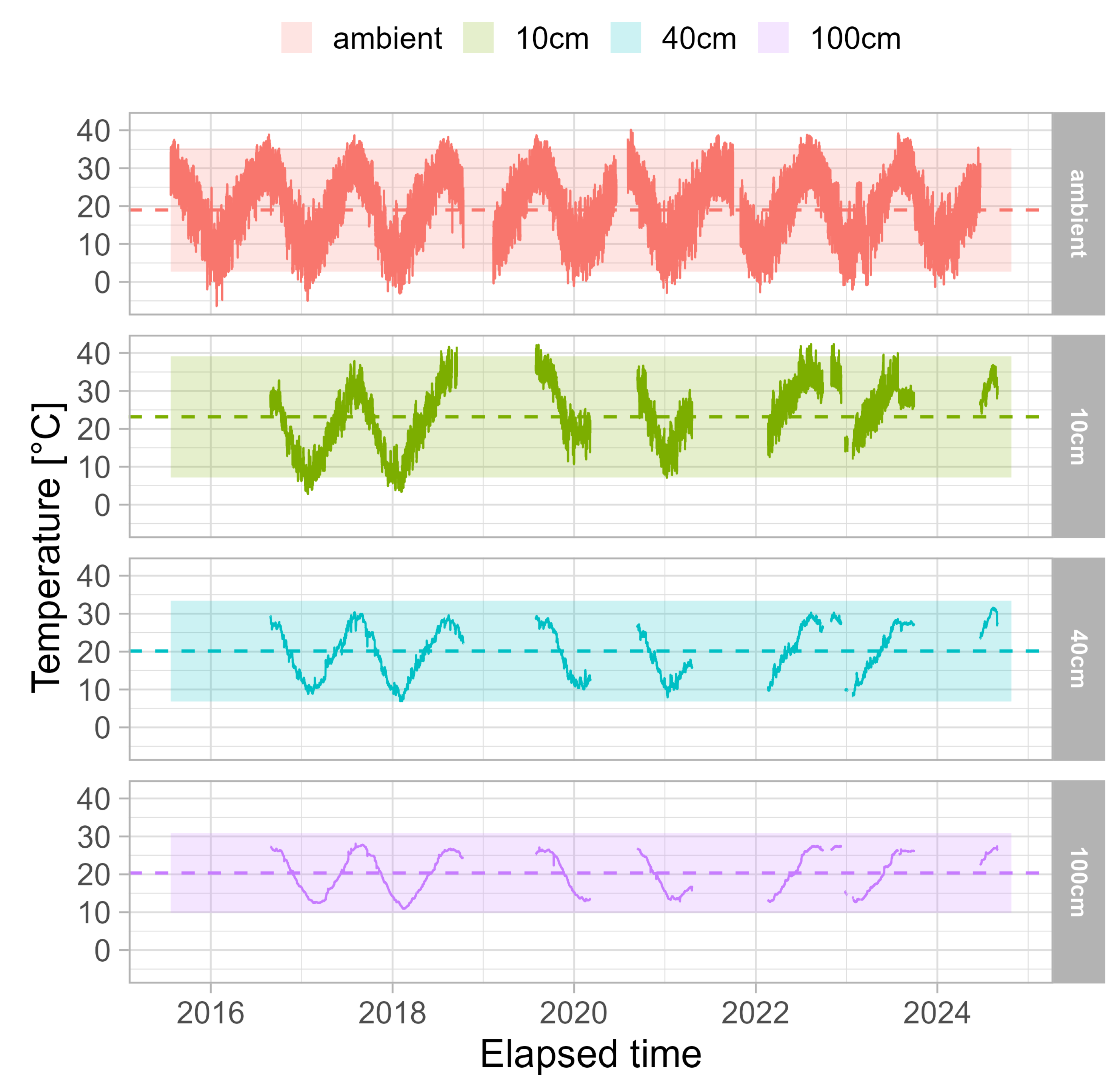
Figure 2.
Observed and modelled temperatures variations.
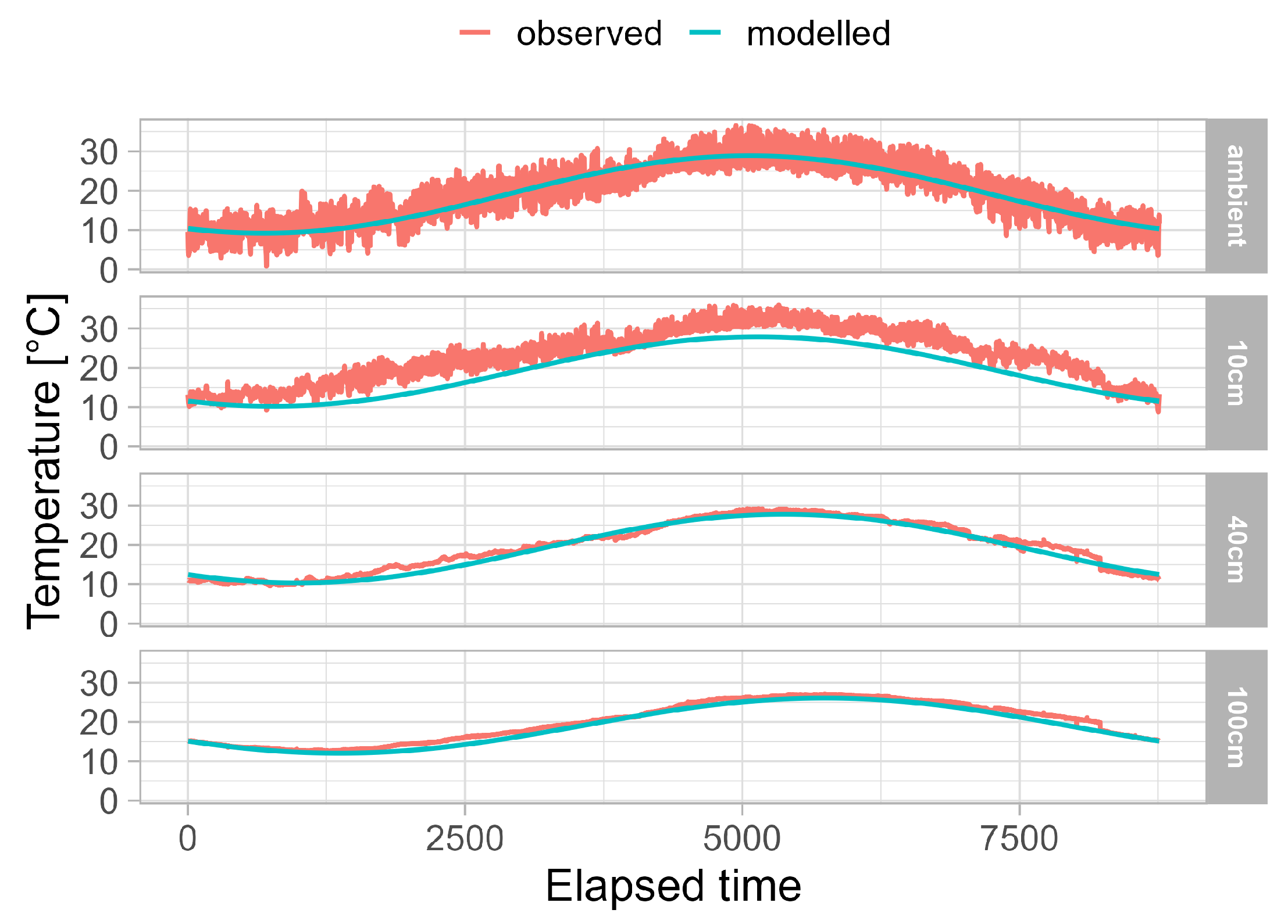
Figure 3.
Modelled thermal diffusivity () and tphase vs depth.
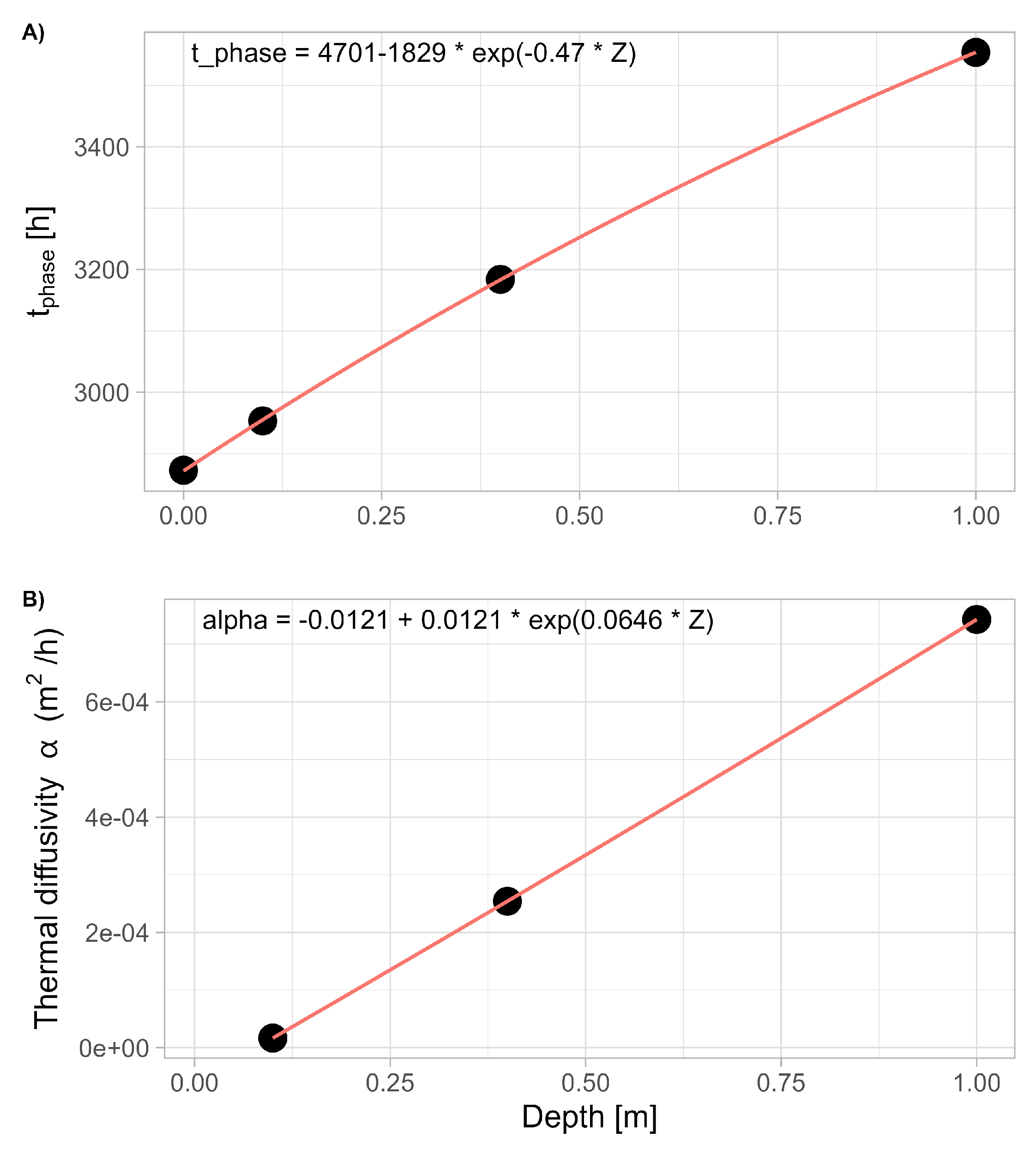
Figure 4.
Modelled temperature variations at different soil depths (10 cm, 40 cm, and 100 cm) and ambient conditions over a year, based on hourly averages from an 9-year measurement period with indication of and parameters.
Figure 4.
Modelled temperature variations at different soil depths (10 cm, 40 cm, and 100 cm) and ambient conditions over a year, based on hourly averages from an 9-year measurement period with indication of and parameters.
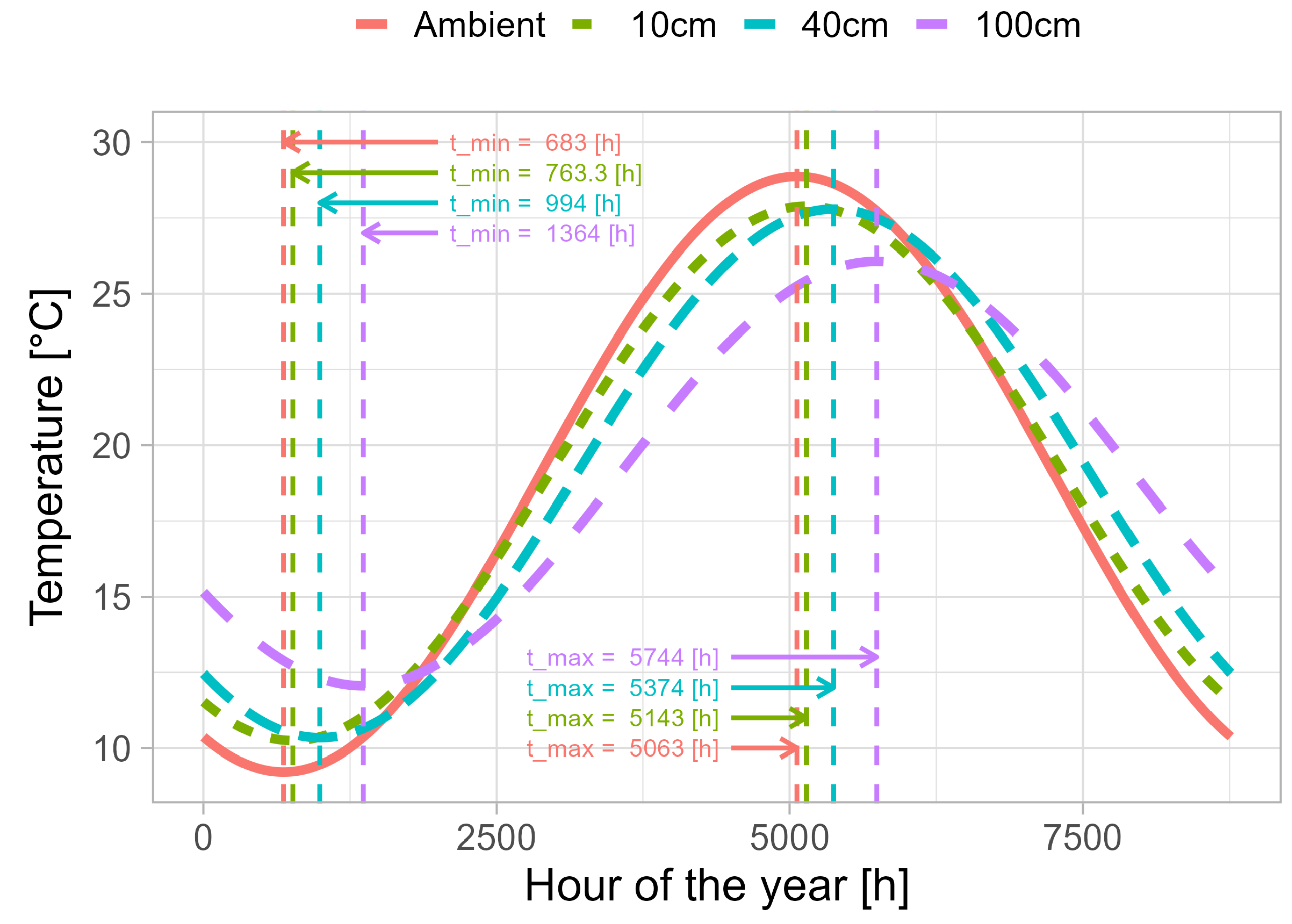
Figure 5.
Comparison of observed and modeled soil temperature data with constant and parameters.
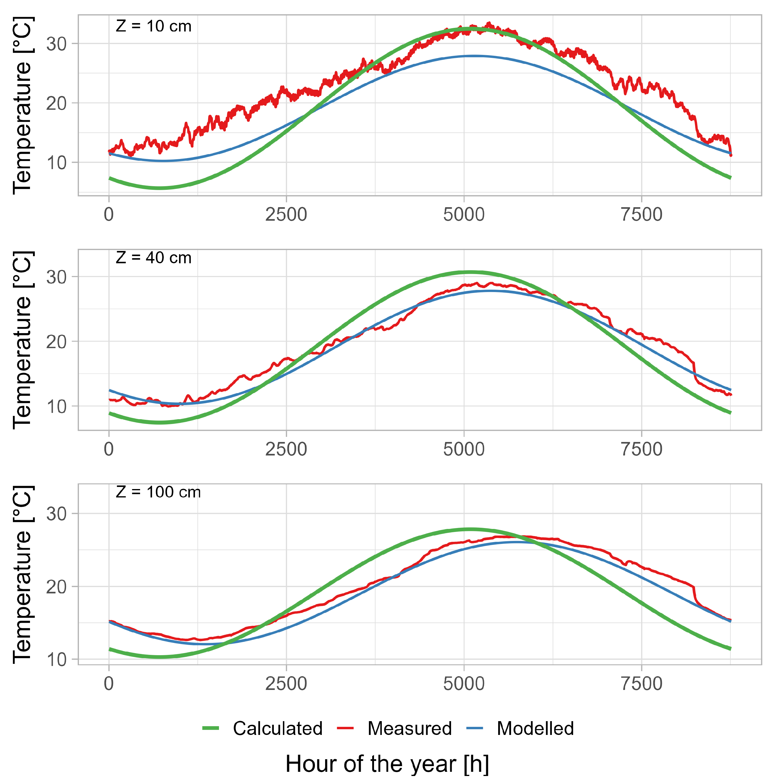
Figure 6.
Temperature variations across depth profiles for a continuous time span over mean value for different seasons (depth at 0 cm corresponds to ambient temperature measured at 100 cm above ground) for modelled (solid line) and observed (dashed line) data.
Figure 6.
Temperature variations across depth profiles for a continuous time span over mean value for different seasons (depth at 0 cm corresponds to ambient temperature measured at 100 cm above ground) for modelled (solid line) and observed (dashed line) data.
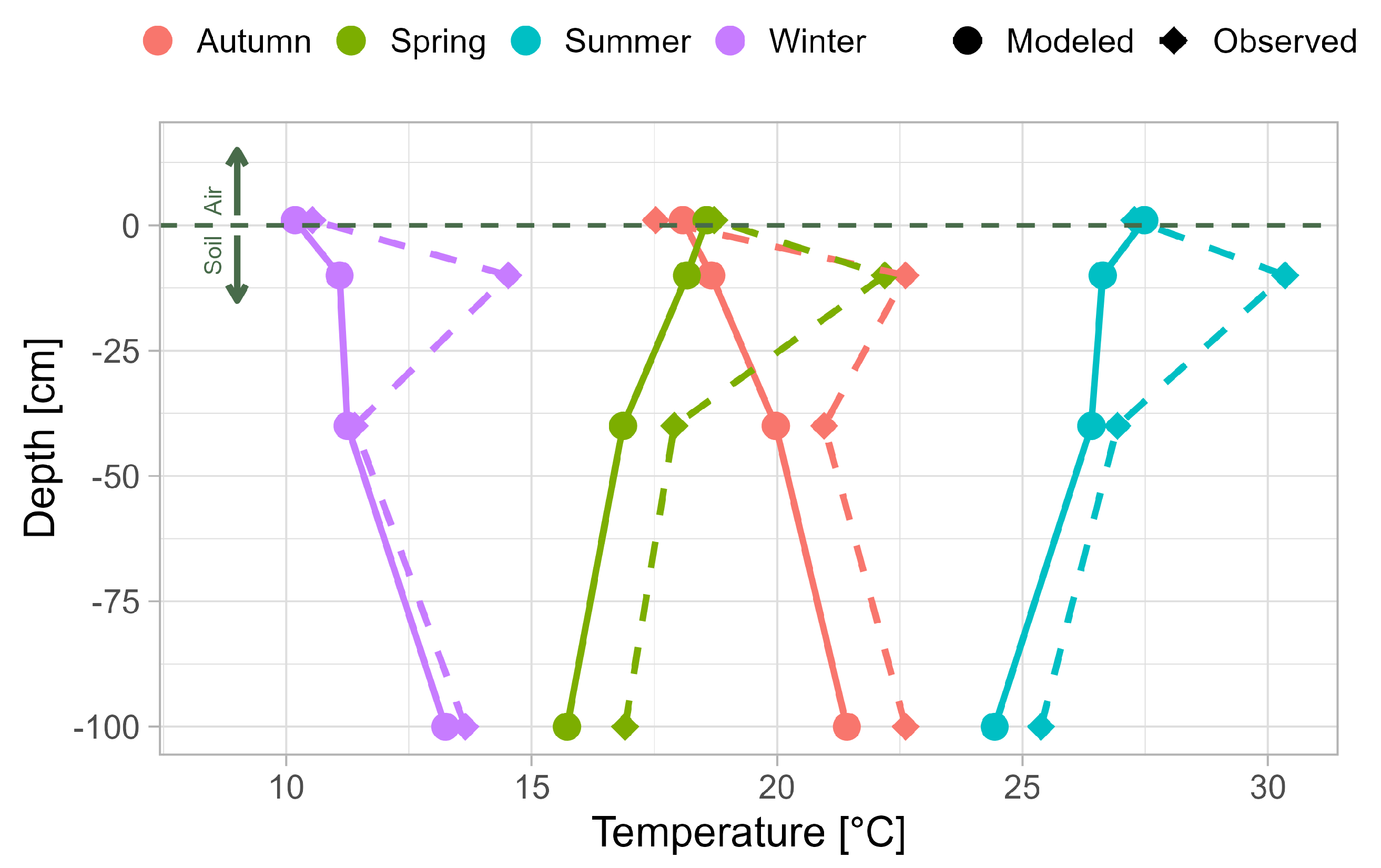
Figure 7.
Model application to whole observed data.
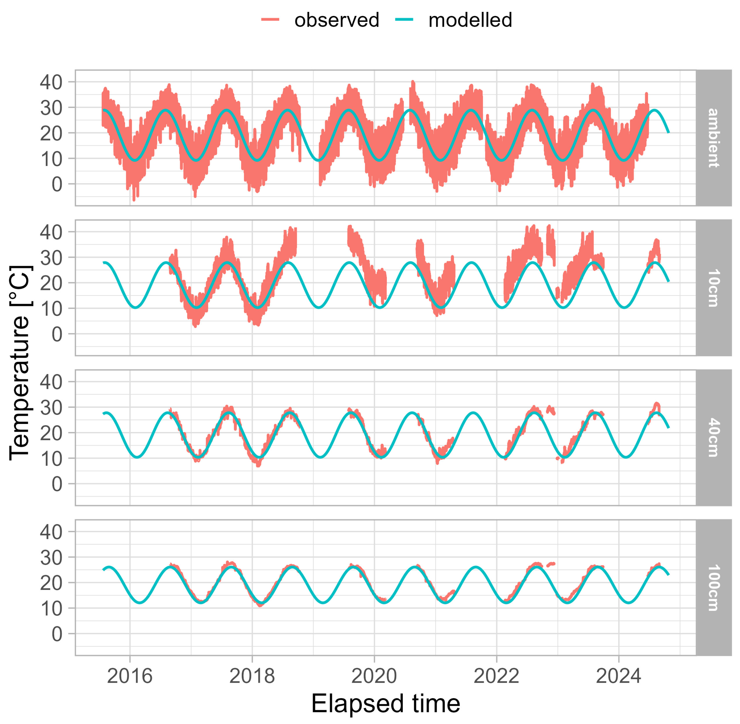

Table 1.
Summary statistics with minimum (Min) and maximum (Max) values, median (Med), mean (Mean), standard deviation (SD), Range, Skewness and Kurtosis according to each layer.
Table 1.
Summary statistics with minimum (Min) and maximum (Max) values, median (Med), mean (Mean), standard deviation (SD), Range, Skewness and Kurtosis according to each layer.
| Parameter | Ambient | Z = 10 cm | Z = 40 cm | Z = 100 cm |
|---|---|---|---|---|
| Min | −6.4 | 2.8 | 6.9 | 10.9 |
| Med | 19.5 | 24.0 | 20.3 | 20.5 |
| Mean | 19.0 | 23.2 | 20.1 | 20.3 |
| SD | 8 | 8 | 7 | 5 |
| Max | 40.2 | 42.4 | 31.6 | 28.1 |
| Range | 46.6 | 39.6 | 24.7 | 17.2 |
| Skewness | −0.13 | −0.35 | −0.13 | −0.12 |
| Kurtosis | −0.71 | −0.66 | −1.36 | −1.50 |
Table 2.
Thermal diffusivity (), , and peak temperature times (, for ambient condition and different soil depths.
Table 2.
Thermal diffusivity (), , and peak temperature times (, for ambient condition and different soil depths.
| Level | (h) | (h) | (h) | (h) |
|---|---|---|---|---|
| Ambient | 7.45e-02 * | 683 | 5063 | 2873 |
| Z = 10 cm | 1.66e-05 | 763 | 5143 | 2953 |
| Z = 40 cm | 2.54e-04 | 994 | 5374 | 3184 |
| Z = 100 cm | 7.43e-04 | 1364 | 5744 | 3554 |
| * based on [10]. | ||||
Disclaimer/Publisher’s Note: The statements, opinions and data contained in all publications are solely those of the individual author(s) and contributor(s) and not of MDPI and/or the editor(s). MDPI and/or the editor(s) disclaim responsibility for any injury to people or property resulting from any ideas, methods, instructions or products referred to in the content. |
© 2025 by the authors. Licensee MDPI, Basel, Switzerland. This article is an open access article distributed under the terms and conditions of the Creative Commons Attribution (CC BY) license (http://creativecommons.org/licenses/by/4.0/).
Copyright: This open access article is published under a Creative Commons CC BY 4.0 license, which permit the free download, distribution, and reuse, provided that the author and preprint are cited in any reuse.


