

Submitted:
15 January 2025
Posted:
16 January 2025
You are already at the latest version
Abstract
Predicting Signal Phase and Timing (SPaT) information and confidence levels is needed to enhance green light optimal speed advisory (GLOSA) and/or Eco-Cooperative Adaptive Cruise Control (Eco-CACC) systems. This study proposes an architecture based on transformer encoders to improve prediction performance. This architecture is combined with different deep learning methods, including Multilayer Perceptrons (MLP), Long-Short-Term Memory neural networks (LSTM), and Convolutional Long-Short Term Memory neural networks (CNNLSTM) to form an ensemble of predictors. The ensemble is used to make data-driven predictions of SPaT information for six different intersections along the Gallows Road corridor in Virginia. The study outlines three primary tasks. Task one is predicting whether a phase would change within 20 seconds. Task two is predicting the exact change time within 20 seconds. Task three is assigning a confidence level to that prediction. The experiments show that the proposed transformer-based architecture outperforms all the previously used deep learning methods for the first two prediction tasks. For the first task, the transformer encoder model provides an average accuracy of 96%. For task two, the transformer encoder models provided an average mean absolute error (MAE) of 1.49 seconds, compared to 1.63 seconds for other models. Consensus between models is shown to be a good leading indicator of confidence in ensemble predictions. The ensemble predictions with the highest level of consensus are within one second of the true value for 90.2% of the time as opposed to those with the lowest confidence level, which are within one second for only 68.4% of the time.
Keywords:
Signal Phasing and Timing Data
; traffic signal timing prediction
; machine learning
; ensemble machine learning techniques
1. Introduction
Phasing and timing (SPaT) messages are one of the major forms of infrastructure to vehicle (I2V) communication streams that have major implications for ITS development and deployment in different states in the US. The SPaT message contains information about every phase in the traffic signal controller. For every phase, the SPaT message contains information about the status of the phase (green, red, yellow) as well as the start time, the minimum end time, and the maximum end time of each phase. The SPaT message is supposed to contain the most likely end time for the phase and the certainty in that prediction. Having a reliable stream of SPaT predictions is essential for several applications. These applications fall into two distinct categories. The first is improving signalized intersection safety, which includes turn assist, red light warning, and rail crossing red light violation [1]. The second application is concerned with improving traffic operations. This includes reducing delay for a subset of the road users like in the case of transit signal priority, freight signal priority, and emergency vehicle preemption [1]. It also includes improving the vehicle fuel consumption using a Green Light Optimal Speed Advisory (GLOSA) or eco-driving applications [2,3,4].
Optimizing SPaT information for GLOSA or eco-driving is the main area of concern for this paper. Researchers have shown that using GLOSA significantly reduces fuel consumption. Rakha et al. developed a velocity advisory tool achieving up to a 32% reduction in fuel consumption and 18% reduction in travel time [5]. Chen et al. created a system that can achieve between 8.4 and 17.4% savings in fuel consumption considering grade resistance, communication issues, data errors, and driving latencies [6]. Ahn et al. examined the eco cooperative-adaptive cruise control in connected automated vehicle environment at various levels of market penetration and concluded that a maximum saving of 35.5% at a network level can be achieved at 50 percent market penetration rate and no congestion [7]. Yang et al. developed an eco-cooperative adaptive cruise control system that can yield as much as 40% savings in fuel consumption [8].
Previous Studies on SPaT Prediction
Several approaches have been used by researchers for predicting SPaT information, mainly the most likely switching times. This includes probabilistic approaches, statistical approaches, and machine learning-based approaches. Among the probabilistic approaches, Bodenheimer et al. used a Bayesian graph-based approach, converting signal states to graphs and computing the probabilities and the most likely timings of transitions [9]. Ibrahim et al. used conditional expectation and confidence-based predictions [10]. Both studies were performed for a single intersection. Among the statistical approaches, Van de Vyvere et al. used historical frequency distributions of SPaT data and used means and medians as predictors, showing that the data 20 minutes in the past is most relevant [11]. Moghimi et al. developed a sparse multivariate time series statistical model to predict the cycle length along a corridor [12]. Machine learning methods were the most common. Weisheit and Hoyer used support vector machines to decide between three values for switching times in traffic signals [13]. Genser et al. compared linear regression, random forests, and long-short-term memory neural networks (LSTM), and found that LSTM provided the best performance [14]. Eteifa et al. implemented an LSTM-based regression approach and introduced a new loss function for better tradeoffs between short-term and long-term predictions [15]. Islam et al. introduced a convolutional long-short term memory neural network (CNN-LSTM) based architecture and compared it with several machine learning methods, including multilayer perceptrons (MLP), extreme gradient boosting (XGB), gated recurrent units (GRU) and LSTM across two different corridors [16]. The study concluded the CNN-LSTM was the better architecture with a very narrow margin compared to vanilla LSTM.
Problem Statement
While previous studies have considered the application of deep learning models in SPaT predictions, few studies have addressed the specific needs of GLOSA and eco-driving applications. Eco-driving applications require that:
- The prediction is robust to missing data since the percentage of packets decreases both as the distance from the transmitter increases and as the traffic density increases.
- The prediction be most accurate when the vehicle is within the range of the transmitter: basically 300 meters is the recommended range for DSRC communications and 4G LTE to get a reasonable packet delivery rate [1,17]. This distance is equivalent to 19.2 seconds before the signal changes at a 56 km/h (35 mi/h) speed, which is the speed limit for the Gallows Road Corridor used in this study.
- The prediction becomes more accurate the closer the time to green is.
- There be a measure of confidence in the predictions. This way, a vehicle can make a reasonable decision on whether to accelerate or decelerate, considering the level of uncertainty associated with each prediction.
Research Significance and Contribution
This research is a significant step towards enhancing SPaT prediction targeted particularly to the application of GLOSA and eco-driving. The study has the following contributions to the body of knowledge:
- According to the authors’ knowledge, nobody has used the model architecture introduced in this study, which is based on transformer encoder blocks, in SPaT predictions. The study showed that the predictive power surpasses that of previously used deep learning models.
- Using an ensemble approach, the study puts forward a novel data-oriented approach for quantifying the certainty in the model predictions. The consensus/variance between the models can be a proxy for confidence in the predictions. This approach is highly extensible and allows for eliminating model hallucinations, which is a major drawback of deep learning models.
The study is based on more than a year’s worth of data from the state of Virginia. No previous studies have tackled this problem in Virginia or used such a lengthy period of data, which captures more temporal variability and covers more of the rare events in traffic.
2. Methodology
The major tasks related to SPaT prediction for GLOSA are:
- Predicting if the phase will change within the next 20 seconds, because if the phase will stay in the same state longer than 20 seconds, then it does not make a difference to the cars within the communication range of the transmitter.
- Predicting the exact changing time for phases that would change in less than 20 seconds in the future.
- Assigning a level of certainty to the prediction to help the receiving vehicle make a well-informed decision based on the data it receives.
The data description section and model development sections in the methodology present the data and models used for tasks 1 and 2. The model ensemble section presents the approach and the different hypotheses proposed to address task 3 in this paper.
Data Description
Data were collected from six intersections along Gallows Road in Northern Virginia, as shown in Figure 1. The arterial connects different land use areas, including residential, commercial, and office buildings. The intersections studied get a large amount of traffic throughout the day.
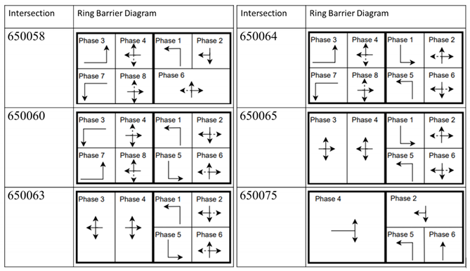
The six signalized intersections cover a wide range of phasing schemes, including four, six, seven, and eight-phase operations, as shown in Table 1. Intersection 650075, which is a T intersection, covers the four-phase operation. Intersections 650063 and 650065 cover a six-phase operation with split phasing for the side road, where each road discharges traffic in all directions in its own phase. Intersection 650058 uses seven phases where the southbound left turn is not allowed. The other two intersections 650060 and 650064 have all eight phases.
The phasing plans shown in the figure do not fully follow the NEMA phasing scheme and they are shown in the same way dictated by the data. Most notably, the two sides of the barrier phases are swapped. This is because phases 2 and 6 are the ending phases for every cycle. This is mainly to allow for the coordination of the end of the arterial through phases with other traffic signals and to allow for serving these phases for the entire cycle when no actuations are received. The data used were obtained from the Virginia SmarterRoads Web portal. The data were broadcasted by the web API every second and we created a script to capture the data in a JSON file format and construct a database of traffic signal timings. The data were generated by traffic signal controllers and contain in-depth information about the state of the controller. Because of communication losses from the controller to the Web API and then from the API to our servers, the data has missing values that can sum up to 30 percent for some days. These missing data are coded as missing values and fed to the model as is without imputation to mimic data losses that happen in infrastructure-to-vehicle communication. Figure 2 describes the unique data elements in the VDOT SmarterRoads data.
It should be noted that the level of complexity of SPaT prediction varies significantly across intersections. This variation can be attributed to many factors, including: traffic signal controller logic, driver behavior, intersection geometry, and phasing schemas. The intersections examined were using D4 traffic signal controllers, and the data used had specific traits that made predictions particularly complex. This includes:
- The sequences of data used have up to 30 percent missing data. This affects the overall accuracy of the predictions but is more representative of realistic infrastructure to vehicle communication streams.
- The controller logic includes significant skipping of left turn and side street phases, which makes the predictions highly stochastic, where a single arrival on the secondary road can completely alter the time to green for the primary road.
- The controller logic for all six intersections includes a setting where, for some cycles, if there are no actuations on any of the approaches, the entire cycle serves phases 2 and 6, which are the primary road through, right and permissive left movements. In this case, the time to green is extended by an entire cycle, which is difficult to predict, especially a long time in advance.
Model Development
Four machine learning models are fitted and compared for tasks 1 and 2, which were introduced at the beginning of the methodology section. This includes three previously used in literature which are: MLP, LSTM, and CNN-LSTM. Another architecture based on Transformer Encoder Blocks is proposed, which will be referred to as the Transformer in this paper for brevity despite it not having the decoder element of a full transformer model
Common Elements
All four models used were implemented in the Pytorch deep learning library [18]. All four models were formulated as regression models with the output having P features, where P is the number of phases being predicted for the intersections. The output features resemble the residual time to green (TTG) or time to red (TTR) in each of the P phases of the traffic signal. The models use the Adam optimizer, which was used by all previous deep-learning models predicting SPaT data. Batch size and learning rate were two general hyperparameters that were tested for all models. All models have the same input, which is an input sequence where F is the number of features and S is the length of the time window chosen to generate the input sequence. After trying multiple values for S including 3, 10, 30, 60, and 120 seconds, respectively, the best results were achieved using a 10-second time window in the past. The Mean Absolute Percentage Error (MAPE) was used as the loss function for all models.
MAPE was used as the loss function for all models. The reason for choosing MAPE is that it penalizes errors much more when the prediction is closer to zero. This allows for increased prediction performance for predictions that are closer in the future. From an application standpoint, the sooner the traffic signal changes, the higher the need for reliable predictions [3]. In a previous study, we analyzed intersection 650065 and showed that the MAPE performs best with short-term predictions, which is the major focus of GLOSA applications [15]. All model hyperparameters were tuned using the Raytune distributed model selection library [19]. The tuning utilizes the Asynchronous Successive Halving (ASHA) algorithm to choose the best hyperparameters that fit the model by employing a selection criterion for aggressive early stopping of less favorable model configurations in favor of more promising configurations to maximize the use of computational resources [20]. Every model type was allowed 8 hours of computational time with 2 Nvidia Tesla A100 GPUs to select the best hyperparameters. The model variants were provided a maximum of 10 epochs for training. The computing node was allowed to train up to 10 model variants in parallel. For each model type, hundreds of configurations were tried to reach the best configurations.
MLP
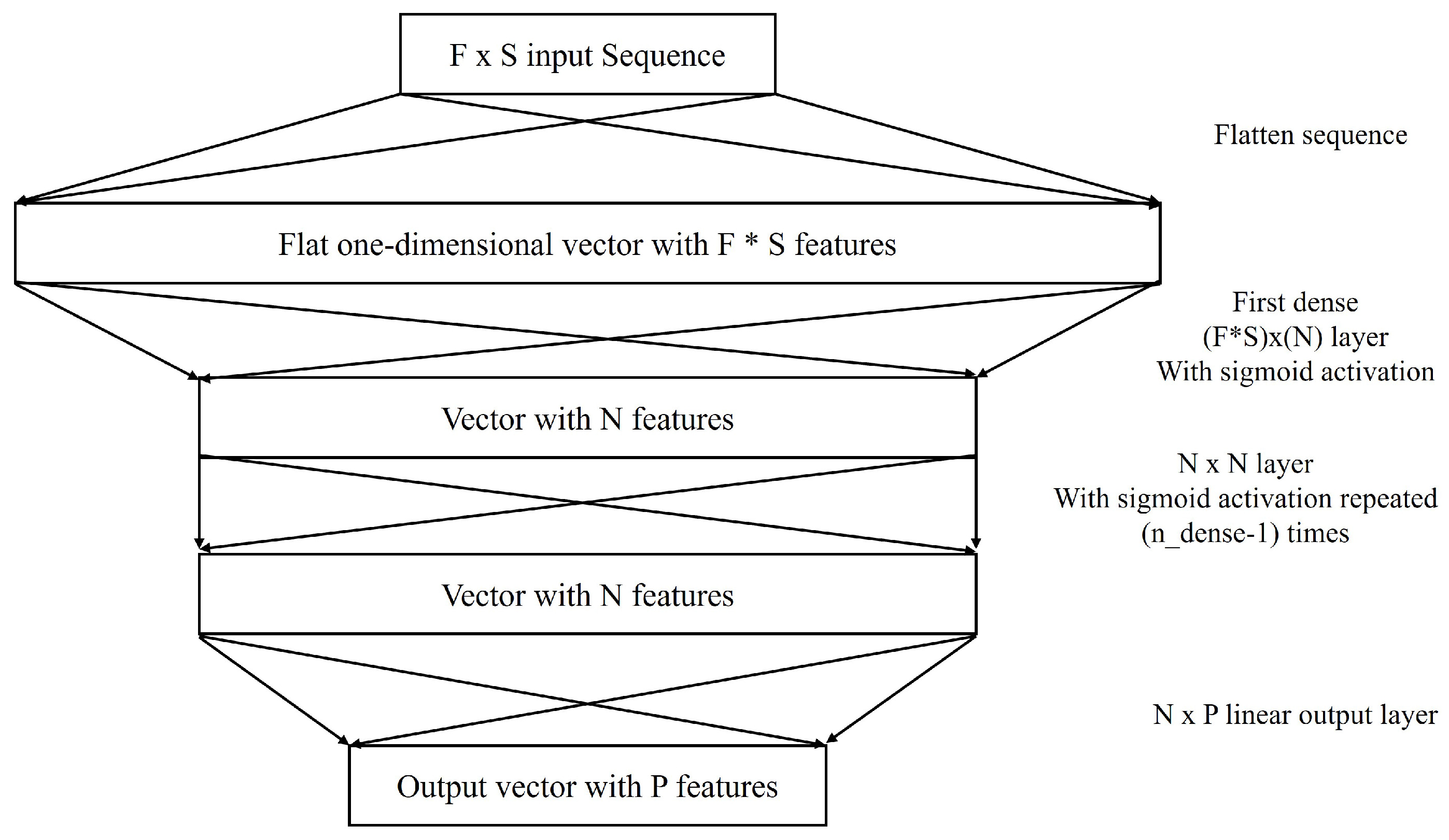
MLPs are the simplest baseline neural network architecture that was tested. This multilayer perceptron implementation took the same input as other models, which is the 10-second sequence of data. The features for each one of the 10-time steps were treated as separate features with separate weights assigned to them. In other words, the model uses data from the last 10 seconds with no context of the order of the data or assigning more value to more recent information. In this case, the model is left on its own to decide on the weights to assign to each variable for each time step, which gives the model more control to access very relevant data that occurred further back in the earlier time steps of the input sequence. The model has two main hyperparameters, which are the number of nodes per layer N and the number of dense layers with sigmoid activation . Other activation functions like ReLu were used and compared with the sigmoid activation function, but the sigmoid activation worked best for this application.
Figure 3.
MLP Neural Network Architecture.
LSTM
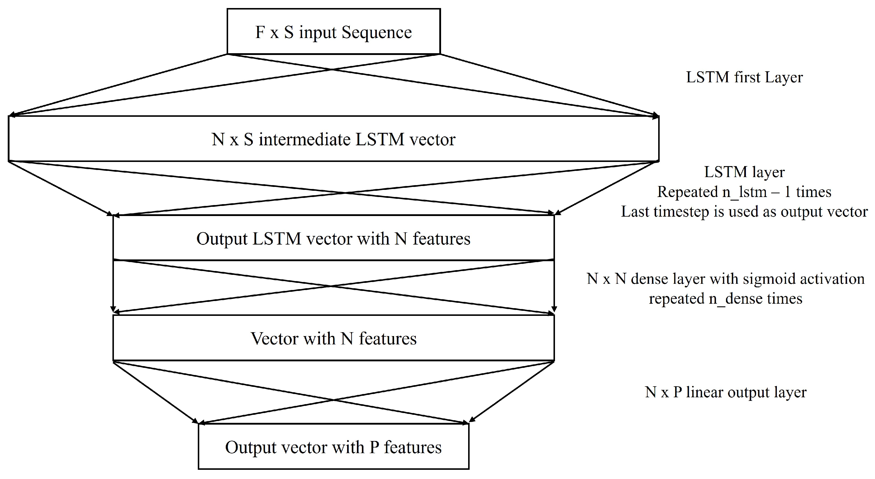
LSTM neural networks have been used in this application multiple times and were one of the best architectures for use with this application [14,15,21]. LSTM acknowledges temporal dependencies between data elements across different time steps. This allows the LSTM neural network to recognize temporal dependencies between signal states and other variables, such as traffic volumes, speeds, vehicle arrivals, and pedestrian arrivals. This facilitates predictions for the network, considering both short-term dependencies and long-term trends within the data. The structure of LSTM used in this study is the one proposed by Graves in 2013 [22]. The LSTM cell can be described using the following five equations:
The variable refers to the input at time t. Input, output, and forget gates are referred to as i, o, and f, respectively. The inner LSTM cell is referred to as c, which is where information is stored. The variable h refers to the hidden state. Weights are referred to as W and biases as b. The Tanh activation is used for the LSTM layers. In this model, there are a total of three main hyperparameters that were tuned. N was used as the number of features of the LSTM sequence, the number of features in the LSTM output vector, and the number of neurons in the dense layer. The variable is the number of LSTM layers. The variable is the number of dense layers with sigmoid activation used to aggregate the LSTM output.
Figure 4.
LSTM Neural Network Architecture.
CNN-LSTM
CNN-LSTM was proposed in a previous study as the best method for SPaT prediction, albeit being very similar in prediction performance to a simple LSTM [16]. Using two-dimensional convolutions, however, was found to not be very useful to aggregate features because, unlike computer vision applications where features are spatially corelated, the controller features are not spatially corelated so the output of the two-dimensional CNN-LSTM would be highly reliant on the exact order of the chosen features. For this reason, one-dimensional CNN-LSTM is better suited for this specific problem, where the convolutions can detect specific trends observed across each feature separately and feed that into the LSTM to capture temporal dependencies. The CNN-LSTM has five different hyperparameters, which include: the filter size C for the convolution, the number of convolution layers number of LSTM layers number of dense layers and the number of neurons in each layer N. N refers to the number of LSTM cells and the number of neurons for the dense layer.
Figure 5.
CNNLSTM Neural Network Architecture.

Transformer
A typical transformer architecture comprises an encoder block to process the inputs and apply self-attention between the input sequence time steps and a decoder block to do the same for the output, such that the mapping between the input and output sequences can be established. The architecture proposed in Figure 6 uses only the encoder block of the transformer and replaces the decoder block with dense layers using sigmoid activations and a final linear layer for regression. The encoder block, in this case, is only used to map the self-attention of the input sequence, since the output is not a sequence, but a simple vector showing the residual time to green or time to red for each phase. The encoder block structure is similar to that described by Vaswani et al. [23]. The main model-specific hyperparameters, in this case, include N, which is the size of the input embedding and also the size of the transformer output and the size of the dense layers prior to the output; , which is the number of attention heads in each encoder multi-headed attention; , which is the number of encoders stacked in the model; and , which is the number of dense layers with sigmoid activations to aggregate the transformer encoders’ output before the output linear layer. The transformer encoder block architecture is shown in Figure 7, which is adapted from Viswani et al. [23].
Figure 6.
Transformer encoder-based Architecture.
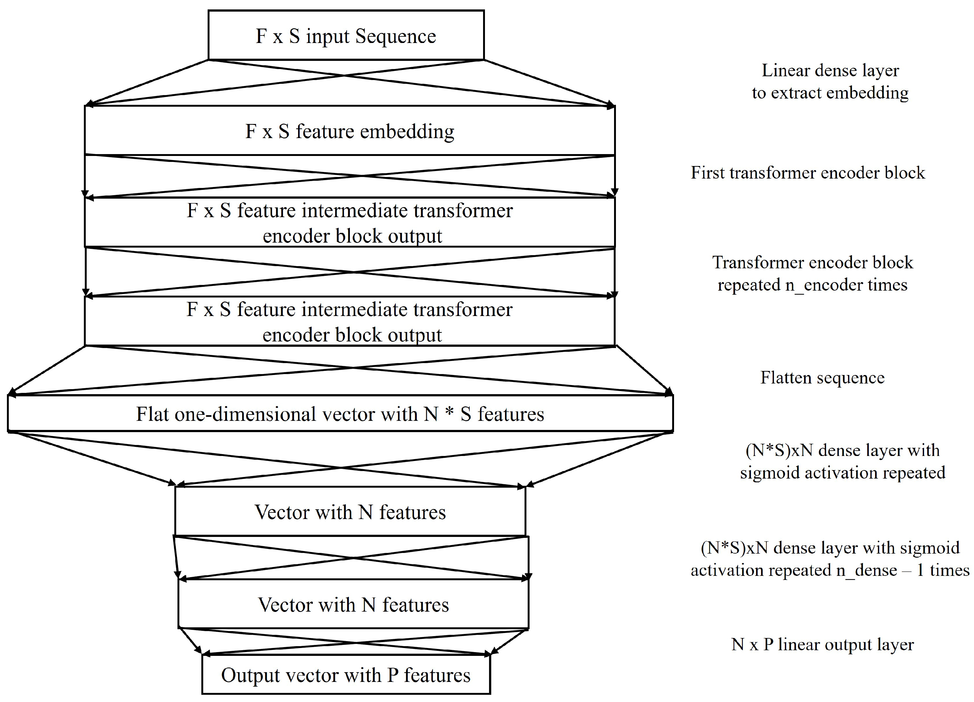
Figure 7.
Encoder block architecture.
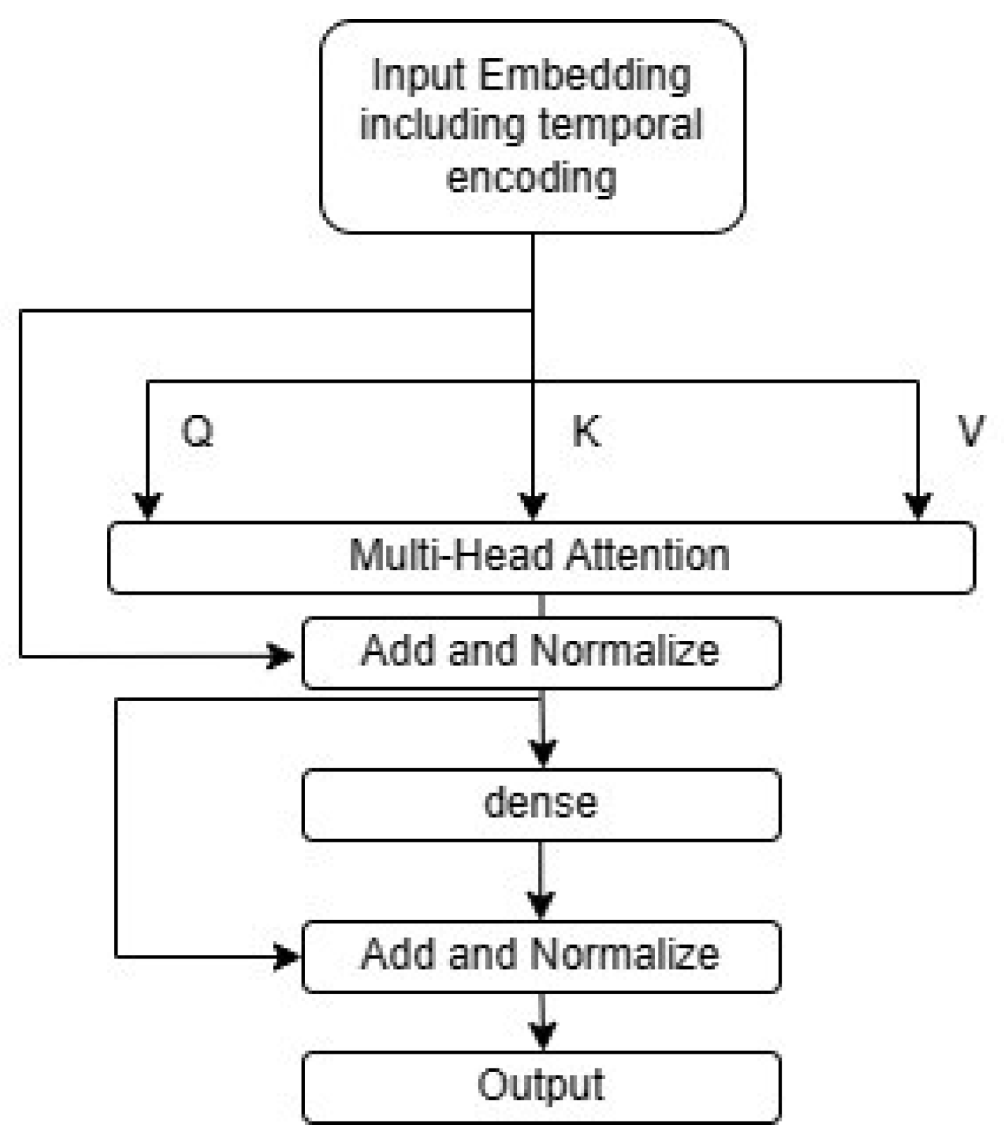
The variables Q, K, and V in this case represent the query, key, and value, which are linear projections of the input embedding that includes the temporal encoding for each attention head. For each head, the dot product attention can be computed as [23]:
Where the matrix multiplication between Q and K is a measure of similarity between the query and key matrices. This is divided by a scaling factor equal to the square root of the dimension of the key matrix for normalization. The purpose of this dot product attention between Q and K, which are linear projections of the input sequence, is self-attention. The dot product is a similarity metric between Q and K, which allows the model to distinguish which time steps are more relevant to the prediction of time to change and which are less relevant. Finally, this is subjected to the softmax function to magnify differences between self-attention weights to help the model decide which time steps are most relevant to the prediction. This is then multiplied by the value matrix to get the output of the dot product attention, which has all the features with a special focus on the timesteps that are most relevant to the prediction.
Ensemble Approach
The four models used MLP, LSTM, CNN-LSTM, and Transformer vary significantly in how they handle data and the computations they require to make a prediction. We can make use of this variation in model logic in making an ensemble-based prediction. One of the main prerequisites for a successful ensemble model is having diversity in the ensemble constituent models [24]. This is achieved in two ways:
- By using four different architectures, the data is subjected to different processes and logic in order to extract the relevant features and make the prediction. This variance in logic, as represented by the different model architectures, adds to the logical diversity of the model.
- For each of the four models, during hyperparameter tuning we generate multiple variants where the number of parameters used to express the model for each variant varies significantly. This means that the variation of model size and number of parameters, even for the same model architecture, allows for diversity in the complexity of the constituent models for the ensemble.
Using the ensemble approach for the prediction of SPaT information is hypothesized to have two key sources of value: Hypothesis 1: Using multiple diverse predictions instead of one is likely to improve prediction performance by eliminating outlier predictions, which are ’model hallucinations’. The constituent models of the ensemble are unlikely to provide the same incorrect prediction whether that error is because of bias or variance unless the bias or variance is inherent to the data and has nothing to do with the model.
Hypothesis 2: For each prediction, reporting consensus between the constituent models of the ensemble can serve as a powerful indicator of confidence in the prediction. This means that predictions agreed upon by more models are more likely to be closer to the true value. This can be easily tested by looking at the error distribution of different predictions and how it varies with consensus between the models. The expected behavior is that as consensus increases, the mean error of the predictions should decrease, and the percentage of distant outlier predictions should decrease.
3. Results and Analysis
This section is subdivided into three subsections, presenting the results for the three tasks outlined at the beginning of the methodology. This helps us better understand how well the models perform on each task and how that affects the overall performance of the ensemble prediction. Each of the three tasks is carried out using the top three ranked models of each architecture, totaling 12 different models. The models are ranked based on the Mean Absolute Percentage Error (MAPE). Table 2 to Table 5 provide the hyperparameter configuration of the top-ranked 12 models for each of the 6 intersections.
Table 2 through Table 5 show that for each model, for each intersection, there is a variation between the top three chosen models in terms of the hyperparameters. This variation leads to the diversity of the top three selected models, which is what allows the top three models to be useful for the model ensemble
3.1. Task 1: Identifying Change Times Less than 20 Seconds in the Future:
The task aims to distinguish between predictions less than 20 seconds ahead and those further in the future. Each of the 12 models makes a regression prediction, which is then converted to a binary outcome: 1 if under 20 seconds, 0 if over. Regression models are used for their superior performance in classification due to their nuanced loss function. Three ensemble techniques are tested: mean, median, and majority vote of the 12 models. The table shows the classification accuracy for each model at each intersection and the ensemble methods.
Table 6 shows all architectures achieve accuracies around 95%. The transformer architecture outperforms others at all intersections except for 650075, where the MLP slightly outperforms the transformer. The MLP is the second-best model, demonstrating that treating sequence time steps as separate features is effective. LSTM is the second worst, and CNN-LSTM is the worst. The best overall performance is achieved by taking the mean of the 12 models compared to the 20-second cutoff, resulting in the highest accuracy at all intersections except 650058 and 650064, where it is slightly outperformed by the best transformer model. Median and voting strategies are outperformed by the best transformer model for all intersections.

Table 2.
MLP best model configurations
| Intersection | Model Rank | lr | Batch size | Neurons per layer | n layers |
|---|---|---|---|---|---|
| 650058 | 1 | 0.00019 | 16 | 300 | 2 |
| 2 | 0.00029 | 16 | 240 | 2 | |
| 3 | 0.00042 | 32 | 240 | 2 | |
| 650060 | 1 | 0.00062 | 64 | 300 | 2 |
| 2 | 0.00046 | 32 | 270 | 2 | |
| 3 | 0.00026 | 16 | 240 | 2 | |
| 650063 | 1 | 0.00025 | 32 | 210 | 2 |
| 2 | 0.00035 | 16 | 150 | 2 | |
| 3 | 0.00092 | 128 | 240 | 4 | |
| 650064 | 1 | 0.00025 | 16 | 210 | 2 |
| 2 | 0.00019 | 16 | 300 | 2 | |
| 3 | 0.00046 | 32 | 270 | 2 | |
| 650065 | 1 | 0.00041 | 32 | 270 | 2 |
| 2 | 0.00045 | 64 | 210 | 2 | |
| 3 | 0.00019 | 16 | 240 | 2 | |
| 650075 | 1 | 0.00032 | 16 | 150 | 2 |
| 2 | 0.00040 | 16 | 210 | 1 | |
| 3 | 0.00105 | 64 | 180 | 2 |
3.2. Task 2: Predicting the Exact Time to Change When Less than or Equal to 20 Seconds
After deciding whether the time to change for each phase is within 20 seconds in the future. The next task is to predict the exact time to change for each phase. Table 7 and Table 8 show the MAPE and mean absolute error for each model for the subset of data with time-to-change less than 20 seconds in the future for all six intersections. The prediction performance of the mean and median of the model ensemble is also provided in both tables.
Table 7 and Table 8 both show that the proposed transformer-encoder-based architecture outperforms all the other architectures for all intersections except for intersection 650060 where CNN-LSTM outperforms the transformer architecture. Aside from intersection 650060, CNN-LSTM is slightly outperformed by MLP. Vanilla LSTM is the worst performing by a small margin. All architectures have reasonably low MAPE between 11 and 23 percent, meaning that the absolute error is between 11 and 23 percent of the predicted value. This results in the best models being off by 0.96 seconds from the true value on average and that the worst are about 2.05 seconds from the true value on average, as shown in Table 8. The ensemble shows that taking the mean, or the median value of all models, enhances the prediction. The median value, however, is the best estimator for the prediction because it is robust to outliers, unlike the mean. The median value always leads to a non-trivial improvement over the best model prediction across all 12 models. This proves hypothesis 1 outlined at the end of the methodology section. By taking the median of the predictions of 12 diverse models, the hallucinations of a subset of the models can be rectified, leading to an overall better prediction performance and a result that outperforms every individual model.
Table 3.
LSTM best model configurations
| Intersection | Model Rank | lr | batch size | neurons per layer | n layers lstm | n layers dense |
|---|---|---|---|---|---|---|
| 650058 | 1 | 0.00134 | 128 | 300 | 2 | 1 |
| 2 | 0.00135 | 128 | 210 | 2 | 1 | |
| 3 | 0.00068 | 32 | 120 | 2 | 1 | |
| 650060 | 1 | 0.00111 | 32 | 180 | 2 | 1 |
| 2 | 0.00134 | 128 | 300 | 2 | 1 | |
| 3 | 0.00168 | 64 | 180 | 2 | 1 | |
| 650063 | 1 | 0.00024 | 16 | 180 | 2 | 2 |
| 2 | 0.00040 | 32 | 180 | 2 | 1 | |
| 3 | 0.00068 | 32 | 120 | 2 | 1 | |
| 650064 | 1 | 0.00068 | 32 | 120 | 2 | 1 |
| 2 | 0.00119 | 32 | 120 | 2 | 2 | |
| 3 | 0.00120 | 32 | 150 | 1 | 1 | |
| 650065 | 1 | 0.00040 | 32 | 180 | 2 | 1 |
| 2 | 0.00139 | 32 | 150 | 2 | 1 | |
| 3 | 0.00068 | 32 | 120 | 2 | 1 | |
| 650075 | 1 | 0.00034 | 16 | 90 | 2 | 2 |
| 2 | 0.00111 | 32 | 180 | 2 | 1 | |
| 3 | 0.00068 | 32 | 120 | 2 | 1 |
3.3. Task 3: Assigning a Level of Certainty to the Prediction
The third task, which is the most important and the least addressed in the literature, is to assign a level of certainty to each prediction. For each input and phase, the 12 best models provide a prediction. Due to model errors from bias and variance, models are unlikely to converge on the same incorrect prediction unless there is an inherent data error.
A certainty metric is defined based on model consensus. Given a set of predictions P for the same input with a median prediction m, an adjustable tolerance level t (typically within 20 percent) is used. The number of predictions within this tolerance indicates the certainty level. Certainty is computed by the number or percentage of agreeing models. The number of models in consensus is preferred over the percentage, as the latter could be misinterpreted as the probability of a correct prediction.
Testing this formulation, a tolerance level of 5% is chosen and the count of the models within this tolerance level is evaluated. This results in 12 different levels of confidence from 1 to 12, where 1 indicates the least confidence (a minimum of 1 model agrees with this median within tolerance) and 12 indicates the highest confidence (all 12 models agree on this median within tolerance). The MAPE levels for each level of consensus are shown in Figure 8. It should be noted that for each level of consensus, the error shown is for this level of consensus or higher, so a level of consensus of 1 shows the overall MAPE as the entire dataset has a minimum level of consensus of 1 model.
Figure 8 highlights the effectiveness of the consensus metric in distinguishing high-confidence from low-confidence predictions. Intersection 650058 has a 16.04% MAPE overall, which drops to 3.59% when all 12 models reach consensus. At intersection 650060, the MAPE decreases by 80%, from 16.83% to 3.2%, for the highest consensus score. For intersection 650063, the MAPE falls from 16.89% to 5.33% with a consensus score of 12, confirming hypothesis 2 from the methodology section. The consensus score quantifies prediction uncertainty before the true value is known. This approach is adaptable to all model types, including statistical and machine learning models, and can be combined with other certainty measures like probabilistic predictions. Figure 8 shows the error probability distribution for each consensus level from 1 to 12. The error is computed using the equation:
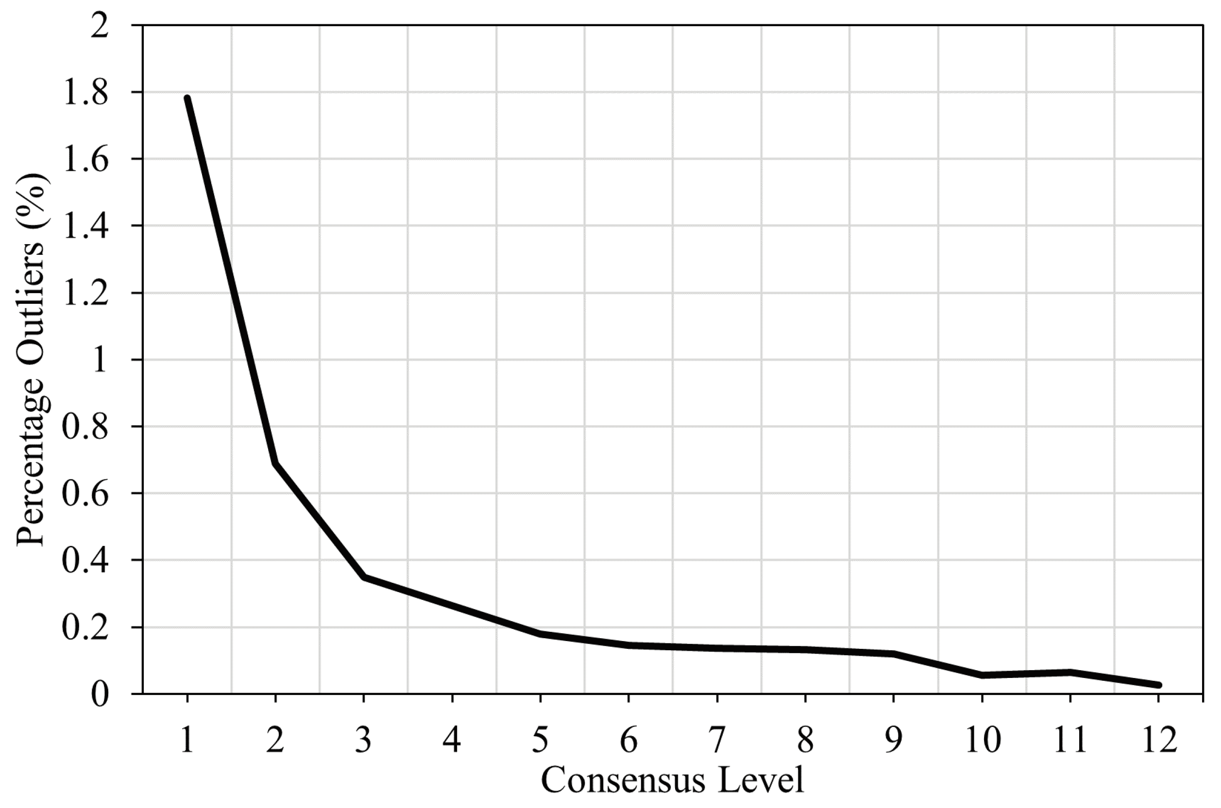
Where is the median of the model predicted values and is the ground truth. This means that a positive error refers to an overestimation and a negative error refers to an underestimation of the traffic signal time to change. The error distribution shown in Figure 8 shows errors between -10 seconds and +10 seconds for the 20-second prediction window. Errors greater than 10 seconds are distant outliers and their percentages for each level of consensus are shown in Table 8 for completeness. Errors are aggregated across all six intersections. The predictions are all rounded to the nearest second and the ground truth is in seconds. This means that the shown values for each bar in the histograms in Figure 8 are the exact value of the error. For example, the middle bar represents the percentage of the time where the error is zero, so the rounded prediction is exactly equal to the ground truth.
Table 4.
CNNLSTM best model configurations
| Intersection | Model Rank | lr | batch size | neurons per layer | n layers lstm | n layers dense |
|---|---|---|---|---|---|---|
| 650058 | 1 | 0.00040 | 16 | 300 | 2 | 1 |
| 2 | 0.00101 | 32 | 240 | 2 | 1 | |
| 3 | 0.00109 | 64 | 240 | 2 | 1 | |
| 650060 | 1 | 0.00080 | 32 | 300 | 4 | 1 |
| 2 | 0.00021 | 16 | 300 | 4 | 1 | |
| 3 | 0.00040 | 16 | 300 | 2 | 1 | |
| 650063 | 1 | 0.00109 | 64 | 240 | 2 | 1 |
| 2 | 0.00061 | 16 | 120 | 4 | 1 | |
| 3 | 0.00048 | 32 | 300 | 2 | 1 | |
| 650064 | 1 | 0.00253 | 128 | 240 | 3 | 1 |
| 2 | 0.00050 | 16 | 120 | 3 | 1 | |
| 3 | 0.00230 | 128 | 210 | 4 | 1 | |
| 650065 | 1 | 0.00041 | 16 | 240 | 4 | 1 |
| 2 | 0.00121 | 128 | 150 | 4 | 1 | |
| 3 | 0.00050 | 16 | 120 | 3 | 1 | |
| 650075 | 1 | 0.00041 | 16 | 240 | 4 | 1 |
| 2 | 0.00080 | 32 | 300 | 4 | 1 | |
| 3 | 0.00168 | 64 | 120 | 2 | 1 |
Table 5.
Transformer best model configurations
| Intersection | Model Rank | lr | batch size | embed dim (N) | n heads | n encoder layers | n layers dense |
|---|---|---|---|---|---|---|---|
| 650058 | 1 | 0.00020 | 32 | 300 | 1 | 2 | 2 |
| 2 | 0.00016 | 32 | 240 | 3 | 1 | 4 | |
| 3 | 0.00014 | 32 | 210 | 2 | 2 | 2 | |
| 650060 | 1 | 0.00018 | 16 | 60 | 3 | 2 | 2 |
| 2 | 0.00046 | 64 | 90 | 3 | 2 | 4 | |
| 3 | 0.00042 | 32 | 60 | 5 | 2 | 2 | |
| 650063 | 1 | 0.00067 | 64 | 30 | 5 | 4 | 2 |
| 2 | 0.00080 | 128 | 60 | 5 | 1 | 2 | |
| 3 | 0.00018 | 16 | 60 | 3 | 2 | 2 | |
| 650064 | 1 | 0.00014 | 32 | 210 | 2 | 2 | 2 |
| 2 | 0.00020 | 32 | 300 | 1 | 2 | 2 | |
| 3 | 0.00046 | 64 | 120 | 1 | 1 | 2 | |
| 650065 | 1 | 0.00075 | 128 | 150 | 1 | 1 | 2 |
| 2 | 0.00041 | 128 | 120 | 3 | 1 | 2 | |
| 3 | 0.00024 | 32 | 210 | 1 | 1 | 4 | |
| 650075 | 1 | 0.00029 | 32 | 120 | 1 | 1 | 4 |
| 2 | 0.00020 | 32 | 300 | 1 | 2 | 2 | |
| 3 | 0.00018 | 16 | 60 | 3 | 2 | 2 |
Figure 8.
MAPE as a function of the level of consensus with a 5% tolerance level for all 6 intersections.
Figure 8.
MAPE as a function of the level of consensus with a 5% tolerance level for all 6 intersections.
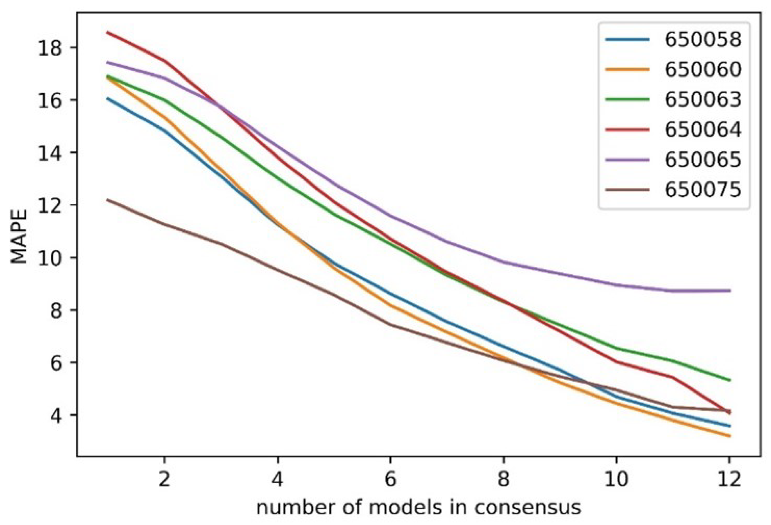
Figure 9 and Figure 10 illustrate the error distributions for different consensus levels at a 5 percent tolerance. Lower consensus levels have flatter error curves. At a consensus level of 1, the median prediction has zero error 36% of the time, while at level 12, it has zero error 61% of the time. The error is within 1 second 90.2% of the time at level 12 but only 68.4% at level 1. The ensemble’s error exceeds 10 seconds 1.782% of the time at level 1, compared to just 0.026% at level 12. Thus, at level 1, the ensemble is 68.5 times more likely to be off by more than 10 seconds than at level 12. This strongly supports hypothesis 2, showing that the consensus level is a reliable indicator of prediction accuracy.
Table 6.
Classification accuracy of different models distinguishing whether a signal phase will change 20 seconds in the future
Table 6.
Classification accuracy of different models distinguishing whether a signal phase will change 20 seconds in the future
| Intersection | Model | LSTM | MLP | CNN- | Trans- | Mean | Median | Vote |
|---|---|---|---|---|---|---|---|---|
| Rank | LSTM | former | ||||||
| 650058 | 1 | 94.84% | 94.97% | 94.37% | 95.31% | 95.24% | 95.12% | 95.08% |
| 2 | 94.59% | 94.71% | 94.63% | 95.25% | ||||
| 3 | 94.68% | 94.82% | 94.64% | 95.14% | ||||
| 650060 | 1 | 95.20% | 95.23% | 93.47% | 95.04% | 95.53% | 95.03% | 95.17% |
| 2 | 94.40% | 95.11% | 93.22% | 95.09% | ||||
| 3 | 94.20% | 95.05% | 93.58% | 95.32% | ||||
| 650063 | 1 | 95.95% | 95.90% | 95.88% | 96.07% | 96.17% | 96.10% | 96.08% |
| 2 | 95.70% | 96.01% | 95.54% | 95.96% | ||||
| 3 | 95.87% | 95.84% | 95.91% | 96.04% | ||||
| 650064 | 1 | 94.98% | 95.84% | 94.20% | 96.59% | 96.51% | 96.04% | 96.17% |
| 2 | 95.06% | 95.81% | 93.77% | 96.24% | ||||
| 3 | 95.67% | 95.97% | 94.36% | 96.45% | ||||
| 650065 | 1 | 95.63% | 96.36% | 94.33% | 96.39% | 96.43% | 96.08% | 96.07% |
| 2 | 95.88% | 95.75% | 94.18% | 96.35% | ||||
| 3 | 95.76% | 95.92% | 94.39% | 96.08% | ||||
| 650075 | 1 | 96.01% | 96.63% | 96.01% | 96.07% | 96.73% | 96.07% | 95.86% |
| 2 | 96.08% | 96.19% | 95.54% | 96.18% | ||||
| 3 | 95.77% | 96.05% | 95.59% | 96.04% |
Figure 9.
The error distributions a) consensus values 1 to 3. b) consensus values 4 to 6. c) consensus values 7 to 9. d) consensus values 10 to 12.
Figure 9.
The error distributions a) consensus values 1 to 3. b) consensus values 4 to 6. c) consensus values 7 to 9. d) consensus values 10 to 12.
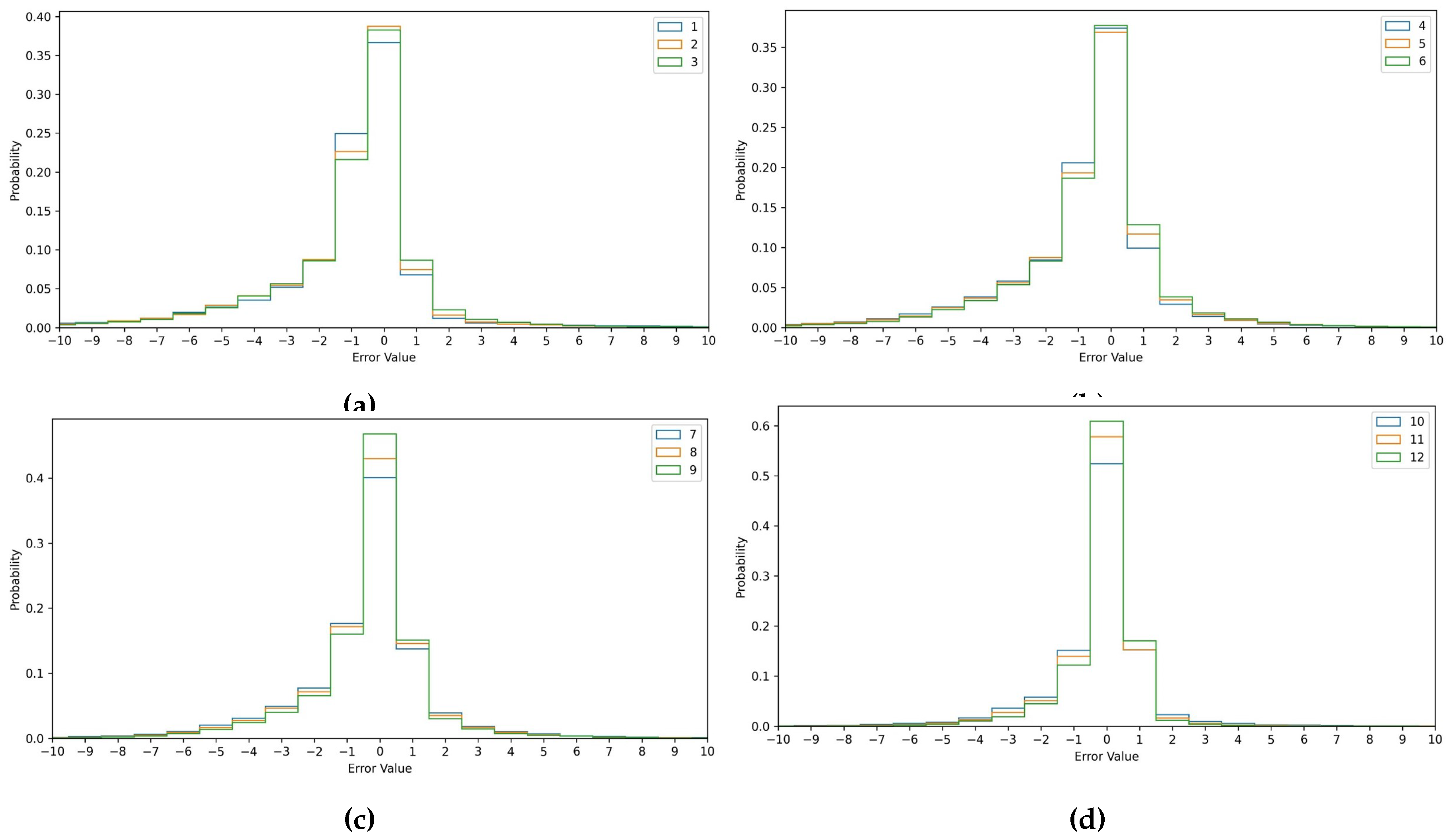
Table 7.
Mean Absolute Percentage Error of Each Model for Values under 20 seconds
| Inter- section | Model Rank | LSTM | MLP | CNN- LSTM | Trans- former | Mean | Median |
|---|---|---|---|---|---|---|---|
| 650058 | 1 | 20.45 | 16.65 | 19.40 | 15.39 | 15.58 | 15.03 |
| 2 | 19.70 | 16.33 | 20.43 | 15.95 | |||
| 3 | 21.15 | 16.68 | 20.90 | 15.29 | |||
| 650060 | 1 | 22.64 | 19.49 | 17.80 | 18.07 | 16.72 | 15.89 |
| 2 | 20.90 | 19.12 | 17.84 | 19.01 | |||
| 3 | 21.79 | 19.29 | 20.27 | 19.03 | |||
| 650063 | 1 | 22.47 | 19.65 | 20.62 | 16.29 | 16.45 | 15.61 |
| 2 | 23.14 | 19.20 | 18.67 | 16.90 | |||
| 3 | 22.47 | 19.19 | 21.23 | 17.56 | |||
| 650064 | 1 | 22.29 | 21.28 | 21.92 | 19.88 | 18.31 | 17.60 |
| 2 | 23.08 | 21.18 | 22.43 | 18.75 | |||
| 3 | 25.07 | 22.58 | 23.09 | 19.38 | |||
| 650065 | 1 | 22.74 | 19.97 | 19.65 | 17.56 | 16.70 | 16.32 |
| 2 | 22.21 | 18.97 | 19.82 | 17.90 | |||
| 3 | 22.54 | 19.19 | 20.33 | 17.34 | |||
| 650075 | 1 | 16.38 | 15.01 | 12.95 | 11.37 | 11.94 | 10.99 |
| 2 | 17.64 | 13.68 | 14.96 | 13.25 | |||
| 3 | 17.62 | 13.64 | 16.25 | 12.94 |
Figure 10.
Percentage of outlier predictions with an error greater than 10 seconds
3.4. Fuel Consumption
To further quantify the effect of the consensus level on the overall performance of the GLOSA system, the effect on a single vehicle going through an intersection is simulated using the stochastic control algorithm developed by Shafik et al. [3]. The effect of the level of consensus on fuel consumption is shown in Figure 11.
Table 8.
Mean Absolute Error of Each Model for Values under 20 seconds
| Inter- section | Model Rank | LSTM | MLP | CNN- LSTM | Trans- former | Mean | Median |
|---|---|---|---|---|---|---|---|
| 650058 | 1 | 1.585 | 1.456 | 1.572 | 1.345 | 1.330 | 1.309 |
| 2 | 1.509 | 1.450 | 1.707 | 1.428 | |||
| 3 | 1.636 | 1.480 | 1.614 | 1.351 | |||
| 650060 | 1 | 1.839 | 1.720 | 1.516 | 1.684 | 1.483 | 1.419 |
| 2 | 1.619 | 1.728 | 1.501 | 1.760 | |||
| 3 | 1.677 | 1.773 | 1.621 | 1.718 | |||
| 650063 | 1 | 1.785 | 1.647 | 1.711 | 1.473 | 1.446 | 1.428 |
| 2 | 1.786 | 1.695 | 1.632 | 1.511 | |||
| 3 | 1.776 | 1.662 | 1.702 | 1.573 | |||
| 650064 | 1 | 1.843 | 1.909 | 1.864 | 1.801 | 1.644 | 1.615 |
| 2 | 1.945 | 1.898 | 1.917 | 1.685 | |||
| 3 | 2.051 | 2.052 | 1.954 | 1.782 | |||
| 650065 | 1 | 1.836 | 1.659 | 1.776 | 1.605 | 1.502 | 1.496 |
| 2 | 1.757 | 1.688 | 1.811 | 1.595 | |||
| 3 | 1.821 | 1.671 | 1.762 | 1.556 | |||
| 650075 | 1 | 1.177 | 1.194 | 1.033 | 0.962 | 0.933 | 0.888 |
| 2 | 1.264 | 1.086 | 1.247 | 1.056 | |||
| 3 | 1.213 | 1.074 | 1.168 | 1.005 |
Figure 11.
Effect of level of consensus on fuel savings.
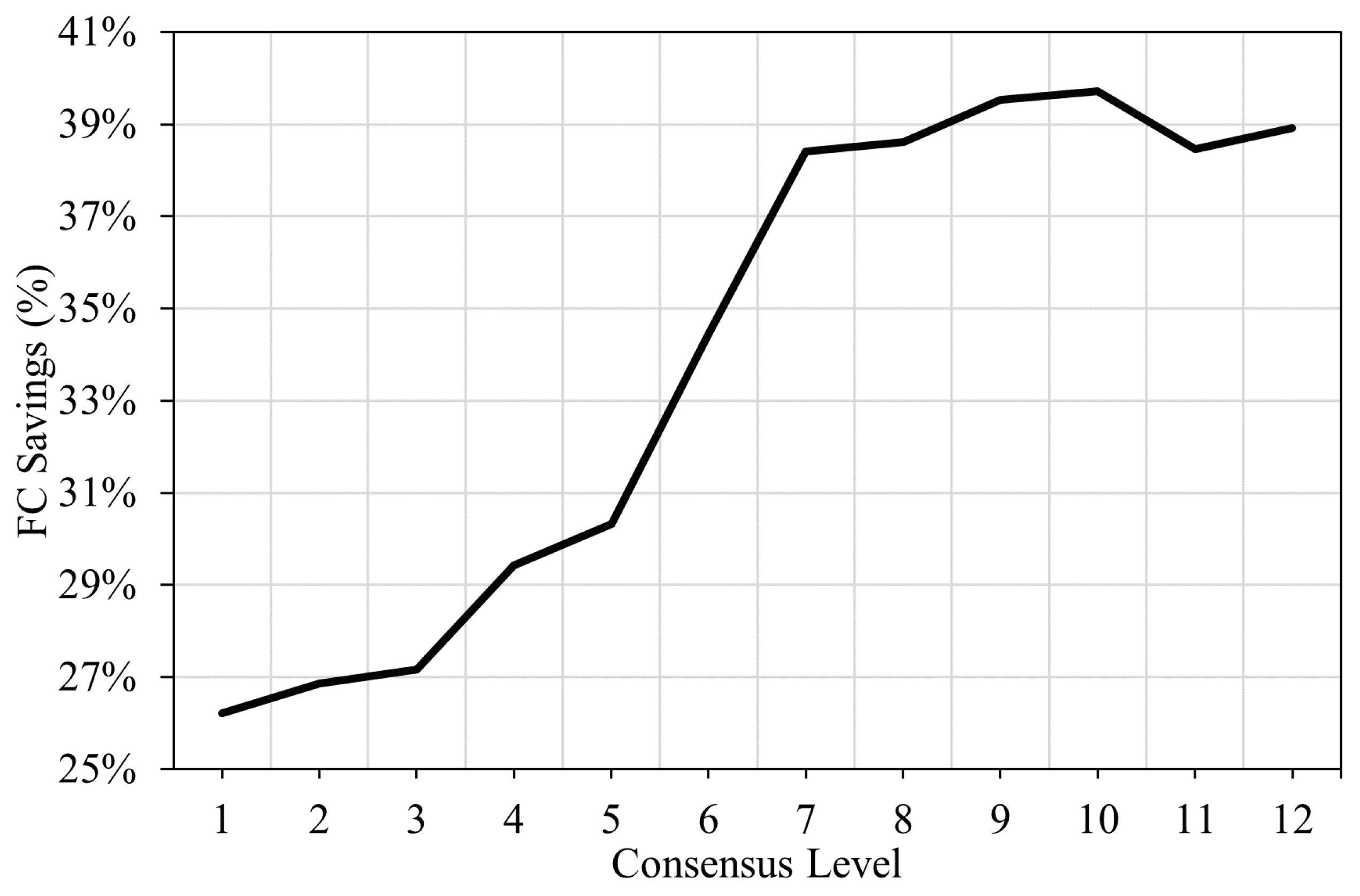
Figure 11 shows that if more than half the models agree on the prediction (level of consensus of 7 or more), the maximum level of fuel savings of about 40 percent can be achieved compared to uninformed driver behavior obtained from field data from Chen et al. [6]. The fuel savings continue to decrease as the level of consensus of the model decreases with the lowest level of consensus achieving about 26 percent in fuel savings.
4. Conclusion and Recommendation
This study proposed a transformer encoder-based architecture in order to enhance SPaT data through better predictions of traffic signal switch times and provide levels of confidence in these predictions for use in GLOSA applications. The transformer was compared against other architectures previously used in the literature, which include MLP, LSTM, and CNN-LSTM. The transformer was found to outperform the other three architectures in two different tasks related to GLOSA. These are predicting whether a specific phase would change within the next 20 seconds and predicting the exact changing time within that period. Three variants of each model type were integrated into an extensible ensemble framework. The ensemble was proven to improve the overall prediction performance to be better than the best model performance by reducing model hallucinations by taking the mean of all models to identify a change time within 20 seconds and the median for prediction of the actual switch time within the 20-second window. The consensus of models is a good indicator of the quality of predictions and the certainty in the predictions. The highest confidence predictions had as much as an 80 percent reduction in MAPE compared to the lowest confidence prediction. The level of consensus can provide a much-needed estimation of the confidence in the most likely switching time in the SPaT messages. Future areas of study might examine the field-testing of ensemble predictions and consensus-based certainty in a transportation network. Issues such as communication latencies, interference, queueing and vehicle dynamics can affect the degree to which the vehicles can benefit from enhanced SPaT messages. Quantifying the error in the SPaT predictions opens the door for more nuanced error-aware eco-driving that considers the certainty level in the prediction and balances the risks and rewards associated with following the SPaT predictions.
Author Contributions
Conceptualization, H.A.R., and S.E; methodology, H.A.R., H.M.A. and S.E.; software, S.E; validation, S.E., A.K.S., H.M.A., and H.A.R.; formal analysis, S.E., H.M.A., A.K.S., and H.A.R.; data curation, S.E.; writing—original draft preparation, S.E., A.K.S.; writing—review and editing, H.A.R., H.M.A.; visualization, S.E., A.K.S. All authors have read and agreed to the published version of the manuscript.
Funding
This research was funded by the Sustainable Mobility and Accessibility Regional Transportation Equity Research Center, Morgan State University.
Institutional Review Board Statement
Not applicable.
Informed Consent Statement
Not applicable.
Acknowledgments
This effort was funded by the Sustainable Mobility and Accessibility Regional Transportation Equity Research (SMARTER) Center.
Conflicts of Interest
The authors declare no conflicts of interest. The funders had no role in the design of the study; in the collection, analyses, or interpretation of data; in the writing of the manuscript; or in the decision to publish the results.
Abbreviations
The following abbreviations are used in this manuscript:
| TSC | Traffic Signal Control |
| SPaT | Signal phase and timing |
| GLOSA | Green light optimal speed advisory |
| MLP | Multilayer perceptrons |
| LSTM | long-short-term memory neural networks |
| CNNLSTM | Convolutional long-short term memory neural networks |
| I2V | infrastructure to vehicle |
| ITS | intelligent transportation systems |
| DSRC | Dedicated short-range communications |
| LTE | Long-Term Evolution |
| MAPE | Mean Absolute Percentage Error |
| ASHA | Asynchronous Successive Halving |
| GPU | Graphics processing unit |
| NEMA | National Electrical Manufacturers Association |
| TTG | Time to green |
| TTR | Time to red |
| XGB | extreme gradient boosting |
| GRU | gated recurrent units |
References
- Abernethy, B.; Andrews, S.; Pruitt, G. Signal phase and timing (SPaT) applications, communications requirements, communications technology potential solutions, issues and recommendations. Technical report, United States. Federal Highway Administration, 2012.
- Rakha, H.; Kamalanathsharma, R.K. Eco-driving at signalized intersections using V2I communication. Institute of Electrical and Electronics Engineers Inc., 2011, IEEE Conference on Intelligent Transportation Systems, Proceedings, ITSC, pp. 341–346. [CrossRef]
- Shafik, A.K.; Eteifa, S.; Rakha, H.A. Optimization of Vehicle Trajectories Considering Uncertainty in Actuated Traffic Signal Timings. IEEE Transactions on Intelligent Transportation Systems 2023. [CrossRef]
- Rakha, H.; Ahn, K.; Kamalanathsharma, R.K. Eco-vehicle speed control at signalized intersections using i2v communication. US Department of Transportation, Tech. Rep. 2012.
- Kamalanathsharma, R.K.; Rakha, H.A. Multi-stage dynamic programming algorithm for eco-speed control at traffic signalized intersections. IEEE, 2013, pp. 2094–2099.
- Chen, H.; Rakha, H.A.; Loulizi, A.; El-Shawarby, I.; Almannaa, M.H. Development and Preliminary Field Testing of an In-Vehicle Eco-Speed Control System in the Vicinity of Signalized Intersections. IFAC-PapersOnLine 2016, 49, 249–254. [CrossRef]
- Ahn, K.; Du, J.; Farag, M.; Rakha, H.A. Evaluating an Eco-Cooperative Automated Control System. Transportation Research Record 2023, 2677, 1562–1578. [CrossRef]
- Yang, H.; Ala, M.V.; Rakha, H.A. Eco-Cooperative Adaptive Cruise Control at Signalized Intersections Considering Queue Effects. 2016. [CrossRef]
- Bodenheimer, R.; Brauer, A.; Eckhoff, D.; German, R. Enabling GLOSA for adaptive traffic lights. IEEE, 2014, pp. 167–174.
- Ibrahim, S.; Kalathil, D.; Sanchez, R.O.; Varaiya, P. Estimating phase duration for SPaT messages. IEEE Transactions on Intelligent Transportation Systems 2018, 20, 2668–2676.
- Van de Vyvere, B.; D’haene, K.; D’haene, K.; Colpaert, P.; Verborgh, R. Predicting phase durations of traffic lights using live Open Traffic Lights data. Technical University of Aachen, 2019, pp. 1–7.
- Moghimi, B.; Safikhani, A.; Kamga, C.; Hao, W.; Ma, J. Short-term prediction of signal cycle on an arterial with actuated-uncoordinated control using sparse time series models. IEEE Transactions on Intelligent Transportation Systems 2018, 20, 2976–2985. [CrossRef]
- Weisheit, T.; Hoyer, R. Prediction of Switching Times of Traffic Actuated Signal Controls Using Support Vector Machines. In Advanced Microsystems for Automotive Applications 2014; Springer, 2014; pp. 121–129.
- Genser, A.; Ambühl, L.; Yang, K.; Menendez, M.; Kouvelas, A. Time-to-Green predictions: A framework to enhance SPaT messages using machine learning. IEEE, 2020, pp. 1–6.
- Eteifa, S.; Rakha, H.A.; Eldardiry, H. Predicting coordinated actuated traffic signal change times using long short-term memory neural networks. Transportation Research Record 2021, 2675, 127–138. [CrossRef]
- Islam, Z.; Abdel-Aty, M.; Mahmoud, N. Using CNN-LSTM to predict signal phasing and timing aided by High-Resolution detector data. Transportation research part C: emerging technologies 2022, 141, 103742. [CrossRef]
- Farag, M.M.; Rakha, H.A.; Mazied, E.A.; Rao, J. Integration large-scale modeling framework of direct cellular vehicle-to-all (c-v2x) applications. Sensors 2021, 21, 2127. [CrossRef]
- Paszke, A.; Gross, S.; Massa, F.; Lerer, A.; Bradbury, J.; Chanan, G.; Killeen, T.; Lin, Z.; Gimelshein, N.; Antiga, L.; et al. PyTorch: An Imperative Style, High-Performance Deep Learning Library. In Proceedings of the Advances in Neural Information Processing Systems. Curran Associates, Inc., 2019, Vol. 32.
- Liaw, R.; Liang, E.; Nishihara, R.; Moritz, P.; Gonzalez, J.E.; Stoica, I. Tune: A research platform for distributed model selection and training. arXiv preprint arXiv:1807.05118 2018.
- Li, L.; Jamieson, K.; Rostamizadeh, A.; Gonina, E.; Ben-Tzur, J.; Hardt, M.; Recht, B.; Talwalkar, A. A system for massively parallel hyperparameter tuning. Proceedings of Machine Learning and Systems 2020, 2, 230–246.
- Genser, A.; Ambühl, L.; Yang, K.; Menendez, M.; Kouvelas, A. Enhancement of SPaT-messages with machine learning based time-to-green predictions. European Association for Research in Transportation, 2020.
- Graves, A. Generating sequences with recurrent neural networks. arXiv preprint arXiv:1308.0850 2013.
- Vaswani, A.; Shazeer, N.; Parmar, N.; Uszkoreit, J.; Jones, L.; Gomez, A.N.; Kaiser, L.; Polosukhin, I. Attention is all you need. Advances in neural information processing systems 2017, 30.
- Nam, G.; Yoon, J.; Lee, Y.; Lee, J. Diversity matters when learning from ensembles. Advances in neural information processing systems 2021, 34, 8367–8377.
Figure 1.
The 6 intersections with Gallows Road in Northern Virginia from which data was collected.
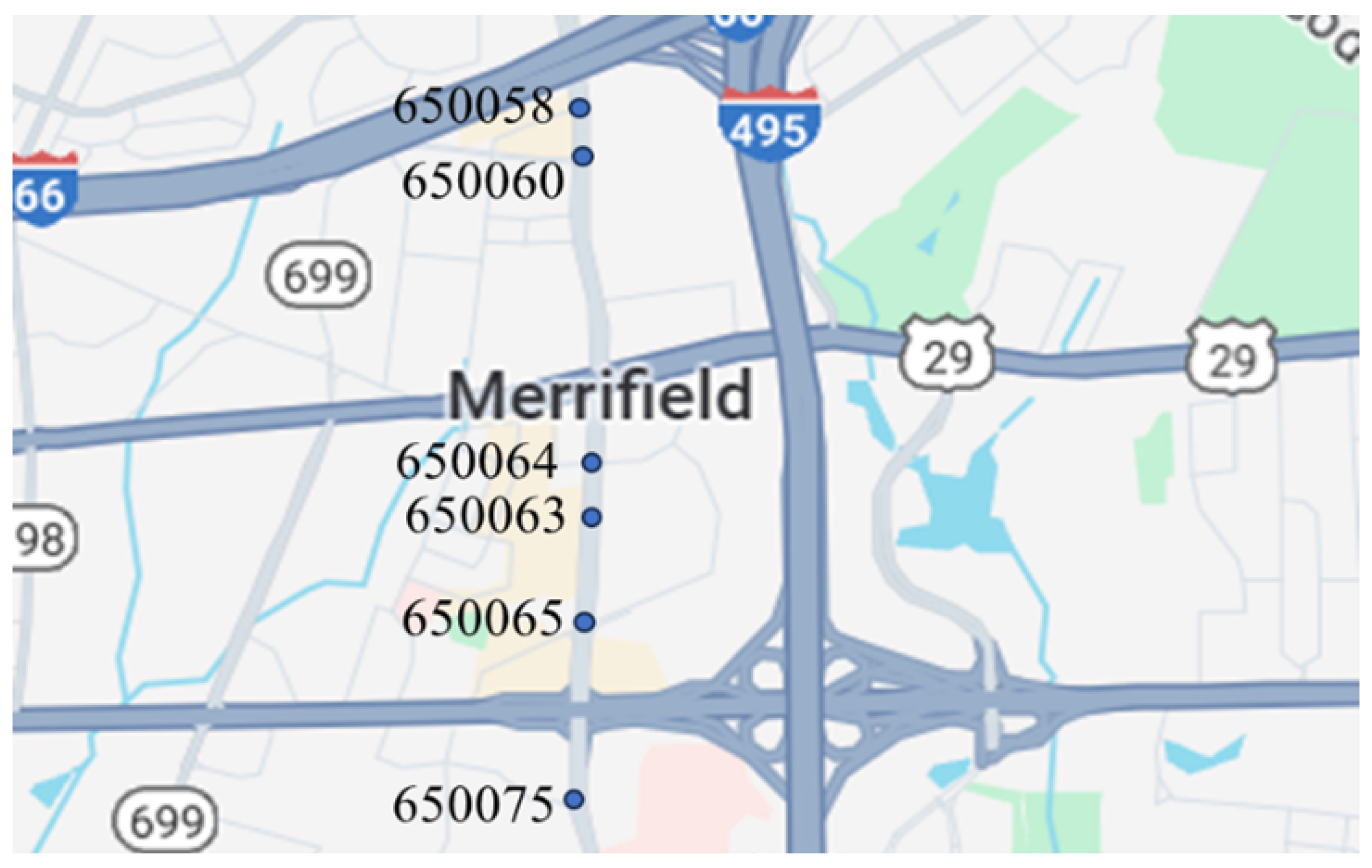
Figure 2.
Different variables in SmarterRoads data.
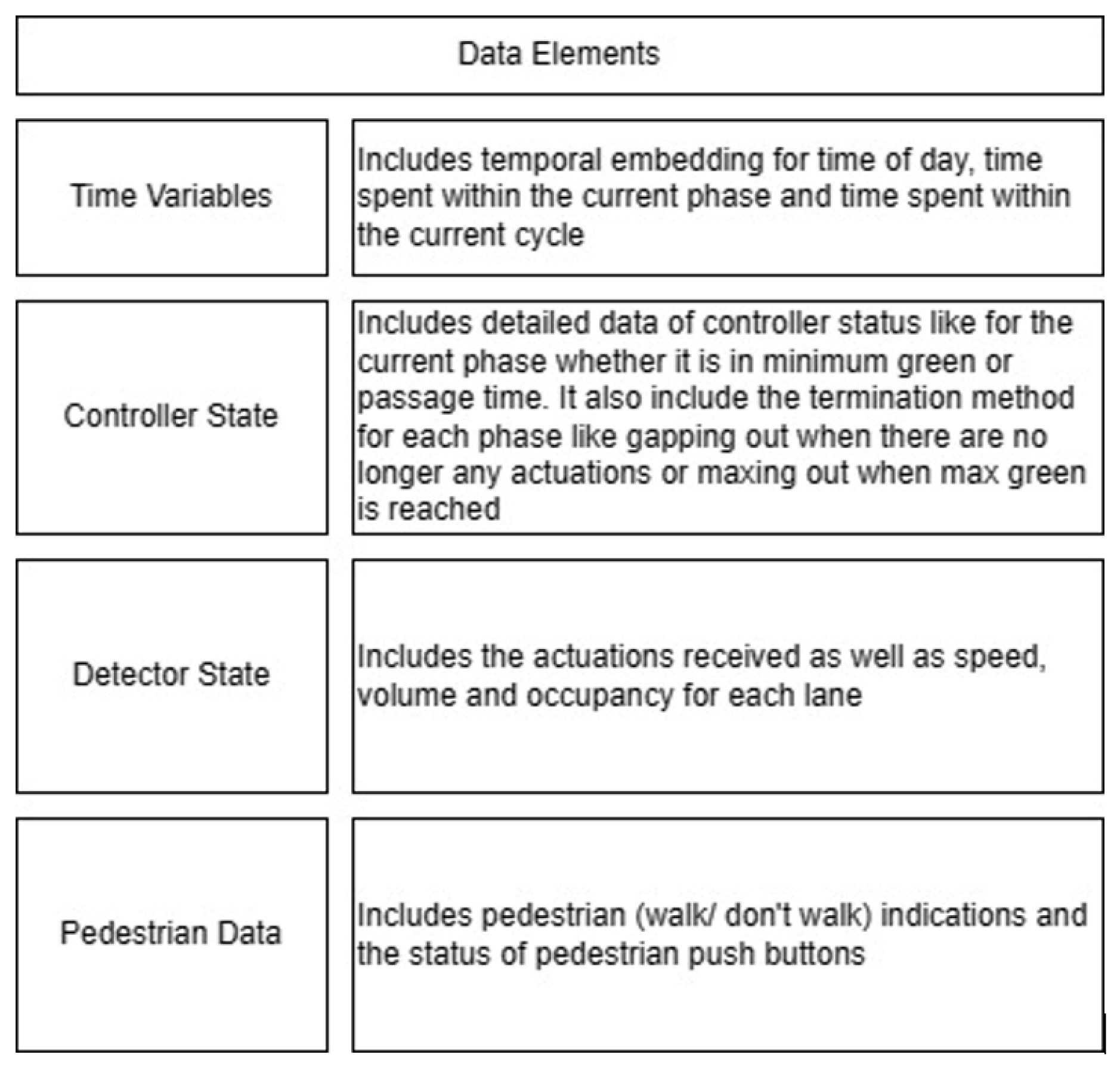
Table 1.
Phasing schemes for all 6 intersections studied.
Disclaimer/Publisher’s Note: The statements, opinions and data contained in all publications are solely those of the individual author(s) and contributor(s) and not of MDPI and/or the editor(s). MDPI and/or the editor(s) disclaim responsibility for any injury to people or property resulting from any ideas, methods, instructions or products referred to in the content. |
© 2025 by the authors. Licensee MDPI, Basel, Switzerland. This article is an open access article distributed under the terms and conditions of the Creative Commons Attribution (CC BY) license (http://creativecommons.org/licenses/by/4.0/).
Copyright: This open access article is published under a Creative Commons CC BY 4.0 license, which permit the free download, distribution, and reuse, provided that the author and preprint are cited in any reuse.


