Special Zero Gravity Theory

Francisco Javier Cuesta Gutierrez

doi:10.20944/preprints202501.1106.v1

Submitted:

05 January 2025

Posted:

14 January 2025

You are already at the latest version

Abstract

This paper has been renamed as “Special Zero Gravity Theory” because it preceds to another one called “General Zero Gravity Theory” of a different scope. A Theory strictly deduced from Einstein’s General Relativity Theory [1] is introduced in this paper. This Theory is also based in the premise “Gravity is an expression of the state of balance reached by matter in space-time” (from Artificial BioIntelligence Theory [5] by this same author, Amazon November 2023). Its mathematicals basis are deduced from [1] and exposed in detail. We prove that speed in its different forms (translation or rotation) is able to counteract the concavity created by the Gravity, creating at last instance a “Zero Gravity” effect. The relation between such effect with speed and altitude is shown through different sample graphs. We discuss the conditions that must be fulfilled for appying the theory in the case of spinning objects, showing some graphs for different altitudes, rotation speeds and diameters of objects (disks). Although such theoretical objects are supposed to have all their mass concentrated in their periphery, an “equivalent radius”(Re) is calculated for an object with shape of compact disc. The way for extrapolating Re to any kind of objects with other shapes is shown. The “partial Zero Gravity effect” is also calculated, showing that a partial effect can be reached for different speeds and altitudes. We also discuss the relation among the Zero Gravity effect and the energy conservation principle, between gravitational potential energy and kinetic energy. Finally we show the relation with the metric tensor of Einstein.

Keywords:

relativity gravity

;

space-time

;

Einstein tensor rotation speed

Subject:

Physical Sciences - Theoretical Physics

FOUNDATIONS OF THE THEORY

This study analyzes the possibility of avoiding the gravitational effect corresponding to Newton's Law of Universal Gravitation [3] when navigating in the vicinity of any celestial body, from the points closest to its surface, where such effect is greatest, to the most far away, where the influence is increasingly less.

To do this, we start from a strict interpretation of the Theory of Relativity [1], supported by the Theory of Artificial Biointelligence [5] of this same author, through which it is deduced that all celestial bodies are in a state of balance in the Universe, which is only altered when some “foreign body” to the system penetrates the “dent” of space-time in which said celestial body is immersed in its state of equilibrium in accordance with Einstein's Theory.

As a consequence, I consider that it should never again be stated that there is a gravitational force that attracts bodies, despite the fact that the simplification of the Theory of Relativity in Newton's Theory of Gravitation is more than sufficient to explain the interactions between nearby masses and to carry out the pertinent calculations when the intervention of the Time coordinate is not considered.

The real explanation of the phenomenon is that, when a body “falls” into the “dent” of space-time caused by another body, it is forced to “slide” into said dent, as happens with a marble when it falls into a hole. The effect may resemble that of the application of a force (“gravitational force”), so it can be explained with Newton's Theory, but the interpretation of the phenomenon is not correct.

It's about giving Time the authentic role it has in the Universe, which is none other than that of being one more axis of the coordinate system, but which at the same time maintains dependencies with the other three axes X, Y, Z of space, or in other words, it is not independent of them and therefore it’s not immutable.

The best way to understand a system of four coordinates X,Y,Z,t is to reduce it to a system of three coordinates, that is, to assume that the Universe was an X,Y plane where third coordinate (usually named as Z) was in this case time t.

Then we can imagine the distortion caused in time by a mass M that was located in an X,Y plane:

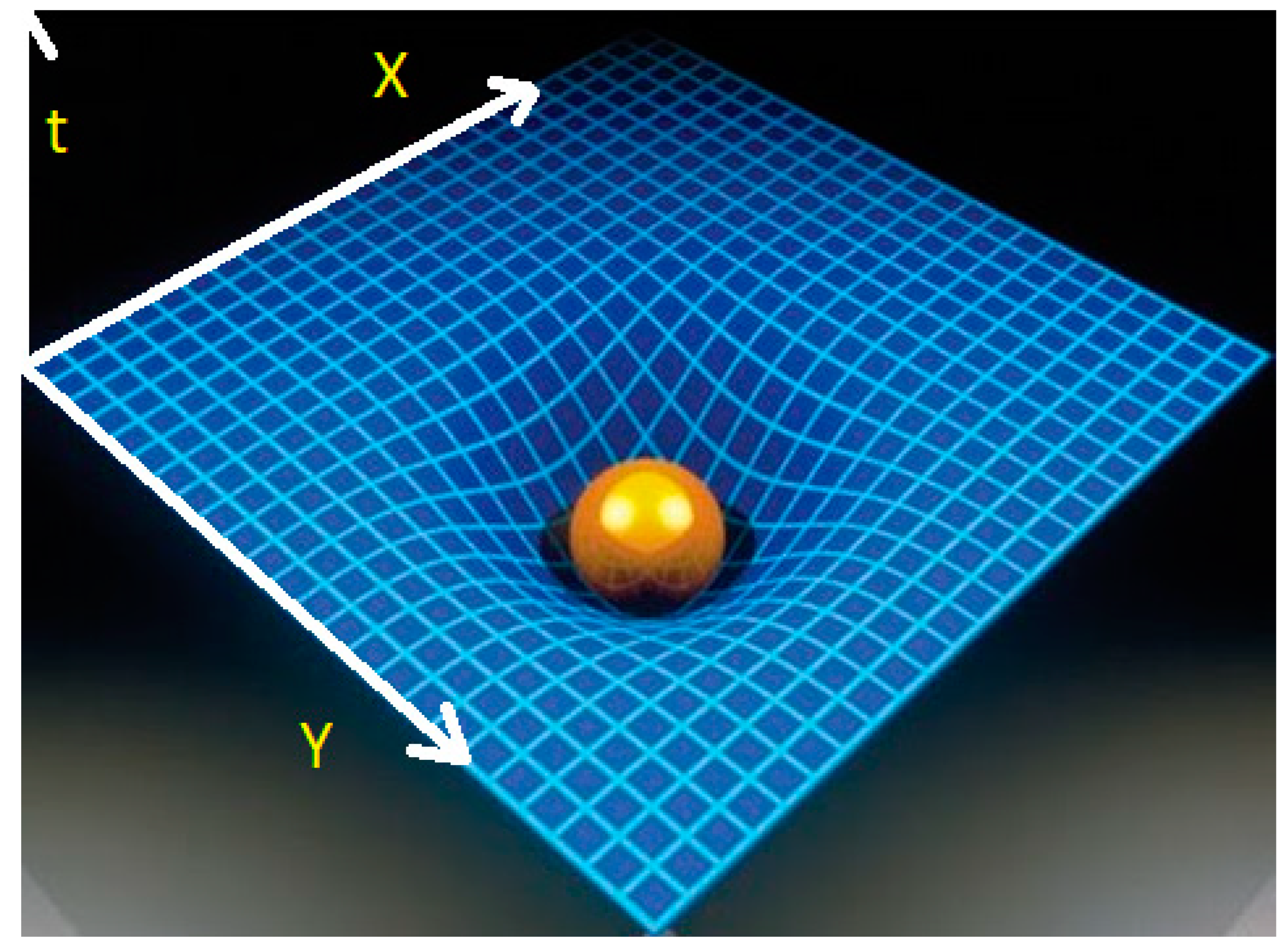
In this case, to simplify, the mass M is identified with the Earth, but obviously the reasoning would be the same for any celestial body.

DEVELOPMENT OF THE THEORY

According to the Theory of Relativity, time passes more slowly on the surface of the Earth and gradually faster as we move further into space.

Given that the mass of the Earth with respect to the magnitudes we are dealing with is small, the time differences are minimal (so much so that they are measured in nanoseconds), but the truth is that it can be stated, roughly speaking (since the reference should really be the center of gravity of the Earth), that for an inhabitant who lives in the mountains, time will pass faster than for someone who lives at sea level, that is, the higher the altitude, the faster they "age". Although we are exaggerating, since the differences are absolutely negligible for human beings.

The effect of “gravitation” on time, that is, the effect derived from the presence of a mass in its equilibrium state on space-time over any mass found in its environment, can be expressed through the Theory of General Relativity [1] and the Schwarzschild metric [4]. The time component of the metric tensor is

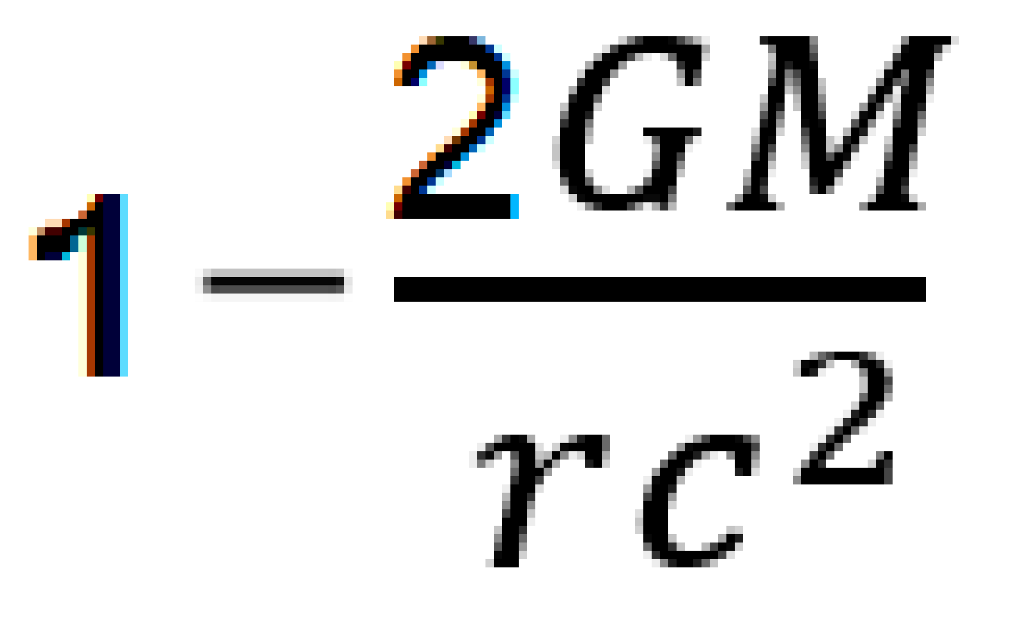
g00 =

Therefore the times difference can be expressed as

(T s - T e)

²

= Δ T s ² = \frac{2 G M}{r c^{2}} - \frac{2 G M}{(r + h) c^{2}}

(I)

Being h the distance between the sea level surface and the point S where we are at a height difference h above sea level, c is the speed of light, r is the radius of the Earth (6,371 km= 6,371 x 106 m.) G is universal constant=6.67 x 10-¹¹ Nm²/kg² and M the mass of the Earth (5.974 × 1024 Kg.

Now, if we assume that the object located at point S is traveling at a speed v, the Theory of Special Relativity [1] tells us on the other hand that there is a variation of time as a function of its speed. The formula in which the time difference is expressed is determined by the Lorentz Factor [2]:

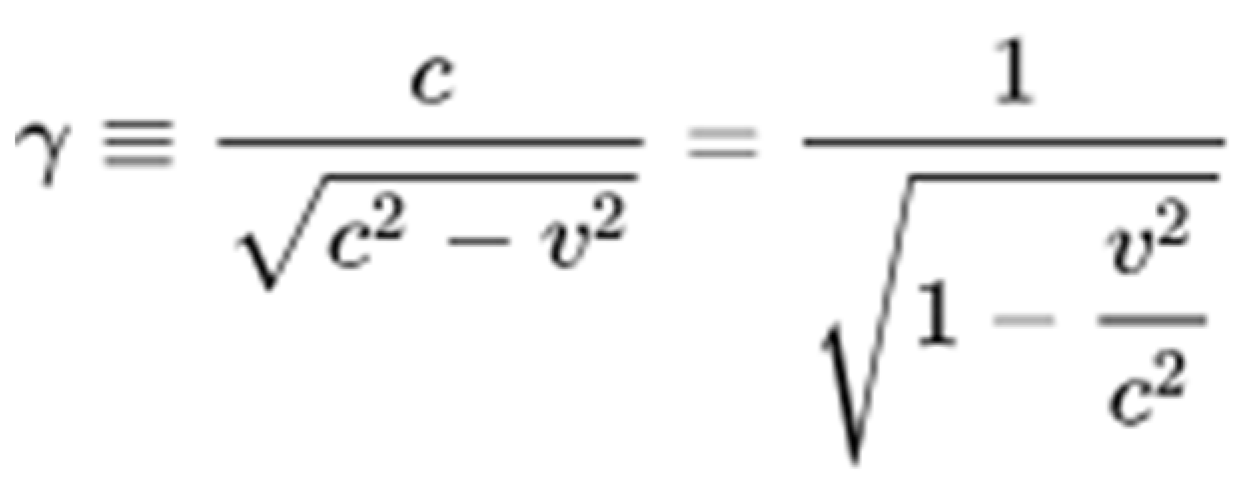
Being v the speed of an object at point S and c is the speed of Light.

The relation of times between an observer stationary on the surface of the Earth (Te) and another moving at a speed v at point S (Ts) will be the following:

Te=Ts.ϒ

That is, if we tend to the limit, so that v was equal to the speed of Light (v=c): then Te=∞

And expressed as a function of Te:

Ts=Te.1/ ϒ

Which can be expressed by homogeneity of times as

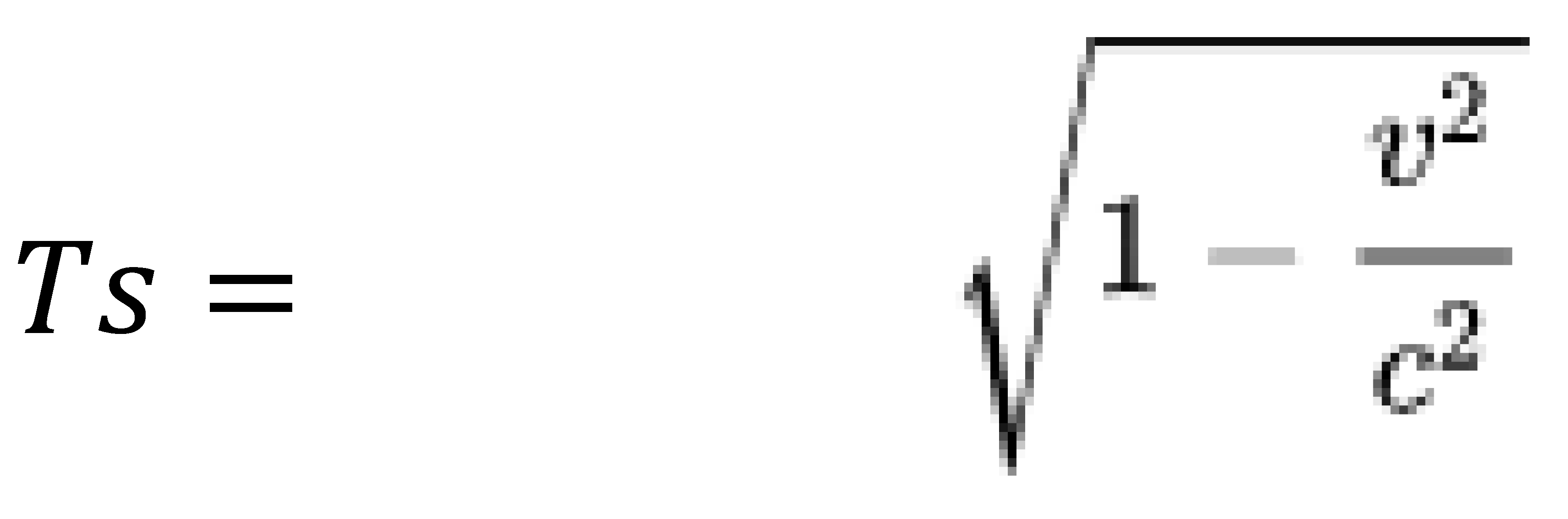
Then, for an object at point S traveling at the speed of Light, time would have stopped for an observer on Earth, in other words: at higher speeds, time passes more slowly, to the point that if the speed approached at the speed of light, for an insignificant time for the traveler at point S, it would turn out that an almost infinite time would have passed on Earth (if it still existed by then).

Therefore the times difference between an object traveling at speed v and at static state can be expressed as

Δ T s ²

=

\frac{v^{2}}{c^{2}}

(II)

There is a third relativistic phenomenon that should be taken into account, the so-called “Lense-Thirring effect”, which is generated by the angular momentum of the rotating mass M (in this case the Earth), which produces a “drag” effect over space time. You could say that it “drags” any “foreign object” to move in the direction of rotation. In the following image we illustrate it by exaggerating the phenomenon for a better interpretation:

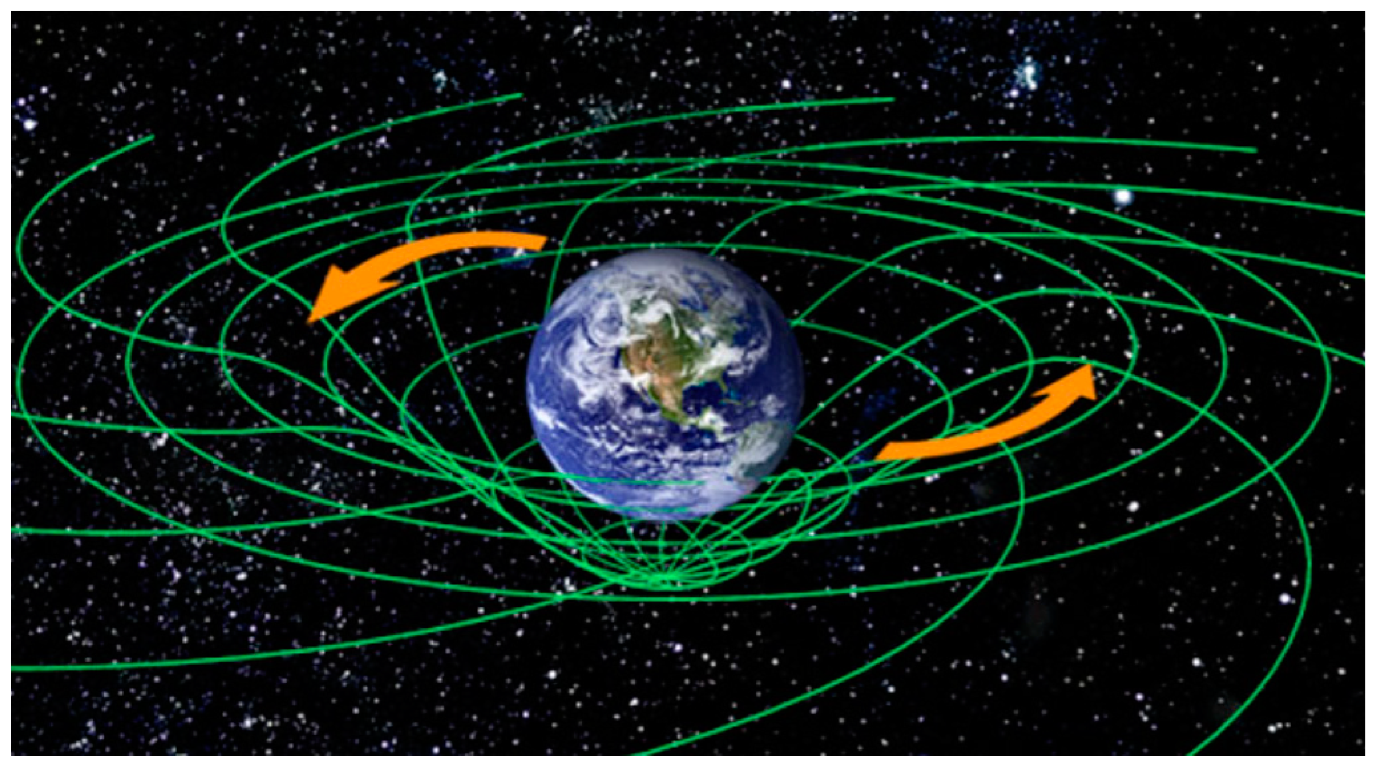
This effect, from a mathematical point of view, can be assimilated to that of a vortex in the Coriolis effect, which is why the formulas that define it are so similar. These are differential equations of the second degree, which would significantly complicate the calculations.

Therefore, we are going to ignore the “Lense-Thirring” effect in this discussion, since, in any case, its influence should not be quantitatively significant (probably less than 1%), especially at high altitudes.

This effect could be more or less important in other celestial bodies depending on their rotation speed (and obviously their masses), compared to that of the Earth.

There is a fourth relativistic phenomenon, called geodesic or de Sitter, related to a very small angle at which the Earth deforms its space-time. Its relevance is even much smaller than that of “Lense-Thirring” (probably around 10% of the previous one), so it is practically imperceptible.

In summary, for a traveler at a point S at a height h above the surface of the Earth moving at a speed v, there are two opposite time variations (this fact also happens, for example, with GPS satellites, so in that case proceeds to make a time correction):

The height h causes time at point S to pass faster than on Earth, according to formula (I)

The speed v of the traveler at point S causes time at that point to pass slower than on Earth, according to formula (II)

As we saw previously, it is the “dent” that is caused in the “mesh” of space-time by the presence of a mass M, or in other words, the deformation in t axis caused by said mass (when any object tries to alter its state of stability) the cause of the effect that colloquially, since Newton's time, we call “gravity”. But... what if we managed to alter that dent, in the sense of "flattening" it and making it non-existent?... In that case, if the dent for practical purposes "did not exist", no object would "fall" into it. What would happen is that the state of stability of the mass M would not be altered, since it would be “as if it had not even noticed” the presence of another object.

To achieve this effect, we must equalize the times expressed in formulas (I) and (II).

Making (I)=(II):

\frac{2 G M}{r c^{2}} - \frac{2 G M}{(r + h) c^{2}}

=

\frac{v^{2}}{c^{2}}

→

G M (\frac{1}{r} - \frac{1}{r + h}) = \frac{v^{2}}{2}

(**)

That is, v=

\sqrt 2 G M (\frac{1}{r} - \frac{1}{r + h})

(*)

Some examples:

For h=100 m. → v=44.32 m/s (159,55 Km/h)

For h=1000 m → v=140.15 m/s (504.55 Km/h)

For h=10000 m → v=442.89 m/s (1594.40 Km/h)

For h=30000 m → v=765.91 m/s (2757.27 Km/h)

For h=50000 m → v=987.24 m/s (3554.07 Km/h)

IMPORTANT: To make as few calculation errors as possible, values of constants such as G,M, r must be adopted with the highest possible resolution.

On the other hand, it must be taken into account that the values will be slightly modified depending on the longitude/latitude in which we find ourselves, since the simplification assumes that the Earth is perfectly spherical and its composition perfectly homogeneous, something that is obviously not true.

An improved version should take into account these circumstances, as well as the previously mentioned Lense-Thirring effect or, in maximum optimization, also the Sitter effect.

At the same time, we do not take into account the minimum deformation that the mass m presents in its space-time over that of the Earth, taking into account the enormous difference in the mass ratio.

However, for this exposition it is considered that the percentage difference in the error when dispensing with the previous effects would not be significant.

For impatients that can’t wait to know why we take the surface of Earth as reference, I suggest jump to the chapter about the singularity in the Theory where I think it’s clearly explained.

The theoretical final result is that a ship at a speed v and a height h resulting from (*) will “defy gravity” and travel under the “practical” effect of not being subjected to it (“zero gravity speed”).

And, vice versa, from (**), that is, from the equality of the equations (I)=(II), one can also calculate the height h at which one must travel at a speed v to get the “practical” effect of “zero gravity”.

For a ship that decides to travel continuously in “zero gravity”, such speed will have to be continually recalculated in real time by the onboard computer in order to adapt it to different altitudes.

It's attached the code of a simple Python program to calculate the speed of a ship as a function of altitude to travel in “zero gravity”.

Their values are shown in the diagram that follows the code:

#Zero Gravity

from scipy import constants

from math import sqrt

import numpy as np

#G=Gravitational Constant Newton

G=constants.G

speeds=[]

heights=[]

import matplotlib.pyplot as plt

import numpy as np

#R=Earth Radius (m.)

#M=Mass of Earth

R=6371000

m1=5.974

m2=10**24

M=m1*m2

h=0

k=sqrt(2*G*M)

for h in range (100,50000,100):

r1=1/R

r2=1/(R+h)

v=k*sqrt(r1-r2)

vkm=int(3.6*v)

heights.append(h)

speeds.append(vkm)

print("h, Speed (m/s),m(Km/h.)=",h,v,vkm)

# Draw points

plt.scatter(x = np.array(speeds), y = np.array(heights))

# Save graph in png format

plt.savefig('zerogravity.png')

# Show graph

plt.show()

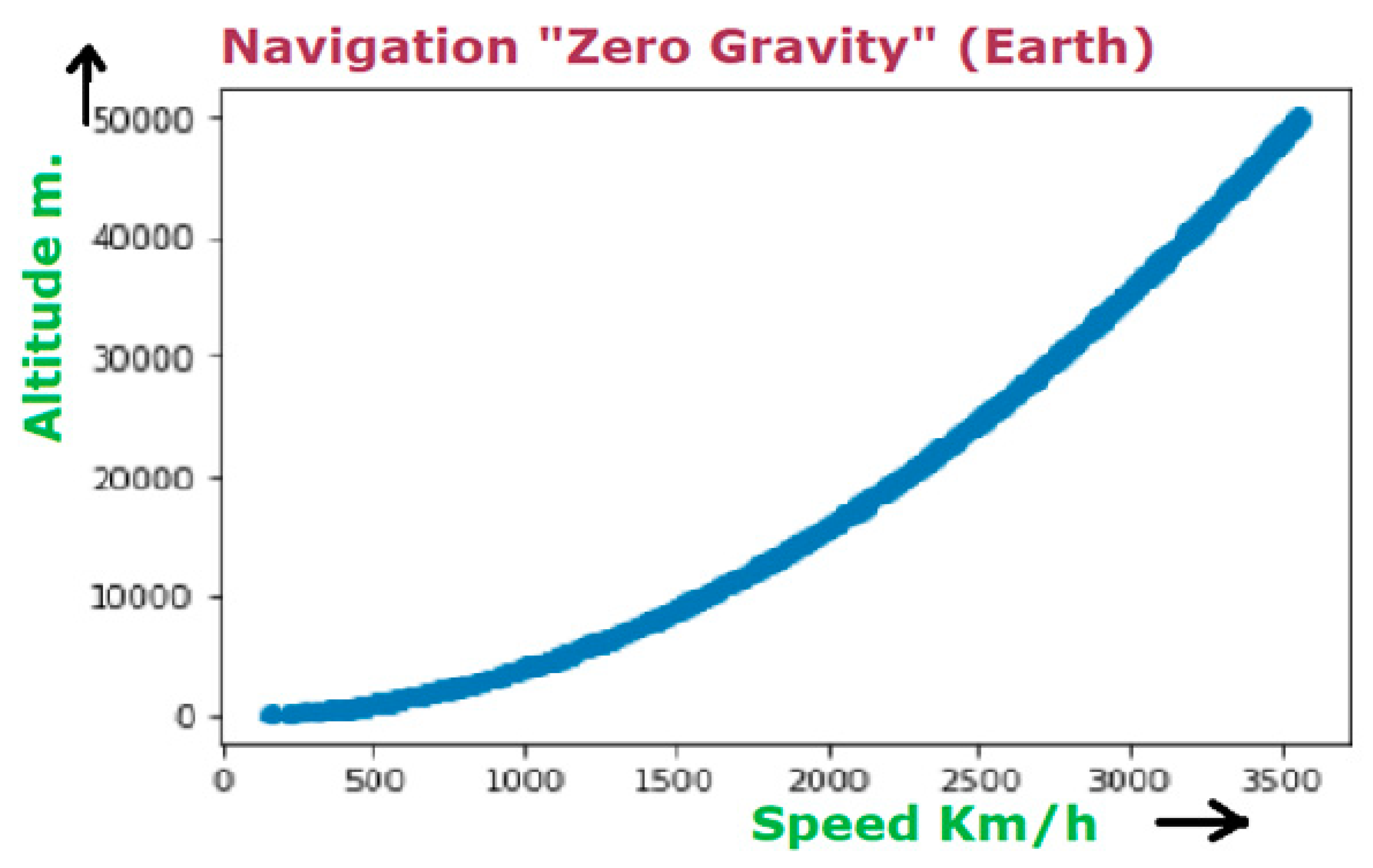
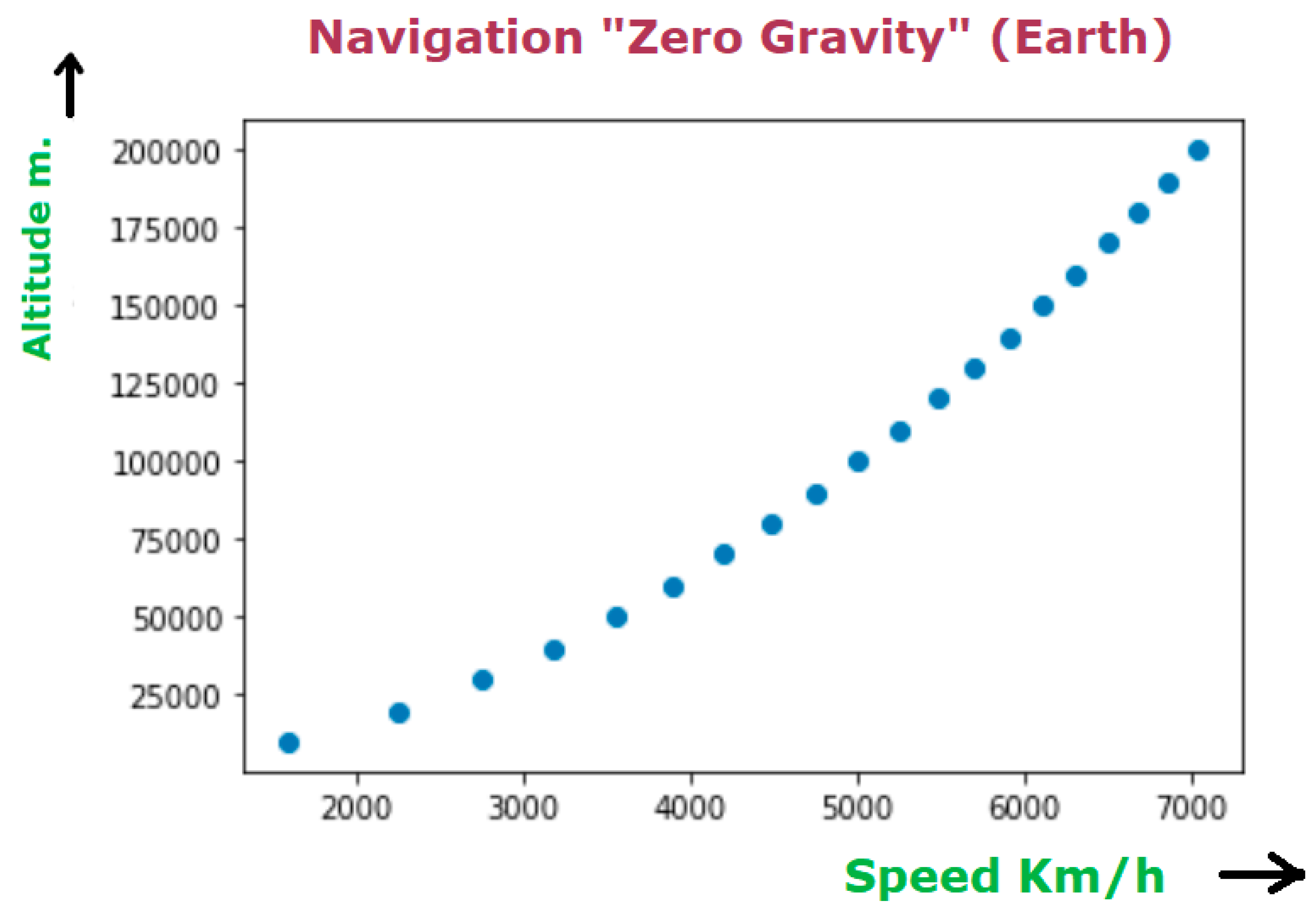
Or, if we expand to altitudes of up to 200 km:

Or, expanding to very high altitudes (80,000 km):

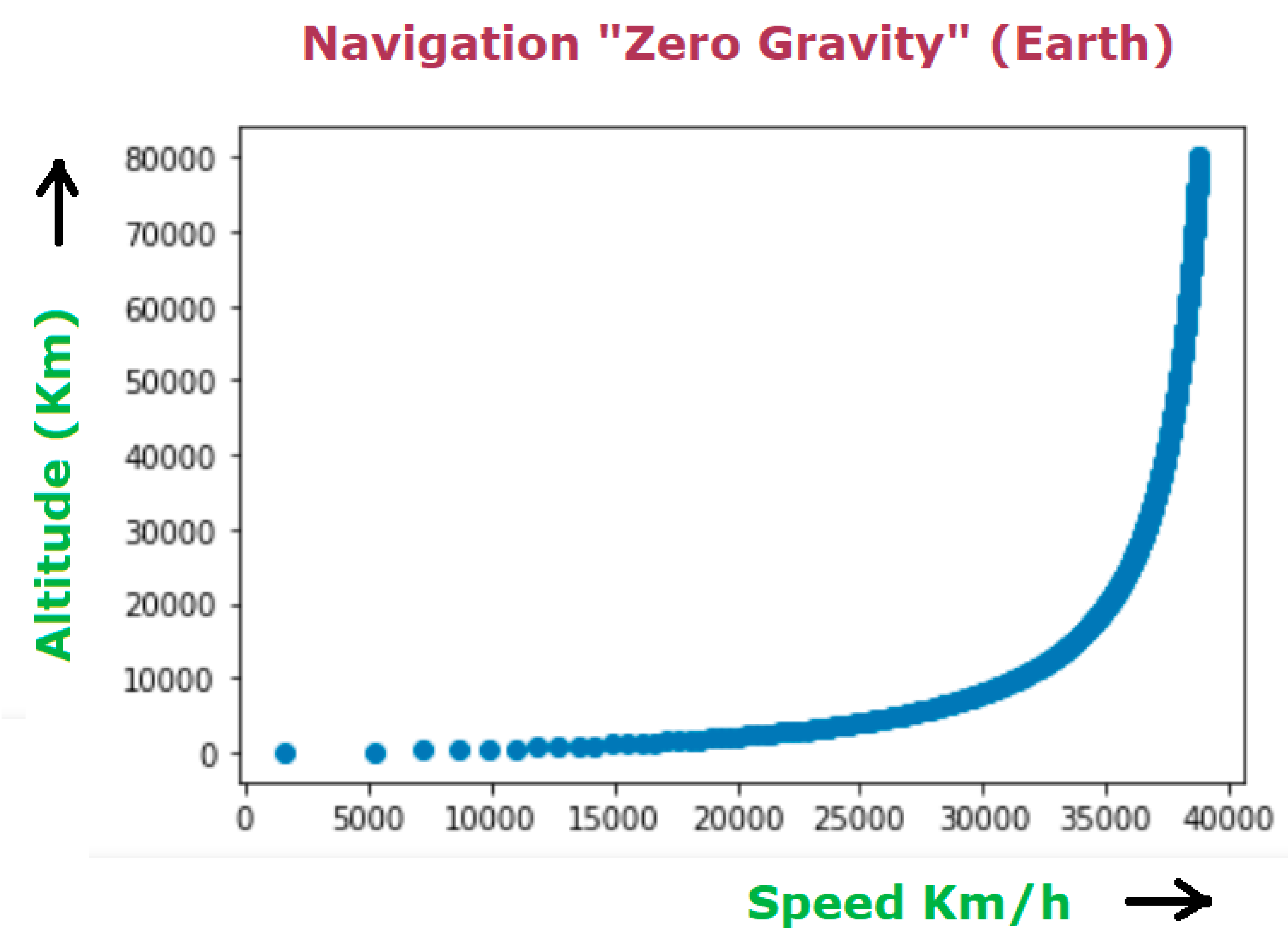
In this third graph we observe how, for high altitudes, where the effect of gravity is smaller, the curve tends to an asymptote close to 40,000 km/h, which matches with the “classical Newtonian” calculation value of the escape velocity. The physical reason is the greater the gravitational potential field, the greater the speed needed to counteract it. We’ll see this in detail in other chapter, when we talk about the partial zero gravity effect.

In turn, this third graph, in which at a certain height the speed of “zero gravity” matches with the classic escape speed, shows us the validity of this Theory.

This model has been applied to the Earth, but it is valid for any point in the Universe. With the exposed model, we should be able to navigate through space without that our ship being affected (once the corresponding calculations have been carried out in real time adapted to the environment where we are) by the “gravitational effect”, with the consequent drastic reduction of necessary energy.

It should also be an effective method to launch satellites into orbit simply and economically or to take any space ship into space (regardless of its size and weight) without increasing its inclination angle or the energy needed.

Finally, we should point out that, given that for each altitude there is a specific speed of “zero gravity”, the corresponding set of points (Vz,h), where Vz would be the “speed for zero gravity at altitude h”, would correspond to singular points for Newton's Theory, that is, they could seem not being affected by it.

As a consequence, it would be essential to make them known, so that air or land vehicles try not to approach the singular speed corresponding to the height they are in, since the consequences of entering, even for an insignificant amount of time, in “zero gravity” could be dangerous, even disastrous sometimes.

In the case of land vehicles (especially at low altitudes, close to sea level) there could be a momentary loss of grip, which if it coincided with a curved section or adverse weather conditions could cause a loss of control, until now attributed to other causes.

In the case of aerial vehicles, a sudden loss of height could occur, which in most cases would be assimilated to that of conventional turbulence, but in others it could lead to large losses of height until now inexplicable.

The “Lense-Thirring effect”, mentioned previously, could fundamentally cause a slight distortion of the speeds that we have calculated in two aspects:

Quantitatively, it would be more significant the closer we were to sea level, even more so taking into account that the “zero gravity speeds” corresponding to such altitudes are lower.
Qualitatively it would add or subtract depending on whether we were moving in the direction of the Earth's rotation or the opposite one.

Under these circumstances, what we have been looking for is getting to “flatten” the space-time so that the object/ship goes practically “unnoticed” by the Earth, “counteracting” the effects of a curved space.

Then we could ask ourselves if it would be possible not only to “flatten it”, but rather manage to move from the “concavity” of space-time to a convexity, that is, that the ship was “expedited” from the vicinity of the Earth.

This case would require a more detailed and exhaustive analysis, but in first instance we consider that we would be faced with a case in which, simply, the speed of the ship would be higher for each altitude than the corresponding singularity speed. Therefore the “convexity” would be the result, talking in conventional terms, of speed being able to “overcome” gravitational effects (without taking into account aerodynamic considerations).

In the event that we were able to prove the possibility of convexities in space-time by objects in movement, I consider that we could extrapolate as conclusion the possible existence of convexities in a general way in space-time and, in particular, to that of “white holes” which would “expel” mass (instead of “absorbing” it) given their extreme convexity (contrary to the extreme concavity of black holes).

White holes could therefore be found associated with “wormholes” or Einstein-Rosen bridges.

A SINGULARITY IN THE THEORY

This theory presents a singularity at sea level as reflected in the formula (*), when h=0.

This singularity is interpreted as due to the fact that the Theory is closely linked to the gravitational potential field, being the surface of the celestial body (the Earth in this case) our reference/origin which is also the origin of our Time axis.

We’ll explain forward in detail the close relationship among gravitational potential energy and kinetic energy and deduce how the principle of conservation of Energy is the key for understanding how Zero Gravity effect works. That is, although this Theory is coherent with different valid physical approaches, perhaps the energy balance is the best way of understanding the need of taking the surface as reference point and therefore such origin becomes a singularity.

APPLICATION TO ROTATING OBJECTS

Since the Theory of General Relativity was born there has been, and continues to be, a strong controversy regarding whether the rotation of an object in space follows relativistic or absolute guidelines. In other words: whether the rotation of an object should be considered absolute, that is, independent of the observer or not.

There are hypotheses in both senses. The main reason in favor of the absolutism of movement is that, according to the Theory of General Relativity, the speed is always relative to the reference system in question but the acceleration is always absolute. Since the rotation of an object around an axis of symmetry requires an acceleration that acts perpendicular to the tangential movement, that is, in the direction of the axis, called centripetal acceleration, said movement should be considered absolute. However, there are other hypotheses that consider that, despite this circumstance, uniform motion produced with a constant velocity should be considered relative, like any other linear motion.

For the case at hand, which is none other than the application of this Theory, the first rotating objects that would occur to us are probably those with a rotating axis perpendicular to sea level. Although it could be the subject of a simple experiment (simply applying rotation speeds as a function of altitude and diameter as we will indicate later), I consider that in this case, since the Z axis of the observer (which coincides with that of the "acceleration of gravity", g vector) and the axis of rotation are practically parallel, we would be closer to the "absolutist" case than to the "relativist" case.

However, I consider that the formulas that follow are perfectly applicable to any axis as long as the following critical technical considerations are respected:

1) Space crafts whose axis of rotation are strictly parallel to g, will not work. Some “excentricity” should be added (“spinning top effect”) although it’s not necessary that it’s ostensible. A little effect is enough, because the important fact is altering slightly (but continuously) the direction of the axis of rotation to be a relativistic one.

2)Space crafts whose rotation edge has another direction of rotation could also have the previous issue being the solution the same that the exposed in the previous point.

Taking into account the previous considerations, the present theory is also perfectly applicable to objects that are rotating around an axis of symmetry, either remaining practically immobile or simultaneously moving (which would obviously complicate the calculations).

The above formulas could also be applied to new models of rotating air and space ships, which could require a high rotation speed for high altitudes, depending in turn on their diameter.

Such rotation speed could be combined with the translation speed to achieve the desired function.

Although the “Lense-Thirring” effect should also be taken into account for high rotation speeds, we could obtain the following graphs for different diameters of the ship rotating around a symmetry axis by applying the same simplified formulas dividing the speed by the length of the circle (*):

(*) Assuming that all the mass is concentrated in the periphery, in the plane perpendicular to the axis of symmetry.

A model for different mass distributions is proposed later in this chapter

In previous graphs, the speed of rotation is expressed in Hertz (Hz), that is, the number of rotations (turns, revolutions) per second.

As can be seen, for a ship diameter of e.g. 50 meters, the ranges of the rotation speed to reach a state of “immobility” (or, although the name is not correct, “ingravity”) go from just over zero to 2.5 revolutions per second (0 to 10,000 meters altitude). However, for a “prototype ship” of only 10 cm. of diameter, ranges are among more than 100 and 1400 revolutions per second.

It should be emphasized that, as a direct consequence of the Theory, the necessary turning speed does not depend at all on the “weight” (it would be more correct to say “mass”) of the ship.

The axis of rotation could be any as long as it’s an axis of symmetry of the object.

Now, as mentioned above, these results are based on the premise that all the mass is concentrated in the periphery, that is, around the outer circle. Let's imagine that instead it is a solid disk, of radius R and homogeneous density rotating at an angular speed Ψ.

In this case, and at the expense of its evaluation through experimentation, we are going to propose a possible method.

This method is based on the concept of calculating an equivalent radius (Re), that is, a radius for which the “zero gravity” rotation speed is, for a solid disk of radius R, the same as that necessary for a disk of radius Re but with all its mass concentrated on its periphery.

To do this, taking into account the implication of both mass and speed, we are going to base our calculation on the mass x speed moment, equating that of the disk in its entirely with that of the theoretical disk of radius Re and mass theoretically arranged on its periphery.

Vx= X / R * Vr

dm= 2π X * dx

Equating with the momentum of an equivalent disk of radius Re:

That is, the Equivalent Radius Re for a solid disk would be Re= 2/3 R.

Also for more complex cases, in which the volume was based on the rotation of a polyline around an axis or on any surface capable of being defined through parametric coordinates or even with areas of different densities, it would be relatively simple to find the equivalent radius according to the formulas previously proposed.

In any case, this add on hypothesis that I propose for different types of geometry must obviously be experimented. So corresponding corrections can be made based on the results obtained.

If according to this Theory it is possible to “flatten” the space-time, it should also be possible to create a “convexity” in it.

To do this, by increasing the “equilibrium” or “weightlessness” rotation speed, the ship should be able to ascend. It would be the opposite effect of “gravitation”, so we could colloquially call it “anti-gravitation” (*).

In short, at speeds lower than the equilibrium rotation speed the gravitational effect (at different degrees, so we call it zero partial gravity) would prevail, at higher speeds the “anti-gravitational” effect would prevail.

It must be taken into account that the “equilibrium speed” is a function of the altitude, therefore it should need to be continually recalculated.

(*) Note: My experiments show that indeed the antigravity effect could be reached with a speed of rotation higher than the balance speed for zero gravity.

It’s also necessary to remember that we are using simplified formulas and that for a higher level of optimization the “Lense-Thirring” effect of the object should be also taken into account.

As a curious fact, if we relied only on rotation and not translation, to maintain “weightless” a ship of about 50 m. of diameter at high altitudes above the Earth, we would require a rotation speed of about 68 Hz. Logically, if the ship also moved simultaneously, the necessary rotation speed would decrease.

Therefore, new ships could be designed based on this Theory and not only on aerodynamics, not only for traveling to space but for transporting passengers and merchandise at the planet level.

Of the multiple designs that could emerge, there is one in particular that could powerfully capture attention: the one that has usually been called “flying saucer”, but we could also talk about spherical, cylindrical ships or with any surface definable by parametric coordinates.

In other words: not only similar to the classic views of UFOs but even other unimaginable ones, especially taking into account that in the case of air ships they could be combined with aerodynamics.

What there is no doubt is that they will bear little resemblance to conventional ones.

Significant fuel savings could also be achieved and even renewable energy could be used, because of their design geometry would not be forced to follow conventional aerodynamic rules.

ZERO GRAVITY PARTIAL EFFECT

In previous chapters we analyzed at what speed (linear and/or angular), an object at a certain altitude h would result in “flattening” space-time and, therefore, traveling under the effect of “zero gravity”.

We also wondered what would happen if the object traveled at a speed lower than the theoretical speed of “zero gravity” and, even, if at a speed higher than that of “zero gravity” the opposite effect could be achieved, that is, that the object object could be “repelled” instead of “attracted” by Gravity.

We are going to analyze the simplest case of both of them, that is, what happens when the object travels at a speed lower than that of “zero gravity”.

Our target is to find the relationship between speed and the gradual decrease in gravity associated with it (that is, the Partial Zero Gravity effect) until reaching the “full Zero Gravity” effect.

To do this, we are going to start from the time balance formula calculated in a previous chapter, based on which we deduced the speed of “Zero Gravity”:

\frac{G M}{r c^{2}} - \frac{G M}{(r + h) c^{2}}

=

\frac{v^{2}}{2 c^{2}}

→

G M (\frac{1}{r} - \frac{1}{r + h}) = \frac{v^{2}}{2}

(3)

If we now wanted to calculate the speed at which half of the time difference due to Gravity would be “compensated”, instead of completely compensating it, we would only have to divide the expression to the left of the equality by two, that is:

\frac{1}{2} * [G M (\frac{1}{r} - \frac{1}{r + h})] = \frac{v^{2}}{2}

from which we would solve the value of v.

And, in a general way, calling Xt the time differential factor (in the previous example 2), we can calculate the theoretical speeds at which we would compensate 1/Xt the time difference due to Gravity:

\frac{1}{X t} * [G M (\frac{1}{r} - \frac{1}{r + h})] = \frac{v^{2}}{2}

(4)

Therefore:

v=

\sqrt 2 G M (\frac{1}{r} - \frac{1}{r + h})

/

\sqrt X t

If we take the “zero gravity speed” (Vz) as a reference:

V=Vz/

\sqrt X t

Examples:

For Xt=1 → V=Vz

For Xt=2 → V=Vz/

\sqrt 2

For Xt=3 → V=Vz/

\sqrt 3

For Xt=4 → V=Vz/

\sqrt{4} = V z / 2

.

For Xt=10 → V=Vz/

\sqrt{10}

Another way of interpreting equation (3) is that it expresses the degree of conversion of gravitational potential energy into kinetic energy per unit of mass. The smaller Xt is, the greater its conversion, until it is complete for Xt=1.

When this conversion of gravitational potential energy into kinetic energy is completed, the “Zero Gravitation” effect is achieved for a given altitude. In other words: it is a consequence of the principle of conservation of energy.

This relationship between gravitational potential energy and kinetic energy explains that, the higher the altitude, the more speed (higher kinetic energy) is necessary to achieve the effect.

Furthermore, this relationship is implicitly reflected in Einstein's mathematical development that led him to affirm that the metric tensor (limited in this case to the component of times g00), which defines the simplified space-time for the Newtonian field, is the gravitational potential field (U).

Let's now see what it means to “compensate by speed” in 1/Xt the time difference due to Gravity:

Based on the equation (3) and the equation of difference of gravities

Δ

g among a point at the surface and at and altitude h:

Δ

g=

G M (\frac{1}{r^{2}} - \frac{1}{{(r + h)}^{2}})

(5)

Working a little bit both equations (3) and (5) we can reach to the following expression:

Δ

g =

Δ

Ts²

(\frac{1}{r} + \frac{1}{(r + h)}) \frac{c^{2}}{2}

(6)

That can be also expressed in function of speed v as

Δ

g =

\frac{v^{2}}{2} (\frac{1}{r} + \frac{1}{(r + h)})

(6b)

(6) and (6b) express (for any specific value of h) a linear relationship among

Δ

g and

Δ

Ts² and among

Δ

g and v².

Now it’s time to reflect this physical fact in a geometric symbolic simplification.

For doing this, we’re going to return to the starting point of this Theory of Zero Gravity. If we simplify the “deformation” effect produced by the mass on the Time axis (that is, without resorting to Einstein field equations), we could associate the conventional Gravity effect to a vertical line, the “Zero Gravity” effect to a horizontal line and the “Gravity with 1/Xt deformation” effect related with the Time axis to an oblique line.

NOTE.- The symbolic

Δ

t is really

Δ

Ts²

Figure 1. Analysis of the real gravity gr as a simplified function of the theoretical g and the time differences.

Being gr=g.cos(θ), the following values of gr as a function of Xt result:

Xt	θ	gr	V

1	90	0 g	Vz (*)
1.25	78.46	0.2 g	$V = Vz / \sqrt 1.25$
1.50	70.55	0.3 g	$V = Vz / \sqrt 1.5$
2	60	0.5 g	$V = Vz / \sqrt 2$
3	48.19	0.6667 g	$V = Vz / \sqrt 3$
4	41.41	0.75 g	$V = Vz / \sqrt 4$
5	36.87	0.80 g	$V = Vz / \sqrt 5$
6	33.90	0.83 g	$V = Vz / \sqrt 6$
7	31.02	0.857 g	$V = Vz / \sqrt 7$
8	28.96	0.875 g	$V = Vz / \sqrt 8$
9	27.38	0.888 g	$V = Vz / \sqrt 9$
10	25.84	0.9 g	$V = Vz / \sqrt 10$
15	21.09	0.933 g	$V = Vz / \sqrt 15$
20	18.19	0.95 g	$V = Vz / \sqrt 20$

(*) Horizontal position, V=Vz, xt=1, Ɵ=90, gr=0, “zero gravity” effect.

“Vertical position” for V=0, xt=∞, Ɵ=0, gr=g (vertical position).

NOTE.- The angle θ in this case is assumed to be “positive” in the clockwise direction, consistent with concavities in space-time.

RELEVANT CONSIDERATIONS

This theory is valid for objects in translation or rotation, as we discussed in previous chapters, with the following exceptions (just as previously mentioned):

1) It is not valid for objects either in free fall or that follow in any case the direction of the Gravity vector g, because they share the same reference system and relativity of times therefore makes no sense.

2) It is not valid, by analogous reasoning, for objects/ships whose axis of rotation fits with the direction of the Gravity vector g, since the centripetal acceleration could be considered absolute instead of relative in this case.

In these cases, such ships would have to perform, simultaneously with the rotation around their axis, an oscillatory type movement around it (colloquially speaking, “spinning top type”) to ensure that the movement could be considered relativistic and the considerations related to this Theory can therefore be applied.

3) For other axis of rotation, it is suggested that they have a slight eccentricity to prevent the acceleration vectors from continually maintaining a fixed angle.

However, in these cases it is relatively easy for the axis to have a small enough eccentricity to ensure that the rotation movement is relativistic.

Below we present graphs of speeds as a function of Xt and Gr for different altitudes achieved with a simple Python program.

We remember that the values for very low altitudes, close to the singularity (zero altitude) may present a relatively high margin of error.

Considerations for speeds higher than “Zero Gravity” speed:

From the formula (*) and Figure 1, it can be deduced that for values of xt < 1, that is, for speeds higher to “zero gravity speed” the object/ship could be theoretically “repelled” by the gravitational field.

It is obvious that this hypothesis has complete and coherent mathematical support. But it would be necessary to confirm whether it also has it in the physical sense, since we would be talking about accepting the possibility of achieving convexity in space-time based on the speed of an object.

In my modest opinion, convexities in space-time are as feasible as concavities (many times achieved through rotation), and in the particular case at hand, “negative effective gravity” could be totally feasible.

I omit the calculations due to their similarity to the previous ones and because I consider that this hypothesis should be especially checked and proven through experimentation.

PROOFS OF VALIDATION

Like any theory, this theory must be subjected to experimentation and testing, with the advantage that its verification is not too complex, and in fact I have allowed myself to carry out several tests, all successfully, with very simple equipment, which I will refer at the end of this chapter.

On the other hand, a few months ago some studies about of a strange magnetic levitation of causes not yet completely clarified appeared:

https://scitechdaily.com/defying-gravity-scientists-solve-mystery-of-magnetic-hovering-beyond-classical-physics/

In my opinion, the possibility that one of the magnets (the “floating magnet”) had reached the “zero gravity rotational speed” should be studied, which would help to explain partially the phenomenon. Especially taking into account that it is documented that the smaller the diameter of the “floating magnet”, the more speed of rotation is needed (which would be in line with everything previously stated).

Although experiment was done almost at sea level (Denmark) and therefore error margin could be high, the sizes of the floater magnets and the fact that levitation rotation speed is function of their diameters suggest that it’s likely that Zero Gravity could also be implied in the phenomena.

Therefore it would be interesting to repeat the same experiment at a higher altitude (more of 100 m.) to know if the results are exactly the same or not.

We would also suggest trying with larger magnets, not limiting the experiment to small objects.

In any case, it would also be important to take into account not only the size of the floating magnets, but also their shape, since this will influence the equilibrium rotation speed.

If the results at different altitudes were identical, the intervention of the “zero gravity” effect would have to be ruled out, but otherwise we would probably have the first proof of validity of the Theory, even prior to the experiments carried out on my part subsequently.

But the real proofs of this Theory have came from my own experimentation.

I have carried out some experiments.

Even though I do not have the most appropriate laboratory equipment and environment, I consider that the results are more than eloquent and prove the validity of the Theory.

The results (videos) can’t be obviously shown in this paper, but they’re published on my X profile, The reader can access to them at

https://x.com/jaimevoltius/status/1832821529274462396

All the updated information and the evidences as result of them can be found there.

References

Einstein, Albert (1920). Relativity. London,: Routledge. Edited by Robert W. Lawson.
Lorentz, H.A. (1904) Proceedings of the Royal Netherlands Academy of Arts and Sciences, 6, 809-831.
Newton, Isaac, 1642-1727. Newton's Principia : the Mathematical Principles of Natural Philosophy. New-York :Daniel Adee, 1846.
Karl Schwarzschild, “Uber das Gravitationsfeld einer Kugel aus inkom pressibler Flussigkeit nach der Einsteinschen Theorie”, Sitzungsberichte der K¨oniglich Preussischen Akademie der Wissenschaften, 1916 vol.
Cuesta, F.J. (2023) Theory of Artificial BioIntelligence. Amazon, November 2023.

Disclaimer/Publisher’s Note: The statements, opinions and data contained in all publications are solely those of the individual author(s) and contributor(s) and not of MDPI and/or the editor(s). MDPI and/or the editor(s) disclaim responsibility for any injury to people or property resulting from any ideas, methods, instructions or products referred to in the content.

© 2025 by the authors. Licensee MDPI, Basel, Switzerland. This article is an open access article distributed under the terms and conditions of the Creative Commons Attribution (CC BY) license (http://creativecommons.org/licenses/by/4.0/).

Copyright: This open access article is published under a Creative Commons CC BY 4.0 license, which permit the free download, distribution, and reuse, provided that the author and preprint are cited in any reuse.