Submitted:
09 January 2025
Posted:
14 January 2025
You are already at the latest version
Abstract
We propose a new supervised learning algorithm, where each data point in test set is included into the class into which such inclusion causes minimum displacement in the existing n-th central moment of the respective class under construction. After each such inclusion, the n-th central moment of the corresponding class is updated by some incremental calculations in constant time, i.e., each class evolves gradually and changes its definition incrementally after the inclusion of every new data point. We then use k-fold and stratified k-fold cross validation techniques to compare the performance of our proposed model with various state of the art supervised learning algorithms including Neural Network (NN), Support Vector Machine (SVM), Random Forest (RF), K-Nearest Neighbor (KNN) and Logistic Regression (LR) using Pima Indian Diabetes (PID) dataset, which is a popular dataset in machine learning research. Our analyses suggest that the performances of our proposed algorithms involving lower order moments are comparable to that of K-Nearest Neighbor (KNN) with a far better testing time complexity, while it is a bit under-performed as compared to Logistic Regression (LR), Support Vector Machine (SVM) and Random Forest (RF) in terms of accuracy. Our analyses also suggest that our proposed algorithms also outperform the Neural Network (NN) models with relatively lower number of nodes and layers. However, if we continue to increase nodes and layers in the Neural Network, it tends to outperform the proposed algorithm. In a nutshell, the performances of different MDEM algorithms as proposed here involving different order of moments vary within the range of [83.19%-95.82%] of the best algorithm under consideration in k-fold and stratified k-fold cross validation techniques.
Keywords:
supervised learning
; raw moments
; central moments
; time complexity
; cross validation
1. Introduction and Scope of the Current Study
To date, there are numerous supervised machine learning algorithms each having its own strength and weakness. For example, K-Nearest Neighbor (KNN), one of the earliest and perhaps most straightforward algorithm for supervised learning has the ability to train itself in constant time, i.e., as soon as a labelled input is provided, the model can learn it instantly without further processing. However, it has a testing complexity of , where n is the total number of training data, d is the dimensionality of the feature space. This is a rather daunting task, specifically when we have to deal with a large set of training data, as we need to calculate the distance between the new point and all other previously classified points ([1]). Using techniques like KD Tree and Ball Tree, average running time in the testing phase can be improved up to at the expense of a costlier time complexity in the training phase ([2,3]). However, the worst-case time complexity is still ([2,3]).
Apart from the KNN, another most studied supervised learning algorithm is Support Vector Machine (SVM) that aims to construct maximum margin hyperplanes amongst the training data points ([4]). The time complexity of SVM method depends, among other things, upon the algorithm used for optimization (e.g., quadratic programming or gradient-based methods), dimensionality of the data, the type of the kernel function used, number of support vectors, and the size of the training dataset. Worst-case time complexity in training phase of linear and non-linear SVMs are found to be and respectively, where T is the number of iterations, n is the size of the training sample and d is the dimensionality of the feature space ([5,6]). Time complexities of the testing phase of SVMs are found to be for linear kernel and for non-linear kernel, where s is the number of support vectors.
Another algorithm that is frequently used in classification of labelled data is Random Forest (RF), which is an ensemble learning technique that works by constructing multiple decision trees in the training phase, where each tree is trained with a subset of the total data ([7]). To predict the final output of the RF in testing phase, majority voting technique is used to combine the results of multiple decision trees. The time complexity of RF depends upon the number of trees in the forest (t), sample size (n), dimensionality of the feature space (d) and tree height (h) among other things. Training time complexity of RF is found to be , while the testing complexity is per sample.
Another important algorithm for classification is Logistic Regression (LR), which is used primarily for binary classification, although the algorithm can be easily adapted to handle multiclass classification problems as well. Training phase time complexity of the Logistic Regression (LR) depends, among others, on number of training samples, number of iterations and dimensionality of the features space, where the number of iterations depends further on the choice of the algorithm used (stochastic, batch gradient descent or, alike) ([8]). In a nutshell, the total time complexity of the Logistic Regression (LR) in training phase can be summarized as , where E is the number of iterations, n is the size of the training sample and d is the dimensionality of the input space. On the other hand, the testing time complexity of LR per sample is as it simply involves computing the dot product of the weight (w) and feature vector (x) ([8,9]).
However, perhaps one of the most popular and widely used supervised learning algorithms is the Neural Network (NN), which is inspired from the networks of biological neurons that comprise human brain and is presently used extensively in image and video processing, natural language processing, healthcare, autonomous vehicle routing, finance, robotics, gaming and entertainment, marketing and customer service, anomaly detection etc. Performance of a Neural Network (NN) depends upon the number of hidden layers, number of neurons per layer, number of epochs, input size, input dimensions etc. If there are L hidden layers each having M neurons, then the training time complexity of the Neural Network (NN) can be summarized as , where E is the number of epochs/iterations, n is the sample size and d is the dimensionality of the input space, while the testing time complexity per sample of the said NN is ([10,11]). Choices of the number of hidden layers L, number of neurons per layer M and number of epochs E are somewhat arbitrary, i.e., we can choose any value for and E from a seemingly infinite range.
In fact, all of the above algorithms apart from KNN have one or more arbitrary parameters to be set, e.g., number of iterations, number of trees, choice of optimization algorithm, choice of kernels, number of hidden layers, number of nodes in each hidden layer, choice of activation function etc. Although KNN has a deterministic training and testing complexity, which can be anticipated beforehand, its testing time complexity is linear on training space, which is a very time-consuming process and renders KNN effectively ineffective in case of large training data. Here, we propose a new supervised learning algorithm that has a deterministic running time and can learn in time and classify new inputs in times, where n is the number of inputs, d is the dimensionality of input space and k is the number of classes under consideration. For a specific problem, the dimensionality of input space d and the number of classes k are fixed. Thus, unlike KNN, the training phase time complexity of our proposed algorithm is linear on the number of inputs and the testing time complexity per sample is constant. So, whenever we need a light-weight deterministic algorithm like KNN that, unlike KNN, can effectively classify new instances in constant time, we can use our proposed algorithm, which does not involve solving a complex quadratic programming problem (as like SVM) or, operations that require matrix multiplication (for NN) or, the alike.
In the training phase, our proposed algorithm resorts to find the n-th moment (raw or central) of each attribute of every class. At testing phase, the algorithm temporarily includes the new input into each of the k classes and computes the new, temporary n-th moment for each attribute of each class resulting from such temporary inclusion. The new input will then be finally classified into the class for which such inclusion causes minimum displacement in the existing n-th moment of the underlying class attributes. Once the new input is classified, the n-th moment of the attributes of the respective class is updated to reflect the change, while the moments of all other classes are left unchanged. Thus, apart from classifying new input in constant time, our algorithm also evolves incrementally after inclusion of every new data point, which makes the model dynamic in nature.
The rest of the article is organized as follows: section: 2 provides the definitions of raw and central moments as used in our analysis, section: 3 provides the new algorithm for supervised learning based upon Minimum Displacement in Existing Moment (MDEM) technique as improvised here, section: 4 discusses the time complexities of the proposed algorithm, section: 5 presents the methodology used for empirical analysis, section: 6 describes and elaborates the data, section: 7 presents various preprocessing techniques used for data cleansing, section: 8 discusses the empirical results and compares the performance of our proposed algorithms to that of various state of the art supervised learning techniques including K-Nearest Neighbor (KNN), Support Vector Machine (SVM), Random Forest (RF), Logistic Regression (LR) and Neural Network (NN), and finally, section: 9 concludes the article.
2. Raw and Central Moments
2.1. Raw Moment
n-th Raw moment of a random variable X is defined as the expected value of the n-th power of X, i.e.,
When , the first raw moment of X is the mean of the random variable X.
2.2. Central moment
n-th central moment of a random variable X is defined as the expected value of the n-th power of the deviation of the random variable X from its mean. Mathematically,
When , the first central moment of the random variable X about its mean is zero and when , the second central moment is the variance of the random variable X. For any arbitrary n, if we extend the expression of using binomial theorem, we get the following expression:
Using the linearity property of the expectation operator, we can simplify Equation: 1 for as follows:
For , Equation: 1 can be simplified into the following form to get the 3rd central moment about the mean:
And for , Equation: 1 can be simplified as below to get the 4th central moment about the mean:
3. Proposed supervised learning algorithm based upon Minimum Displacement in Existing Moment (MDEM)
We begin our analysis by sketching the algorithm for the 1st raw moment, i.e., mean. In this step, we intuitively describe the main idea behind the current discourse and then in subsequent steps, we enhance the reasoning to account for higher order central moments of the classes under construction.
3.1. MDEM in Mean
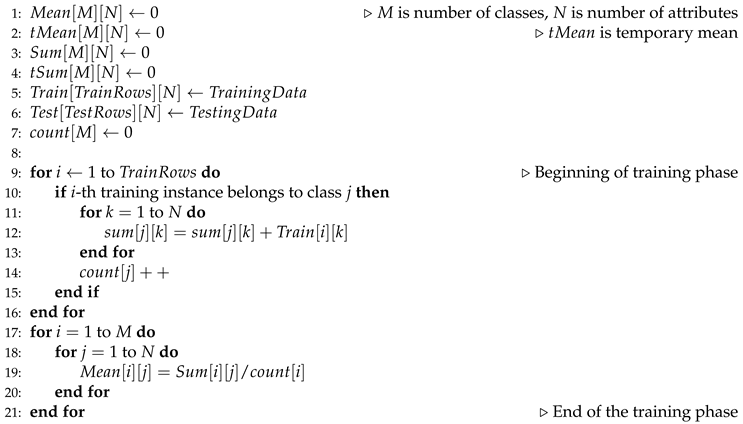
Let us assume that we are attempting to solve a multiclass classification problem involving M different classes. The classes are enumerated from 1 to M. Let us also assume that each of the training instances has N number of attributes. Based upon the value of these N attributes, each training instance is classified into one of the M possible classes. To begin with, we scan each of the training inputs one at a time and incrementally calculate the sum of the attributes of the respective class. Sum of the k-th attributes of all the training instances belonging to the j-th class is stored into . This is done through line of Algorithm: 1. As soon as a new training instance is found to belong to class j, the is increased by one. After we are done with scanning of the training rows, we calculate the mean of each attribute of every class. This is done simply by dividing the , by , . This is done in line of Algorithm: 1. This marks the end of the training phase of our algorithm.
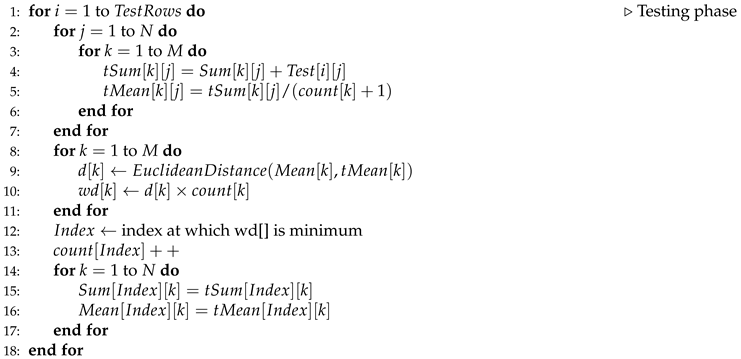
At the end of the training phase, we have an array of , which is a 2D array containing the mean of j-th attribute of i-th class at . We also have another 2D array, namely, containing the sum of all of the j-th attributes of the training instances belonging to i-th class at . In the testing phase, we incrementally enhance the as soon as a new instance is classified into class i by our proposed algorithm. Thus, after every increment, our algorithm evolves to accommodate the new changes. At the very beginning of the testing step, we scan a new test row and temporarily include it into every possible class. This will allow us to calculate the new temporary mean of every attribute of each class after such pseudo inclusion. This is done in line of Algorithm: 2. Next, we find the Euclidean distance between the existing mean and new temporary mean for each class. This is to be noted in this regard that both and , are N-dimensional vectors of the attributes. This is done in line of Algorithm: 2.
Euclidean distances thus calculated need to be multiplied by the cardinality of the respective class lest the class with high cardinality eat up every new point due to its gravitational pull. This is diagrammatically presented in Figure 1. In Figure 1, we have two classes, namely, Class-1 and Class-2. Class-1 already has 46 members in it, while Class-2 only has 2 members. As soon as we have a new point A to be classified, we notice that the inclusion of point A causes very little displacement in the existing mean of Class-1 as compared to Class-2. To be precise, inclusion of point A into Class-1 causes its mean (Class-1’s mean) to be shifted from point 1 to point 2. However, if point A is instead classified into Class-2, then its mean (Class-2’s mean) is shifted from point 3 to point 4. As evident from Figure 1, distance between is quite small as compared to that of . So, apparently at this point, we may consider the new point A to be classified into Class-1. However, as we can visually comprehend from Figure 1, point A is supposed to be classified into Class-2. To resolve the issue, we multiply the Euclidean distance calculated as above by the cardinality of the respective class. This modification of weighting the Euclidean distance by the class cardinality is done in line 10 of Algorithm: 2.
Next, we find the at which is minimized and this represents the class of this new testing instance under consideration. Then, we update the sum and mean of all attributes of class by the temporary sum and temporary mean respectively. All other means and sums (other than that of class) are left unchanged before the commencement of the new iteration with a new testing instance.
| Algorithm 1 Pseudocode for MDEM in mean: Training phase |
 |
| Algorithm 2 Pseudocode for MDEM in mean: Testing phase |
 |
3.2. MDEM in n-th central moment
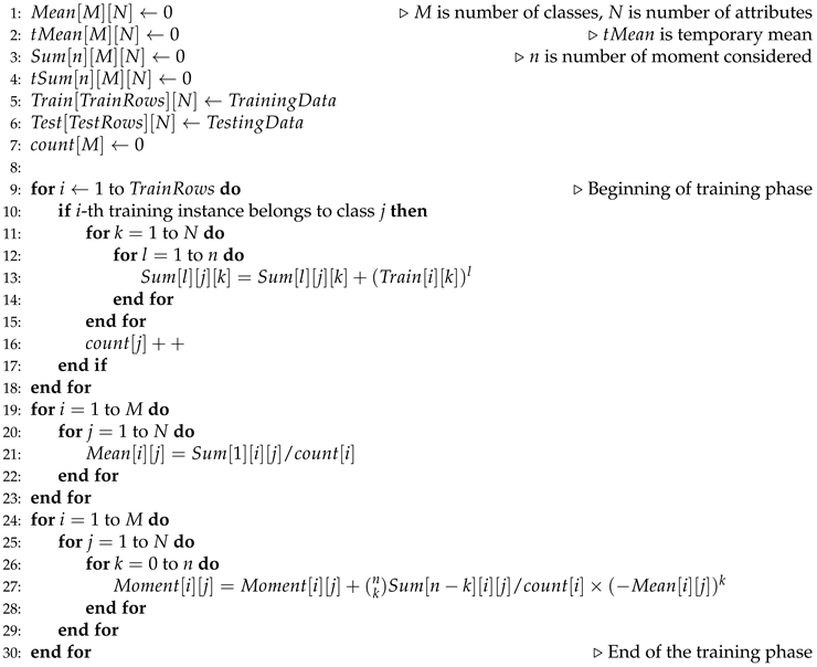
The proposed algorithm involving higher order central moments intuitively uses the same idea as discussed in the previous subsection. In the training phase, we calculate the mean and n-th central moment of every attribute of each class. Let us numerically describe the idea using 3rd order central moments (). Let us assume that the 5th attribute of the 2nd class has values of , which has a mean of . So, the 3rd central moment of the 5th attribute of the 2nd class is: or, . So, after the training phase, we have the mean and n-th central moment of each attribute of every class. At the testing phase, the new instance is temporarily included into all of the classes and the new temporary n-th central moment of each attribute of every class is calculated. Now, for each class , both the temporary n-th central moment and existing n-th central moments are vectors of length N, where N is the number attributes. Next, for each class j, we calculate the N-dimensional Euclidean distance between the temporary and existing n-th central moment. The distance thus calculated is then multiplied by the cardinality of the respective class in order to avoid the most densely populated class from engulfing every new test input.
To calculate n-th central moment in line with Equation: 1, we have to have the l-th powered sum () for each attribute of each class beforehand. These powered sums are generated in line of Algorithm: 3, where indicates l-th powered sum of the k-th attribute of the j-th class. Apart from the powered sums of each attribute of each class, we need to calculate the mean of each attribute of each class in order to determine n-th central moments for each attribute of each class in line with Equation: 1. These means are generated in line of Algorithm: 3. Once we have the means and powered sums, we can calculate the n-th central moments according to formula given in Equation: 1. To generate the expected values for any combination of n-th central moment and mean, we need to divide it by the cardinality of the respective class. The calculation of the n-th central moments are done in line of Algorithm: 3. This marks the end of the training phase of our algorithm.
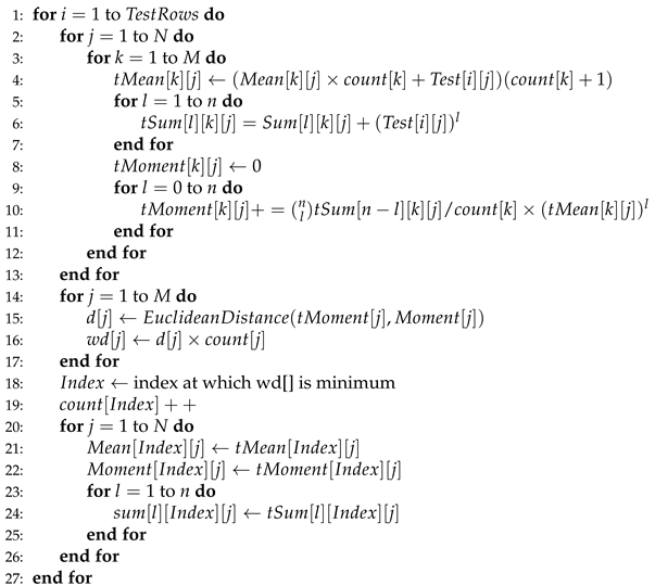
After the end of the training phase, we have captured the values of n-th central moment of the attribute () of i-th class () in . Next, we temporarily include every new testing instance into every possible class and calculate the new temporary moment of each attribute of each class resulting from such temporary inclusion. This is done in line of Algorithm: 4. Next, we calculate the N-dimensional Euclidean distance between the temporary and existing n-th central moments and weight each such distance by the respective cardinality of each class. This is done in line of Algorithm: 4 and these weighted distances are preserved in . Next, we select the index value at which the weighted distance is minimized and this index value indicates the class to which the new test instance is classified by our algorithm. Once the class is fixed for the new instance, the existing moments, means and powered sums corresponding to that specific class are set to the temporary moment, temporary mean and temporary powered sums as calculated previously and the count for that specific class in increased by one. These are done in line of Algorithm: 4. For all other classes, existing means, moments and powered sums are left unchanged before the beginning of a new iteration for yet-to-be-classified test rows.
4. Time Complexity Analysis of the MDEM Algorithm
In this section, we will analyze the time complexity of our proposed algorithm both in training and testing phase. We split our analysis into two parts: In first part, we determine the training and testing time complexity of MDEM in mean and in the second part, we analyze the training and testing time complexity of MDEM algorithms involving higher order central moments.
4.1. Time Complexity of MDEM in Mean
In the training phase, we scan the training rows one by one, check the class of each instance, and if the class value is found to be j, then the value of is increased by the amount of the k-th attribute value of the training instance under consideration. This is done in line of Algorithm: 1. So, time complexity of this step in the training phase is , where P is the number of training rows. As the number of attributes N for a specific problem is fixed, the overall time complexity of this step is linear on the number of training rows. Once we have calculated the for all the training rows, we can divide by , to get the mean value of each attribute of each class. This is done in line of Algorithm: 1. Time needed in this step is . For a specific problem, the number of classes (M) and the number of attributes (N) are fixed. Thus, the overall time complexity of the training phase is , where P is the number of training instances.
In the testing phase, we temporarily include each testing instance in every class and calculate the temporary mean of each attribute of each class, which can be done times, where M is the number of classes, N is the number of attributes. This is done in line of Algorithm: 2. Next, we calculate weighted and unweighted Euclidean distance between existing and temporary mean of each class, which is done in line of Algorithm: 2. Again, this can be done in time. Next, we find the index value at which the weighted Euclidean distance as calculated above is minimized, which is calculated in time (line 12 of Algorithm: 2). Finally, we update the sum and mean with the temporary sum and temporary mean of the attribute values of the respective class, which is done time (line of Algorithm: 2). For a specific problem, M and N are fixed, which implies, every new instance can be classified in constant time.
4.2. Time Complexity of MDEM in n-th Central Moment
In the training phase, we need to calculate n (n is the number of moments considered) number of powered sums as shown in line of Algorithm: 3. This can be done in times. This step of calculating the powered sums needs to be repeated for each of the N attributes of the training row under consideration. So, for each training row, we need to calculate powered sums (line of Algorithm: 3). Steps as mentioned in line are repeated for each training rows as well, and if there are P number of training rows, then we need number of operations in line of Algorithm: 3. For a specific problem, n and N are fixed beforehand. Thus, the time complexity of line of training phase is linear on number of training rows, i.e., . Once the powered sums are generated, we can calculate the mean of each attribute of each class in time (line of Algorithm: 3) and the n-th central moment of each attribute of each class in time (line of Algorithm: 3). As for a specific problem, the values of and N are prefixed, the overall time complexity of the training phase is linear on the number of training instances, i.e., .
At the testing phase, we temporarily include every test instance into each of the possible M classes and calculate the resulting temporary means, temporary powered sums and temporary moments (line of Algorithm: 4) of each attribute of every class. For every test row, we need to calculate the temporary mean (line 4 of Algorithm: 4), temporary powered sums (line of Algorithm: 4) and temporary moments (line of Algorithm: 4) for each attribute of each class, which can be calculated in , and time respectively. As for a specific problem, the values of and N are predetermined, the above steps can be completed in constant time for every new test instance. The next step in the testing phase involves calculating the weighted and unweighted Euclidean distance between the vectors of existing and temporary moments of every class (line of Algorithm: 4), which can be done in time. Finding the index value at which such weighted distance is minimum (line 18), can be done again in time. Finally, updating the mean, temporary moment and temporary powered sums for the respective class can be done in and time (line ). As we have mentioned previously, the values of and N are fixed beforehand for a specific problem, which implies that the overall time complexity of classifying a new testing instance is constant.
| Algorithm 3 Pseudocode for MDEM in n-th central moment: Training phase |
 |
| Algorithm 4 Pseudocode for MDEM in n-th central moment: Testing phase |
 |
5. Methodology
To begin with, we apply various data preprocessing techniques, e.g., identification and replacement of missing values, detection and removal of outliers using Inter Quartile Range (IQR) filter and feature scaling techniques to normalize the data within the range [0-1]. Processed data are then fed into various machine learning algorithms including MDEM in mean, MDEM in variance (2nd central moment), MDEM in 3rd central moment, MDEM in 4th central moment, KNN with 3, 5, 7 neighbors, Support Vector Machine (SVM), Logistic Regression (LR), Random Forest (RF) and Neural Network (NN) with 1, 2, 3 hidden layers each comprising 5 neurons with 50, 100 and 150 epochs. We use Equation: 2, 3 and 4 to calculate 2nd, 3rd and 4th central moments used in our proposed analysis based on Minimum Displacement in Existing Moment (MDEM) technique.
For the purpose of this analysis, we randomly split our dataset into k equally sized folds. We then use some folds to train our model and the rest 1 fold is used to analyze the performance of the trained model, which is popularly known as k-fold cross validation technique. The choice of k is rather arbitrary and there exists bias-variance trade-offs associated with the choice of k in k-fold cross validation ([12]). One of the preferred choices for k is 5, as it is shown to yield test error estimates that do not suffer either from excessively high bias or from extreme variances ([12]). So, we check the performance of different machine learning algorithms using 5-fold cross validation technique. Apart from that, we also compare the performance of different algorithms under 2, 3 and 7-fold cross validation also.
While k-Fold cross validation technique may perform well for balanced data, its performance deteriorates once it is used handle imbalanced or skewed data ([13]). As we will mention later in the data section, the data used in our present analysis are skewed to some degree, e.g., we have unequal number of observations in each class. To overcome the hurdles faced by k-fold cross validation techniques to classify imbalanced data, we use stratified k-fold cross validation, which intends to solve the problem of imbalanced data to some extent. In stratified k-fold cross validation, the folds are generated by preserving the relative percentage of each class. Like k-fold, we use 2, 3, 5 and 7 number of folds in our stratified k-fold cross validation technique to analyze the performance of different algorithms.
6. Description of Data
We collect Pima Indian Diabetes (PID) dataset originally developed by the National Institute of Diabetes and Digestive and Kidney Diseases (NIDDK), which is part of the United States’ National Institutes of Health. The Pima Indians are native American people, who traditionally lived along the Gila and Salt rivers in Arizona, United States and can now be found in various parts of Arizona, US and Mexico ([14]). This group has a high prevalence of diabetes among its members and diabetes research around the Pima Indians are often considered to be significant and representative of the global health ([15]). The PID dataset comprises records of some 768 females having age 21 and above from the Pima Indian population and is widely considered as a benchmark dataset in diabetes research ([16]). 08 (eight) attributes, namely, number of pregnancies, plasma glucose concentration in an oral glucose tolerance test, diastolic blood pressure, triceps skin fold thickness, serum insulin level, BMI, diabetes pedigree function, age and a class variable representing the prevalence of diabetes in the respective individual are recorded. Descriptive statistics of the PID dataset are presented in Table 1.
As can be seen from Table 1, out of 768 records in PID dataset, 500 are non-diabetic, while the rest 268 are diabetic.
7. Data Preprocessing
Data preprocessing is essential before feeding any data into machine learning algorithms as it helps build a better machine learning model with greater accuracy. Data preprocessing in our current analysis involves identification and replacement of missing values, detection and removal of the outliers and normalization.
7.1. Identification and Replacement of Missing Values
In this step, we identify the missing values in the PID dataset and replace them with the corresponding mean values. It has been observed that three attributes, namely, number of pregnancies, diabetes pedigree function and age have no missing values, i.e., we have all 768 values for these three attributes. For the other attributes, there are some missing values. To be precise, plasma glucose level, blood pressure, triceps skin thickness, insulin level and BMI have 5, 35, 227, 374 and 11 missing values. We replace the missing values with their respective mean values for the sake of our current analysis.
7.2. Detection and Removal of Outliers
In this step, we identify and remove outliers from the PID dataset. Outliers are simply data points that differ significantly from all other data points under consideration and they may arise due to variability in the measurement, experimental errors etc. So, in this step, we remove the outliers from the dataset lest we run the risk of building an over-fitted model that may perform well for training data but, behaves poorly for new test data. We use Inter Quartile Range (IQR) filter to detect and remove outliers from our dataset. After applying the IQR filter on our data, we have observed that there are 49 outliers and 719 normal records. We remove these 49 outliers from our analysis and continue with the remaining 719 observations.
7.3. Feature Scaling
Feature scaling is a data preprocessing technique intended to standardize the attribute values within a permissible range. In our present analysis, we have heterogeneous attribute values that differ significantly from one another in their orders of magnitude. For example, the number of pregnancies in our sample data varies between [0-17], while data on plasma glucose level swings between an even larger range of [44-199]. So, if we do not normalize the data, then the machine learning algorithms will tend to provide higher weightages to plasma glucose level than number of pregnancies, which is not intended. Thus, by normalizing all the attribute values within the range [0-1], we can build a better machine learning model. We use unsupervised normalization filter in Weka to normalize the attribute values within the range of [0-1].
8. Results
We run 19 different machine learning algorithms, namely, MDEM (in 4 variants), Logistic Regression (LR), Random Forest (RF), Support Vector Machine (SVM), K-Nearest Neighbor (KNN) (in 3 variants), Neural Network (NN) (in 9 variants) and note down their performances based upon their ability to properly classify PID dataset. Results obtained in our analyses are presented in Table 2 and Table 3. Table 2 documents the performance of different algorithms under 2, 3, 5, 7-fold cross validation technique, while Table 3 records the same for stratified 2, 3, 5, 7-fold cross validation. From Table 2, we can see that MDEM in mean, variance, 3rd and 4th central moment have obtained accuracy scores of , , and respectively under 2-fold cross validation technique. The accuracies obtained by Logistic Regression (LR), Random Forest (RF) and Support Vector Machine (SVM) are found to be , and . On the other hand, KNN algorithms with 3, 5, 7 neighbors have accuracies of , and respectively. Moreover, the performance of the NN varies somewhere between to depending upon the number of hidden layers and epochs. Best for the NN under current consideration, i.e., accuracy score of is obtained for NN with 3 hidden layers with 150 epochs, while the worst is obtained for NN with 1 hidden layer in 100 epochs. As can be seen from Table 2, MDEM in mean runs better than KNN with 3, 5, 7 neighbors and 8 (eight) out of NN models under consideration in 2-fold cross validation technique. The best algorithm under 2-fold cross validation is found to be Support Vector Machine (SVM) having a run time accuracy of . So, the performances of MDEM in 04 different variants are within the range of of the best algorithm under consideration. The results are graphically presented in Figure 2.
Under 3-fold cross validation, the accuracies of MDEM in mean, variance, 3rd and 4th central moments are , , and respectively. The best algorithm under 3-fold cross validation is Logistic Regression (LR) having an accuracy of . So, the performances of different variants of MDEM are within the range of of the best algorithm for 3-fold. Details are given in Figure 2.
For 5-fold cross validation, the accuracies of different MDEM algorithms are , , and respectively. As can be seen from Table 2, the best algorithm under 5-fold cross validation technique is identified to be Support Vector Machine (SVM) with a run time accuracy of . So, MDEM algorithms run within the range of of the best algorithm under 5-fold cross validation. Details are given in Figure 2.
For 7-fold cross validation, the accuracies of MDEM in mean, variance, 3rd and 4th central moments are , , and respectively. The best algorithm for 7-fold cross validation is found to be Support Vector Machine (SVM) with a run time accuracy of . So, different MDEM algorithms run within the range of of the best algorithm under 7-fold cross validation technique. Detailed results are graphically presented in Figure 2. To summarize, the performance of different MDEM algorithms varies between of the best algorithm under 2, 3, 5 and 7-Fold cross validation technique.
As we have mentioned earlier, there are 719 records after the outliers and extreme values are removed from our PID dataset. Out of these 719 records under consideration, 477 records are non-diabetic and 242 are diabetic. So, the sample under consideration is not quite uniform. Rather, it is skewed to some extent towards non-diabetic records. A preferred choice to work with such imbalanced dataset is to use stratified k-fold cross validation technique instead of simple k-fold. In this part of this analysis, we are going to summarize the performances of different MDEM algorithms along with other state of the art algorithms under stratified 2, 3, 5 and 7-fold cross validation techniques. The detailed results are presented into Table 3, while the summarized statistics are shown graphically in Figure 3.
From Table 3, we can see that the accuracies of MDEM algorithms in mean, variance, 3rd and 4th central moment under stratified 2-fold cross validation are , , and . The best algorithm in this case is found to be Logistic Regression (LR) with a run time accuracy of . So, MDEM algorithms run within the range of of the best algorithm under consideration. This is graphically presented in Figure 3.
Under stratified 3-fold cross validation technique, accuracies of different MDEM algorithms are found to be , , and , where MDEM in mean is the best performing one, while MDEM in 3rd central moment is the worst performing one with run time accuracy of and respectively. The best algorithm under stratified 3-fold cross validation is Logistic Regression (LR) with an accuracy of . So, as can be seen from Figure 3, different MDEM algorithms run within the range of of the best algorithm under consideration.
Moreover, the run time performances of different MDEM algorithms under stratified 5-fold cross validation technique are found to be , , and . The best algorithm under current scenario is Logistic Regression (LR) with an accuracy of . This implies, MDEM algorithms run within the range of of the best algorithm under present consideration as can be seen from Figure 3.
Finally, we analyze the performance of different algorithms under stratified 7-fold cross validation technique. As can be seen from Table 3, MDEM in mean, variance, 3rd and 4th central moment have accuracies of , , and respectively. The best algorithm under stratified 7-fold cross validation is Random Forest (RF) with a run time accuracy of . So, MDEM algorithms run within the range of of the best algorithm under consideration.
9. Conclusion and Future Work
Here, we have proposed a new supervised learning algorithm that can train itself in times linear to the number of training rows. After the training phase, the algorithm can effectively classify every new instance in constant time and can instantly change its definition after each such inclusion. As we have discussed throughout this article, this significant improvement in running time is obtained at the cost of a slightly less than optimal performance. For the Pima Indian Diabetes (PID) dataset, our algorithms are found to perform within the range of of the best algorithm at hand. Moreover, it has also been observed that MDEMs involving lower order moments can perform particularly better than their higher order counterparts for this specific problem. So, whenever we are in need of a multiclass classification algorithm that is intended to handle massive amount of input data, different variants of our proposed MDEM algorithms can come up as a suitable choice with a far better running time and a slightly less than optimal performance. However, before reaching any concrete decision regarding the usability of different MDEM algorithms, the proposed idea needs to be tested on a seemingly infinite number of multiclass classification problem, which is beyond the scope of the current study.
Funding
No funding is received to accomplish this work.
Conflicts of Interest
The author declares that no conflict of interest exists.
References
- Arya, S.; Mount, D.M.; Netanyahu, N.S.; Silverman, R.; Wu, A.Y. An optimal algorithm for approximate nearest neighbor searching fixed dimensions. Journal of the ACM (JACM) 1998, 45, 891–923. [Google Scholar] [CrossRef]
- Bentley, J.L. Multidimensional binary search trees used for associative searching. Communications of the ACM 1975, 18, 509–517. [Google Scholar] [CrossRef]
- Yianilos, P.N. Data structures and algorithms for nearest neighbor search in general metric spaces. In Proceedings of the Soda, Vol. 93; 1993; pp. 311–21. [Google Scholar]
- Cortes, C. Support-Vector Networks. Machine Learning 1995. [Google Scholar] [CrossRef]
- Burges, C.J. A tutorial on support vector machines for pattern recognition. Data mining and knowledge discovery 1998, 2, 121–167. [Google Scholar] [CrossRef]
- Chang, C.C.; Lin, C.J. LIBSVM: a library for support vector machines. ACM transactions on intelligent systems and technology (TIST) 2011, 2, 1–27. [Google Scholar] [CrossRef]
- Ho, T.K. Random decision forests. In Proceedings of the Proceedings of 3rd international conference on document analysis and recognition. IEEE, 1995, Vol. 1, pp. 278–282.
- Bishop, C.M.; Nasrabadi, N.M. Pattern recognition and machine learning; Vol. 4, Springer, 2006.
- Hosmer Jr, D.W.; Lemeshow, S.; Sturdivant, R.X. Applied logistic regression; John Wiley & Sons, 2013.
- Goodfellow, I. Deep learning, 2016.
- Bengio, Y. Learning Deep Architectures for AI, 2009.
- Gareth, J.; Daniela, W.; Trevor, H.; Robert, T. An introduction to statistical learning: with applications in R; Spinger, 2013.
- He, H.; Ma, Y. Imbalanced learning: foundations, algorithms, and applications 2013.
- Schulz, L.O.; Bennett, P.H.; Ravussin, E.; Kidd, J.R.; Kidd, K.K.; Esparza, J.; Valencia, M.E. Effects of traditional and western environments on prevalence of type 2 diabetes in Pima Indians in Mexico and the US. Diabetes care 2006, 29, 1866–1871. [Google Scholar] [CrossRef] [PubMed]
- Chang, V.; Bailey, J.; Xu, Q.A.; Sun, Z. Pima Indians diabetes mellitus classification based on machine learning (ML) algorithms. Neural Computing and Applications 2023, 35, 16157–16173. [Google Scholar] [CrossRef] [PubMed]
- Larabi-Marie-Sainte, S.; Aburahmah, L.; Almohaini, R.; Saba, T. Current techniques for diabetes prediction: review and case study. Applied Sciences 2019, 9, 4604. [Google Scholar] [CrossRef]
Figure 1.
Insertion of new data point
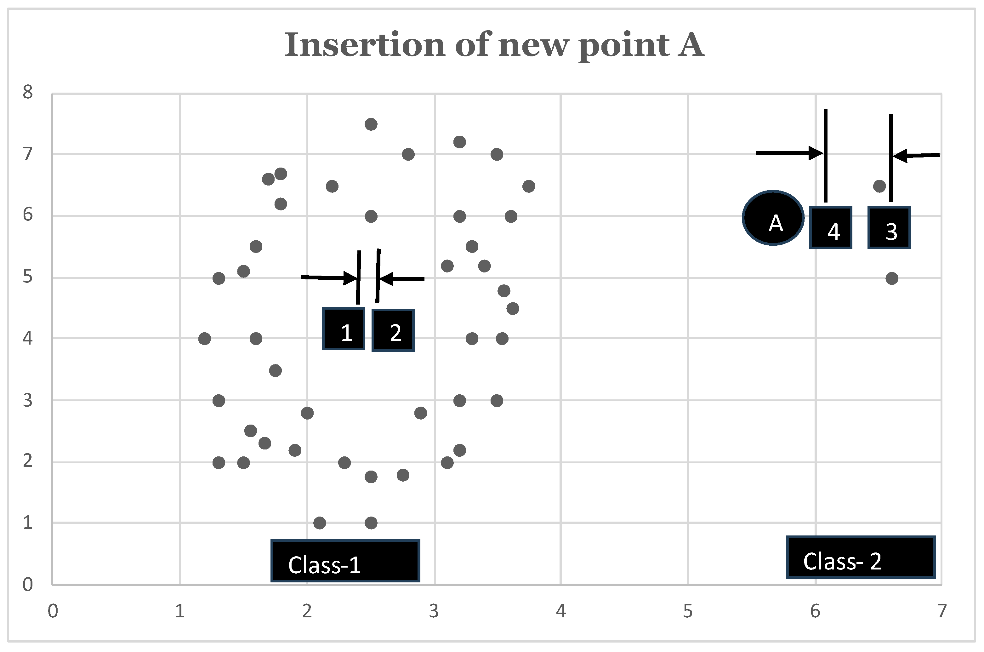
Figure 2.
Performance of MDEM algorithms as percentage of the best algorithms under k-fold cross validation
Figure 2.
Performance of MDEM algorithms as percentage of the best algorithms under k-fold cross validation
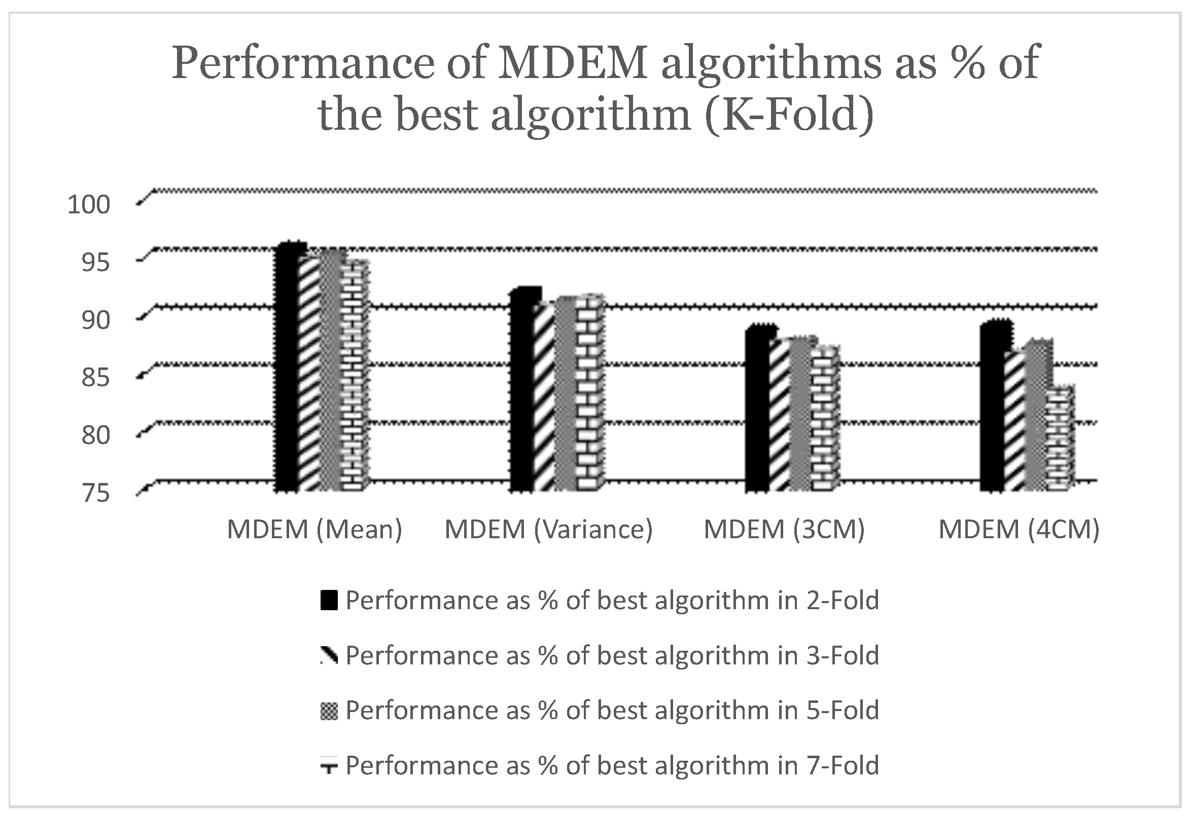
Figure 3.
Performance of MDEM algorithms as percentage of the best algorithm under stratified k-fold cross validation
Figure 3.
Performance of MDEM algorithms as percentage of the best algorithm under stratified k-fold cross validation
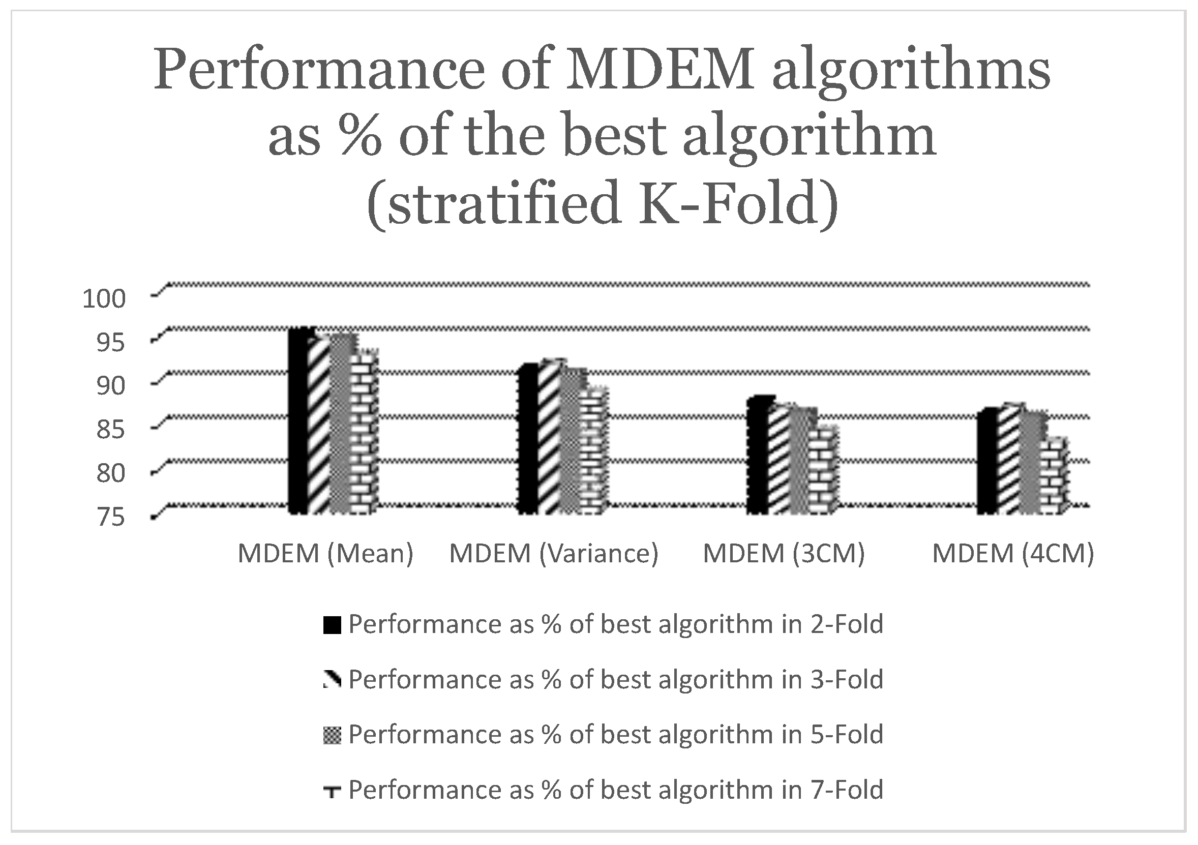

Table 1.
Descriptive statistics
| No | Attribute description | Attribute type | Average value |
| 1 | Number of times pregnant | Numeric | 3.85 |
| 2 | Plasma glucose concentration in 2h in an oral glucose tolerance test | Numeric | 120.89 |
| 3 | Diastolic blood pressure (mm HG) | Numeric | 69.11 |
| 4 | Triceps skin fold thickness (mm) | Numeric | 20.54 |
| 5 | Serum insulin level () | Numeric | 79.80 |
| 6 | Body Mass Index (BMI) () | Numeric | 31.99 |
| 7 | Diabetes Pedigree Function | Numeric | 0.47 |
| 8 | Age (years) | Numeric | 33.24 |
| 9 | Output variable | Nominal; 1: Diabetic; 0: Non-Diabetic | 268 Diabetic; 500 non-diabetic |
Table 2.
Performance analyses of different algorithms using k-fold cross validation technique
| Algorithm | 2-Fold | 3-Fold | 5-Fold | 7-Fold |
| MDEM (Mean) | 73.43% | 73.57% | 73.44% | 73.16% |
| MDEM (Variance) | 70.51% | 70.37% | 70.37% | 70.93% |
| MDEM (3rd Central Moment) | 68.00% | 68.00% | 67.74% | 67.46% |
| MDEM (4th Central Moment) | 68.29% | 67.17% | 65.23% | 64.81% |
| Logistic Regression (LR) | 74.83% | 77.47% | 76.92% | 77.34% |
| Random Foresh (RF) | 75.94% | 76.22% | 76.92% | 76.49% |
| Support Vector Machine (SVM) | 76.63% | 77.19% | 77.06% | 77.48% |
| K Nearest Neighbor (KNN) (n = 3) | 69.82% | 72.05% | 71.49% | 71.78% |
| K Nearest Neighbor (KNN) (n = 5) | 70.38% | 71.91% | 73.30% | 74.28% |
| K Nearest Neighbor (KNN) (n = 7) | 72.32% | 72.74% | 72.05% | 73.02% |
| Neural Network (Hidden Layer = 1, Epoch = 50) | 67.04% | 66.34% | 67.05% | 68.57% |
| Neural Network (Hidden Layer = 1, Epoch = 100) | 66.48% | 70.93% | 69.68% | 73.16% |
| Neural Network (Hidden Layer = 1, Epoch = 150) | 70.65% | 72.19% | 72.32% | 75.82% |
| Neural Network (Hidden Layer = 2, Epoch = 50) | 67.18% | 67.88% | 68.02% | 70.52% |
| Neural Network (Hidden Layer = 2, Epoch = 100) | 71.62% | 75.39% | 74.41% | 74.55% |
| Neural Network (Hidden Layer = 2, Epoch = 150) | 73.15% | 76.22% | 75.81% | 76.64% |
| Neural Network (Hidden Layer = 3, Epoch = 50) | 67.73% | 72.33% | 71.22% | 73.58% |
| Neural Network (Hidden Layer = 3, Epoch = 100) | 73.01% | 75.11% | 76.23% | 76.22% |
Table 3.
Performance analyses of different algorithms using stratified k-fold cross validation technique
Table 3.
Performance analyses of different algorithms using stratified k-fold cross validation technique
| Algorithm | 2-Fold | 3-Fold | 5-Fold | 7-Fold |
| MDEM (Mean) | 73.99% | 73.02% | 73.85% | 73.85% |
| MDEM (Variance) | 70.79% | 70.93% | 70.78% | 70.65% |
| MDEM (3rd Central Moment) | 68.01% | 67.03% | 67.31% | 67.18% |
| MDEM (4th Central Moment) | 66.90% | 67.18% | 67.03% | 66.07% |
| Logistic Regression (LR) | 77.33% | 77.05% | 77.75% | 77.47% |
| Random Foresh (RF) | 75.66% | 76.78% | 77.33% | 79.42% |
| Support Vector Machine (SVM) | 76.50% | 76.36% | 77.61% | 77.48% |
| K Nearest Neighbor (KNN) (n = 3) | 72.60% | 73.99% | 73.30% | 73.99% |
| K Nearest Neighbor (KNN) (n = 5) | 73.58% | 73.72% | 74.27% | 74.28% |
| K Nearest Neighbor (KNN) (n = 7) | 74.55% | 73.58% | 73.57% | 73.30% |
| Neural Network (Hidden Layer = 1, Epoch = 50) | 66.62% | 66.76% | 67.32% | 69.40% |
| Neural Network (Hidden Layer = 1, Epoch = 100) | 68.70% | 73.16% | 70.65% | 71.36% |
| Neural Network (Hidden Layer = 1, Epoch = 150) | 70.10% | 73.58% | 74.13% | 74.83% |
| Neural Network (Hidden Layer = 2, Epoch = 50) | 71.63% | 71.22% | 68.15% | 69.68% |
| Neural Network (Hidden Layer = 2, Epoch = 100) | 67.87% | 74.97% | 74.13% | 73.45% |
| Neural Network (Hidden Layer = 2, Epoch = 150) | 72.32% | 75.66% | 75.52% | 76.51% |
| Neural Network (Hidden Layer = 3, Epoch = 50) | 69.40% | 68.15% | 71.20% | 73.43% |
| Neural Network (Hidden Layer = 3, Epoch = 100) | 74.13% | 73.72% | 74.55% | 75.24% |
Disclaimer/Publisher’s Note: The statements, opinions and data contained in all publications are solely those of the individual author(s) and contributor(s) and not of MDPI and/or the editor(s). MDPI and/or the editor(s) disclaim responsibility for any injury to people or property resulting from any ideas, methods, instructions or products referred to in the content. |
© 2025 by the authors. Licensee MDPI, Basel, Switzerland. This article is an open access article distributed under the terms and conditions of the Creative Commons Attribution (CC BY) license (http://creativecommons.org/licenses/by/4.0/).
Copyright: This open access article is published under a Creative Commons CC BY 4.0 license, which permit the free download, distribution, and reuse, provided that the author and preprint are cited in any reuse.


