
Submitted:
08 January 2025
Posted:
08 January 2025
You are already at the latest version
Abstract
In this study, we propose a solution for automatically measuring body circumferences by utilizing the built-in LiDAR sensor in mobile devices. While traditional body measurement methods primarily rely on 2D images or manual measurements, this research leverages 3D depth information to enable more accurate and efficient measurements. By employing HRNet-based keypoint detection and transfer learning through deep learning, the precise locations of body parts are identified and combined with depth maps to automatically calculate body circumferences. Experimental results demonstrate that the proposed method exhibits a relative error of up to 8\% for major body parts such as waist, chest, hip, and buttock circumferences, with waist and buttock measurements recording low error rates below 4\%. Although some models showed error rates of 7.8\% and 7.4\% in hip circumference measurements, this was attributed to the complexity of 3D structures and the challenges in selecting keypoint locations. Additionally, the use of depth map-based keypoint correction and regression analysis significantly improved accuracy compared to conventional 2D-based measurement methods. The real-time processing speed was also excellent, ensuring stable performance across various body types.
Keywords:
LiDAR
; HRNet
; Deep Learning
; Keypoint
1. Introduction
The fourth industrial revolution is bringing about rapid changes across various industries through the convergence of innovative technologies such as Artificial Intelligence (AI), Big Data, the Internet of Things (IoT), and robotics. These technological advancements assist human tasks, create new business models, and contribute to maximizing overall societal efficiency. In particular, the field of computer vision, integrated with deep learning-based AI technologies, is opening up diverse application possibilities by enabling computers to understand and interpret visual information through images or videos. Computer vision is a technology that allows computers to analyze and recognize visual data similarly to humans by utilizing advanced techniques such as machine learning, deep learning, and image processing. This field is divided into various subfields, including object recognition, facial recognition, image segmentation [8], and motion recognition, and is employed as a core technology in numerous industries such as autonomous driving, security systems, medical image analysis [6], and sports analytics [10,15,17]. For example, object recognition technology [11] is essential for autonomous vehicles to accurately recognize vehicles, pedestrians, and traffic lights on the road, while facial recognition technology is used in security systems for identity verification and access control. Additionally, image segmentation technology [21] is utilized to accurately identify and analyze tumors or other lesions in medical imaging, and motion recognition technology is applied in analyzing the movements of athletes or in human behavior recognition systems. However, these computer vision technologies are primarily based on 2D images or video data as shown in the Figure 1, and accurate length measurement solutions in 3D space have not yet been sufficiently developed. 3D length measurement can play a significant role in various fields such as architecture, manufacturing, healthcare, and fashion, and can greatly enhance accuracy and efficiency in personalized services like body size measurement.
In recent years, LiDAR (Light Detection And Ranging) [3] technology has rapidly advanced by expanding its range of applications. LiDAR is a technology that calculates distances by emitting lasers and measuring the time it takes for the reflected light from objects to return, thereby generating high-resolution 3D point clouds. This technology is utilized in various fields such as autonomous vehicles, drones, robotics, and Geographic Information Systems (GIS), and it particularly excels in precise data collection and analysis in 3D spaces. Additionally, LiDAR sensors embedded in mobile devices provide high-resolution depth information in consumer-grade devices, enabling general users to easily utilize 3D data. LiDAR sensors can operate in both vertical and horizontal directions and can create precise 3D models of objects through multi-directional scanning. Thanks to these characteristics, LiDAR is widely used in specialized fields such as surveying, geomorphology, archaeology, laser guidance, and high-resolution map-making. In particular, high-resolution 3D scanning has established itself as an essential tool for precisely analyzing complex terrains and structures. However, up to now, LiDAR technology has been primarily used in specialized equipment or industrial settings, and its utilization in everyday life has been limited. This is due to the high cost of equipment and complex maintenance requirements, making it perceived as a technology that is difficult for general users to access. Therefore, developing a more affordable and user-friendly 3D measurement solution by leveraging LiDAR sensors embedded in mobile devices has become an important research task. One of the application areas for this technology, body size measurement, plays a crucial role in various fields such as the apparel industry, healthcare, and fitness. Traditionally, body measurements have been carried out in a manual manner, which can be time-consuming and inconvenient for users. Especially when purchasing clothing online, accurately measuring body sizes is essential, but until now, there has been the inconvenience of users having to measure their dimensions using measuring tools themselves. To address these issues, the development of automatic body size measurement technology is necessary.
The goal is to develop 3D length measurement technology by utilizing the standard 2D RGB camera and built-in LiDAR sensor of mobile devices to extract depth information alongside 2D images of subjects. Through this, we seek to provide a platform that allows easy measurement of body dimensions in everyday life without the need for specialized 3D equipment. Software utilizing mobile devices can be implemented at a low cost and can significantly enhance user convenience by measuring lengths in real time and providing immediate results. Additionally, an intuitive user interface increases accessibility to the technology and efficiently uses energy and resources, thereby reducing time and energy consumption. Specifically, body size is an important metric in clothing purchases. Previously, users had to measure their dimensions themselves, but the automatic dimension measurement platform proposed in this study supports users in easily measuring their body dimensions, thereby greatly enhancing the convenience of online shopping. This is expected to improve user experience and have positive effects such as reducing return rates.
This study contributes to several important aspects. First, it developed a technology for accurately measuring 3D lengths by utilizing the LiDAR sensor embedded in mobile devices without relying on specialized 3D equipment. Second, it introduced a keypoint detection technique based on the HRNet model and improved measurement accuracy by accurately identifying the positions of body parts through transfer learning. Third, it developed an algorithm that effectively integrates 2D RGB images and 3D depth maps, enabling accurate length measurements in three-dimensional space. Lastly, it implemented an algorithm that automatically measures the circumferences of body parts based on images captured from the front and side, and demonstrated high accuracy through experiments. This paper is structured as follows. Section 2 reviews related studies and discusses the distinctions from the current research. Section 3 provides a detailed explanation of the principles behind storing 3D depth information using a mobile phone LiDAR Sensor. Section 4 introduces the proposed methodology, detailing the processes of data collection, preprocessing, keypoint detection and merging, and the body circumference measurement algorithm. Section 5 presents the experimental setup and results, validating the effectiveness of the proposed method through result analysis. Finally, Section 6 discusses the limitations of this study and outlines directions for future research.
2. Mobile Device 3D Measurement Technology
As shown in Figure 1, research on body measurement has primarily been based on 2D image analysis. These studies have focused on methods that detect the positions of body parts using pose estimation techniques and calculate circumferences based on them. In particular, high-resolution pose estimation models like HRNet are effective in accurate keypoint detection, but due to the limitations of 2D images, 3D depth information is not reflected, restricting the accuracy of measurements [16]. Research on 2D image-based body measurement has primarily relied on pose estimation and keypoint detection. The HRNet model excels at accurately detecting keypoints of body parts while maintaining high-resolution representations, allowing precise identification of the locations of various body parts [16]. However, these methods have limitations in that they do not consider depth information, thereby failing to accurately reflect the 3D structure of the body. For example, they may not account for depth variations of the body or distortions due to various postures, which can reduce measurement accuracy [5]. Additionally, [2] proposed a method to track body movements through real-time pose estimation, but it is primarily focused on motion analysis and is not suitable for static body circumference measurements [12]. Attempted 3D pose estimation, but still did not fully incorporate depth information from 2D images, resulting in limitations in accuracy.
2.1. 3D Measurement Technologies and Applications of LiDAR
3D measurement technologies overcome the limitations of 2D images and enable more accurate body measurements. Representative 3D measurement technologies include Structured Light [4], Stereo Vision [1], and LiDAR [3]. Among these, LiDAR is a technology that can generate high-resolution 3D point clouds by measuring distances to objects using lasers, and is widely utilized in various fields such as autonomous vehicles, robotics, and Geographic Information Systems (GIS). LiDAR technology has several advantages. It allows for highly accurate distance measurements through laser emission and reflection, can generate a large number of point clouds at high speeds enabling real-time data processing, and can be utilized in various fields such as construction, surveying, archaeology, and environmental monitoring [13]. However, in the field of body measurement, the application of LiDAR is relatively insufficient. This is mainly due to the need for specialized equipment, high costs, and complex data processing requirements, making it perceived as a technology that is difficult for general users to access [14,19]. Although some recent studies have proposed body recognition and measurement methods using LiDAR data, these studies remain mostly at the research stage, and implementation as practical solutions is limited [7].
2.2. LiDAR-Based Body Measurement Technology
Recently, research on body measurement utilizing LiDAR sensors has been increasing. For example, [7] proposed a method to automatically recognize and measure human body parts using LiDAR data. In this study, 3D point clouds from LiDAR were used to accurately identify various body parts and measure body circumferences based on them. However, this method primarily assumes measurements in a fixed environment, limiting its applicability in various everyday situations. Another study [20] proposed a method to predict the locations of body parts based on LiDAR data using a deep learning model. This study effectively utilized depth information from LiDAR to create a 3D body model, showing higher accuracy than conventional 2D image-based methods, but research on real-time processing and user-friendly interface implementation is still lacking.
2.3. Data Collection for 3D Measurement
In this study, uniform 3D data, such as cylindrical object and mannequin, were used to create initial datasets and later expanded to actual human body measurements. The experiments began with relatively simple models that resemble specific human body parts to minimize deformation, enhance the accuracy of the measurement algorithm, and enable a systematic evaluation across various body parts. Notably, previous studies such as [7] and [20] primarily conducted experiments on real human subjects. In contrast, this study verified the performance of the algorithm in the early stages using uniform 3D objects. This approach helped secure fundamental accuracy and minimize variables that could arise when measuring different body parts. Additionally, the use of cylindrical object and mannequin ensured data consistency, which played a critical role in the training and evaluation processes of the deep learning model.
2.4. Limitations of Existing Studies and Differentiation of This Study
Existing LiDAR-based body measurement studies have primarily aimed at applications in specialized environments, limiting the development of practical mobile application solutions. Additionally, these studies have mostly focused on body recognition and basic measurements, with many shortcomings remaining in precise measurements such as body circumferences. In particular, research utilizing LiDAR sensors embedded in mobile devices is very limited, resulting in a lack of specific implementation methods and evaluations necessary for developing body measurement solutions for everyday life.
This study proposes a solution for automatically measuring body circumferences by utilizing LiDAR sensors embedded in mobile devices to overcome these limitations. While existing studies primarily assume specialized equipment and environments, this research focuses on developing a body measurement platform that can be easily accessed in everyday life by leveraging low-cost mobile devices. Additionally, by combining HRNet-based keypoint detection with transfer learning through deep learning, the precise locations of body parts were identified and integrated with 3D depth information, enabling more accurate body circumference measurements. This approach was experimentally demonstrated to achieve both higher accuracy and practicality compared to conventional 2D image-based methods. This study overcame the limitations of existing 2D image-based body measurement research and 3D measurement technologies using LiDAR by developing a practical body measurement solution utilizing mobile devices, using uniform 3D data such as cylinder and mannequin. Through this, the accuracy of the body circumference measurement algorithm was enhanced, and a foundation was established for systematically evaluating measurements of various body parts. Furthermore, by integrating HRNet-based keypoint detection with transfer learning through deep learning and combining it with 3D depth information, higher accuracy, and practicality were achieved compared to existing methods.
3. Proposed Method
3.1. Merging Keypoints and 3D Data
Body circumference measurement in this study is divided into three main stages. The first stage involves detecting the endpoints of the body parts to be measured from photographs taken from the front and side. The second stage is calculating the circumference between the detected endpoints, and the third stage is estimating the total circumference of the desired body part based on the measurements taken from the front and side. In this section, we describe the detailed methodology and implementation process for each stage and discuss the technical improvements introduced to overcome existing limitations.
First, in the initial stage of body circumference measurement, accurately detecting the endpoints of body parts is essential. To achieve this, we utilized the Human Pose Estimation using the High-Resolution Representations (HRNet) model [16]. HRNet excels at maintaining high-resolution representations while precisely detecting keypoints of the body, allowing for accurate identification of various body parts’ locations. However, the basic HRNet model provides only a limited number of keypoints necessary for standard pose estimation, which restricts its ability to sufficiently cover all the endpoints required for body circumference measurement.
To overcome these limitations, we applied Transfer Learning in this study. Specifically, we labeled 1,000 images of people by categorizing them into two groups: upper body and lower body. In the upper body category, we labeled the endpoints of the chest and waist, and in the lower body category, we labeled the hip and buttock as keypoints. By further training the HRNet model using this labeled dataset, we aimed to expand the model’s limited keypoint detection capabilities. The transfer learning process involved collecting 1,000 images of people divided into upper and lower body categories, manually labeling the keypoints for the chest, waist, buttock, hips, and femoral condyles in each image, and setting up based on the pre-trained HRNet model. We then retrained the last few layers of the HRNet model using the labeled dataset to accurately detect the new keypoints, evaluated the model’s performance with a validation dataset, and adjusted hyperparameters as necessary.
In the second stage, we calculate the circumference between the detected endpoints from the front and side views. This calculation is primarily based on the Euclidean distance. Specifically, we define two keypoints as and , and represent the distance between the two points as . The Euclidean distance formula is as follows Equation (1):
Under the assumption that the y-axis positions of the two points are identical, the straight-line distances in the x-axis direction are summed to approximate the circumference between the two points. Represents this calculation follows Equation (2):
However, as mentioned earlier, the keypoints detected in 2D images do not correspond to their actual positions in 3D space, so simply doubling the circumference of the front part introduces errors. This is because the boundary surfaces of the object from the camera’s viewpoint do not coincide with the actual boundary surfaces. Considering the angle between the camera’s line of sight and the object’s boundary surface, the distance from the camera to the center of the object, the distance from the center of the object to the boundary surface, and the actual length of the object’s boundary surface, the error can be calculated as follow Equation (3):
Therefore, the error resulting from the difference between the 2D keypoints and the 3D keypoints is represented by a length of . For this reason, simply multiplying the circumference of the front part by two to estimate the total circumference leads to inaccurate results. Additionally, to correct the positions of the keypoints detected in 2D images to their accurate locations in 3D space, this study introduced a correction process utilizing a depth map. First, a depth map of the same scene as the RGB image captured using the iPhone’s LiDAR sensor is generated. A depth map indicates that lower values are closer to the object and higher values are further away from the object. Next, the Canny edge algorithm is applied to the depth map to detect points where the depth value changes abruptly [18]. This is useful for accurately identifying the object’s boundary surfaces. Then, the coordinates of the keypoints detected in the 2D RGB image are transformed to match the scale of the depth map and moved to the nearest edge point. This process includes the following two steps: matching the resolution of the RGB image with that of the depth map.
First, a depth map of the same scene as the RGB image captured using the iPhone’s LiDAR sensor is generated. A depth map indicates that lower values are closer to the object and higher values are further away from the object. Next, the Canny edge algorithm is applied to the depth map to detect points where the depth value changes abruptly. This is useful for accurately identifying the object’s boundary surfaces. Then, the coordinates of the keypoints detected in the 2D RGB image are transformed to match the scale of the depth map and moved to the nearest edge point. This process includes the following two steps: matching the resolution of the RGB image with that of the depth map.
For example, if the RGB image size is () and the depth map size is (), the keypoint coordinates of the RGB image are divided by 7.5 to convert them to the depth map coordinates. Then, the nearest edge point is searched from the transformed keypoint coordinates, and the keypoint is moved to that point. Finally, to verify that the corrected keypoints coincide with the actual boundary surfaces of the object, the positions on the depth map and the visual positions on the RGB image are compared and analyzed. Through this correction process, the keypoints detected in the 2D image were adjusted to match their actual positions in 3D space. This significantly improved the accuracy of body circumference measurements. In the keypoints correction stage, the circumferences measured from the front and side are integrated to estimate the total circumference of the body part. To do this, a regression equation was derived by multiplying the circumference values measured from the front and side by a certain constant to calculate the total circumference. This equation was applied only when measuring the dimensions of actual people, and experiments were conducted to find the optimal constant for each body part. The results are as follows Equation (4):
These constants were derived through regression analysis by comparing the actual circumferences of various body parts with the measured values. This allowed for the accurate estimation of the total circumference based on the measurements taken from the front and side. Additionally, regression analysis is a statistical method that derives constants based on measured data and actual data. In this study, measurement data for various body parts were collected, and constant values were derived based on this data. This enabled the identification of optimal constant values that minimize measurement errors.
3.2. Utilization of Uniform 3D Data
In this study, to enhance the accuracy and consistency of the body measurement algorithm, experiments were conducted using uniform 3D data such as cylinder and mannequin. These standardized 3D objects, which closely resemble the human body while exhibiting minimal deformation, were useful for systematically verifying the performance of the algorithm in its initial stages. Cylinders, with their simple structure, are ideal objects for evaluating whether the algorithm can accurately measure complex body structures. Additionally, mannequin, which mimic the shape of the human body, were used to test the measurement accuracy of various body parts. Through this approach, it was confirmed that the algorithm could accurately measure body parts of different shapes and sizes. The experimental procedure involved first capturing RGB images and depth maps of the cylinder and mannequin from various angles using an iPhone’s LiDAR sensor. Using an HRNet-based keypoint detection model, the endpoints of the major parts of each object were detected. The detected keypoints were then adjusted to their accurate positions in 3D space through the aforementioned correction process. Based on the corrected keypoints, circumferences were calculated, and the total circumference was estimated by integrating the measurements taken from the front and side views. The measured circumference values were compared with the actual values to evaluate the accuracy of the algorithm. Through these experiments, the accuracy and consistency of the proposed body circumference measurement algorithmwere systematically validated, and methods to minimize errors in measuring various body parts were established.
The body circumference measurement algorithm proposed in this study consists of the following key components. First, RGB images and depth maps are extracted at the same scale to facilitate subsequent data merging and analysis. Second, the keypoints detected by the HRNet model are adjusted to accurate 3D positions through a depth map-based correction process. Third, the circumferences of body parts are calculated using the corrected keypoints, and the total circumference is estimated by integrating the measurements taken from the front and side views. Finally, a regression equation was derived to estimate the total circumference based on the measured circumferences from the front and side views, enabling accurate measurements. Additionally, to enhance the efficiency of the algorithm, the following optimization techniques were introduced. First, model lightweighting and parallel processing were employed to enable real-time body circumference measurements. Data captured from various angles and lighting conditions were utilized to improve the model’s generalization performance. Furthermore, filtering techniques were applied to minimize noise in the depth maps.
3.3. Experimental Environment and Dataset
As shown in Figure 2 and Figure 3, uniform 3D data such as cylinder and mannequin were used to ensure the consistency and reproducibility of the experiments. In Figure 2 and Figure 3, (b) in each figure is a depth map visualizing the distance between the camera and the object. Lower depth values are represented by darker colors, while higher depth values are represented by brighter colors, visually depicting the three-dimensional structure of the object. The actual circumference of the cylinder is 17.27cm, and the estimated circumference measured by LiDAR is 17.68cm, demonstrating an accuracy within a 3% error margin. The results for the cylinder and mannequin are shown in Table 11, respectively. The regression equation is tailored to humans, and the Mannequin has a different shape compared to an actual person, resulting in slightly larger errors. The experimental environment involved using a model equipped with an iPhone’s LiDAR sensor to simultaneously collect RGB images and depth maps, maintaining data consistency by photographing objects under the same lighting conditions and fixed distances. Through such standardized datasets, the performance of the algorithm could be systematically evaluated, and errors that could occur in measuring various body parts could be analyzed.
Figures (a) and (c) in Figure 4 visualize the distance measurements before correction for the cylinder and mannequin, respectively. Distance values exceeding 12cm between adjacent pixels were observed, which can be interpreted as the distance between the object and the background rather than within the object itself. Points where the values suddenly increase indicate locations beyond the object’s boundary. In contrast, Figures (b) and (d) show the distance measurements after correction for the cylinder and mannequin, respectively, with the maximum value not exceeding 1cm. This suggests that by detecting edges using depth values and correcting the keypoints, the lengths to the object’s boundary surfaces were accurately measured.
4. Actual Model Measurement
Figure 5 shows photos taken to capture images of the upper and lower body parts of a person, respectively. Due to the characteristics of the iPhone’s LiDAR sensor, the depth map size is , so it was extracted from the RGB image at the same scale. This maintains consistency between images, ensuring accuracy in subsequent data merging and correction processes.
Figure 5(c) shows the edge image obtained by applying the Canny Edge algorithm to the depth image. Canny Edge Detection is an algorithm used to find edges in images, effectively detecting points where depth values change sharply. This algorithm not only identifies points with sudden changes in depth values but also helps to accurately detect the actual boundary surfaces of objects. By first identifying areas with significant depth changes and then connecting points with high depth change intensity, the algorithm can more precisely detect the actual boundary surfaces of the object, rather than meaningless edges. Figure 6 shows arbitrary keypoints manually detected from the RGB image. The process involves manually selecting keypoints first and then automatically correcting them using deep learning. To make the correction effect more apparent, the manually selected keypoints were marked slightly offset from the boundary. The size of the RGB image is , and the size of the depth map is . Since the ratio between the RGB image and the depth map is 7.5, the keypoint coordinates detected in the RGB image were divided by 7.5 to convert them into depth map coordinates. The transformed keypoints were adjusted to match the resolution of the depth map, which plays an important role in maintaining the accurate alignment between the two datasets.
Figure 7 and Figure 8 illustrate the keypoint correction process before and after applying the edge algorithm. Figure 7 shows the coordinates of the keypoints manually identified, while Figure 8 presents the results corrected based on the edge algorithm. In Figure 7 and Figure 8, the y-axis represents the distance between the subject’s pixels and the background, and the x-axis represents the pixel index. In Figure 7, when a keypoint is located outside the subject, the distance between the subject and the wall behind exceeds 10cm. In contrast, when a keypoint is located inside the subject, it shows a short distance within a few centimeters. The keypoint correction was performed by moving the keypoints to the coordinates of the nearest edges to align them with their actual positions in 3D space. After correction, the keypoints coincide with the edges detected in the depth map, enabling a more accurate representation of the object’s actual boundary surfaces.
5. Results
To evaluate the performance of the 3D landmark measurement algorithm developed in this study, experiments were conducted on four body parts: waist circumference, chest circumference, buttock circumference, and hip circumference. For each body part, the total circumference was estimated based on front and side measurements of a total of four models, and the errors compared to actual measurements were analyzed. Table 3, Table 2, Table 4, and Table 5 shows the results comparing the estimated circumferences with the actual measurements for each body part.
Overall, the algorithm recorded relative errors within 8% for most body parts, and particularly showed low error rates below 4% for waist and hip circumferences. This indicates that the algorithm effectively applied keypoint correction and regression analysis methods to enhance the accuracy of body circumference measurements. In measuring the buttock circumference of actual human models, the error rates for Person 1 and Person 2 were relatively high at 7.8% and 7.4%, respectively. This can be attributed to the complex 3D structure of the buttock area and the difficulty in selecting keypoint positions. On the other hand, in measuring hip circumference, all subjects recorded low error rates within 2.6%, confirming the stability of the algorithm.
Additionally, as shown in Figure 7 and Figure 8, keypoint correction utilizing the depth map overcame the limitations of 2D image-based measurements and enabled more precise 3D measurements. Experimental results confirmed that the correction process through the depth map contributed to the accuracy improvement for each body part. Moreover, the real-time processing speed in actual experimental environments was sufficiently fast, suggesting practical application possibilities. The overall performance of the algorithm proposed in this study holds significant meaning for the transition from professional equipment to lightweight mobile devices. The conventional 2D length measurement methods were limited in measurement accuracy due to the inability to reflect depth information of the body, but this algorithm overcomes such limitations by effectively utilizing 3D information.
6. Conclusions
Measurement errors primarily occur when the HRNet model fails to accurately detect keypoints, when the resolution and precision of the depth map are low, when the constants derived through regression analysis do not exactly match the actual circumference of body parts, when shooting conditions are inconsistent, and when there is poor alignment between the depth map and the RGB image.
In Section 5, the process of merging keypoints and 3D data for body circumference measurements is described in detail. Accurate locations of body parts were determined through keypoint detection based on the HRNet model and transfer learning, and the limitations of 2D images were overcome through keypoints correction using the depth map. Additionally, the accuracy and consistency of the algorithm were systematically evaluated using uniform 3D data such as cylinder and mannequin. Through this approach, this study was able to achieve higher accuracy and practicality compared to existing 2D image-based body measurement methods, suggesting potential applications in various fields.
In this study, a 3D measurement algorithm was developed to enable precise measurements of key body parts such as waist circumference, chest circumference, hip circumference, and others. Experimental results demonstrated the high accuracy of the algorithm by recording low relative errors within 8% for most body parts. In particular, the keypoint correction technique using the depth map contributed to overcoming the limitations of 2D-based measurement methods and realizing more precise 3D measurements. This study provides a foundation that can be effectively utilized for real-time body measurement and analysis in various fields, including fitness, healthcare, and the clothing industry. Furthermore, the excellent real-time processing speed of the algorithm confirmed in the experiments serves as a significant advantage for practical applications. However, this study was conducted on a limited number of models and has several limitations, such as somewhat higher error rates for certain body parts. To overcome these limitations, future research needs to involve large-scale experiments with more diverse subjects and the development of additional correction techniques. In summary, the 3D landmark measurement algorithm proposed in this study offers higher accuracy and practicality compared to existing 2D methods, suggesting potential applications in various fields. Through continuous improvement and expansion of the algorithm, the establishment of a more precise and reliable body measurement system is anticipated.
Acknowledgments
paper was supported by Konkuk University Researcher in 2024.
References
- Borangiu, T.; Dumitrache, A. Robot arms with 3D vision capabilities. INTECH Open Access Publisher, 2010.
- Cao, Z.; Simon, T.; Wei, S.-E.; Sheikh, Y. Realtime multi-person 2d pose estimation using part affinity fields. In Proceedings of the IEEE conference on computer vision and pattern recognition; pp. 7291–7299.
- Collis, R. T. H. Lidar. Applied optics; 9 (8), pp. 1782–1788, 1970.
- Forbes, A.; De Oliveira, M.; Dennis, M. R. Structured light. In Nature Photonics; 15 (4), pp. 253–262, 2021.
- He, K.; Zhang, X.; Ren, S.; Sun, J. Deep residual learning for image recognition. In Proceedings of the IEEE conference on computer vision and pattern recognition; pp. 770–778, 2016.
- Heo, S.-M.; Jung, S. J.; Kwak, H. M.; Jeong, Y. H.; Yang, S. M.; Lee, Y. H.; Kim, S. H. Dental Image Data Generation for Instance Segmentation using Generative Adversarial Networks. Quantitative Bio-Science; 42 (2), pp. 111–121, 2023.
- Huang, L.; Guo, H.; Rao, Q.; Hou, Z.; Li, S.; Qiu, S.; Fan, X.; Wang, H. Body dimension measurements of qinchuan cattle with transfer learning from liDAR sensing. Sensors; 19 (22), pp. 5046, 2019. [CrossRef]
- Jeong, H.; Moon, H.; Jeong, Y.; Kwon, H.; Kim, C.; Lee, Y.; Yang, S. M.; Kim, S. Automated Technology for Strawberry Size Measurement and Weight Prediction Using AI. IEEE Access, 2024. 10.1109/access.2024.3356118.
- Jia, Z.; Zaharia, M.; Aiken, A. Beyond data and model parallelism for deep neural networks. Proceedings of Machine Learning and Systems; 1, pp. 1–13, 2019.
- Kim, S.; Heo, S.-M.; Yang, S. M.; Kim, Y.; Han, J. S.; Jung, S. H. Instance segmentation guided by weight map with application to tooth boundary detection. Quantitative Bio-Science; 39 (2), pp. 159–167, 2020.
- Logothetis, N. K.; Sheinberg, D. L. Visual object recognition. Annual review of neuroscience; 19, pp. 577–621, 1996.
- Papandreou, G.; Zhu, T.; Kanazawa, N.; Toshev, A.; Tompson, J.; Bregler, C.; Murphy, K. Towards accurate multi-person pose estimation in the wild. In Proceedings of the IEEE conference on computer vision and pattern recognition; pp. 4903–4911, 2017.
- Raj, T.; Hashim, F. H.; Huddin, A. B.; Ibrahim, M. F.; Hussain, A. A survey on LiDAR scanning mechanisms. Electronics; 9 (5), pp. 741, 2020. [CrossRef]
- Royo, S.; Ballesta-Garcia, M. An overview of lidar imaging systems for autonomous vehicles. Applied sciences; 9 (19), pp. 4093, 2019. [CrossRef]
- Shapiro, L. Computer vision and image processing. Academic Press, 1992.
- Sun, K.; Xiao, B.; Liu, D.; Wang, J. Deep high-resolution representation learning for human pose estimation. In Proceedings of the IEEE/CVF conference on computer vision and pattern recognition; pp. 5693–5703, 2019.
- Szeliski, R. Computer vision: algorithms and applications. Springer Nature, 2022.
- Xu, Z.; Xu, B.; Wu, G. Canny edge detection based on Open CV. In 2017 13th IEEE international conference on electronic measurement & instruments (ICEMI); pp. 53–56, 2017.
- Yahya, M. A.; Abdul-Rahman, S.; Mutalib, S. Object detection for autonomous vehicle with LiDAR using deep learning. In 2020 IEEE 10th International conference on system engineering and technology (ICSET); pp. 207–212, 2020.
- Zhao, Z.; Zhuang, C.; Li, J.; Sun, H. LiDAR-based human pose estimation with MotionBERT. In 2024 IEEE International Conference on Mechatronics and Automation (ICMA); pp. 1849–1854, 2024.
- Minaee, S.; Boykov, Y.; Porikli, F.; Plaza, A.; Kehtarnavaz, N.; Terzopoulos, D. Image Segmentation Using Deep Learning: A Survey. In IEEE Transactions on Pattern Analysis and Machine Intelligence, 2022, 44(7), pp. 3523–3542. doi:10.1109/TPAMI.2021.3059968.
Figure 1.
An Example of Human Pose Estimation Using 2D Images.

Figure 2.
It shows the mannequin’s RGB photo (a), depth map (b), edge detection using the Canny algorithm (c), and keypoint detection in the depth map photo (d).
Figure 2.
It shows the mannequin’s RGB photo (a), depth map (b), edge detection using the Canny algorithm (c), and keypoint detection in the depth map photo (d).

Figure 3.
It shows Cylinder’s RGB photo (a), depth map (b), edge detection using the Canny algorithm (c), and keypoint detection in the depth map photo (d).
Figure 3.
It shows Cylinder’s RGB photo (a), depth map (b), edge detection using the Canny algorithm (c), and keypoint detection in the depth map photo (d).
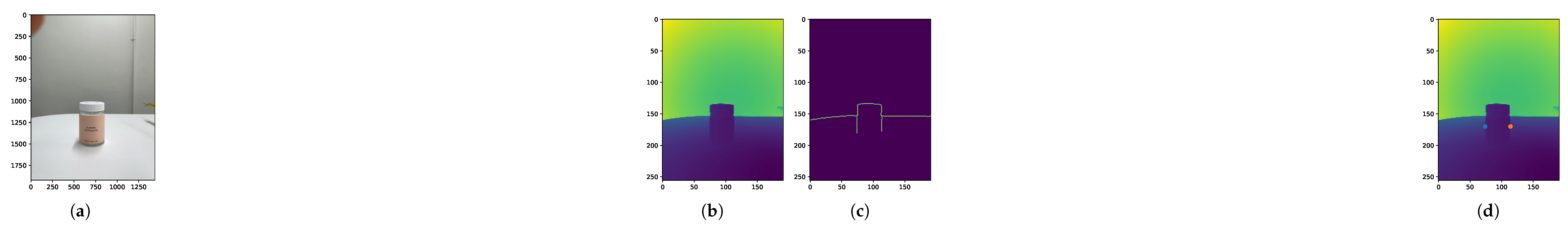
Figure 4.
These graphs display the cylinder’s uncorrected keypoints (a) and corrected keypoints (b), as well as the mannequin chest’s uncorrected keypoints (c) and corrected keypoints (d). In the corrected graphs, the y-axis automatically adjusts its maximum value as the pixel distance decreases.
Figure 4.
These graphs display the cylinder’s uncorrected keypoints (a) and corrected keypoints (b), as well as the mannequin chest’s uncorrected keypoints (c) and corrected keypoints (d). In the corrected graphs, the y-axis automatically adjusts its maximum value as the pixel distance decreases.
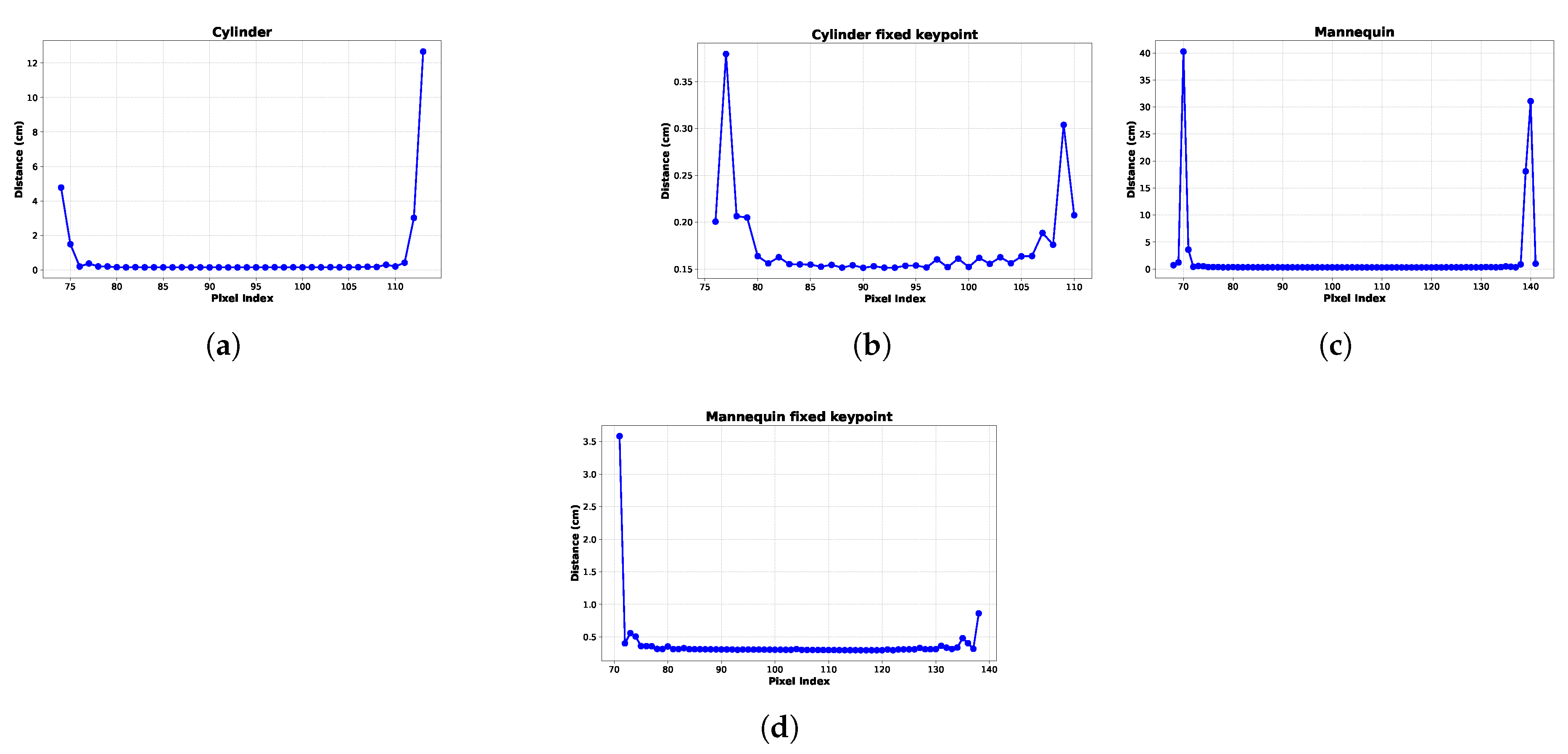
Figure 5.
The figure shows the model’s RGB capture (a), depth map conversion (b), and Canny edge detection (c).
Figure 5.
The figure shows the model’s RGB capture (a), depth map conversion (b), and Canny edge detection (c).
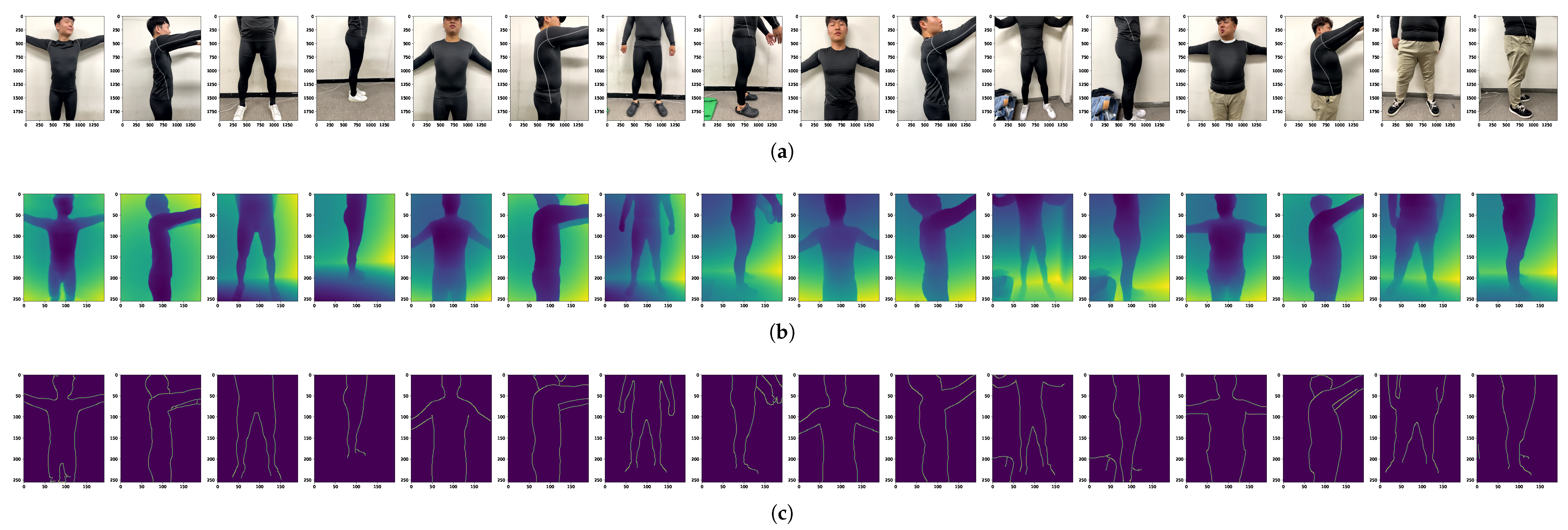
Figure 6.
Keypoints were placed at both endpoints of the waist, Chest, hips, and buttocks in the front and side views to measure the length of each body part. Person 1 is depicted in (a), Person 2 in (b), Person 3 in (c), and Person 4 in (d).
Figure 6.
Keypoints were placed at both endpoints of the waist, Chest, hips, and buttocks in the front and side views to measure the length of each body part. Person 1 is depicted in (a), Person 2 in (b), Person 3 in (c), and Person 4 in (d).

Figure 7.
Graphs showing the data before keypoint correction, with the y-axis representing the distance between the subject’s pixels and the background. Person 1 is depicted in (a), Person 2 in (b), Person 3 in (c), and Person 4 in (d).
Figure 7.
Graphs showing the data before keypoint correction, with the y-axis representing the distance between the subject’s pixels and the background. Person 1 is depicted in (a), Person 2 in (b), Person 3 in (c), and Person 4 in (d).
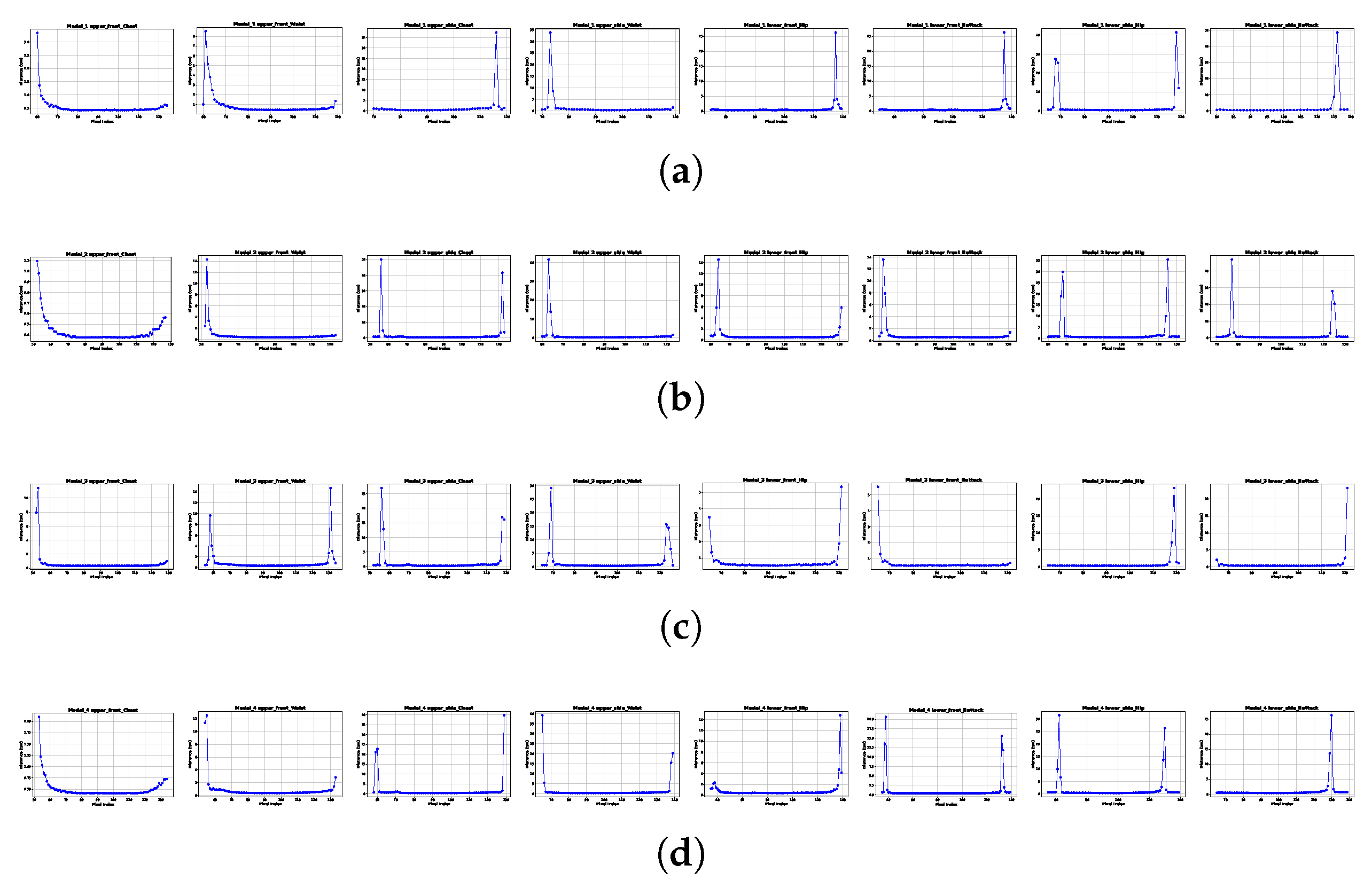
Figure 8.
Graphs showing the data after keypoint correction. The y-axis automatically adjusts its maximum value as the distance between pixels decreases. Person 1 is depicted in (a), Person 2 in (b), Person 3 in (c), and Person 4 in (d).
Figure 8.
Graphs showing the data after keypoint correction. The y-axis automatically adjusts its maximum value as the distance between pixels decreases. Person 1 is depicted in (a), Person 2 in (b), Person 3 in (c), and Person 4 in (d).
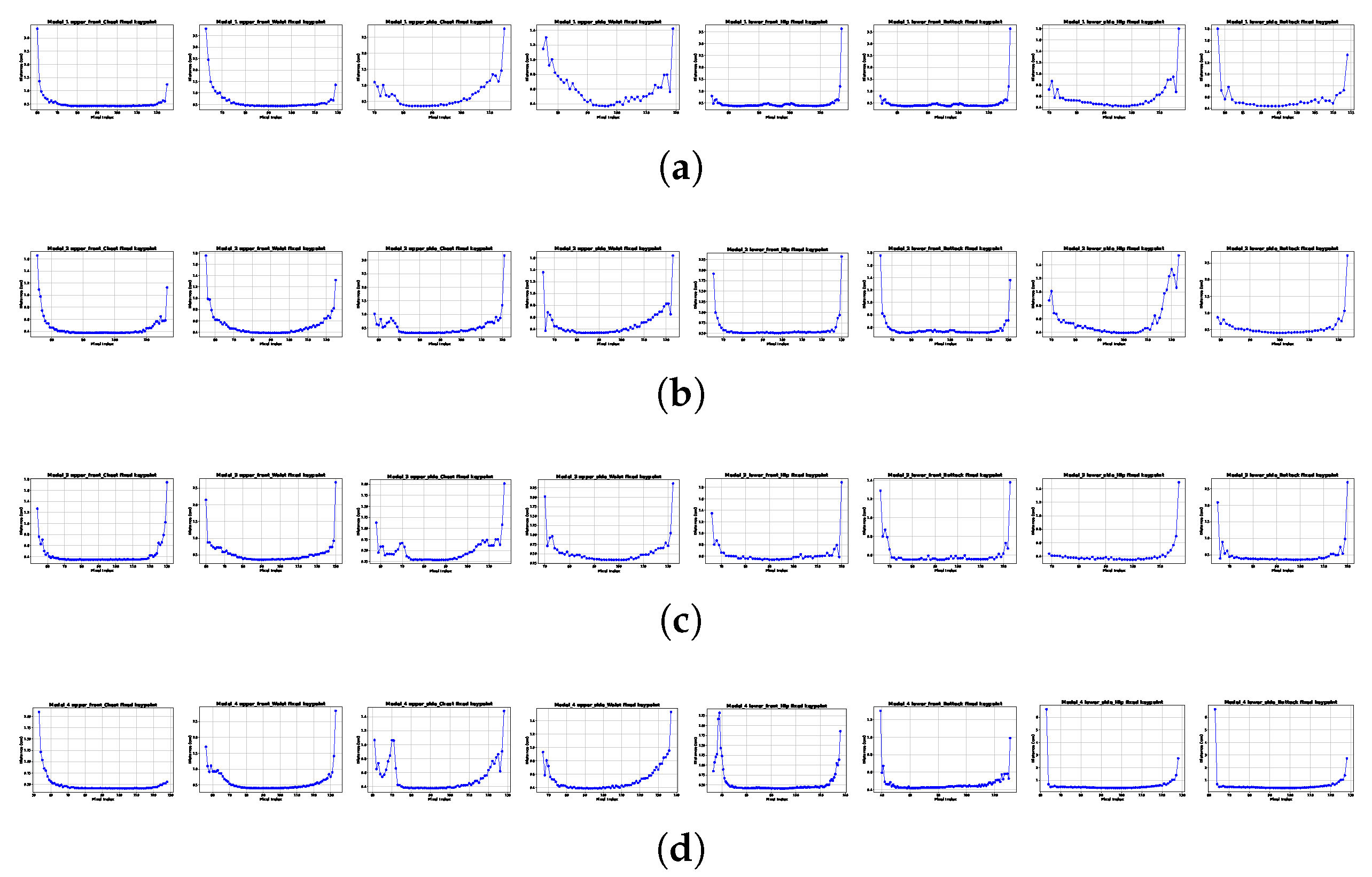

Table 1.
Body measurements of the mannequin by body part. The sizes obtained from the LiDAR sensor are compared with the actual sizes.
Table 1.
Body measurements of the mannequin by body part. The sizes obtained from the LiDAR sensor are compared with the actual sizes.
| Actual (cm) | Estimated (cm) | Error (%) | ||
|---|---|---|---|---|
| Mannequin | Waist | 55 | 46.7 | 18 |
| Chest | 60 | 61.2 | 2 | |
| Hip | 62 | 57.19 | 5 | |
| Buttock | 63 | 67.18 | 1.08 | |
| Cylinder | 17.27 | 17,68 | 3 | |
Table 2.
The results of the waist circumference measurements from the camera’s perspective are presented. The total circumference was calculated by multiplying the sum of the front and side lengths by a factor of 1.32.
Table 2.
The results of the waist circumference measurements from the camera’s perspective are presented. The total circumference was calculated by multiplying the sum of the front and side lengths by a factor of 1.32.
| Front (cm) | Side (cm) | Estimated (cm) | Actual (cm) | Error (%) | |
|---|---|---|---|---|---|
| Person 1 | 34 | 25 | 77.98 | 78 | 0 |
| Person 2 | 39.06 | 30 | 91.218 | 95 | 4.2 |
| Person 3 | 34 | 28 | 81.964 | 82 | 0 |
| Person 4 | 54 | 43 | 128.253 | 121 | 5.9 |
Table 3.
The results of the chest circumference measurements from the camera’s perspective are presented. The total circumference was calculated by multiplying the sum of the front and side lengths by a factor of 1.427.
Table 3.
The results of the chest circumference measurements from the camera’s perspective are presented. The total circumference was calculated by multiplying the sum of the front and side lengths by a factor of 1.427.
| Front (cm) | Side (cm) | Estimated (cm) | Actual (cm) | Error (%) | |
|---|---|---|---|---|---|
| Person 1 | 34 | 22 | 81.2 | 83 | 2 |
| Person 2 | 36 | 34 | 101.5 | 102 | 4 |
| Person 3 | 32 | 30 | 89.94 | 90 | 0 |
| Person 4 | 50 | 39 | 127 | 121 | 4.9 |
Table 4.
The results of the buttock circumference measurements from the camera’s perspective are presented. The total circumference was calculated by multiplying the sum of the front and side lengths by a factor of 1.322.
Table 4.
The results of the buttock circumference measurements from the camera’s perspective are presented. The total circumference was calculated by multiplying the sum of the front and side lengths by a factor of 1.322.
| Front (cm) | Side (cm) | Estimated (cm) | Actual (cm) | Error (%) | |
|---|---|---|---|---|---|
| Person 1 | 34 | 28 | 82 | 76 | 7.8 |
| Person 2 | 36 | 30 | 87 | 94 | 7.4 |
| Person 3 | 34 | 28 | 82 | 82 | 0 |
| Person 4 | 51 | 41 | 120.32 | 118 | 1.96 |
Table 5.
The results of the hip circumference measurements from the camera’s perspective are presented. The total circumference was calculated by multiplying the sum of the front and side lengths by a factor of 1.53.
Table 5.
The results of the hip circumference measurements from the camera’s perspective are presented. The total circumference was calculated by multiplying the sum of the front and side lengths by a factor of 1.53.
| Front (cm) | Side (cm) | Estimated (cm) | Actual (cm) | Error (%) | |
|---|---|---|---|---|---|
| Person 1 | 35 | 25 | 91.8 | 91 | 0.8 |
| Person 2 | 38 | 30 | 104 | 104 | 0 |
| Person 3 | 35 | 26 | 98 | 97 | 1 |
| Person 4 | 45 | 32 | 117.81 | 121 | 2.6 |
Disclaimer/Publisher’s Note: The statements, opinions and data contained in all publications are solely those of the individual author(s) and contributor(s) and not of MDPI and/or the editor(s). MDPI and/or the editor(s) disclaim responsibility for any injury to people or property resulting from any ideas, methods, instructions or products referred to in the content. |
© 2025 by the authors. Licensee MDPI, Basel, Switzerland. This article is an open access article distributed under the terms and conditions of the Creative Commons Attribution (CC BY) license (http://creativecommons.org/licenses/by/4.0/).
Copyright: This open access article is published under a Creative Commons CC BY 4.0 license, which permit the free download, distribution, and reuse, provided that the author and preprint are cited in any reuse.


