Submitted:
19 February 2025
Posted:
20 February 2025
Read the latest preprint version here
Abstract
One of the main consequences of urban pollution is intersection congestion, which occurs due to frequent vehicle stops. These interruptions lead to increased fuel consumption and harmful gas emissions (CO, NO2, SO2, O3), along with other pollutants such as fine particulates (PM10, PM2.5). These pollutants can adversely affect the respiratory, cardiac, and neurological health of city residents. To address the growing demand for smart and sustainable transportation systems in large cities, predicting intersection congestion using artificial intelligence offers a promising solution. In this study, we present a predictive modeling approach to classify congestion levels at intersections controlled by traffic lights. Using the CN+ dataset collected in Bremen, Germany, our methodology incorporates vehicle and environmental features to predict congestion levels, optimize traffic flow, and reduce pollutant emissions. We employ data preprocessing, feature engineering, and machine learning techniques, including an innovative feature selection method called Dual Importance Intersection Feature Selection (DIFS), which combines Random Forest (RF) and Chi-square analysis. We tested various classifiers, including RF, XGBoost, LightGBM, CatBoost, and Artificial Neural Network (ANN), utilizing SMOTE balancing to address the class imbalance. The results indicate that RF achieved the highest overall F1-score (0.75) and QWK score (0.54), demonstrating its robustness in congestion classification. While ensemble methods such as XGBoost, LightGBM, and CatBoost exhibited competitive performance (F1-scores between 0.71 and 0.72), ANN lagged behind in terms of F1-score (0.69) and runtime efficiency. Among all models, RF not only delivered the best balance of precision, recall, and F1-score but also outperformed others in computational efficiency, making it a suitable choice for real-time congestion prediction. These findings highlight the importance of feature selection and model selection in achieving reliable traffic congestion forecasting. This makes our approach a robust tool for managing traffic sustainably and efficiently.
Keywords:
intersection congestion
; sustainable urban traffic
; artificial intelligence
; machine learning
; dual importance intersection feature selection
; emission reduction
; traffic flow optimization
1. Introduction
Urban traffic congestion, especially at intersections, represents a major challenge for sustainable urban development. Frequent vehicle stops at traffic lights significantly contribute to increased fuel consumption and emissions of harmful pollutants, including carbon monoxide (CO), nitrogen dioxide (NO2), sulfur dioxide (SO2), ozone (O3), and fine particulate matter (PM10, PM2.5). According to the World Health Organization (WHO), exposure to these pollutants has been linked to severe respiratory, cardiovascular, and neurological health issues, contributing to approximately 4.2 million premature deaths worldwide in 2019 [1]. Beyond human health concerns, transport-related emissions exacerbate environmental pollution and climate change, necessitating innovative solutions to mitigate congestion and its associated impacts [2,3,4,5].
To address these challenges, intelligent transportation systems (ITS) have emerged as a promising approach to optimize traffic management and reduce environmental impacts. ITS leverages data-driven technologies and artificial intelligence (AI) to improve traffic flow and decrease emissions, making them essential for transitioning to green and sustainable cities [6]. Among the key components of ITS is the ability to predict traffic congestion levels accurately at intersections. Predictive models facilitate proactive traffic light management, reducing idle time, minimizing delays, and lowering pollutant emissions [7]. However, the development of such models poses challenges, including handling imbalanced datasets, incorporating real-time data, and achieving high predictive performance [8].
Application of Congestion Prediction for Traffic Management
The purpose of predicting intersection congestion levels in this study is to enhance traffic management by providing data-driven insights that enable proactive congestion mitigation strategies. By leveraging machine learning techniques, the model aims to classify congestion levels at intersections, allowing traffic authorities to optimize traffic flow and reduce vehicular emissions.
Traffic authorities can utilize these predictions in several ways:
- Adaptive Traffic Signal Control: Predictions can help adjust traffic light timings dynamically to alleviate congestion, reducing unnecessary stops and improving travel time efficiency.
- Traffic Rerouting Strategies: Identifying congestion hotspots in advance allows for better traffic diversion plans, guiding vehicles towards less congested routes.
- Resource Allocation: Forecasting congestion patterns enables better deployment of traffic enforcement units, public transit prioritization, and road maintenance scheduling.
- Pollution Reduction: By reducing congestion, emissions from idling vehicles (CO, NO2, PM) can be minimized, contributing to improved urban air quality.
- Long-Term Infrastructure Planning: Insights from congestion predictions can guide urban planning decisions, such as road expansion, traffic signal placement, or alternative transport infrastructure investments.
Existing research has explored machine learning techniques for traffic congestion prediction, such as Random Forest (RF), Support Vector Machines (SVM), and Gradient Boosting (GB) [9,10]. While these studies have demonstrated the potential of machine learning in traffic management, many do not fully address the dynamic nature of urban traffic conditions. Furthermore, few studies combine real-time vehicle and environmental data to optimize urban transportation comprehensively.
This study uses the CN+ dataset gathered in Bremen, Germany, to suggest a novel predictive modeling approach to fill these gaps. This dataset contains extensive features on traffic and environmental conditions and enables a comprehensive analysis of intersection congestion. Our methodology introduces an innovative feature selection technique called DIFS, which integrates random forest and chi-square analysis to identify the most influential predictors. We use state-of-the-art machine learning models based on XGBoost, LightGBM, Random Forest, CatBoost, and ANN to classify congestion levels. Our results show significant improvements in prediction performance, with metrics such as precision, recall, F1-score, and QWK indicating high model reliability.
Novelty and Contributions of the Research:
The present study significantly contributes to sustainable urban transport management by integrating advanced feature selection, environmental impact analysis, and comprehensive model evaluation. First, we introduce the DIFS method, which combines RF and Chi-square analysis to identify the most influential predictors of congestion. This approach ensures the model effectively captures traffic and environmental factors influencing congestion patterns. Second, we enhance the dataset by incorporating air pollutant measurements, including CO, NO2, SO2, O3, PM10, and PM2.5, to assess the environmental impact of congestion. This integration allows for a more comprehensive analysis of how intersection congestion contributes to urban pollution, highlighting the potential benefits of predictive congestion management in reducing vehicular emissions. Third, we conduct a rigorous evaluation of RF, XGBoost, LightGBM, CatBoost, and ANN for congestion classification. The results demonstrate that RF outperforms all other models, achieving the highest F1 score (0.75) and QWK score (0.54) while maintaining superior computational efficiency. These findings underscore the importance of selecting the right combination of features and predictive models for effective traffic management. By bridging the gap between congestion prediction and environmental impact assessment, this research provides a data-driven foundation for intelligent transportation systems (ITS), paving the way for adaptive traffic control, emission reduction strategies, and sustainable urban mobility solutions.
The remainder of this paper is organized as follows: Section 2 reviews the literature on congestion prediction and sustainable traffic management. Section 3 describes the CN+ dataset and the preprocessing steps. Section 4 describes the methodology and machine learning techniques used. Section 5 presents the experimental results and discusses their implications. Finally, Section 6 concludes the study and suggests directions for future research.
2. Literature Review
In recent years, predictive modeling of traffic congestion has gained significant attention due to the increasing demands for sustainable urban mobility and efficient traffic management systems. Machine learning (ML) and deep learning (DL) methods have emerged as powerful tools for addressing congestion challenges at intersections.
Nematichari, A. et al. introduced a graph theory and trajectory data mining-based system that utilizes structural time series models to forecast intersection traffic conditions [11]. Their work provides real-time analytics and proactive decision-making capabilities, advancing urban traffic management. Similarly, Qin, Kun. et al. proposed a multiple-graph-based convolutional network (mGCN) integrating environmental data from street imagery and road networks to predict urban congestion spots with 85.5% accuracy, showcasing the importance of spatial correlations in urban environments [12].
Hybrid models have demonstrated significant potential in addressing traffic flow complexities. Olayode, I. O. et al. evaluated Adaptive Neuro-Fuzzy Inference Systems (ANFIS) and its Genetic Algorithm-optimized variant (ANFIS-GA) for predicting vehicular flow at intersections, achieving an R2 of 0.9980 with ANFIS-GA [13]. Moumen, Idriss. et al. applied Gated Recurrent Units (GRUs) to model temporal dependencies in multi-intersection traffic, highlighting the model’s robustness in handling sparse datasets [14].
Deep learning has further enhanced congestion prediction capabilities. Katambire, Vienna N. et al. demonstrated that LSTM networks outperform traditional ARIMA models for traffic flow forecasting at urban intersections [15]. Similarly, Mirzahossein, Hamid. et al. combined wavelet transforms with GRU-LSTM architectures, achieving over 94% accuracy in traffic volume prediction despite noisy data [16].
Hybridized techniques integrating machine learning and optimization algorithms have advanced congestion modeling. Chahal, Ayushi. et al. presented a SARIMA and Bi-LSTM hybrid model, achieving low error metrics for time-series traffic predictions [17]. Chaoura, Chaimaa. et al. employed LSTMs and Particle Swarm Optimization (PSO) to improve prediction accuracy, addressing noisy and dynamic traffic data challenges [18].
Innovative frameworks have also emerged for real-time traffic management. Wang, Jianlong. et al. introduced a Spatio-Temporal Neural Point Process (STNPP) model combining Graph Neural Networks and temporal dependencies to predict lane-level congestion events [19]. Gwalani, Aryan. et al. proposed an intelligent intersection framework incorporating GRUs and V2I communication for adaptive signal control, significantly reducing congestion and travel times [20].
Bayesian models and ensemble approaches have shown promise in enhancing traffic forecasting. AlKheder, Sharaf, et al. developed a Bayesian Combined Neural Network (BCNN) for short-term traffic volume prediction, achieving over 98% regression accuracy [21]. Navarro-Espinoza, Alfonso. et al. compared ML and DL methods, finding that MLP outperformed GRU and LSTM in traffic prediction for multi-lane intersections [22].
Studies by Giraka, Omkar. et al. [23] and Qu, Wenrui. et al. [24] have explored traditional time-series models such as SARIMA and two-layer stacking techniques for forecasting urban traffic. These methods provide scalable and computationally efficient solutions for heterogeneous urban environments.
Addressing limited historical data, Tsalikidis, Nikolaos. et al. employed LightGBM and Histogram-Based Gradient Boosted Regressor (HGBR), outperforming LSTMs and GRUs for IoT-enabled congestion management [25]. Tran, Quang Hoc, et al. adapted LSTM networks for multi-lane arterial roads in Vietnam, achieving superior accuracy with minimal infrastructure requirements [26]. Tang, Bin. et al. proposed a Directed Supra-Adjacency Matrix (DSAM) model for intersection ranking, leveraging Chebyshev networks to capture temporal dynamics [27].
Table 1 briefly summarizes the previous studies based on their focus, models evaluated, and key findings.
Analysis of Comparative Studies:
While existing studies have explored a range of machine learning and deep learning techniques for traffic congestion prediction, our work distinguishes itself in several ways. First, we leverage the CN+ dataset, which includes detailed vehicle and environmental features, enabling a more granular analysis of intersection congestion. Second, our approach integrates a novel feature selection technique, DIFS, combining RF and Chi-square methods to enhance model performance. Third, we achieve perfect F1 and QWK scores across multiple classifiers, including RF, XGBoost, LightGBM, CatBoost, and ANN, underscoring the robustness of our predictive framework.
3. Dataset Description
This section provides an overview of the dataset used in this paper. First, we describe the data source origin, followed by a detailed explanation of the dataset’s attributes and relevance.
3.1. Origin of the Dataset
This research leverages the CN+ dataset [28], a valuable resource for studies in ITS and Vehicular Ad-hoc Networks (VANETs). The dataset was collected over 32 hours at a four-way signalized intersection in Bremen, Germany, between May 24 and August 6, 2022. Due to privacy concerns regarding video-based collection methods, the authors used a manual write-down procedure for the data collection.
The dataset captures a comprehensive range of traffic conditions, including morning and evening rush hours, peak and off-peak periods, and variations in traffic density between weekdays and weekends. The CN+ dataset includes 25,935 vehicles, along with additional features such as weather conditions, significantly enhancing the dataset’s applicability for modeling and simulation.
The CN+ dataset is publicly hosted on the Zenodo platform and distributed under a Creative Commons Attribution License (CC BY 4.0). This accessibility encourages its use in a wide array of research applications. By focusing on an intersection with mixed traffic types—including private vehicles, public transport, and trams—the dataset provides a robust foundation for developing and evaluating predictive algorithms for congestion management and vehicular safety systems. Figure 1 illustrates the intersection in Bremen, Germany, where the dataset was collected.
3.2. Data Description
The CN+ dataset originally contained 15,022 rows and 12 attributes. However, through feature engineering and applying the DIFS approach, we selected ten attributes as input parameters for the prediction model. For further details on the feature engineering process and the DIFS approach, refer to the methodology section of this paper. The final attributes used as input parameters for the prediction models are as follows:
- Rolling_Avg_Congestion: The average congestion level over the last three time intervals;
- Previous_Congestion: The congestion level observed in the previous time step;
- Direction: The direction taken by the vehicle (14 possible directions, numbered 1 to 14);
- Type: The type of vehicle (Normal, Bus, Tram, Bike);
- Second: The second of the minute when the observation was recorded;
- Minute: The minute of the hour when the observation was recorded;
- Hour: The hour of the day;
- Weekday: The day of the week;
- Day: The day of the month;
- Month: The month of the year.
The Congestion_Level_Future attribute represents the target variable, categorizing congestion into three levels: low, medium, and high. Figure 2 illustrates the distribution of the different categories of the target variable.
An analysis of Figure 2 reveals a class imbalance in the dataset. To mitigate the risk of model bias and ensure robust predictive performance, it is crucial to adopt a data-balancing strategy. This issue is further discussed in the methodology section of this paper.
Additionally, to quantify the impact of congestion on air quality, we obtained air pollution data from Open-Meteo.com. These data include key air pollutants: CO, NO2, SO2, O3, PM10, and PM2.5, for the studied intersection (latitude: 53.105145, longitude: 8.850398) over the period from May 24, 2022, to August 6, 2022, corresponding to the dataset collection timeframe. Figure 3 illustrates the distribution of these air pollutants.
4. Methodology
In this section, we describe the methodological approach to develop a predictive model for intersection congestion detection based on the CN+ dataset. The problem was formulated as a multiclass classification task, where each congestion category corresponded to a specific severity level: low, medium, and high. This categorization of congestion severity forms the basis of the predictive modeling framework for solving the multiclass prediction problem.
Our methodological approach includes evaluating and comparing the performance of several machine learning algorithms: RF, XGBoost, LightGBM, CatBoost, and ANN. These algorithms were selected to predict intersection congestion levels with high confidence, focusing on model generalization and performance. The main goal is to highlight the best algorithm in this study context.
In the remainder of this section, we provide a detailed description of the steps taken to develop our predictive models for intersection congestion detection using the CN+ dataset. We outline the development environment, highlight the data preprocessing approach, and explain the feature engineering process, exploratory data analysis, predictive model construction, and validation and evaluation phases. The ultimate goal is to establish an intersection congestion detection system to improve traffic flow control, reduce harmful gas emissions from frequent vehicle stops, and facilitate the transition of major cities worldwide to greener, more environmentally sustainable urban ecosystems.
4.1. Development Environment
Our experimental framework is designed to ensure reproducibility and clarity. The system runs on Windows 11 with an NVIDIA GeForce GTX 1650 GPU (manufactured by NVIDIA Corporation, Santa Clara, CA, USA), 32 GB of RAM, and a 1 TB SSD. Python 3.11.4 serves as the primary programming language, supported by libraries such as Matplotlib 3.9.1, Seaborn 0.13.2, Pandas 2.0.2, NumPy 1.23.5, Scikit-learn 1.2.1, Tensorflow 2.12.0, XGBoost 2.1.0, LigthGBM 4.5.0 and CatBoost 1.2.5., Jupyter 1.0.0, Notebook=7.0.8.
4.2. Data Preprocessing
In this subsection, we describe the key preprocessing techniques used to prepare the CN+ dataset for predictive modeling. These measures improved model performance, guaranteed data quality, and resolved data compatibility issues with machine learning algorithms.
4.2.1. Temporal Data Consolidation
The data set initially contained two separate columns for date (in YYYY.MM.DD format) and time (in HH:MM:SS format). To optimize the analysis, these columns were merged into a single Datetime column using the to_datetime function from the Pandas library. The original Date and Time columns were then removed. This consolidation enabled the extraction of additional temporal features such as day of the week, hour, and minute for further analysis.
4.2.2. Weather-Related Attributes Conversion
The Temperature and Dew Point columns contained values with the unit °F. To convert these columns to numeric values, the °F unit was removed, and the values were converted to float32. Similarly, the same process was applied to the Humidity, Wind Speed, Wind Gust, and Pressure columns by removing their respective units (% for Humidity, mph for Wind Speed and Wind Gust, and in for Pressure). Table 2 and Table 3 below provide examples of the values from these columns before and after the transformations.
4.2.3. Direction Encoding
The Direction column, which specified vehicular directions (e.g., "Direction 13"), was preprocessed by removing the string prefix and converting the values to integers. This transformation ensured compatibility with machine learning models.
4.2.4. Conversion of Wind Directions to Degrees
The Wind Direction column was converted into corresponding angular values in degrees using a custom mapping (e.g., North = 0°, East = 90°). This preprocessing step facilitated the numerical analysis of directional data, enabling its integration into predictive models. Figure 4 below illustrates this transformation.
4.2.5. Encoding Categorical Variables
Categorical attributes, such as Type (Normal, Bus, Tram, and Bike), were encoded numerically using a manual mapping strategy. For example:
- Normal vehicles were assigned a value of 0;
- Buses were encoded as 1, trams as 2, and bikes as 3.
4.3. Handling Missing Values
The Datetime column contained 12 missing entries (0.08% of the dataset). These records were removed as their impact on the dataset was negligible. Following this, the dataset was verified to be free of missing values.
4.4. Feature Engineering
To enhance the dataset, additional attributes were derived from the consolidated Datetime column to capture temporal patterns with greater precision:
- Weekday: Day of the week, represented numerically (0–6);
- Day: Day of the year;
- Month: Month of the year;
- Year: Year of the observation;
- IsWeekend: Binary indicator for weekends, where 1 represents a weekend, and 0 represents a weekday;
- Hour, Minute, and Second: Extracted to provide finer temporal granularity.
These engineered features provide valuable insights into traffic patterns, facilitating more effective predictive modeling and significantly contributing to the accuracy and interpretability of the models.
4.5. Assigning Congestion Severity
To classify congestion severity more accurately, we utilize the volume-to-capacity (v/c) ratio instead of relying solely on vehicle counts. The v/c ratio is a well-established metric in traffic engineering that compares traffic demand to a roadway’s available capacity. This method offers a more precise measure of congestion severity, as it considers the intersection’s ability to handle the observed traffic flow.
4.5.1. Estimating Lane Capacity
Since direct lane capacity measurements were unavailable in our dataset, we estimated capacity dynamically. The dataset was grouped by Direction and Hour, and the 95th percentile of the number of vehicles recorded in a given hour was used as an approximation of the effective lane capacity for that time period:
where d represents the direction and h represents the hour of observation. Using the 95th percentile instead of the maximum helps smooth out extreme values and provides a more realistic estimate of lane demand-based capacity.
4.5.2. Computing the Volume-to-Capacity Ratio
The v/c ratio for each record was then calculated as:
This ratio provides a congestion measure that reflects demand relative to available capacity rather than an absolute count of vehicles.
4.5.3. Congestion Classification
Following established traffic engineering principles [30], we categorized congestion into three severities based on the computed v/c ratio:
- Low Congestion:
- Medium Congestion:
- High Congestion:
A v/c ratio exceeding 0.85 indicates severe congestion as demand approaches or surpasses available capacity, leading to traffic delays. Ratios between 0.5 and 0.85 represent moderate congestion, while values below 0.5 correspond to free-flowing traffic conditions.
4.5.4. Implementation and Automation
To ensure consistency, congestion levels were assigned programmatically using a mapping function that evaluated each record’s v/c ratio. The resulting Congestion_Level attribute provides a structured and scalable classification of intersection congestion, making it suitable for predictive modeling and further traffic analysis.
4.6. Dual Importance Intersection Feature Selection (DIFS)
The DIFS method is a hybrid feature selection approach that combines RF feature importance ranking with Chi-square statistical analysis to improve congestion prediction accuracy. By combining the strengths of model-based and statistical feature selection techniques, DIFS enhances both model performance and interpretability.
4.6.1. Principles of the DIFS Approach
DIFS selects features using two complementary methods:
- Random Forest: Evaluates feature importance by measuring its contribution to reducing uncertainty within a decision tree model. RF is well suited for capturing nonlinear relationships between features and the target variable.
- Chi-square: Measures the statistical association between categorical features and the target variable, prioritizing features with strong relationships based on statistical significance.
DIFS selects the top-ranked features from both methods and retains only those that overlap in both approaches. This ensures the selection of robust and informative features while reducing the biases inherent in individual selection techniques.
4.6.2. Advantages of the DIFS Method
DIFS offers several advantages over traditional feature selection techniques:
- Robustness: By incorporating statistical relevance (Chi2) and model-based feature importance (RF), DIFS minimizes over-reliance on a single method, enhancing reliability.
- Redundancy Reduction: The intersection approach eliminates redundant or weakly relevant features, improving model efficiency and reducing overfitting.
- Interpretability: The selected features are statistically significant and influential in predictive modeling, enhancing interpretability.
- Computational Efficiency: Unlike wrapper-based methods, DIFS efficiently reduces feature dimensionality without requiring extensive computational resources.
- Adaptability: DIFS can be integrated with other feature selection techniques to optimize performance for different datasets.
4.6.3. Comparative Analysis with Traditional Methods
Existing feature selection techniques have notable limitations:
- Filter methods (e.g., Chi-square, mutual information) evaluate features based on their correlation with the target variable, potentially overlooking interactions.
- Wrapper methods (e.g., RFE, genetic algorithms) iteratively test different feature subsets within a model, improving performance but requiring significant computational resources.
- Embedded methods (e.g., LASSO, RF importance) integrate selection within model training, identifying important predictors efficiently but sometimes overfitting to training data.
DIFS mitigates these issues by leveraging statistical significance and predictive importance while maintaining computational efficiency.
4.6.4. Empirical Evaluation and Model Performance Improvements
To validate DIFS, we evaluated model performance using:
- Baseline models without feature selection.
- Models using only RF-based selection.
- Models using only Chi-square selection.
- Models using DIFS (RF + Chi-square intersection).
The results indicate that DIFS consistently improves predictive accuracy while reducing feature redundancy. Notably:
- Higher classification accuracy (QWK = 0.54, F1-score = 0.75 for RF).
- More efficient computation, avoiding the high runtime costs of wrapper-based approaches.
- Lower feature redundancy, improving generalization and reducing noise in the model.
4.6.5. Conclusion: The Novelty of DIFS
DIFS represents an innovative feature selection framework for congestion prediction by:
- Combining statistical relevance and model-based importance to enhance feature selection robustness.
- Eliminating redundant features while maintaining interpretability and efficiency.
- Balancing computational efficiency with predictive performance, making it suitable for real-time applications.
- Handling class imbalance more effectively than traditional methods by leveraging RF’s adaptive capabilities.
Future research should explore integrating additional selection techniques, such as mutual information or Principal Component Analysis (PCA), to refine predictive accuracy and efficiency.
The Table 4 presents the feature importance scores and selection results obtained using the DIFS approach, which combines RF and Chi2 statistical methods.
4.7. Data Balancing Using SMOTE
The training dataset had a significant class imbalance in the target variable Congestion_Level, with 6,688 records in the Low Congestion class, 1,276 in the Medium Congestion class, and 1,946 in the High Congestion class. Such imbalance can negatively impact the performance of machine learning models as they tend to favor the majority class, leading to biased predictions and poor generalization for underrepresented classes.
To address this problem, we used the Synthetic Minority Oversampling Technique (SMOTE) [31], a widely used algorithm for oversampling minority classes in imbalanced datasets. SMOTE generates synthetic samples for the minority classes instead of duplicating existing samples. These synthetic examples are created by interpolating between a sample and its nearest neighbors in feature space, preserving the diversity and variability of the dataset.
After applying SMOTE, the training dataset was balanced, with each class—Low, Medium, and High Congestion—containing 6,688 samples. This balancing ensures that the model is not biased toward the majority class, allowing it to learn the characteristics of all congestion levels effectively. By leveraging SMOTE, we aim to improve the robustness and generalization capability of the predictive model, especially for the minority classes, resulting in better overall performance.
4.8. Exploratory Data Analysis
Understanding the data distribution and identifying key patterns is essential for developing an effective predictive model for congestion levels at the traffic intersection. This section explores the dataset through various dimensions, including the relationship between vehicle counts, temporal trends, and directional traffic flows. The analysis highlights significant trends and correlations that will inform the modeling process.
4.8.1. Relationship Between Vehicle Count and Congestion Level
The violin plot presented in Figure 5 illustrates the relationship between the number of vehicles (Number) and congestion levels (Congestion_Level). The congestion levels are divided into three categories: Low, Medium, and High, with the number of vehicles represented on the y-axis.
Figure 5 highlights several important observations:
- Low and Medium Congestion Levels: For congestion levels categorized as Low and Medium, the number of vehicles is consistently low, predominantly concentrated around 1 or 2. This indicates that minimal vehicular presence corresponds to these lower congestion levels;
- High Congestion Level: For the High congestion level, the distribution of vehicle counts is much broader. The number of vehicles ranges significantly, with the density peak observed around 5. The spread and height of the distribution suggest that a larger number of vehicles is a key indicator of high congestion;
- Distribution Shape: The sharp increase in density for High congestion at lower vehicle counts, coupled with a long tail extending to higher counts, reflects the variability in vehicular presence during high congestion scenarios. This highlights the importance of accounting for such variability in predictive modeling.
This analysis demonstrates the strong correlation between the number of vehicles and congestion severity. Consequently, the feature Number is a critical predictor for modeling congestion levels at intersections.
4.8.2. Hourly Traffic Patterns
Figure 6 below shows the hourly distribution of congestion levels (low, medium, and high) over different times of the day and provides valuable insights into the traffic patterns at the intersection. Each bar represents the total number of congestion incidents recorded per hour, segmented by severity.
The previous plot reveals several key observations:
- Morning Traffic (8 AM - 10 AM): The number of congestion incidents steadily increases from 1,731 at 8 AM to 2,005 at 10 AM. This trend indicates increasing traffic flow during the morning rush hours, with a notable proportion of High and Medium severity levels;
- Afternoon Traffic (3 PM - 6 PM): Congestion incidents peak between 4 PM and 5 PM, reaching a maximum of 2,543 at 5 PM. This reflects the typical evening rush hour, where high congestion levels dominate, suggesting significant delays and traffic buildup;
- Severity Proportions: Throughout the day, Low congestion levels (green) form the main proportion of incidents, followed by Medium (yellow) and High (red). However, during peak hours, the proportion of High congestion levels increases significantly, highlighting critical traffic management challenges.
Analysis of Figure 6 underscores the importance of time-specific traffic management strategies. The peak congestion hours identified in the graph can guide the deployment of interventions, such as adaptive traffic light control, to alleviate delays and enhance traffic flow. These insights are essential for developing predictive models tailored to address temporal variations in congestion.
4.8.3. Day of the Week vs. Congestion Level
Figure 7 illustrates the variation in congestion levels (low, medium, and high) on different weekdays and provides critical insights into weekly traffic patterns at the intersection.
Figure 7 reveals the following key observations :
-
Higher Congestion on Weekdays:
- –
- Congestion incidents are notably higher from Monday to Thursday, with Tuesday and Wednesday showing the peak total congestion levels at 2,508 and 2,491 incidents, respectively;
- –
- Low Congestion (green) dominates, followed by Medium (yellow) and High (red) congestion levels. The presence of High Congestion highlights the impact of weekday commuting patterns.
-
Reduced Congestion on Weekends:
- –
- A significant reduction in congestion incidents is observed on Saturday and Sunday, with totals dropping to 1,670 and 1,721 incidents, respectively. This aligns with lower traffic volumes typically associated with weekends;
- –
- Low congestion incidents continue to occur most frequently on these days, while high congestion incidents occur less frequently compared to weekdays.
-
Transition on Friday:
- –
- Friday marks a transition between the high congestion levels of weekdays and the lower congestion of weekends, with 1,973 total incidents. This reflects the changing traffic dynamics as work-related commuting gives way to leisure and weekend activities.
This analysis emphasizes the temporal variability in traffic patterns and congestion severity. Incorporating the Weekday feature into predictive models can enhance their accuracy by accounting for these observed trends, particularly the sharp contrast between weekdays and weekends. Targeted traffic management strategies for peak congestion days like Tuesday and Wednesday could further improve intersection efficiency.
4.8.4. Direction of Vehicles vs. Congestion Level
Figure 8 below shows the distribution of congestion levels (low, medium, and high) based on the direction of vehicle movement at the intersection. Each bar represents the total number of congestion events for a given direction, segmented by severity.
Figure 8 reveals key insights below:
-
Dominant Congestion Directions:
- –
- Directions 6 and 13 account for the highest number of congestion incidents, with totals of 6,242 and 5,792, respectively. These directions exhibit a substantial proportion of High Congestion (red) and Medium Congestion (yellow), indicating their critical role in overall traffic congestion at the intersection;
- –
- This dominance suggests that these directions may correspond to main traffic inflow or outflow routes.
-
Lower Congestion in Other Directions:
- –
- Directions 2, 9, 10, 11, and 12 have significantly fewer incidents, with totals ranging between 13 and 207. These directions show predominantly Low Congestion (green), implying less frequent or less severe traffic issues.
-
Intermediate Congestion Levels:
- –
- Directions such as 1, 3, 5, 7, and 8 show moderate numbers of congestion incidents, with a mix of Low and Medium congestion levels. This pattern may reflect secondary traffic routes or turning lanes with moderate traffic density.
-
Traffic Dynamics at Intersections:
- –
- The evident disparity in congestion levels across directions suggests directional bias in traffic flow, likely influenced by factors such as road hierarchy, intersection design, or traffic signal timing.
The analysis of Figure 8 highlights the importance of considering direction as a predictive feature when modeling at the congestion level. Targeted traffic management strategies such as optimizing traffic light times or adding dedicated lanes for high-volume directions could effectively ease congestion in critical directions such as 6 and 13. These insights are critical for developing a robust predictive model and improving traffic flow at intersections.
4.8.5. Monthly Traffic Trends
Figure 9 depicts the monthly distribution of congestion incidents (Low, Medium, and High) across four months: May, June, July, and August. Each bar represents the total number of congestion incidents recorded during a specific month, segmented by congestion severity levels.
Figure 9 above reveals the following critical insights:
-
Peak Congestion in May and July:
- –
- May records the highest total number of congestion incidents at 5,828, closely followed by July with 5,242 incidents. These months are dominated by Low Congestion (green), but both show a notable proportion of Medium (yellow) and High Congestion (red) levels. The high traffic volumes during these months may correspond to seasonal patterns or increased travel activity.
-
Drop in June and August:
- –
- June and August exhibit significantly lower congestion levels, with 2,492 and 1,460 total incidents, respectively. These months have smaller proportions of High Congestion incidents, indicating relatively smoother traffic flow during this period.
-
Severity Distribution:
- –
- Across all months, Low Congestion levels form the majority, followed by Medium and High Congestion. However, the share of High Congestion is more prominent in May and July, emphasizing the challenges of managing traffic during these peak months.
-
Temporal Variations:
- –
- The sharp contrast between months with high congestion (May and July) and those with lower congestion (June and August) highlights the importance of incorporating Month as a feature in predictive modeling. Understanding such temporal trends can significantly improve the model’s ability to anticipate congestion levels.
The previous analysis suggests that traffic management strategies should be tailored to account for monthly variations, particularly during high-congestion months like May and July. These insights are crucial for predictive models aiming to optimize traffic flow and reduce delays at the intersection considered in this study.
Keys Factors Influencing Congestion Level at the Intersection:
Based on the exploratory data analysis, several key factors influence congestion levels at the intersection:
- Number of Vehicles: A strong correlation is observed between the number of vehicles and congestion severity, with higher vehicle counts associated with high congestion levels.
- Time of Day: Morning and evening rush hours significantly impact congestion levels, particularly during peak times (8-10 AM and 4-6 PM).
- Day of the Week: Weekdays experience higher congestion levels compared to weekends, driven by weekday commuting patterns.
- Direction of Vehicles: Traffic flow patterns, particularly from dominant directions such as 6 and 13, heavily influence congestion.
- Monthly Variations: Seasonal changes and monthly variations, as observed in May and July, highlight the importance of accounting for temporal trends in predictive modeling.
The previous insights could serve as a foundation for building predictive models and inform targeted strategies to mitigate congestion at intersections.
4.9. Development of the Predictive Model
This subsection describes the methodological approach for developing a predictive model to classify congestion levels at intersections. To achieve this, we compared the performance of several classification algorithms, including RF, XGBoost, LightGBM, CatBoost, and ANN. These algorithms were selected based on their demonstrated effectiveness in classification problems within the domain of ITS, as highlighted in numerous studies [32,33,34].
To enable congestion prediction, we structured the dataset to forecast congestion at a future time step rather than classifying current conditions. Given the temporal nature of intersection congestion, we defined a forecasting horizon of 15 minutes, ensuring that the model anticipates upcoming congestion levels rather than merely describing present traffic conditions.
To properly structure the dataset, we introduced a time lag in the congestion level variable. Specifically, for each intersection direction, congestion severity was shifted forward by 15 minutes, resulting in the creation of a new target variable, Congestion_Level_Future:
where represents the traffic and environmental features at time t, and represents the congestion level 15 minutes into the future.
By shifting the target variable, the model learns from historical data to predict future traffic states.
To rigorously assess the performance of the selected algorithms, we employed an 80-20 data partitioning strategy, where 80% of the data was used for training and 20% for testing. This split is widely recognized in the literature as an optimal balance between providing sufficient data for model training and reserving enough for robust performance evaluation.
The evaluation and comparison of classification algorithms were based on multiple performance metrics, including accuracy, recall, precision, F1 score, and QWK. This multi-metric approach ensures a comprehensive assessment of each algorithm’s ability to predict congestion effectively while maintaining high generalization ability.
Our methodology ensures that the selected algorithm not only performs well on the training data but also maintains high reliability in real-world applications. This is crucial for effective traffic management systems at intersections, allowing authorities to anticipate congestion and implement proactive traffic control strategies.
5. Results and Discussion
This section outlines the performance outcomes of the machine learning models employed and provides an in-depth analysis of the findings.
5.1. Results
5.2. Discussion
5.2.1. Performance Analysis of Machine Learning Models
The performance metrics presented in Table 5 and Figure 10 reveal notable differences in model performance across RF, XGBoost, LightGBM, CatBoost, and ANN. While all models effectively classified congestion levels (Low, Medium, High) at intersections, their ability to handle class imbalances and computational efficiency varied.
The RF model demonstrated the highest overall F1-score (0.75) and QWK score (0.54), making it the most reliable model for congestion prediction. This performance can be attributed to RF’s robust handling of imbalanced data, further enhanced by the use of SMOTE for data balancing.
Despite RF’s strong results, other ensemble models like XGBoost and LightGBM also performed competitively, with slightly lower QWK scores (0.50 and 0.48, respectively). However, their ability to generalize effectively across all classes, especially with an imbalanced dataset, remains noteworthy. CatBoost performed similarly to RF but required slightly less runtime, making it a computationally efficient alternative.
The ANN model exhibited the lowest F1-score (0.69) and QWK score (0.48), despite its ability to model nonlinear relationships. Its high computational cost (314.79s runtime) makes it less practical compared to tree-based models, especially for real-time congestion prediction tasks.
Figure 10 provides a visual representation of the uniformity and slight variations in model performances. The observed differences highlight the effectiveness of preprocessing techniques, particularly SMOTE, which improved recall for minority classes. However, the classification of the Medium congestion class remained a challenge for all models, as reflected in the lower recall scores.
In real-world applications, RF emerges as the best choice due to its high predictive performance and computational efficiency. However, XGBoost and LightGBM may be preferred when interpretability is crucial, while CatBoost offers a balance between accuracy and speed.
In summary, the study demonstrates that ensemble methods combined with effective data balancing (SMOTE) improve congestion classification.** Future research could explore further refinements in feature selection and alternative oversampling techniques to improve the classification of Medium congestion levels.
5.2.2. Environmental Impact of Traffic Congestion
While this study primarily focuses on predicting congestion to improve traffic flow and reduce emissions, it is crucial to evaluate how different congestion levels translate into environmental and public health impacts. Using air quality data from the studied intersection, we analyzed the relationship between congestion severity and major air pollutants, including carbon monoxide (CO), nitrogen dioxide (NO2), fine particulate matter (PM2.5, PM10), and ozone (O3).
Air Pollution Trends by Congestion Level:
Figure 11 presents a comparative analysis of air pollutant concentrations across different congestion levels (Low, Medium, High) over a typical week. Key findings include:
- NO2 Concentrations: Nitrogen dioxide levels exhibit a direct correlation with congestion severity, with peaks observed on high-traffic weekdays such as Tuesday and Wednesday. NO2, a primary emission from combustion engines, is a major contributor to respiratory diseases and urban smog formation.
- Fine Particulate Matter (PM2.5, PM10): Particulate emissions rise significantly under high congestion conditions, particularly during morning and evening rush hours. Fine particulates pose serious health risks, including cardiovascular and pulmonary diseases.
- Carbon Monoxide (CO) Trends: CO levels increase with congestion, indicating inefficient combustion due to frequent stop-and-go traffic. Elevated CO exposure can lead to reduced oxygen transport in the bloodstream, affecting vulnerable populations such as children and the elderly.
- Ozone (O3) Fluctuations: Although ozone is a secondary pollutant formed through photochemical reactions involving NOx and volatile organic compounds, its levels show a delayed correlation with congestion trends. High congestion periods contribute indirectly to ozone formation, further exacerbating air quality issues.
Implications for Traffic Management and Emission Reduction:
These findings reinforce the environmental benefits of congestion prediction and traffic optimization strategies. By proactively reducing congestion through adaptive traffic light control and intelligent routing, urban planners can achieve tangible reductions in air pollution, leading to:
- Improved Air Quality: A reduction in NO2 and particulate emissions directly benefits urban air quality, reducing risks of respiratory illnesses.
- Lower Greenhouse Gas Emissions: Traffic optimization can cut CO emissions, contributing to climate change mitigation efforts.
- Public Health Improvements: Reducing exposure to fine particulates and NO2 can lower rates of cardiovascular diseases and improve overall public health outcomes.
Implementation in the Predictive Model:
To integrate these insights into congestion forecasting, future work could explore predictive models that quantify emission reductions associated with congestion mitigation strategies. This could involve incorporating air quality forecasting models alongside traffic predictions to provide a holistic approach to sustainable urban mobility.
6. Conclusions and Future Research
This study presents a predictive modeling framework for assessing congestion levels at urban intersections, leveraging machine learning techniques to address critical challenges in traffic management. Using the CN+ dataset collected in Bremen, Germany, our approach incorporates comprehensive data preprocessing, feature selection via the DIFS method, and robust machine learning algorithms, including RF, XGBoost, LightGBM, CatBoost, and ANN. The experimental results demonstrate strong predictive performance across models, with RF achieving the highest F1-score (0.75) and QWK score (0.54), as shown in Table 5 and Figure 10.
The findings reveal that temporal patterns (hourly and weekly), traffic direction, and vehicle type significantly impact congestion levels. These insights can inform targeted traffic management strategies, such as adaptive signal control and optimized lane configurations. However, a key limitation observed across all models is their difficulty in accurately predicting the "Medium" congestion class, highlighting the need for improved feature representation or resampling techniques.
Model performance analysis:
RF outperformed other models with a balanced trade-off between accuracy and computational efficiency (runtime of 0.08s). XGBoost and LightGBM had comparable overall performance but required higher runtimes (0.57s and 6.46s, respectively). CatBoost offered slightly lower accuracy but better computational efficiency (0.37s runtime), making it a viable alternative. ANN struggled with predictive performance (F1-score of 0.69) and had the highest computational cost (314.79s runtime), limiting its real-world applicability.
Key Limitations:
While SMOTE balancing improved model generalization, misclassification of the Medium congestion class suggests the need for additional refinements. Moreover, as the study is based on a single dataset from Bremen, generalizing the findings to other urban environments remains a challenge. Future research should validate the framework across multiple datasets to enhance robustness and applicability.
Future Research Directions:
- Geographic Scalability: Expanding the framework to diverse urban settings with varying traffic patterns and infrastructure to assess adaptability.
- Advanced Feature Engineering: Exploring additional predictors, such as real-time incident reports, weather conditions, and pedestrian flow, to refine congestion estimation.
- Real-Time Data Integration: Incorporating live feeds from sensors and intelligent transportation systems for dynamic congestion forecasting.
- Decision Support Systems: Developing interactive interfaces that visualize congestion predictions, aiding proactive traffic management.
- Environmental Impact Analysis: Integrating congestion predictions with emission control strategies to assess sustainability and mitigate air pollution.
By addressing these future directions, the proposed framework can evolve into a powerful tool for intelligent transportation systems, contributing to more efficient, sustainable, and adaptive urban traffic management.
Author Contributions
Conceptualization, B.M.; Methodology, B.M. and V.F.; Software, B.M.; Investigation, B.M.; Writing—original draft, Bappa Muktar; Writing—review & editing, V.F and N.A. All authors have read and agreed to the published version of the manuscript.
Funding
This research received no external funding.
Data Availability Statement
The dataset used in this study is available on the Zenodo website at https://doi.org/10.5281/zenodo.8189767 under the attribution license (CC-BY 4.0), accessed on 19 November 2024.
Conflicts of Interest
The authors declare no conflicts of interest.
References
- World Health Organization. Ambient (outdoor) air pollution. 2024. Available online: https://www.who.int/news-room/fact-sheets/detail/ambient-(outdoor)-air-quality-and-health (accessed on 10 December 2024).
- Minderytė, A.; Pauraite, J.; Dudoitis, V.; Plauškaitė, K.; Kilikevičius, A.; Matijošius, J.; Rimkus, A.; Kilikevičienė, K.; Vainorius, D.; Byčenkienė, S. Carbonaceous aerosol source apportionment and assessment of transport-related pollution. Atmospheric Environment 2022, 279, 119043. [Google Scholar] [CrossRef]
- Li, J.; Wang, C.; Abdoli, S.; Yuen, A.C.; Kook, S.; Yeoh, G.H.; Chan, Q.N. Economic burden of transport related pollution in Australia. Journal of Transport & Health 2024, 34, 101747. [Google Scholar]
- Bajwa, A.U.; Sheikh, H.A. Contribution of road transport to Pakistan’s air pollution in the urban environment. Air 2023, 1, 237–257. [Google Scholar] [CrossRef]
- Pietrzak, K.; Pietrzak, O. Environmental effects of electromobility in a sustainable urban public transport. Sustainability 2020, 12, 1052. [Google Scholar] [CrossRef]
- Balta, M.; Özcelik, I. Traffic signaling optimization for intelligent and green transportation in smart cities. In Proceedings of the 2018 3rd International conference on computer science and engineering (UBMK); IEEE, 2018; pp. 31–35. [Google Scholar]
- Shahid, N.; Shah, M.A.; Khan, A.; Maple, C.; Jeon, G. Towards greener smart cities and road traffic forecasting using air pollution data. Sustainable Cities and Society 2021, 72, 103062. [Google Scholar] [CrossRef]
- Zhong, H.; Chen, K.; Liu, C.; Zhu, M.; Ke, R. Models for predicting vehicle emissions: A comprehensive review. Science of the Total Environment 2024, 171324. [Google Scholar] [CrossRef]
- Yang, J.; Han, S.; Chen, Y. Prediction of traffic accident severity based on random forest. Journal of Advanced Transportation 2023, 2023, 7641472. [Google Scholar] [CrossRef]
- Zhong, W.; Du, L. Predicting Traffic Casualties Using Support Vector Machines with Heuristic Algorithms: A Study Based on Collision Data of Urban Roads. Sustainability 2023, 15, 2944. [Google Scholar] [CrossRef]
- Nematichari, A.; Pechlivanoglou, T.; Papagelis, M. Evaluating and forecasting the operational performance of road intersections. In Proceedings of the Proceedings of the 30th International Conference on Advances in Geographic Information Systems; 2022; pp. 1–12. [Google Scholar]
- Qin, K.; Xu, Y.; Kang, C.; Kwan, M.P. A graph convolutional network model for evaluating potential congestion spots based on local urban built environments. Transactions in GIS 2020, 24, 1382–1401. [Google Scholar] [CrossRef]
- Olayode, I.O.; Tartibu, L.K.; Alex, F.J. Comparative study analysis of ANFIS and ANFIS-GA models on flow of vehicles at road Intersections. Applied Sciences 2023, 13, 744. [Google Scholar] [CrossRef]
- Moumen, I.; Mahdaoui, R.; Raji, F.Z.; Rafalia, N.; Abouchabaka, J. Distributed Multi-Intersection Traffic Flow Prediction using Deep Learning. In Proceedings of the E3S Web of Conferences; EDP Sciences, 2024; Vol. 477, p. 00049. [Google Scholar]
- Katambire, V.N.; Musabe, R.; Uwitonze, A.; Mukanyiligira, D. Forecasting the Traffic Flow by Using ARIMA and LSTM Models: Case of Muhima Junction. Forecasting 2023, 5, 616–628. [Google Scholar] [CrossRef]
- Mirzahossein, H.; Gholampour, I.; Sajadi, S.R.; Zamani, A.H. A hybrid deep and machine learning model for short-term traffic volume forecasting of adjacent intersections. IET Intelligent Transport Systems 2022, 16, 1648–1663. [Google Scholar] [CrossRef]
- Chahal, A.; Gulia, P.; Gill, N.S.; Priyadarshini, I. A hybrid univariate traffic congestion prediction model for IOT-enabled smart city. Information 2023, 14, 268. [Google Scholar] [CrossRef]
- CHAOURA, C.; LAZAR, H.; JARIR, Z. Traffic Flow Prediction at Intersections: Enhancing with a Hybrid LSTM-PSO Approach. International Journal of Advanced Computer Science & Applications 2024, 15. [Google Scholar]
- Wang, J.; Duan, X.; Wang, P.; Qiu, A.G.; Chen, Z. Predicting urban signal-controlled intersection congestion events using spatio-temporal neural point process. International Journal of Digital Earth 2024, 17, 2376270. [Google Scholar] [CrossRef]
- Gwalani, A.; Pai, A.; Padalia, A.; Bhavathankar, P.; Devadkar, K. Prediction and Management of Traffic Congestion in Urban Environments. In Proceedings of the 2024 15th International Conference on Computing Communication and Networking Technologies (ICCCNT); IEEE, 2024; pp. 1–6. [Google Scholar]
- AlKheder, S.; Alkhamees, W.; Almutairi, R.; Alkhedher, M. Bayesian combined neural network for traffic volume short-term forecasting at adjacent intersections. Neural Computing and Applications 2021, 33, 1785–1836. [Google Scholar] [CrossRef]
- Navarro-Espinoza, A.; López-Bonilla, O.R.; García-Guerrero, E.E.; Tlelo-Cuautle, E.; López-Mancilla, D.; Hernández-Mejía, C.; Inzunza-González, E. Traffic flow prediction for smart traffic lights using machine learning algorithms. Technologies 2022, 10, 5. [Google Scholar] [CrossRef]
- Giraka, O.; Selvaraj, V.K. Short-term prediction of intersection turning volume using seasonal ARIMA model. Transportation letters 2020, 12, 483–490. [Google Scholar] [CrossRef]
- Qu, W.; Li, J.; Yang, L.; Li, D.; Liu, S.; Zhao, Q.; Qi, Y. Short-term intersection traffic flow forecasting. Sustainability 2020, 12, 8158. [Google Scholar] [CrossRef]
- Tsalikidis, N.; Mystakidis, A.; Koukaras, P.; Ivaškevičius, M.; Morkūnaitė, L.; Ioannidis, D.; Fokaides, P.A.; Tjortjis, C.; Tzovaras, D. Urban traffic congestion prediction: a multi-step approach utilizing sensor data and weather information. Smart Cities 2024, 7, 233–253. [Google Scholar] [CrossRef]
- Tran, Q.H.; Fang, Y.M.; Chou, T.Y.; Hoang, T.V.; Wang, C.T.; Vu, V.T.; Ho, T.L.H.; Le, Q.; Chen, M.H. Short-term traffic speed forecasting model for a parallel multi-lane arterial road using GPS-monitored data based on deep learning approach. Sustainability 2022, 14, 6351. [Google Scholar] [CrossRef]
- Tang, B.; Hu, Y. Frequent congestion detection model based on critical intersection identification. Transportation research record 2023, 2677, 371–385. [Google Scholar] [CrossRef]
- Karunathilake, Thenuka and Zongo, Meyo and Amarawardana, Dinithi and Förster, Anna. CN+: Vehicular Dataset at Traffic Light Regulated Intersection in Bremen, Germany. Zenodo, 2023. [Online; accessed 19 November 2024].
- Karunathilake, T.; Zongo, M.; Amarawardana, D.; Förster, A. CN+: Vehicular Dataset at Traffic Light Regulated Intersection in Bremen, Germany. Scientific Data 2024, 11, 665. [Google Scholar] [CrossRef]
- Litman, T. Factors to Consider When Estimating Congestion Costs and Evaluating Potential Congestion Reduction Strategies. Victoria, Canada: Victoria Transport Policy Institute 2013. [Google Scholar]
- Chawla, N.V.; Bowyer, K.W.; Hall, L.O.; Kegelmeyer, W.P. SMOTE: synthetic minority over-sampling technique. Journal of artificial intelligence research 2002, 16, 321–357. [Google Scholar] [CrossRef]
- Hassan, M.A.; Salem, H.; Bailek, N.; Kisi, O. Random forest ensemble-based predictions of on-road vehicular emissions and fuel consumption in developing urban areas. Sustainability 2023, 15, 1503. [Google Scholar] [CrossRef]
- Park, J.; Hwang, E. A two-stage multistep-ahead electricity load forecasting scheme based on LightGBM and attention-BiLSTM. Sensors 2021, 21, 7697. [Google Scholar] [CrossRef]
- Chahal, A.; Gulia, P.; Gill, N.S.; Priyadarshini, I. A hybrid univariate traffic congestion prediction model for IOT-enabled smart city. Information 2023, 14, 268. [Google Scholar] [CrossRef]
Figure 1.
Aerial view of the intersection where the dataset was collected [29].
Figure 1.
Aerial view of the intersection where the dataset was collected [29].
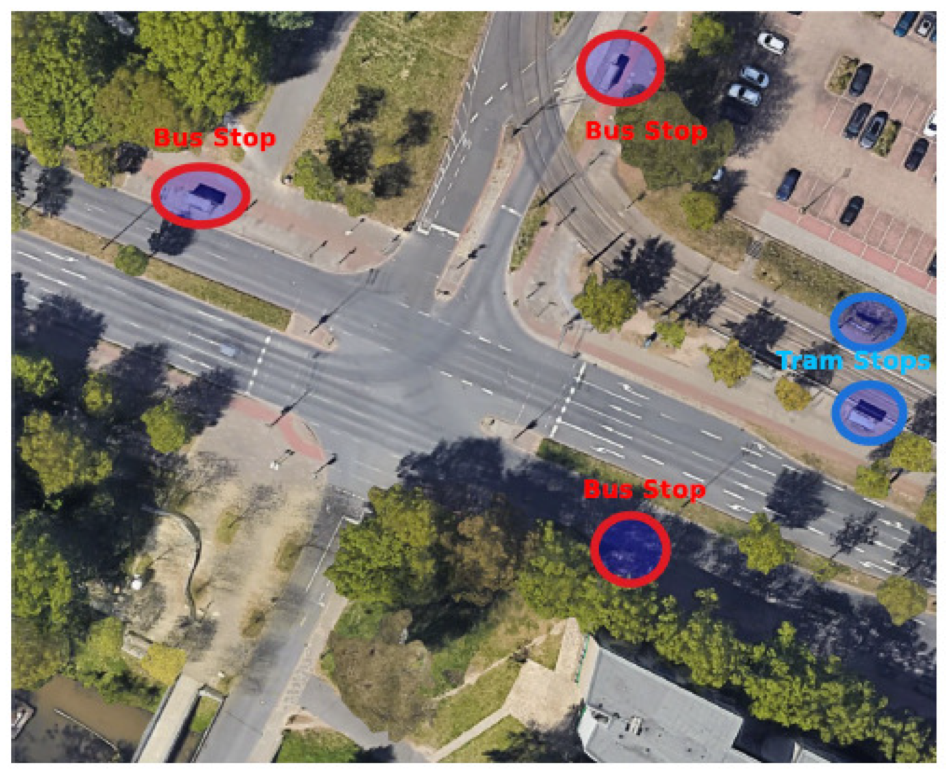
Figure 2.
Distribution of Congestion Levels.
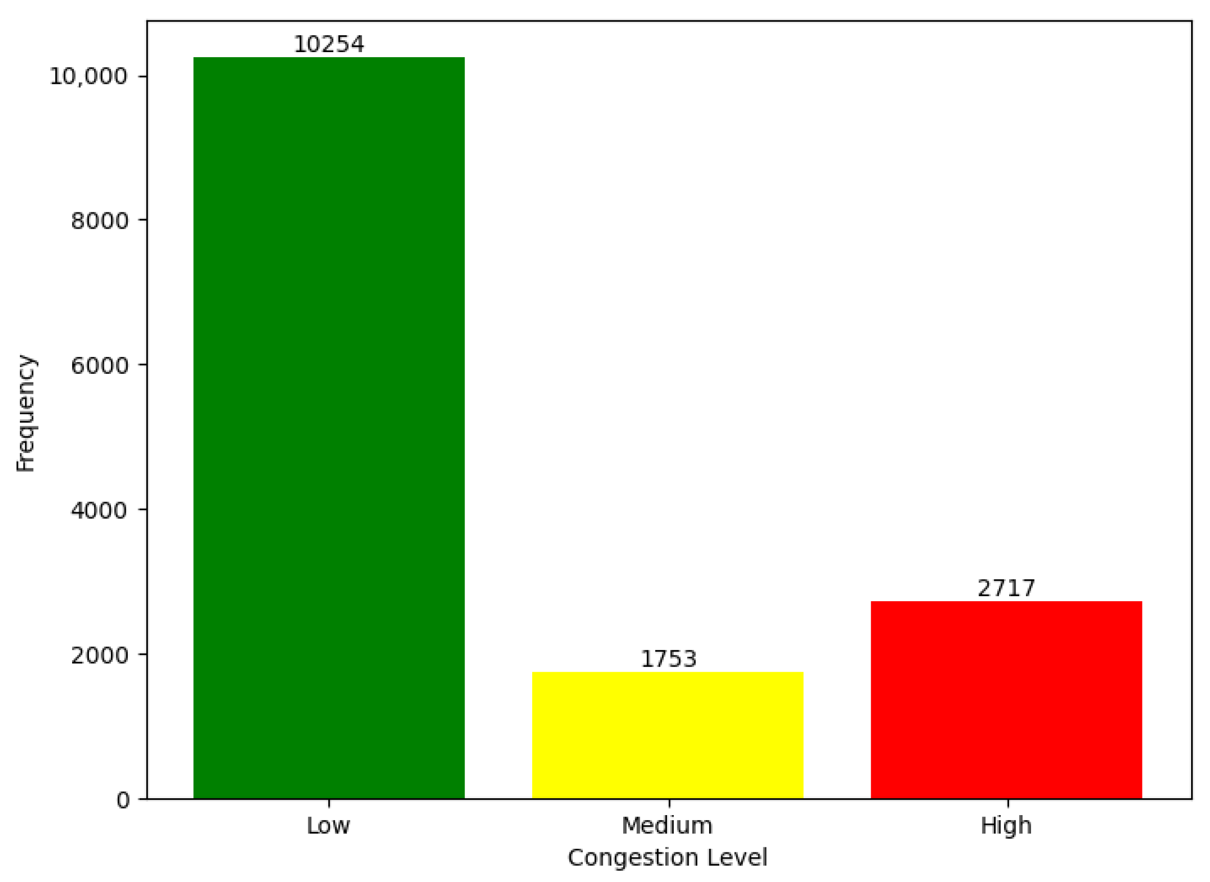
Figure 3.
Distribution of Air Pollutants.
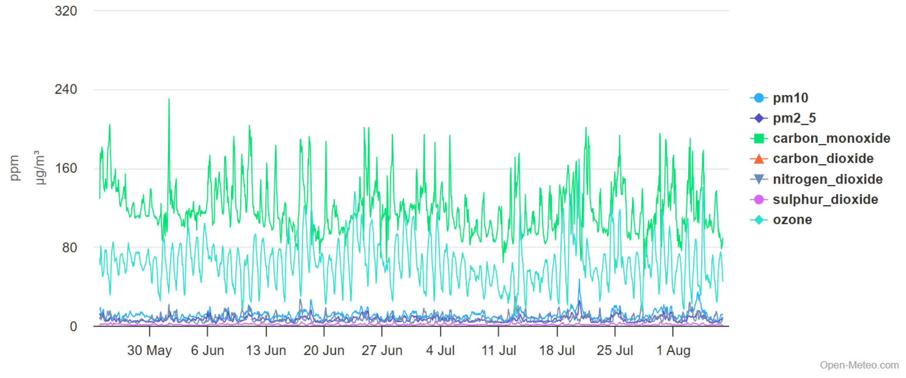
Figure 4.
Wind Direction Mapping to Degrees.
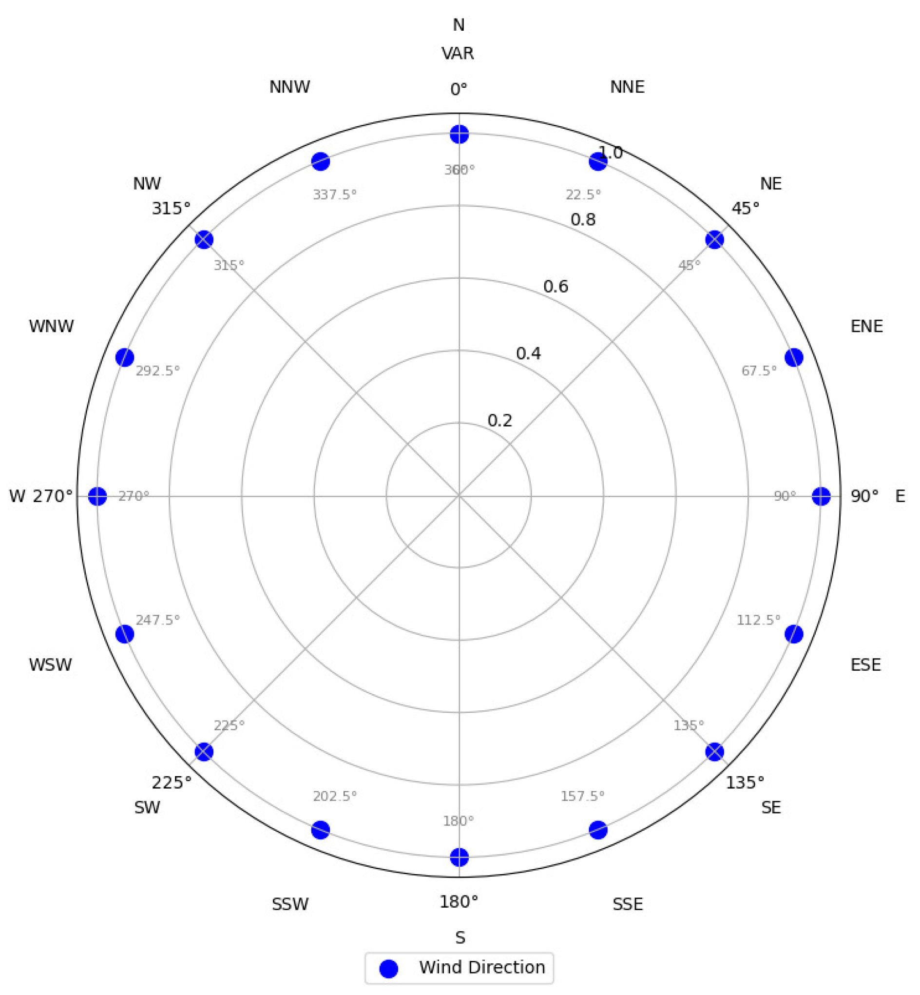
Figure 5.
Relationship Between Vehicle Count and Congestion Level.
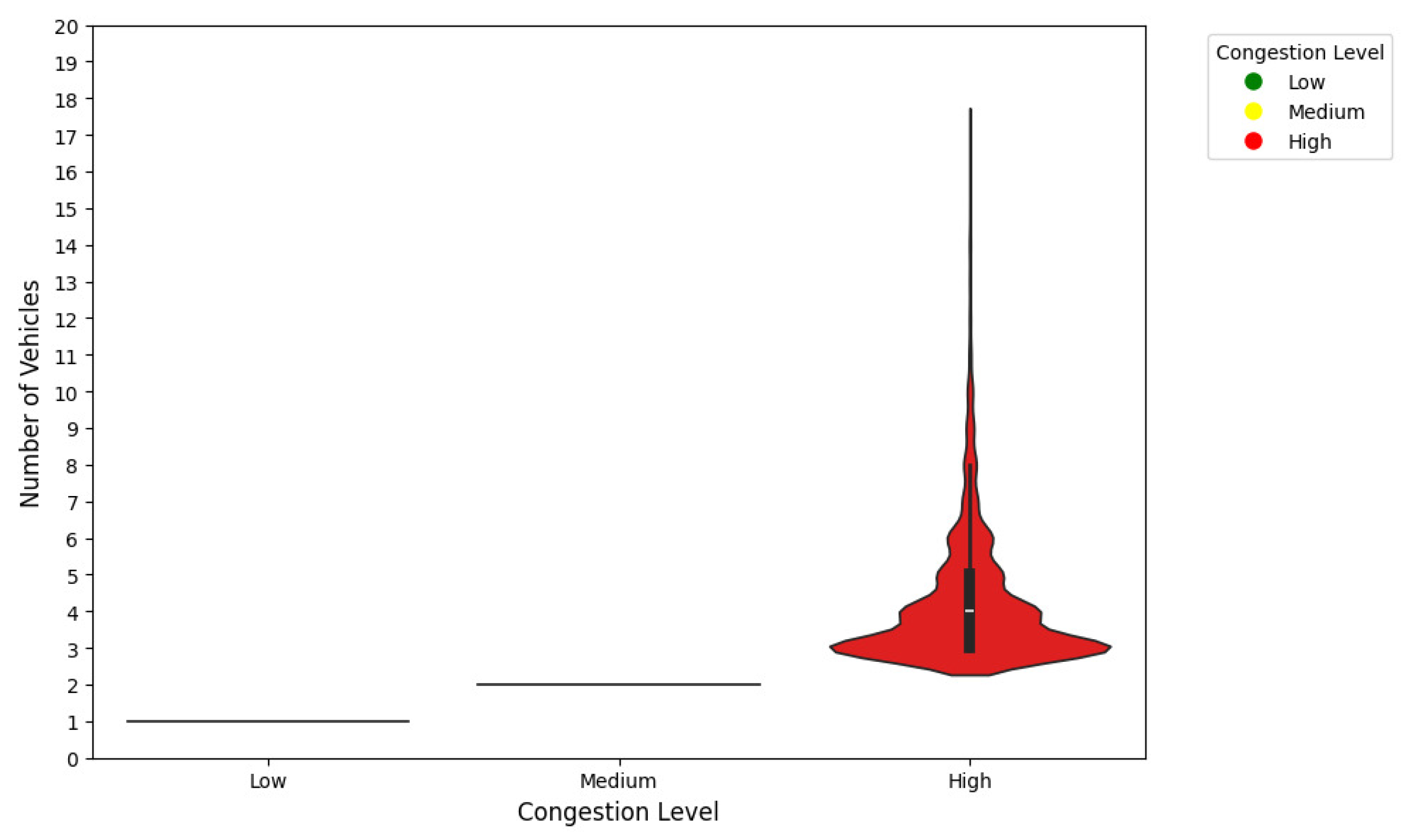
Figure 6.
Hourly Variations in Congestion Incidents.
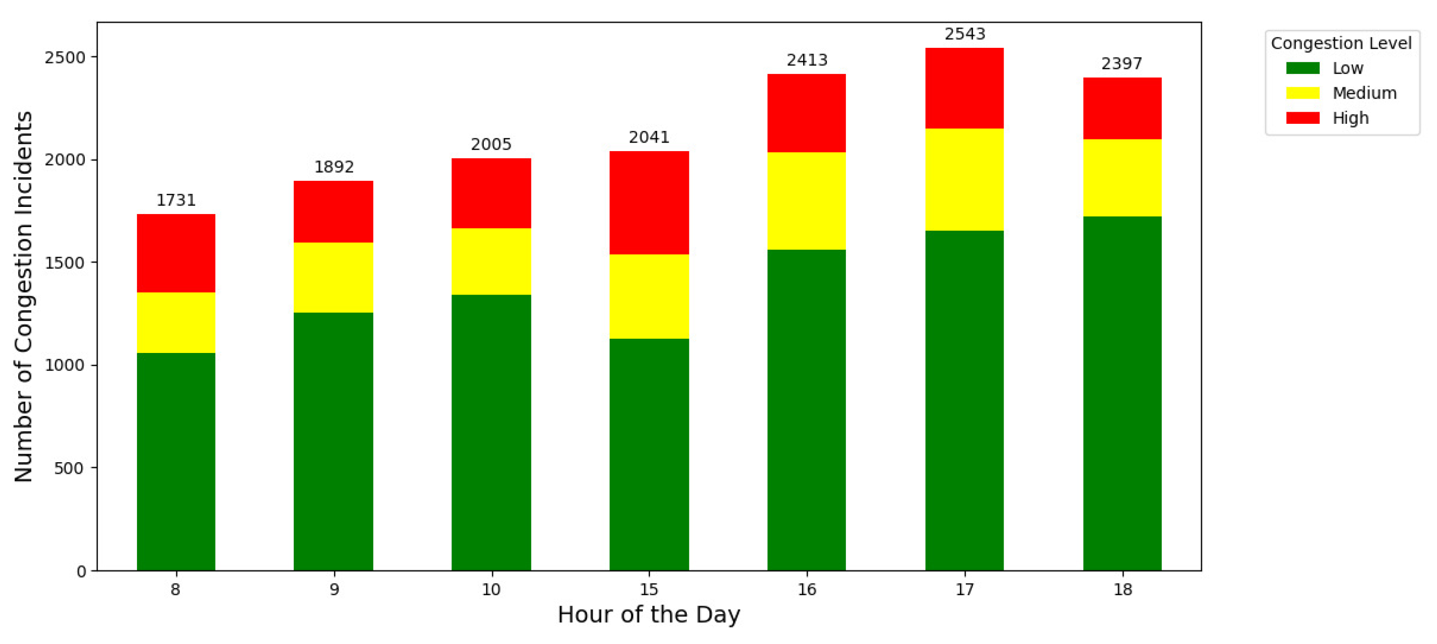
Figure 7.
Weekly Distribution of Congestion Incidents.
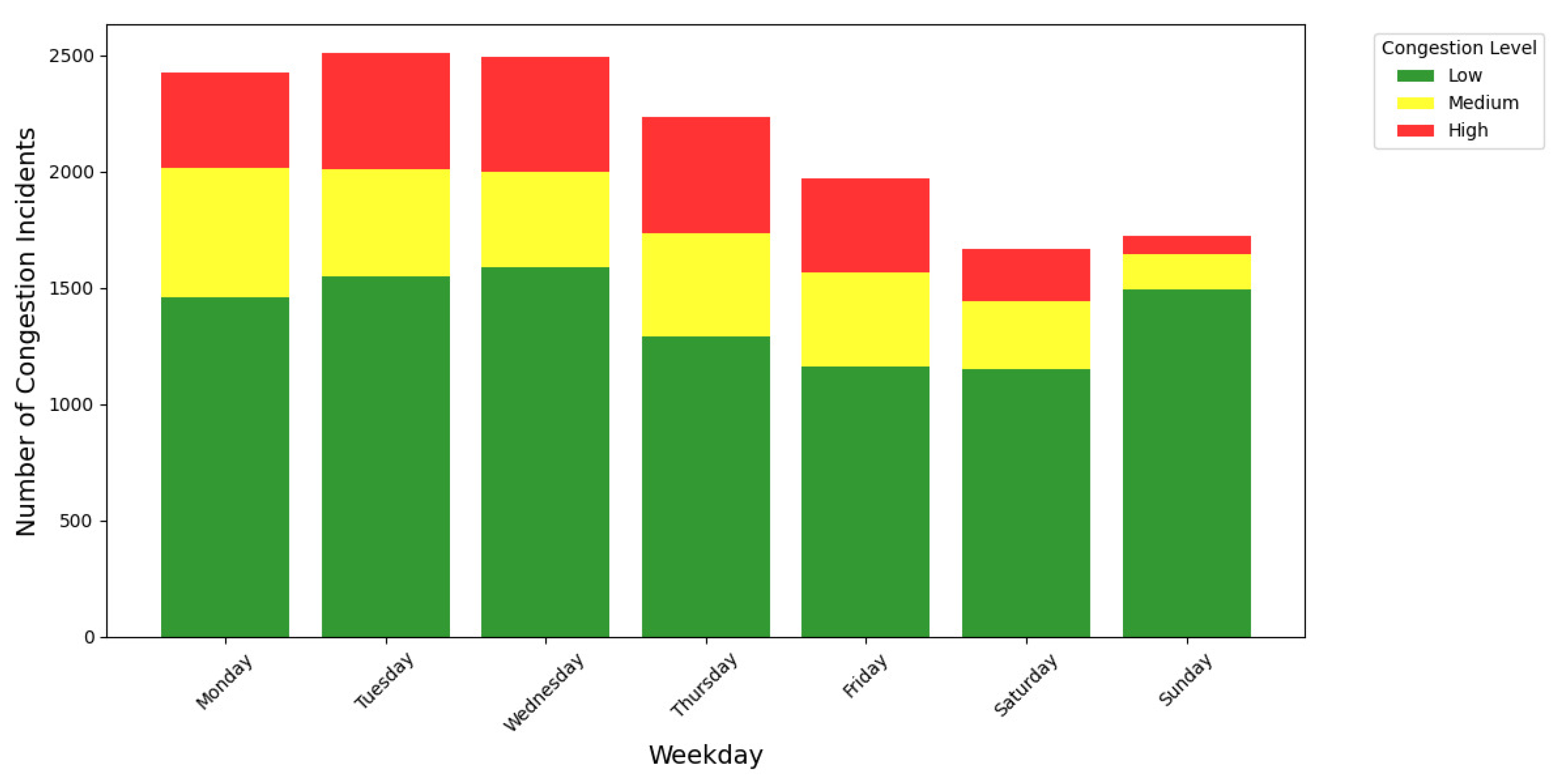
Figure 8.
Direction of Vehicles vs. Congestion Level.
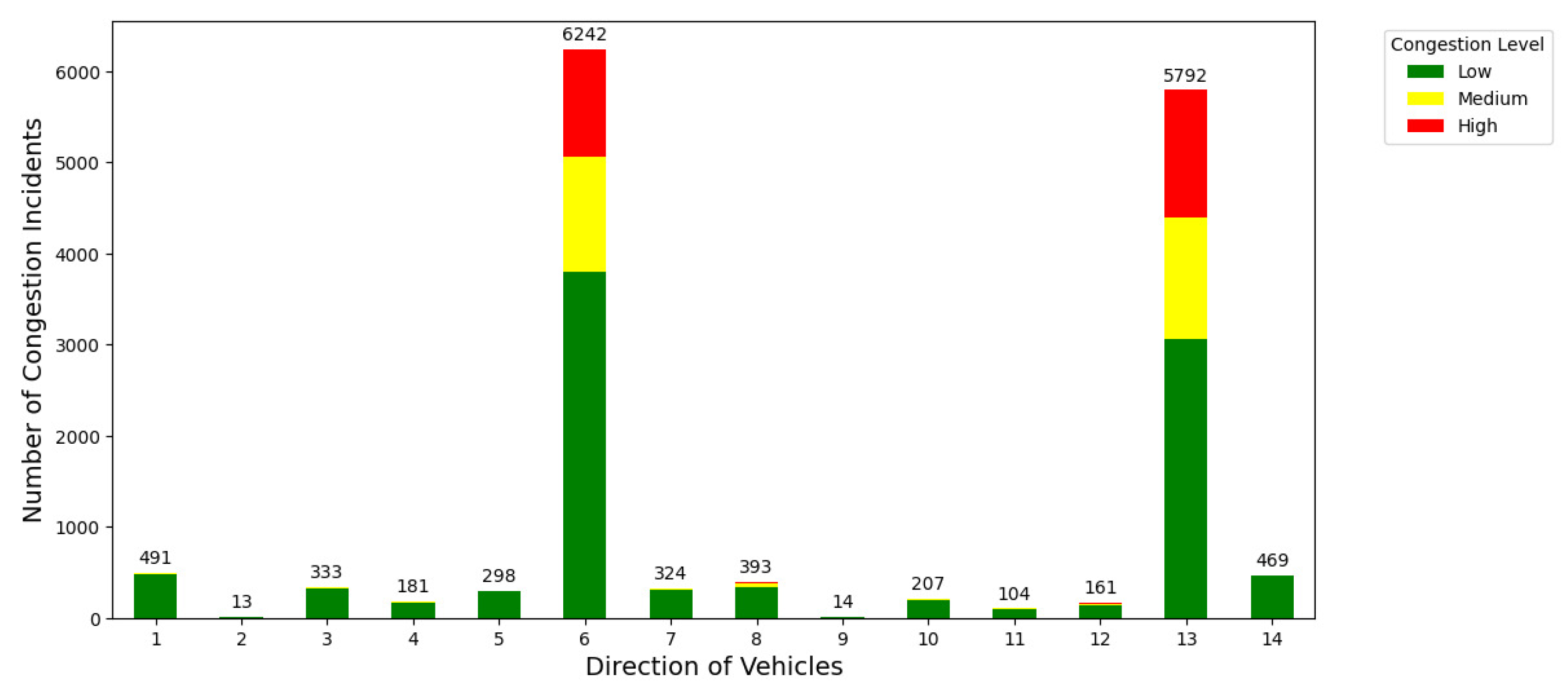
Figure 9.
Monthly Variations in Congestion Incidents.
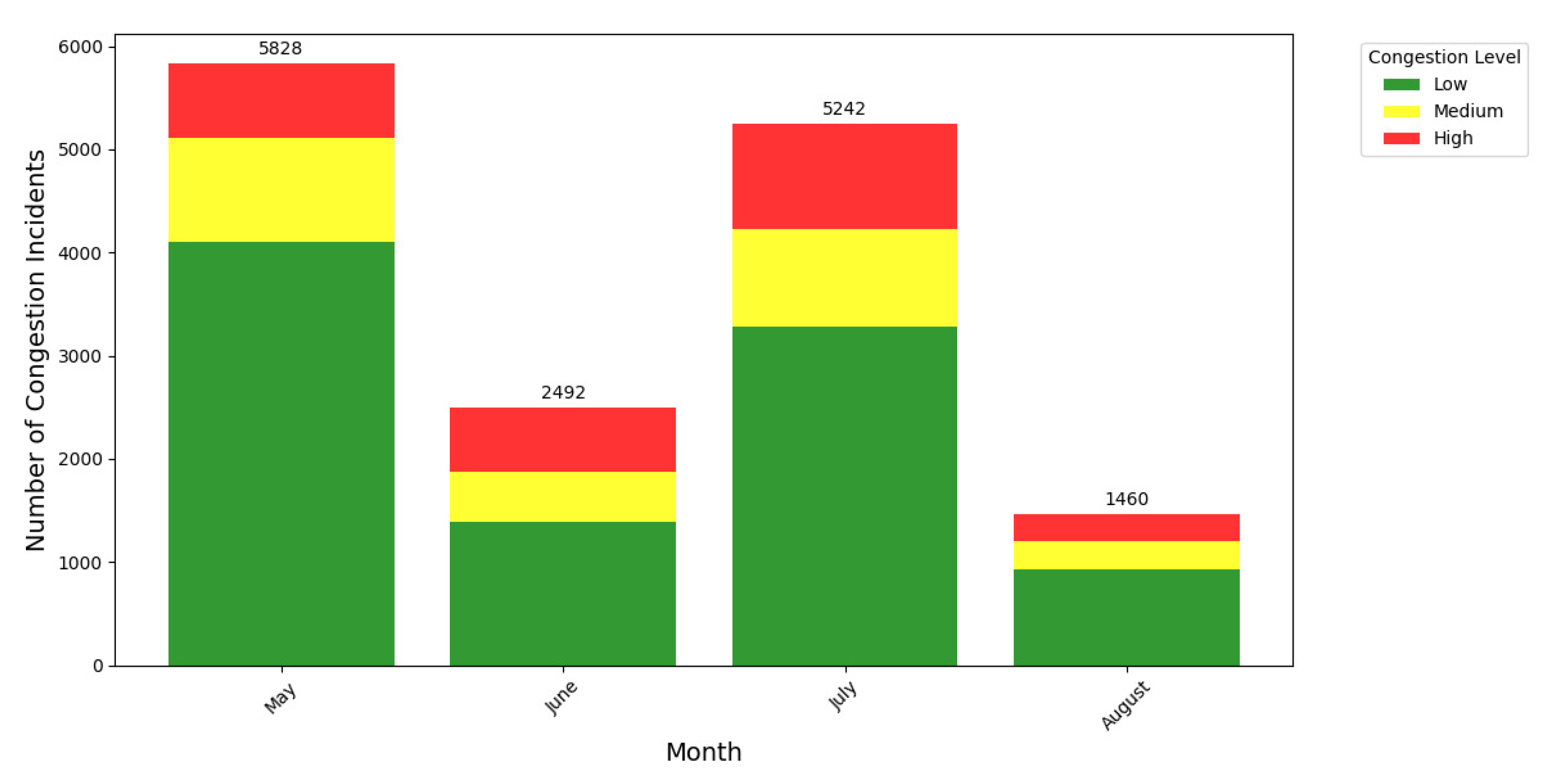
Figure 10.
Comparison of classification algorithm performance.
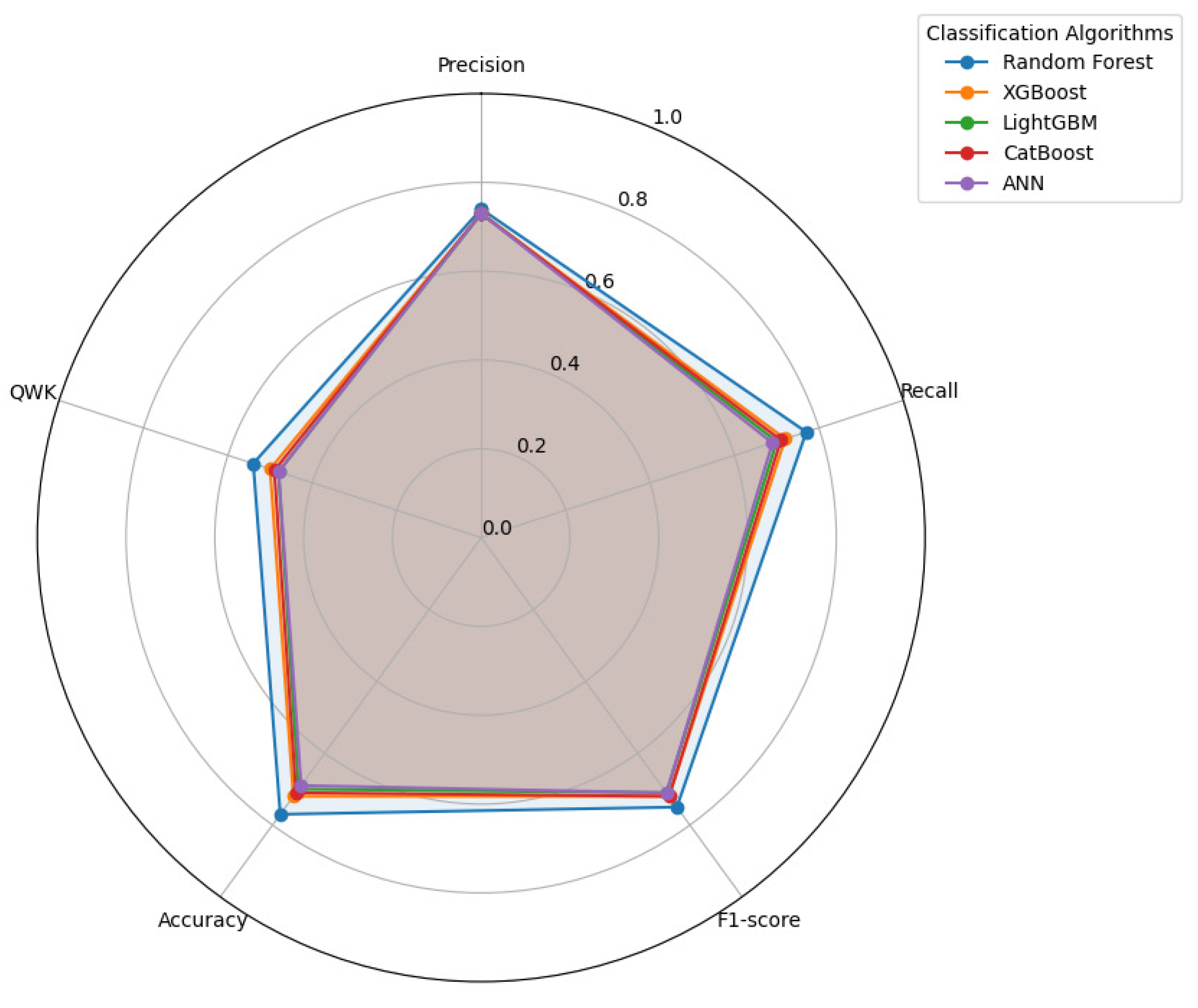
Figure 11.
Impact of Congestion Levels on Air Pollution Trends
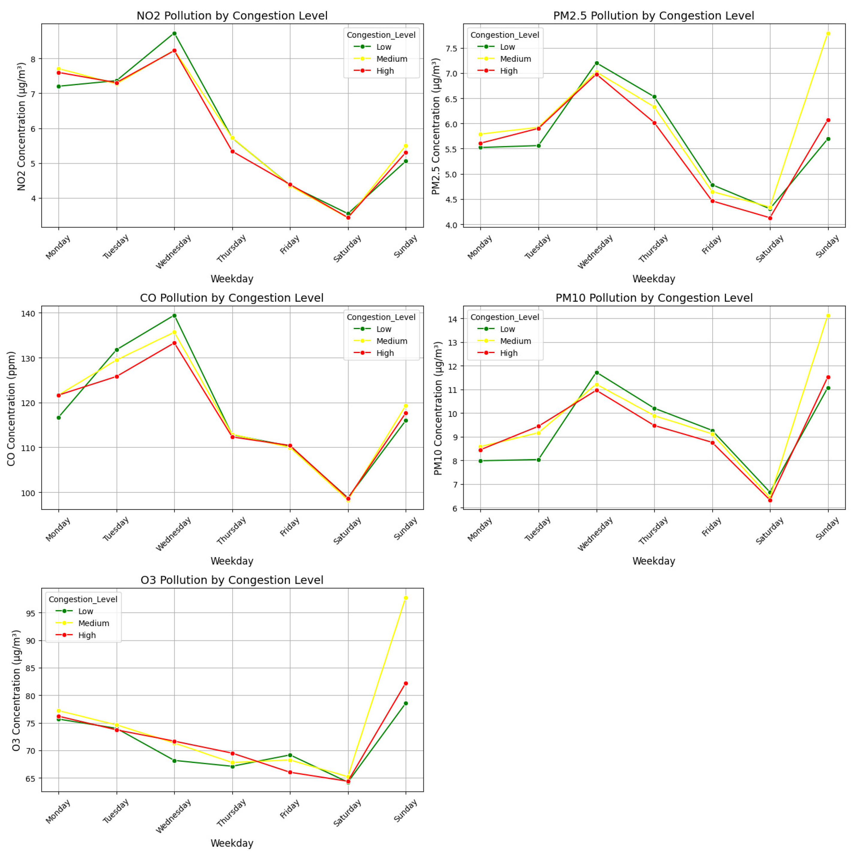

Table 1.
Comparative analysis of machine learning approaches for predicting congestion levels at intersections.
Table 1.
Comparative analysis of machine learning approaches for predicting congestion levels at intersections.
| Reference | Focus | Models/Techniques | Key Findings |
|---|---|---|---|
| [11] | Intersection traffic forecasting | Graph theory, trajectory mining | Real-time analytics with structural time series models. |
| [12] | Urban congestion spot identification | mGCN, DenseNet | Achieved 85.5% accuracy in predicting congestion spots. |
| [13] | Traffic flow prediction | ANFIS, ANFIS-GA | ANFIS-GA achieved R² = 0.9980, surpassing standalone ANFIS. |
| [14] | Multi-intersection traffic modeling | GRU | Demonstrated robust performance even with sparse datasets. |
| [15] | Traffic flow forecasting | LSTM, ARIMA | LSTM outperformed ARIMA in predictive reliability. |
| [16] | Volume prediction | GRU-LSTM, wavelet transform | Achieved 94% accuracy through hybrid noise reduction methods. |
| [17,18] | Hybrid modeling | SARIMA + Bi-LSTM, LSTM + PSO | Achieved low RMSE and high prediction accuracy across test cases. |
| [19,20] | Real-time management frameworks | STNPP, GRU + V2I communication | Effective in reducing congestion and optimizing travel times. |
| [21,22] | Bayesian and ensemble approaches | BCNN, MLP | High regression accuracy; robust multi-lane intersection predictions. |
| [23,24] | Time-series and stacking methods | SARIMA, KNN + Elman NN | Offered computationally efficient and scalable solutions. |
| [25,26,27] | IoT and directed networks | LightGBM, DSAM, LSTM | Reliable congestion management for urban planning and traffic optimization. |
| Current Work | Congestion level prediction at intersections | RF, XGBoost, LightGBM, CatBoost, ANN | Achieved perfect F1 and QWK scores using CN+ dataset with advanced feature selection (DIFS). |
Table 2.
Sample values of weather-related attributes before transformation.
| Temperature | Dew Point | Humidity | Wind Speed | Wind Gust | Pressure |
|---|---|---|---|---|---|
| 61 °F | 48 °F | 63 % | 15 mph | 0 mph | 29.71 in |
| 61 °F | 48 °F | 63 % | 15 mph | 0 mph | 29.71 in |
| 61 °F | 48 °F | 63 % | 15 mph | 0 mph | 29.71 in |
| 61 °F | 48 °F | 63 % | 15 mph | 0 mph | 29.71 in |
| 61 °F | 48 °F | 63 % | 15 mph | 0 mph | 29.71 in |
Table 3.
Sample values of weather-related attributes after transformation.
| Temperature | Dew Point | Humidity | Wind Speed | Wind Gust | Pressure |
|---|---|---|---|---|---|
| 61.0 | 48.0 | 63.0 | 15.0 | 0.0 | 29.71 |
| 61.0 | 48.0 | 63.0 | 15.0 | 0.0 | 29.71 |
| 61.0 | 48.0 | 63.0 | 15.0 | 0.0 | 29.71 |
| 61.0 | 48.0 | 63.0 | 15.0 | 0.0 | 29.71 |
| 61.0 | 48.0 | 63.0 | 15.0 | 0.0 | 29.71 |
Table 4.
Feature importance scores and selection results from the Dual DIFS method.
| Feature | Importance (RF) | Score (Chi2) | Top 25 RF | Top 25 Chi2 | Selected (Final Features) |
|---|---|---|---|---|---|
| Second | 0.149726 | 1.393803 | True | True | True |
| Lane_Capacity | 0.135371 | 625.745138 | True | True | True |
| Minute | 0.128438 | 0.537253 | True | True | True |
| Rolling_Avg_Cong. | 0.115735 | 222.695906 | True | True | True |
| vc_ratio | 0.083693 | 219.885640 | True | True | True |
| Previous_Cong. | 0.074941 | 118.899532 | True | True | True |
| Direction | 0.074234 | 51.890878 | True | True | True |
| Number | 0.037306 | 31.259874 | True | True | True |
| Type | 0.021417 | 1161.434540 | True | True | True |
| o3 | 0.017822 | 1.313062 | True | True | True |
| no2 | 0.015387 | 0.417706 | True | True | True |
| pm2_5 | 0.015247 | 1.012076 | True | True | True |
| so2 | 0.014297 | 1.831040 | True | True | True |
| Temperature | 0.009806 | 7.999304 | True | True | True |
| Day | 0.009368 | 15.255901 | True | True | True |
| Humidity | 0.009286 | 8.865574 | True | True | True |
| Hour | 0.009038 | 14.022089 | True | True | True |
| Wind | 0.009033 | 5.855798 | True | True | True |
| Wind Speed | 0.008898 | 5.567105 | True | True | True |
| Weekday | 0.008526 | 40.147760 | True | True | True |
| Dew Point | 0.007091 | 1.925835 | True | True | True |
| Pressure | 0.007571 | 5.446331 | True | True | True |
| Month | 0.003691 | 8.535287 | True | True | True |
| pm10 | 0.015471 | 0.237498 | True | False | False |
| co | 0.014222 | 0.070474 | True | False | False |
Table 5.
Summary of classification results across different models.
| Class | Precision | Recall | F1-score | Accuracy | QWK Score | Support | Runtime (s) |
|---|---|---|---|---|---|---|---|
| Random Forest (RF) | |||||||
| Low | 0.84 | 0.91 | 0.87 | - | - | 3584 | - |
| Medium | 0.20 | 0.09 | 0.13 | - | - | 518 | - |
| High | 0.60 | 0.61 | 0.60 | - | - | 712 | - |
| Overall | 0.74 | 0.77 | 0.75 | 0.77 | 0.54 | 4814 | 0.081507 |
| XGBoost | |||||||
| Low | 0.85 | 0.82 | 0.84 | - | - | 3584 | - |
| Medium | 0.13 | 0.14 | 0.13 | - | - | 518 | - |
| High | 0.54 | 0.61 | 0.57 | - | - | 712 | - |
| Overall | 0.73 | 0.72 | 0.72 | 0.72 | 0.50 | 4814 | 0.579527 |
| LightGBM | |||||||
| Low | 0.85 | 0.80 | 0.82 | - | - | 3584 | - |
| Medium | 0.14 | 0.17 | 0.15 | - | - | 518 | - |
| High | 0.53 | 0.60 | 0.56 | - | - | 712 | - |
| Overall | 0.73 | 0.70 | 0.71 | 0.70 | 0.48 | 4814 | 6.460226 |
| CatBoost | |||||||
| Low | 0.85 | 0.81 | 0.83 | - | - | 3584 | - |
| Medium | 0.14 | 0.16 | 0.15 | - | - | 518 | - |
| High | 0.54 | 0.60 | 0.57 | - | - | 712 | - |
| Overall | 0.73 | 0.71 | 0.72 | 0.71 | 0.49 | 4814 | 0.376003 |
| Artificial Neural Network (ANN) | |||||||
| Low | 0.85 | 0.78 | 0.82 | - | - | 3584 | - |
| Medium | 0.15 | 0.25 | 0.19 | - | - | 518 | - |
| High | 0.57 | 0.54 | 0.55 | - | - | 712 | - |
| Overall | 0.73 | 0.69 | 0.71 | 0.69 | 0.48 | 4814 | 314.791580 |
Disclaimer/Publisher’s Note: The statements, opinions and data contained in all publications are solely those of the individual author(s) and contributor(s) and not of MDPI and/or the editor(s). MDPI and/or the editor(s) disclaim responsibility for any injury to people or property resulting from any ideas, methods, instructions or products referred to in the content. |
© 2025 by the authors. Licensee MDPI, Basel, Switzerland. This article is an open access article distributed under the terms and conditions of the Creative Commons Attribution (CC BY) license (http://creativecommons.org/licenses/by/4.0/).
Copyright: This open access article is published under a Creative Commons CC BY 4.0 license, which permit the free download, distribution, and reuse, provided that the author and preprint are cited in any reuse.


