Submitted:
05 January 2025
Posted:
06 January 2025
You are already at the latest version
Abstract
In this paper, we prove the Jacod-Yor Theorem for sigma martingales, a class of processes that generalize local martingales and play a pivotal role in financial mathematics. While the Jacod-Yor Theorem has been extensively studied for \( L^2 \)-martingales, martingales, and local martingales, no prior version exists for sigma martingales. Our result establishes the connection between sigma martingales and their martingale representation properties, addressing a critical gap in the literature. As an application, we prove the Second Fundamental Theorem of Asset Pricing for markets where price processes are modeled as sigma martingales.
Keywords:
sigma martingales
; predictable representation property
; Jacod-Yor Theorem
; financial mathematics
; fundamental theorem of asset pricing
MSC: 60H05; 91G30; 60G44; 60G07; 60H30
1. Introduction
The question of determining criteria for a class of processes to be representable as a stochastic integral with respect to a given semimartingale X is fundamental to many applications, particularly in modeling, risk management, and decision-making frameworks. For example, martingale representation theorems enable the expression of portfolio wealth in self-financing trading strategies, directly linking the hedgeability of a claim to its representation as a stochastic integral. Beyond finance, these theorems are indispensable in filtering theory for constructing optimal filters for stochastic signals and in stochastic control for characterizing solutions to stochastic optimal control problems.
Most commonly, the martingale representation theorem is studied in the context of Brownian motion. Originally developed by Itô [16], the theory was extended to square-integrable martingales by Kunita and Watanabe [23] and by Davis and Varaiya [5]. Occasionally, representation theorems are also developed for processes other than Brownian motion such as Possion processes ([22] or Lévy processes ([2,34]).
For local martingales, representation theory is notably sparse, with only a few significant contributions, such as [4,9,24]. Many of these works depend on the Jacod–Yor Theorem, introduced by Jacod and Yor [18], which provides necessary and sufficient conditions for the existence of a martingale representation. While this theorem has been extensively studied for -martingales and, in some cases, local martingales, it has not been extended to sigma martingales.
No general martingale representation theorem exists for sigma martingales. In particular, the Jacod–Yor Theorem has not been established for this class of processes. Karandikar and Rao [20] explicitly acknowledge this shortfall:
"To the best of our knowledge, the martingale representation property in the framework of sigma martingales is not available in the literature. Indeed, most treatments deal with square-integrable martingales where the notion of orthogonality of martingales is available, which simplifies the treatment."
Sigma martingales generalize local martingales and are particularly important in financial mathematics. For example, the First Fundamental Theorem of Asset Pricing (FTAP) asserts the existence of an equivalent sigma martingale measure under the condition of No Lunch with Vanishing Risk (NFLVR), as shown by Delbaen and Schachermayer [7]. This result states that, under certain no-arbitrage conditions, discounted price processes are sigma martingales.
The lack of a martingale representation theory for sigma martingales also affects the Second Fundamental Theorem of Asset Pricing (Second FTAP), which concerns market completeness. The classical Second FTAP, attributed to Harrison et al. [12,13,14], is limited to cases where discounted price processes are martingales or local martingales. While versions of the Second FTAP for sigma martingales are presented in [37] and [20], these works deviate from the economically justified approaches commonly associated with the First FTAP.
This paper aims to fill these gaps by providing a version of the Jacod–Yor Theorem for sigma martingales. As an application, we prove the Second Fundamental Theorem of Asset Pricing in a general form, thereby laying the foundation for a unified theory that bridges sigma martingales, their representation properties, and their role in financial mathematics.
2. Definitions and Main Theorems
Sigma martingales were first introduced as processes "de la classe ()" in [3] and were later formalized in [10]. They arise naturally in financial mathematics, as any process that can be represented as a stochastic integral with respect to a local martingale is necessarily a sigma martingale.
There are several equivalent definitions of sigma martingales. Our definition aligns with that of Goll and Kallsen [11]. Different definitions are used by Jacod and Shiryaev [19], Protter [35], and Delbaen and Schachermayer [7]. Nevertheless, they are all equivalent, as is shown in Theorem 1.
Definition 1.
Let denote the predictable σ-algebra.
- A one-dimensional semimartingale S is called a sigma martingale if there exists a sequence of predictable sets , satisfying for all n, and . Additionally, for any , the process S
- A d
- The vector space of all d .
We recall that denotes the space of -martingales (see Appendix A for details).
The following theorem provides multiple equivalent characterizations of sigma martingales.
Theorem 1 (Characterization of Sigma Martingales)
Let be a d-dimensional semimartingale. The following are equivalent:
- The process X is a sigma martingale.
- There exists a strictly positive predictable process H and an -martingale such that
- There exists a local martingale M = (M1, …, Md) H = (H1, …, Hd)
- There exists a sequence Dn ⊂ Dn ⊂ Dn+1, Dn = Ω × + n ≥ 1, • X
- There exists a sequenceDn ⊂ Dn ⊂ such that Dn⊂ Dn+1, Dn = Ω × +, n ≥ 1, •X
The predictable representation property (PRP) is usually defined for -martingales; see, for example, [35]. Generalizations exist for local martingales as in [15,37]. We extend this concept further to sigma martingales.
Definition 2. For , define:
We say that Xhas the predictable representation property (PRP) if
The PRP is fundamental in applications like mathematical finance, where it enables us to express contingent claims or wealth processes in terms of integrals with respect to a sigma martingale. This property is also central to the Jacod-Yor Theorem for sigma martingales.
Remark 1. The set depends on the probability measure . However, for the sake of simplicity, we only write instead of .
The importance of orthogonality in stochastic analysis traces back to foundational work by P. A. Meyer in the 1960s. In his seminal papers [30,31], Meyer laid the groundwork for understanding martingales using Hilbert-space methods. This perspective was further developed by Itô, Motoo and Kunita [17,23,32], who demonstrated that the space of -martingales could be treated as a Hilbert space. These techniques and tools allowed for significant advancements in the theory of stochastic analysis.
Inspired by this classical notion of orthogonality, we extend the concept to sigma martingales.
Definition 3. Let . We say a process is orthogonal to X if , and we write . Furthermore, we define the set of all processes orthogonal to X as
Remark 2. Clearly, contains all constant processes and for, by partial integration, two sigma martingales are orthogonal if and only if .
Definition 4. Let . Then denotes the sets of all probability measures on such that X is a sigma martingale under . A measure is extremal if, for any and such that , we have .
The main result of this paper is a generalization of the classical Jacod-Yor Theorem to sigma martingales.
Theorem 2 (Jacod-Yor Theorem for Sigma Martingales).
Let . The following are equivalent:
- The process X has the predictable representation property.
- The set only contains the constant processes.
- For any with , we have .
- The probability measure is an extremal point of .
As a classical martingale representation theorem, the Jacod-Yor Theorem has multiple applications. As probably the most popular one, we are going to prove the Second Fundamental Theorem of Asset Pricing for unbounded stochastic processes for a market that satisfies NFLVR. By the First Fundamental Theorem of Asset Pricing [7], we can assume that the discounted price processes are sigma martingales with respect to to some equivalent probability measure.
Our definition of the financial market is essentially the same as in [8] and [7]. For simplicity, we assume discounted processes under an equivalent sigma martingale measure. These simplifications can be justified via the First Fundamental Theorem of Asset Pricing and basic results about general markets. For a general derivation of that setting, starting from a non-discounted setup with a real-world probability measure, we refer to [38].
We consider a financial market consisting of tradeable securities whose price processes are represented by the -dimensional process adapted to the filtration . We make the following assumptions:
- The processes are sigma martingales for all .
- The filtration satisfies the usual conditions, and the σ-algebra is trivial; that is, implies or .
Definition 5.
- We call a -dimensional process a trading strategy.
-
The wealth process of the investor is defined aswhere represents the number of the i-th security that the investor holds in their portfolio at t.
- A trading strategy is called self-financing if the wealth process satisfies
- A self-financing strategy is called admissible if there exists an such thatfor the corresponding wealth process V.
- A contingent claim X settled at time T is a non-negative -measurable, integrable random variable.
We now turn to the Second Fundamental Theorem of Asset Pricing. In the case of finitely many assets, a version of this theorem was first proved for the discrete-time setting in [12]. The proof for the continuous-time case followed in [13,14], but Sigrid Müller showed in [33] that the statement in a higher-dimensional case is not valid for the componentwise stochastic integral without additional assumptions. However, one can bypass the additional assumptions by not restricting the class to the componentwise-integrable integrands, as shown in [27] and [28]. In all these publications, however, a probability measure is assumed under which the process is a local martingale and not just a sigma martingale.
Theorem 3 (Second Fundamental Theorem of Asset Pricing).
Let (with ) be a -dimensional sigma martingale under . The following are equivalent:
- The market is complete, that means for each contingent claim X, there exists an admissible self-financing such that S (•S)T = X
- M φ ∈ L(S)
- X ∈ φ ∈ L(S)
- X ∈ φ ∈ L(S)
- Q S = .
Proof. (i) ⇒ (ii). Assume the market is complete. Let M be a uniformly integrable martingale. Then is a submartingale with . By the Krickeberg (or Doob–Meyer) decomposition, M can be assumed w.l.o.g. nonnegative. Then is a claim. Completeness implies there is a self-financing φ such that S) L1 MT T t ≤ T M = φ •S.
- (iv) ⇔ (v). This follows directly from the Jacod-Yor Theorem (Theorem 2).
- (iv) ⇒ (iii) ⇒ (ii). These inclusions are obvious.
- (ii) ⇒ (i). Finally, if every UI martingale is a true martingale stochastic integral in S, then the model is complete. Indeed, let be any claim. Define , a UI martingale. By (ii), S φ 0 M0 = [X] φ •S (φ•S)T = X X □
Remark 3. In the statement of completeness, we require that any replicating strategy S L1- T X T .
Some authors ensure the true martingale property by requiring that all replicating strategies be bounded (or that φ be bounded), which trivially forces S) (φ •S)
For an example of a market that admits a hedging strategy replicating a claim but lacks a martingale hedging strategy and, consequently, market completeness, refer to Example 7.3 in [37].
3. Proof of the Jacod-Yor Theorem for Sigma Martingales
By , we denote the space d-dimensional martingales, by the space of bounded d-dimensional martingales, and by the space of d-dimensional local martingales. A subscript 0 as in will further indicate that the process starts in 0, that is almost surely for all .
Lemma 1. Let and let Y be locally in . Then we have .
Proof.
Let Y be locally in . That means there exists an increasing sequence of stopping times , tending to infinity, such that there are with X for all n ∈ . T0: = 0 H: Hn , H ∈ L(X) Y = H•X Y = H • X Y ∈
(X) □
Definition 6. Let V be a vector space of stochastic processes. We say V is stable if implies .
In the literature, it is often required that a stable subspace is also closed. In such a case, we will speak of a stable, closed vector space.
Lemma 2. Let . Then, is a stable and closed subspace of .
Proof.
Because of the linearity of the stochastic integral and since is a vector space, is also a vector space. We have for X ∈ 1(X) T
where
Hence (H•X)T ∈ (X).
(H•X)T ∈ 1 1(X)
We still have to show the closedness. For , we put
I1(X) {H ∈ L(X); {H ∈ L(X);
Lp I1 (X) Now let Hn•X
I1(X)
□
Theorem 4. Let . The following are equivalent:
- The process X has the predictable representation property;
- ;
- ;
- .
Proof. (i) ⇒ (ii).
This is trivial.
- (ii) ⇒ (iii). Let . By Theorem A2, is dense in . Hence, there exists a sequence that converges in to N. By assumption, we have for all n, and from Lemma 2, we know that is closed. Thus, .
- (iii) ⇒ (iv). By Theorem A3, each local martingale is locally in . Hence, by assumption, each local martingale is locally in and, therefore, in . Lemma 1 yields .
- (iv) ⇒ (i). Let . By Theorem 1, there exists a one-dimensional martingale M and a process such that M K ∈ L(X) M = K •X.
and □
The following lemma is often used in connection with Girsanov’s theorem (see, for example, [35] Exercise III.21, [4] Lemma 15.2.1, [19] Proposition 3.8, [21] Lemma 18.16, [25] Lemma 8.9.3, [15] Lemma 12.11, [2] Lemma 5.2.11).
Lemma 3.Suppose a semimartingale M, and let be the Radon-Nikodym derivative with
Then M is a -(local) martingale if and only if is a -(local) martingale.
We are going to investigate a possible generalization to sigma martingale measures.
Lemma 4. Let X be a semimartingale, , the Radon-Nikodym derivative and
- If X is a sigma martingale, then is a -sigma martingale.
- If then X is a -sigma martingale if and only if is a -sigma martingale.
Proof.
First we note that by [35] Theorem IV.25 , it is irrelevant whether we calculate the integral under or . We will therefore only write • •
• X
For any Borel set , we have
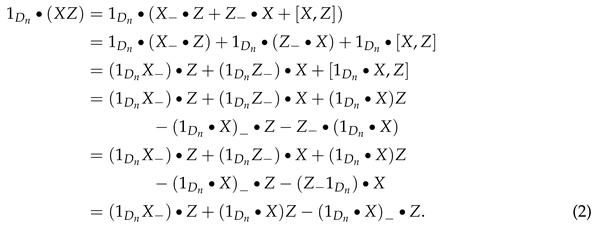
Let X be a -sigma martingale with localizing sequence . By Lemma 3, X) Z
(X-) (•X)-
Z
•(XZ)
XZ XZ
Now let be a -sigma martingale and . Then we have and is given by . Applying the already proven direction yields that is a -sigma martingale. □
Lemma 5. Let and , then there exists a process with for all i and a stochastic process with for all i with
Furthermore, if there exists a stochastic process such that , then we also have .
Proof. By Theorem 1, each can be written as Ni with a strictly positive and
for all i. We set
and obtain H•X = G•N for G = (G1,…,Gd)⊤ Nowweput K: ‖= ‖ ∨ 1and and is a bounded process and thus Ji ∈ L(Xi)for each i. We have
By putting Mi: = Ji•Ni we obtain the desired result.
Now let with . By partial integration, we get
Hence, we obtain
Since
is strictly positive, we also get
Analogously, we obtain
Since all three summands on the right-hand side are sigma martin-
gales. We conclude that ZMi is a sigma martingale as well. □
For the proof of the Jacod-Yor Theorem for sigma martingales, we recall that denotes the space of BMO martingales (see Appendix A).
Theorem 5 ([26] Theorem 4.2.3).
Let X be a normed space with dual space , a subspace M and let , such that
There exists a , such that
- for all ,
- ,
- .
Theorem 6 (Ansel-Stricker)
. A one-sided bounded sigma martingale X is a local martingale. If X is bounded from below (resp. above), it is also a supermartingale (resp. submartingale).
We can now prove the Jacod-Yor Theorem for sigma martingales.
Proof of Theorem 2. (i) ⇒ (ii).
Suppose . By assumption, there exists an such that
Now Lemma 5 yields amartingale M = (M1, …, Md)⊤ and aprocess K = (K1, …, Kd)⊤ with Ki L(Mi) such that
We define
where
Hence, N N Theorem 6, N
Nt ≤ N0. N N Z
(ii) ⇒ (iii). Let with . Define
Since X is a -sigma martingale, is a -sigma martingale by Lemma 4. By assumption, Z is constant. Hence, we have .
(iii) ⇒ (iv).
Let and such that . Clearly, . By assumption, we have . Similarly, . Thus, is an extremal point in .
(iv) ⇒ (i).
By Theorem 4, it suffices to show that .
Suppose this is not the case. Then, by Lemma 2, is a stable closed subspace of , and there exists an element , , such that
By Theorem 5, there exists a bounded linear functional with and .
By Theorem A5, φ can be represented as
where .
Thus, for all . Since is stable, we have
By Theorem A4, M is locally bounded. Thus, there exists a sequence of stopping times such that . Define
where is a constant larger than .
Clearly, all and are bounded martingales. Define probability measures by and .
Since and , we conclude with (3) that is a -sigma martingale. Similarly, is a -sigma martingale. By Lemma 4, .
Because , we get, by assumption, . Thus,
which implies for all n. Taking , we get , and hence .
Therefore, no process can exist with . Thus, follows. □
Appendix A. Martingale Spaces
Definition A1. For M a martingale and , write
Here denotes the norm in . Then is the space of martingales such that
Theorem A1. Let . Then, a càdlàg process X is locally uniformly bounded in if and only if is locally uniformly bounded in .
Theorem A2 ([4] Theorem 10.1.7).
The space of bounded martingales (and hence for any ) is dense in .
Theorem A3 ([15] Theorem 7.30)
Let . Then M is locally in .
The definition of the given here is taken from [35]. A similar presentation can also be found in [4,15,29], which use equivalent definitions.
Definition A2. Let . We say , if there exists a constant c such that for any stopping time T we have
The smallest such c is defined to be the
-Norm of M, and it is written . If the constant c does not exist, or if M is not in , then we set .
For the definition above, we use the convention .
Theorem A4 ([4] Lemma A.8.7 and Lemma A.8.5).
Each -martingale is locally bounded, and each bounded martingale is element of .
Theorem A5 ([4] Theorem A.8.14).
Any continuous linear function can be written for some .
References
- Ansel, J.-P., and Stricker, C., Couverture des actifs contingents et prix maximum, Annales de l’institut Henri Poincaré (B) Probabilités et Statistiques, vol. 30, Gauthier-Villars, 1994, pp. 303–315. 1277002.
- Applebaum, D., Lévy processes and stochastic calculus (cambridge studies in advanced mathematics), 2nd ed., Cambridge University Press, 2009. 2512800.
- Chou, C.-S., Caracterisation d’une classe de semimartingales, Séminaire de Probabilités XIII, Springer, 1979, pp. 250–252. 0544798.
- Cohen, S. N., and Elliott, R. J., Stochastic calculus and applications, Probability and Its Applications, Springer New York, 2015. 3443368.
- Davis, M. H. A., and Varaiya, P., The multiplicity of an increasing family of σ-fields, The Annals of Probability (1974), 958–963. 0370754.
- De Donno, M., and Pratelli, M., On a lemma by Ansel and Stricker, Séminaire de Probabilités XL, Springer, 2007, pp. 411–414. 2409019.
- Delbaen, F., and Schachermayer, W., The fundamental theorem of asset pricing for unbounded stochastic processes, Mathematische Annalen312(1998), no. 2, 215–250. 1671792. [CrossRef]
- Delbaen, F., and Schachermayer, W., A general version of the fundamental theorem of asset pricing, Mathematische Annalen 300 (1994), no. 1, 463–520. 1304434.
- Dellacherie, C., and Meyer, P.-A., Probabilities and potential, North-Holland Mathematics Studies, Hermann, Amsterdam, 1978. 0521810.
- Émery, M., Compensation de processus vf non localement intégrables, Séminaire de Probabilités XIV 1978/79, Springer, 1980, pp. 152–160. 607308.
- Goll, T., and Kallsen, J., A complete explicit solution to the log-optimal portfolio problem, The Annals of Applied Probability 13 (2003), no. 2, 774–799. 1970280. [CrossRef]
- Harrison, J. M., and Kreps, D. M., Martingales and arbitrage in multiperiod securities markets, Journal of Economic theory 20 (1979), no. 3, 381–408. 544800.
- Harrison, J. M., and Pliska, S. R., Martingales and stochastic integrals in the theory of continuous trading, Stochastic processes and their applications11(1981), no. 3, 215–260. 622165A stochastic calculus model of continuous trading: Complete markets, Stochastic Processes and their Applications 15 (1983), no. 3, 313–316. 711188. [CrossRef]
- A stochastic calculus model of continuous trading: Complete markets, Stochastic Processes and their Applications 15 (1983), no.3,313–316.711188. [CrossRef]
- He, S. W., Wang, J. G., and Yan, J. A., Semimartingale theory and stochastic calculus, Kexue Chubanshe (Science Press), Beijing; CRC Press, Boca Raton, FL, 1992. 1219534.
- Itô, K., Multiple Wiener integral, Journal of the Mathematical Society of Japan 3 (1951), no. 1, 157–169. 44064. [CrossRef]
- Itô, K., Transformation of markov processes by multiplicative functionals, Ann. Inst. Fourier 15 (1965), no. 1, 15–30. 184282.
- Jacod, J., and Yor, M., Étude des solutions extrémales et représentation intégrale des solutions pour certains problèmes de martingales, Probability Theory and Related Fields 38 (1977), no. 2, 83–125. 445604. [CrossRef]
- Jacod, J., and Shiryaev, A. N., Limit theorems for stochastic processes, second ed., Grundlehren der mathematischen Wissenschaften [Fundamental Principles of Mathematical Sciences], vol. 288, Springer-Verlag, Berlin, 2003. 1943877.
- Karandikar, R. L., and Rao, B. V., On the second fundamental theorem of asset pricing, 2016, pp. Article 5, 57–81. 3619713.
- Kallenberg, O., Foundations of modern probability, 2. ed., Springer, 2002. 1876169.
- Klebaner, F. C., Introduction to stochastic calculus with applications (2nd edition), 2. ed., ICP, 2005. 2160228.
- Kunita, H., and Watanabe, S., On square integrable martingales, Nagoya Mathematical Journal 30 (1967), 209–245. 217856. [CrossRef]
- Kussmaul, A. U., Stochastic integration and generalized martingales, Research Notes in Mathematics, No. 11, Pitman Publishing, London-San Francisco, Calif.-Melbourne, 1977. 488281.
- Kuo, H.-H., Introduction to stochastic integration (universitext), 1. ed., Springer, 2005. 2180429.
- Larsen, R., Functional analysis: an introduction, Pure and applied mathematics, M. Dekker, 1973. 461069.
- Madan, D. B., and Jarrow, R. A., A characterization of complete security markets on a Brownian filtration, Mathematical Finance 1 (1991), no. 3, 31–43. 1214465. [CrossRef]
- italic>Madan, D. B., and Chatelain, M., On componentwise and vector stochastic integration, Mathematical Finance 4 (1994), no. 1, 57–65. 1286706. [CrossRef]
- Medvegyev, P., Stochastic integration theory, Oxford Graduate Texts in Mathematics, OUP Oxford, 2007. 2345169.
- Meyer, P.-A., A decomposition theorem for supermartingales, Illinois Journal of Mathematics6(1962), no. 2, 193–205. 159359Decomposition of supermartingales: The uniqueness theorem, Illinois Journal of Mathematics7(1963), no. 1, 1–17. 144382.
- Decomposition of supermartingales: The uniqueness theorem, Illinois Journal of Mathematics 7 (1963), no.1,1–17. 144382.
- Motoo, M., and Watanabe, S., On a class of additive functionals of Markov processes, Journal of Mathematics of Kyoto University4(1965), no. 3, 429–469. 196808.
- Müller, S. M., On complete securities markets and the martingale property of securities prices, Economics Letters 31 (1989), no. 1, 37–41. 1035110. [CrossRef]
- Nualart, D., and Schoutens, W., Chaotic and predictable representations for lévy processes, Stochastic processes and their applications 90 (2000), no. 1, 109–122. 1787127. [CrossRef]
- Protter, P., Stochastic integration and differential equations: Version 2.1 (stochastic modelling and applied probability), Springer, 2010. 2273672.
- Rudin, W., Real & complex analysis, Mcgraw Hill Higher Education, 1987. 924157.
- Shiryaev, A. N., and Cherny, A., Vector stochastic integrals and the fundamental theorems of asset pricing, Proceedings of the Steklov Institute of Mathematics-Interperiodica Translation 237 (2002), 6–49. 1975582.
- Sohns, M., The general market model with dividends, (2024), Submitted to African Finance Journal.
- Sigma martingales and asimplified proof of the Ansel-Stricker lemma, Preprints, 2025, January, Preprints. Available at: https://doi.org/10.20944/preprints202501.0175.v1. [CrossRef]
| 1 | compare, forexample, [36] Theorem 3.11. |
Disclaimer/Publisher’s Note: The statements, opinions and data contained in all publications are solely those of the individual author(s) and contributor(s) and not of MDPI and/or the editor(s). MDPI and/or the editor(s) disclaim responsibility for any injury to people or property resulting from any ideas, methods, instructions or products referred to in the content. |
© 2025 by the authors. Licensee MDPI, Basel, Switzerland. This article is an open access article distributed under the terms and conditions of the Creative Commons Attribution (CC BY) license (http://creativecommons.org/licenses/by/4.0/).
Copyright: This open access article is published under a Creative Commons CC BY 4.0 license, which permit the free download, distribution, and reuse, provided that the author and preprint are cited in any reuse.


