
Submitted:
26 December 2024
Posted:
27 December 2024
You are already at the latest version
Abstract
The rapid economic growth in recent years has led to a surge in stock market participation, necessitating accurate stock price prediction to mitigate investment risks and maximize returns. However, stock price’s dynamic nature and intrinsic volatility pose significant challenges to traditional statistical and machine learning (ML) models, which often struggle with overfitting, poor robustness, and limited generalization. To address these challenges, this study introduces EvoBagNet, an evolutionary Bagging ensemble learning model specifically designed for robust and high-accuracy stock price prediction. The proposed framework integrates nine state-of-the-art ML techniques, encompassing tree-based methods, neural networks, and both boosting and bagging ensemble approaches, applied to recent datasets from nine prominent IT sector companies. Extensive experimentation was conducted using multiple train-test split ratios to evaluate the scalability and adaptability of the models under diverse scenarios. The performance of EvoBagNet was assessed against six evaluation metrics, revealing its superior accuracy and robustness compared to alternative models. EvoBagNet demonstrated exceptional prediction accuracy across all datasets, achieving performance scores of 97.0%±0.7, 98.3%±0.5, 97.3%±0.8, 97.4%±0.6, 97.0%±1.0, 98.6%±0.4, 98.8%±0.4, 91.7%±1.2, and 98.4%±0.3 for Tech Mahindra, Mindtree, Infosys, Wipro, TCS, Mphasis, L&T Tech, HCL, and Coforge, respectively. These results highlight EvoBagNet’s potential as a powerful tool for stock price forecasting, offering significant implications for informed investment strategies and financial decision-making. This study underscores EvoBagNet’s effectiveness in addressing the limitations of traditional ML models, paving the way for its application in dynamic and high-stakes financial markets.
Keywords:
bagging ensemble learning
; machine learning
; hyper-parameter tuning
; feature selection
; stock prediction
; evolutionary algorithm
1. Introduction
A stock market often known as the equity market comprises several global stock exchanges [1]. It is a snapshot of future growth of the economy as well as the company’s expectations. Buying and selling the shares at the right time increases the capital and generates a good return for investors [2]. As per the Efficient Market Hypothesis (EMH) [3], stock market price imitates total present information. It allows price discovery of shares of corporations and serves as a barometer of the overall economy. Since there is a huge number of stock market participants, one can usually expect fair pricing and a high level of liquidity as the market participants compete for the best price with transparency in transactions [4]. Over the last few years, people have gained more interest in stock trading. The stock market has also changed due to technological advancements and online trading. It is considered a dynamic and chaotic financial system [5] because its behaviour is influenced by unpredictable factors, including investor expectations, political situations in the country, and so on [6]. Stock market data is a non-linear and variable time series data, i.e., a collection of data calculated over time to acquire various activity statuses [7]. This complex financial system involves a wide range of companies and their stocks, as well as price adjustments that vary over time for each company. Stock market prediction is the process of estimating the future value of a company’s commodity or any other financial instrument being traded on the stock exchange. As per [8,9], financial time series data prediction is regarded as a notoriously challenging task for statistics experts and finance. Every investor plans to increase the profit from their investments and decrease the correlated risks [10]. A successful prediction can result in substantial gains for both the seller as well as the buyer and can be carried out by in-depth analysis of past data. As per [11], there are two approaches to stock forecasting. One is fundamental analysis, which depends on business methodology and basic data such as yearly growth rates, expenses, and market position. The second approach is technical analysis, which focuses on historical stock values.
Now a day’s world needs an automated and accurate prediction system. Predicting the stock market in the financial system is difficult but rewarding. Typically, in the stock market, a huge amount of structured and unstructured heterogenous market data is generated. Because of the exponential growth of data in the financial market, it is very complex to analyze it with the traditional statistical models [12]; analysts and researchers tried to solve this problem by applying various statistical approaches but may not produce more accurate results. Finally, they found data mining to be the best solution for dealing with a large volume of structured and unstructured heterogeneous data. With the advancement of Machine Learning approaches, there has been good progress in the automation of the prediction process of the stock market [13,14], but still, there is a scope in the system to produce more accurate results. With the development of technologies like ML, the ability to predict the stock market has improved significantly. In machine learning, the model is trained on past stock data to perform future stock price or stock movement prediction.
In this work, nine popular machine learning (ML) approaches, namely Support Vector Regression (SVR), Random Forest (RF) [15], Lasso Regression, Neural Networks (NN), Extreme Gradient Boosting (XGBoost) [16], Gradient Boosting Regressor (GBR) [17], Decision Tree (DT) [18], Light Gradient Boosting Machine (LGBM) [19], and Categorical Boosting (CatBoost), are applied to predict the future closing prices of leading IT sector stocks. Additionally, six bagging ensemble models are proposed, enhanced through an automatic hyper-parameter tuner based on a fast and effective evolutionary algorithm. Bagging ensemble models are particularly advantageous as they reduce variance, improve model stability, and enhance robustness against overfitting by combining predictions from multiple learners.
Recent data from nine IT sector companies has been collected to conduct the experimental analysis. A feature selection process has been employed to identify the optimal features, and extensive hyperparameter tuning has been conducted to achieve better predictive performance. Each model is evaluated using six performance metrics to ensure robust comparisons. This study provides a comprehensive analysis of closing price predictions for top IT companies, leveraging state-of-the-art machine learning and deep learning techniques.
The main contributions of this work are as follows:
- This study applies nine popular machine learning algorithms, including SVR, RF, Lasso Regression, NN, XGBoost, GBR, DT, LGBM, and CatBoost, to predict the future closing prices of leading IT sector stocks. Each model is rigorously evaluated using six performance metrics, providing a detailed comparison of their predictive capabilities.
- Six effective bagging ensemble models are proposed and optimized using an automatic hyper-parameter tuner based on a fast and efficient evolutionary algorithm (1+1EA). These models leverage the advantages of bagging, such as reduced variance, improved stability, and enhanced robustness against overfitting, to deliver superior predictive performance.
- The study employs a feature selection process to identify optimal features for prediction, ensuring model efficiency. Additionally, extensive hyper-parameter tuning is conducted for all models, enhancing their accuracy and reliability in forecasting stock closing prices for IT sector companies.
The remaining paper structure consists of a literature review summarizing previous research in the equity market. The next section is materials and methods in which different ML approaches have been applied in the current study. Also, six regression-based evaluation metrics are briefly discussed in this section. The next section is modelling stock market analysis, in which the dataset description and all the data preprocessing steps are discussed. In the experimental evaluation section, the results achieved using five machine-learning approaches and their comparative analysis are also outlined. Finally, in the last section, the conclusion and future scope of this study are provided.
2. Literature Review
Significant research has been done in the area of the equity market. Before implementing this work, the research work that has already been done is reviewed to get an in-depth understanding of the tools and techniques that are applied in this field. In the proposed study, the literature review has been categorized into two parts. One is research work conducted using ML methods, and the other part is research work conducted using neural network methods.
Different machine learning techniques have been applied to forecast the stock market movements. Dinesh and Greish [20] employed a linear regression (LR) on TCS data to forecast the closing price. Compared to other machine learning approaches, this approach offers simplicity because the predictive power of LR is limited, especially when handling intricate market dynamics. Furthermore, the study’s dependence on a single dataset would limit how broadly the result can be applied. This leads to some degree of shortsightedness throughout the evaluation process. To address these drawbacks, Kumar et al. [21] suggested a refined version of SVR designed especially for time series data. The grid search method has been used to select the best kernel function and parameter optimization. The model showed improved performance on eight different datasets. This approach provides a more reliable and adaptable way to anticipate the stock market. In another study [22] development and assessment of five ML techniques for precise price prediction of twelve prominent Indian companies, namely Adani Ports, Asian Paints, Axis Bank, HDFC bank, TCS, NTPC, Titan, ICICI, Maruti, Tata Steel, Kotak Bank, and Hindustan Unilever Limited has been done. Five ML techniques including K-NN, LR, SVR, DT and LSTM. The study found that the DL algorithm, in particular LSTM, performed better than conventional ML approaches in forecasting stock market time series data.
Investors may improve decision-making and portfolio management by using indices analysis to understand market dynamics, economic circumstances, and new investment possibilities. Singh in [23] examined the performance of various ML techniques on the NSE Nifty-50 index and discovered that although ANN and LR produced comparable results, ANN required a somewhat longer training time. SVM, on the other hand, showed good performance but was sensitive to the size of the dataset. The effectiveness of MLP, RF, and LR on two indices, the Dow Jones Industrial Average index and the New York Times index, was further examined in [24]. Although MLP performed better than the other methods within a certain range, its overall generalizability could be constrained. Torres et al. [25] employed WEKA’s RF and MLP to forecast the closing price of Apple Inc. Stock. The model was trained on the previous 250 trading sessions and predicts the closing price of 251st session. Researchers aim to improve the precision and reliability of stock prices by leveraging these strategies.
Recent developments in AI, especially neural networks, have transformed several fields, including financial markets. Artificial Neural Networks (ANN) have emerged as a powerful tool for regression problems, and their performance depends on the optimization of weights and biases. Neural networks are a promising way to improve investing decision-making by examining the complex patterns seen in stock market data. The main focus of [26] is to forecast stock price movements using neural networks and a Backpropagation (BP) algorithm. The model forecasted the closing price for the following day using a 5-day window of historical data as input. To train the BP neural network, the dataset of stock transactions was used to optimize the parameters. With a success rate of 73.29%, the study indicated that the BP neural network performed better in terms of prediction accuracy than a deep-learning fuzzy algorithm. The model showed excellent accuracy, especially when making predictions within a 15-day range. Vijh et al., [27] applied two approaches, namely ANN and Random Forest, on five different sector companies for the prediction of next-day closing price. The basic features were used for the creation of some new variables and were utilized as input to the model. RMSE, MBE, and MAPE were used for model evaluation. It is concluded that ANN demonstrated superior performance as compared to the Random Forest. The predictive generalization of ANN has been further enhanced in [28] by the implementation of Barnacles Mating Optimizer (BMO). By incorporating more pertinent features like high-low, close-open, MA7, MA14, MA21, and Std7, the BMO-ANN model produced promising results in terms of MSE and RMSPE. In another study [29] employed big data analytics approaches to forecast the daily return direction of SPDR S&P 500 ETF (SPY). In another study, deep neural networks (DNNs) and conventional ANNs were applied to both untransformed and PCA-transformed data to obtain higher classification accuracy and better trading strategy performance. As the number of hidden layers grew progressively, a pattern for the classification of the DNNs was identified and monitored by managing the overfitting. The applications of DL techniques have been explored to identify complex patterns in the stock market data. In order to extract and learn from multiple scales, Hao and Gao [30] suggested a hybrid neural network model that combines CNN and LSTM layers. The model applied two-layer CNN and raw daily price series to extract short-term, medium-term, and long-term features. LSTM networks were applied to capture time dependencies in these features and finally, joint representations for prediction were learned by fully connected layers. However, stock market volatility is influenced by various factors like news, social media, and all-encompassing strategies that take these outside influences into account. Khan et al., in [31] examines the influence of social media and financial news on stock market prediction and to further increase the performance of stock prediction, cutting-edge ML techniques, such as feature selection, spam reduction, and deep learning were employed on different countries datasets such as Karachi Stock Exchange (ticker symbol: KSE), London Stock Exchange (LSE), New York Stock Exchange (NYSE), HP Inc. (HPQ), IBM, Microsoft Corporation (MSFT), Oracle (ORCL), Red Hat Inc. (RHT), Twitter Inc. (TWTR), Motorola Solutions Inc. (MSI), Nokia Corporation (NOK). Furthermore, we have condensed some research papers according to their uniqueness of work into a clear tabular style in Table 1 to facilitate comprehension.
The majority of the research work focused on the prediction of stock movement. However, in the present study, the prediction of stock price has been decided to improve financial decision-making. Price prediction helps to reduce the risk by offering precise price targets that may be directly applied to portfolio management and financial planning.
3. Materials and Methods
Several ML algorithms have been deployed in equity market prediction systems. Forecasting the stock market behaviour using ML has become popular because of its capacity to analyze enormous volumes of data and spot intricate patterns. Here are some key ML approaches applied in this study:
3.1. Support Vector Regression
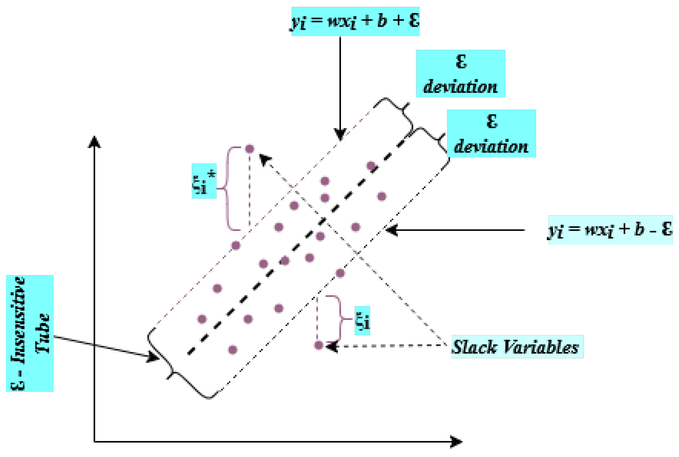
Support Vector Machine is a well-liked ML technique for classification and regression. SVM Regression also called SVR [45] is a commonly used technique for the prediction and curve fitting for linear as well as non-linear types of regression [46]. It is based on SVM in which support vectors are the points that are closer to the generated hyperplane that segregates the data points about the hyperplane as shown in Figure 1.
Support Vector Regression aims to identify a function that approximates the connection between the predictor X and the target feature Y on a given training dataset . The -insensitive tube loss function is introduced by SVR, which states that only those points are considered errors that are beyond the threshold point. Minimizing the cost function as shown in Eq. (1) is the main objective of SVR.
subject to:
Where w and b represent the weight vector and bias term respectively. The regularisation parameter C regulates the trade-off between reducing error and maximizing margin.
Slack variables , deal with hard cases to distinguish exactly. More detailed discussion on SVM and SVR can be found on [47].
Figure 1.
Support Vector Regression.
3.2. Random Forest
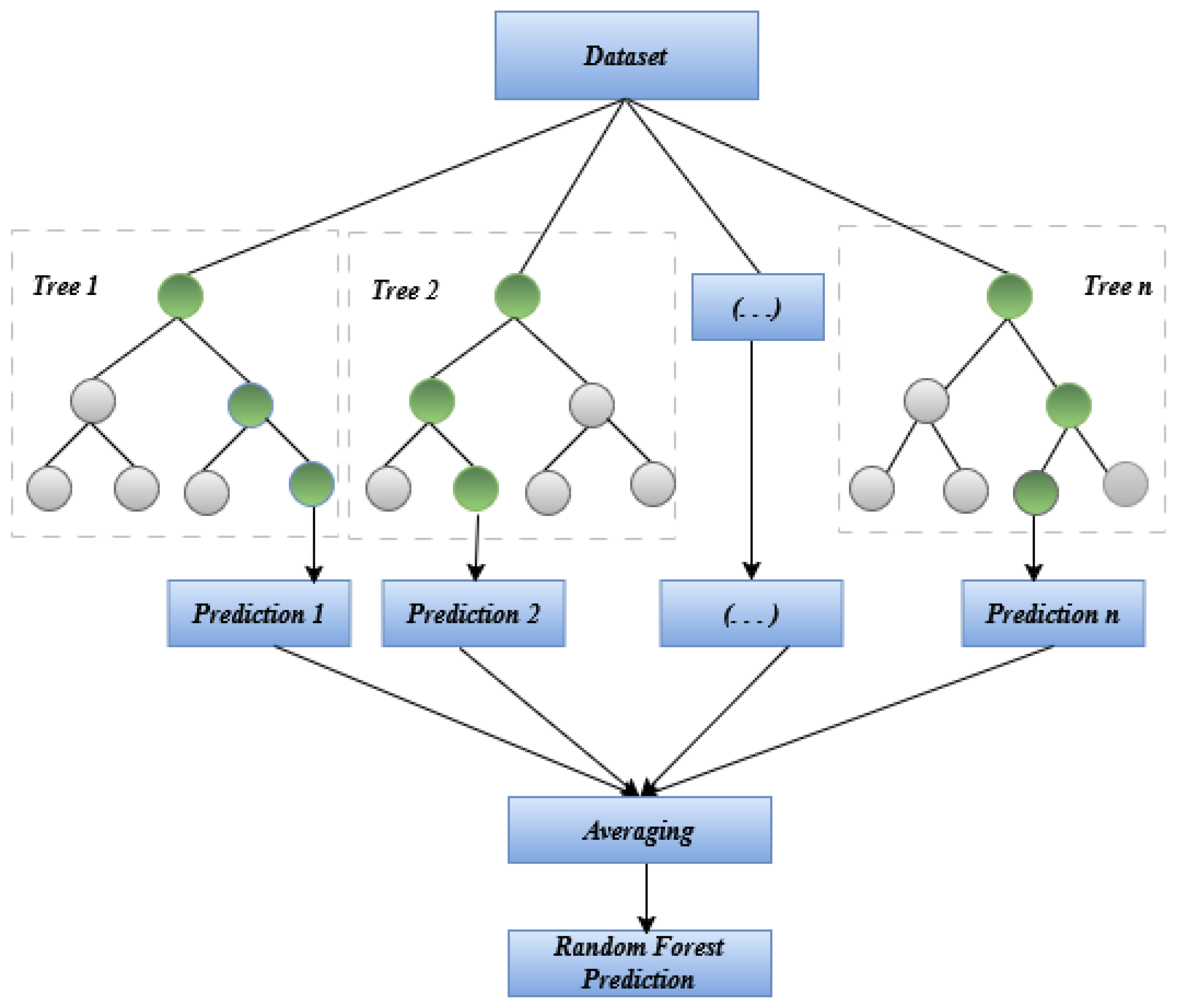
Several machine-learning applications can make use of decision trees. A tiny bit of noise in the data may cause the tree to grow in an entirely different way [48]. RF tries to overcome this problem using multiple decision trees and training them on different subsets of the features set at the cost of slightly increased bias i.e., all the trees in RF see only part of the entire training set [49]. Splitting of training sets into partitions is recursively done as shown in Figure 2. The choice of splitting at a particular node depends on some impurity measure like Shannon Entropy or Gini impurity for the classification problem [50]. Stock price prediction is a regression problem, so a measure is needed that shows how much the model prediction deviates from the actual value.
Some hyper-parameters of random forests need to be optimized for better performance and to control the model from overfitting. These are n_estimators, max_depth, max_features, min_samples_split etc.
Figure 2.
Workflow of Random Forest.
3.3. Extreme Gradient Boosting (XGBoost)
XGBoost, for short, stands for Improvement of Distributed Gradient Boost Decision Tree (GBDT). XGBoost is generally more precise than GBDT and boosts computational speed and performance [51]. In this, features are repeatedly split to add new trees. Adding new trees each time is learning a new function to fit the residual of the last prediction. When k number of trees are produced after training, each tree has a corresponding leaf node which represents a score. Finally, the recognition prediction value of the sample is calculated by adding the corresponding scores of each tree [52] as shown in Figure 3.
There are several benefits related to XGBoost that make it ideal for financial research. First and foremost, it is an effective tool for handling massive amounts of data without sacrificing efficiency, which is essential for working with time-series data that is a part of stock market analysis. Secondly, it offers valuable insights into feature significance, facilitating the identification of elements that have the greatest impact on fluctuations in stock prices [53]. Moreover, XGBoost supports parallel processing, which leverages several processor cores to accelerate the training process [54]. It also provides significant benefits for financial institutions, analysts, and investors in navigating the intricate world of finance.
3.4. Lasso Regression
The explosive growth of data in modern research and industry has led to an increasing need for efficient methods for feature selection and predictive modelling. Lasso regression is an essential tool in predictive modelling and offers a principled approach to handling high-dimensional data by introducing a penalty term to the ordinary least squares objective function [55]. This approach effectively performs automatic variable selection and reduces overfitting [56]. It has the ability to strike a balance between bias and variance, making it a popular choice across various fields, from biomedical research to finance, where identifying key predictive factors is crucial for effective decision-making. The objective function of Lasso Regression is shown below in Eq. (2).
Where is the observed value for the ith sample, is the value of the jth feature for the ith sample, is the intercept term, βj is the coefficient for the jth feature, p is the number of features, and is the regularization parameter that controls the strength of the penalty term. The key component in lasso regression is the penalty term . It penalizes the coefficients’ absolute values, causing some of them to decrease towards zero [57]. This favors the solutions in which large number of coefficients are exactly zero, because of this property lasso regression automatically selects a subset of features and shrinks the others towards zero.
3.5. Artificial Neural Network
An ANN is a network of mathematical equations that receives one or more inputs, processes these inputs using these equations, and produces one or multiple outputs. Generally, there are three layers present in every network- an input layer, a hidden layer, and an output layer. The input layer is responsible for data reception, feature representation and data transfer. The hidden layer performs intermediate computation and learning through backpropagation. The output layer is responsible for producing the results based on learned transformation. In neural network structure, the number of input and output layers is always one, but the hidden layers vary depending upon the complexity of the problem [47]. The hidden layer is regarded as the most critical layer because it serves as a distillation layer that transfers only the required information to the next layer making the network more efficient and speedy [58]. Figure 4 shows the general architecture neural network with the input layer, output layer, and multiple hidden layers. The precise estimation of weights is the key to obtaining a high-quality model, and this task can be achieved by using the concept of backpropagation.
3.6. EvoBagNet: Proposed Ensemble Bagging Learning Models with Evolutionary Algorithm
3.6.1. Ensemble Learning Models
Ensemble prediction models are powerful tools designed to significantly enhance the predictive performance of individual statistical learning techniques or model-fitting approaches. By leveraging the strengths of multiple models, ensemble methods aim to achieve superior accuracy and robustness in predictions, often outperforming single-model approaches [59]. The core principle of ensemble methods lies in their ability to combine multiple models—whether through linear or nonlinear aggregations—rather than depending solely on a single model fit. This approach enables ensembles to capture better the complexities, variabilities, and nonlinear patterns inherent in the dataset, reducing the risk of overfitting and improving generalization across diverse data scenarios.
Popular ensemble techniques [60] include Bagging, which reduces variance by training multiple models on bootstrapped datasets and averaging their predictions; Boosting, which sequentially improves weak models by focusing on hard-to-predict instances; and Stacking, which integrates predictions from multiple base models using a meta-model to optimize overall performance. These methods exemplify the versatility and effectiveness of ensemble approaches in addressing a wide range of predictive tasks.
3.6.2. Bagging Ensemble Models
The bagging ensemble model, often referred to by the more formal term bootstrap aggregating, serves a crucial role in enhancing the reliability and stability of estimation or classification methods that may otherwise exhibit erratic behaviour. Breiman [61] initially proposed bagging as a technique explicitly aimed at reducing variance for a designated foundational procedure, which could include various approaches such as decision trees or different methodologies designed for selecting variables and fitting within a linear modelling framework. This innovative technique has garnered significant interest over the years, and this heightened curiosity can likely be attributed to its straightforward implementation coupled with the widespread acceptance and application of the bootstrap method. At the moment when this groundbreaking concept was introduced to the community, only intuitive and informal arguments were put forth to explain the mechanisms behind why bagging would yield effective results. Subsequently, another research [62] revealed that bagging functions as a smoothing operation, which ultimately proves to be beneficial when the objective is to enhance the accuracy of predictive outcomes in both regression and classification trees. In particular, with regard to decision trees, the theoretical insights provided by [62] lend credence to Breiman’s original hypothesis that bagging serves as a technique for variance reduction, which simultaneously diminishes the mean squared error (MSE) associated with predictions. This principle similarly applies to subagging, or subsample aggregating, which is characterized as a more computationally efficient alternative to the traditional bagging approach. Nevertheless, it is important to note that when applied to other types of base procedures, even those deemed "complex," the advantageous effects of variance and MSE reduction attributed to bagging cannot be guaranteed with the same certainty.
In the context of regression or classification tasks, we often deal with pairs denoted as , where represents a d-dimensional predictor variable that exists within . In contrast, the response variable can either belong to the real numbers for regression tasks, denoted as , or take on discrete values for classification tasks, where belongs to the set , indicating that there are M distinct classes to categorize. The target function that we typically seek to estimate is represented by the expression in the case of regression or by the multivariate function in the context of classification problems, where our goal is to ascertain the relationship between the predictors and the response variables. The estimator of the function, which arises from applying a specified base procedure, is formulated accordingly.
The technical details of Bagging are as follows.
- The bootstrap group should be made randomly doing n times with substitution from the data .
- The bootstrapped estimator should be calculated by considering:
- Iterate previous levels Z times, which is optional depending on the various parameters such as sample size and complexity, yielding . The bagged estimator is .
In the theoretical framework, the quantity is associated with the scenario where ; however, in practical applications, the finite number Z significantly influences the precision of the Monte Carlo approximation, yet it should not be misconstrued as a parameter that requires tuning specifically for bagging methodologies.
There is a substantial body of empirical evidence that demonstrates bagging’s efficacy in enhancing the predictive performance of regression and classification trees, and this is now widely acknowledged within the statistical community. To illustrate the extent of the performance enhancement attributable to bagging, it references some of the findings from [61], which highlights that across seven distinct classification challenges, applying bagging to a classification tree yielded improvements over the performance of a solitary classification tree, particularly in terms of the cross-validated misclassification error rate, showcasing the method’s robustness. In both the regression and classification scenarios, the dimensions of the single decision tree, as well as the bootstrapped trees, were carefully selected through a process that involved optimizing for a tenfold cross-validated error, employing what is considered the conventional type of tree procedure that statisticians typically use. Moreover, while the reported enhancements in predictive accuracy are quite remarkable, it is essential to note that bagging a decision tree rarely performs worse in terms of predictive capability than utilizing a single tree alone. A straightforward equality illustrates the somewhat unconventional methodology that is employed when utilizing the bootstrap technique:
where stands for the bootstrap bias estimate associated with . Rather than adhering to the conventional bias correction that comes with a negative sign, bagging introduces a rather unexpected twist by incorporating the bootstrap bias estimate with a positive sign. Consequently, one might anticipate that bagging would produce a higher bias compared to , a notion that we will substantiate in some respects. However, in keeping with the traditional interplay between bias and variance as understood in nonparametric statistics, the overarching hope is to achieve a greater reduction in variance than the increase in bias, thus leading to an overall beneficial outcome concerning the mean squared error (MSE). Interestingly, this optimistic outlook tends to hold true for several base procedures that are employed. Indeed, The original algorithm [61] offered a heuristic description of bagging’s performance, asserting that the variance of the bagged estimator should be equal to or less than that of the original estimator , and in situations where the original estimator exhibits "instability," there can be a significant reduction in variance that further enhances the model’s reliability and accuracy.
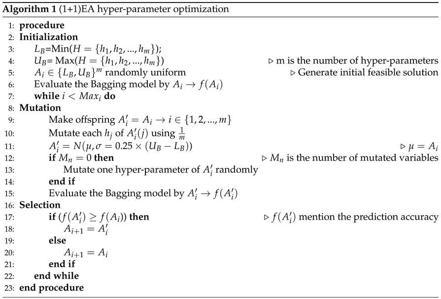
3.6.3. Single-Based Evolutionary Algorithm ()
In this research, we aim to improve the performance of the Bagging ensemble learning model by optimizing its hyper-parameters using 1+1 Evolutionary Algorithm (1+1EA), a straightforward yet highly effective single-solution evolutionary algorithm [63]. Empirical evidence suggests that simple evolutionary algorithms can often outperform more complex approaches, particularly in cases where the fitness function involves combinatorial optimization [64].
The 1+1EA operates by starting with an initial candidate solution (A) and generating a new solution () in each iteration through random modifications, achieved by flipping one or more variables of A with a mutation probability of . Unlike the standard version, where mutation follows a uniform distribution leading to unstructured and noisy local searches, we utilize a normally distributed mutation. This approach enables a gradual progression toward near-optimal solutions, although it may become computationally expensive for large-scale optimization problems.
The pseudo-code for the 1+1EA is provided in Algorithm 1. Here, and denote the upper and lower bounds of the variables, respectively, while m refers to the number of hyper-parameters. Additionally, to address scenarios where no variables are mutated during a single iteration, an alternative mutation strategy ensures at least one variable’s size is adjusted randomly to maintain progress in the optimization process.
 |
The proposed evolutionary ensemble model described in the previous section is visualized and can be seen in Figure 5.
3.7. Evaluation Metrics
After the deployment of ML models, Performance evaluation is the critical step to ensure continued effectiveness and accuracy. This study used four evaluation metrics to evaluate the performance of the proposed approaches: MAPE, R2, RMSE, and MAE.
MAPE is a percentage-based metric that measures the error in terms of percentage and gives interpretable thinking about the quality of prediction [65]. It is a scale-independent metric and is the most commonly used percentage metric that calculates average percentage error. MAPE is defined as shown in Eq. (5):
where represents the predicted value, represents the actual value and n represents the total number of records
R2 is also called the coefficient of determination, is a correlation-based metric that is mostly used with regression models to evaluate the goodness of linear fit [66]. It is calculated as in Eq. (6):
represents the predicted and actual values respectively, is the mean of actual variable and n is the amount of data collected.
Root Mean Square Error (RMSE) is a machine learning assessment metric that is particularly applied in regression tasks to compute the average magnitude of error between actual and predicted values. RMSE is a scale-dependent metric which means its scale is the same as the original data and provides errors in the same unit [67]. RMSE is calculated as in Eq. (7).
Another metric, Mean Absolute Error (MAE), is widely applied in statistics and ML for evaluating the performance of regression models [68]. It computes the average magnitude of errors between the actual price and the predicted price without taking into account their direction. It is computed as shown in Eq. (8).
4. Modeling Stock Market Analysis
This study proposes an adaptive bagging ensemble learning model for stock price prediction with exceptional and acceptable results as compared to the earlier strategies employed in the stock market. The proposed techniques use historical data to forecast the next day’s closing price of IT giant companies. Nine state-of-the-art machine-learning techniques have been deployed for stock market prediction. Different parameter configurations were tested during the experimentation to optimize ML approaches. In general, there are five main phases in the experimental setting: (i) Data analysis and preparation, (ii) model development and training, (iii) model optimization, (iv) deployment of optimized approaches on the test set, (v) the last step is result evaluation and comparative analysis as shown in Figure 5, and a detailed discussion of each step will be in subsequent sections.
4.1. Dataset
The first step in initiating the process of prediction is to collect the data. After a deep qualitative study to identify reliable sources for stock market data, the National Stock Exchange (NSE) provides up-to-date information related to the stocks. For experimentation, the dataset of Top IT companies has been collected from the same source as shown in Table 2 and is in Comma Separated Values (CSV) format. All the datasets exclude non-trading days such as weekends and holidays to offer a more accurate and trustworthy evaluation of market trends. Figure 6 illustrates the per year number of trading days included in the dataset. These selected companies are the key players in the NiftyIT index; each company has its capabilities, strengths, and contributions to the technology landscape. The daily information regarding the stock market is publicly available on the NSE website, which includes the following key attributes:
- Date represents the date on which the stock market information is reported.
- Series represents the security type that is being traded; it is EQ( equity).
- Open represents the price of the first trade of the security at the start of a trading day.
- High represents the highest price of the stock in a day.
- Low represents the lowest price of the stock in a day.
- Prev. Close the previous day’s closing price of the security.
- LTP (Last Traded Price) is the price at which the last trade for a security has occurred.
- Close is the price of the security at the closing of the trading session.
- VWAP (Volume Weighted Average Price) is the average price of the security weighted by volume.
- 52WH is the highest price of the security traded over the last 52 weeks.
- 52WL is the lowest price of the security traded over the last 52 weeks.
- Volume is the number of shares traded in a day.
- Value is the total value of all trades executed in a day.
- No. of Trades is the total number of trades executed in a day.

Table 2.
Description of Dataset.
| Stock | Date | Weightage in Nifty IT 4 | Source |
|---|---|---|---|
| Infosys | 01-Jan-2020 to 01-Jan-2024 (Total 1252 trading days) | 26.45% | NSE |
| TCS | 01-Jan-2019 to 01-Jan-2024 (Total 1252 trading days) | 23.26% | NSE |
| HCL | 01-Jan-2019 to 01-Jan-2024 (Total 1252 trading days) | 10.69% | NSE |
| Tech Mahindra | 01-Jan-2019 to 01-Jan-2024 (Total 1252 trading days) | 10.46% | NSE |
| Wipro | 01-Jan-2020 to 01-Jan-2024 (Total 1252 Trading Days) | 7.99% | NSE |
| LTIMindtree | 01-Jan-2019 to 01-Jan-2024 (Total 1252 trading days) | 5.41% | NSE |
| Coforge | 01-Jan-2019 to 01-Jan-2024 (Total 1252 trading days) | 5.18% | NSE |
| MphasiS | 01-Jan-2019 to 01-Jan-2024 (Total 1252 trading days) | 3.33% | NSE |
| L and T Technology Services | 01-Jan-2019 to 01-Jan-2024 (Total 1252 trading days) | 24.87% | NSE |
4.2. Data Preprocessing
Data preparation is an essential step to ensure that the raw data for machine learning models is in the right format for efficient training and analysis. In the current study, the data preparation step is sub-categorized into four distinct steps, and each step is discussed as follows:
4.2.1. Handle Missing Values
Due to some technical glitch, the collected dataset contains repeated entries and missing values. It’s essential to carefully preprocess the data and select the appropriate imputation strategies to address the missing data. There are different approaches to handling the missing data, in the current study Data Imputation approach has been applied. Data Imputation is a process in which missing values are filled with the values estimated based on available data. The stock market data is a time series data, so the mean imputation is not a suitable approach as done in [69]. In this work, the average of the previous and subsequent values is imputed to replace the missing value.
4.2.2. Data Normalization
In preprocessing, data normalization is the crucial step in statistical and ML modelling. It guarantees that all the features contribute equally, boosts the performance of the model, and accelerates the pace at which optimization techniques converge. There are various approaches for data normalization, but in this study, min-max scaling is applied and is done by using Eq. (9)
is the normalized feature value after applying min-max scaling, X is the actual feature value, and are the lowest and highest values of the feature in the dataset respectively.
4.2.3. Feature Selection
Machine Learning approaches perform better when features are carefully chosen. As observed from the literature survey, the stock market data is highly volatile and noisy, making the prediction very challenging; to improve the prediction accuracy, it is critical to comprehend the features and structure of the stock market data [70]. The following are the main causes of feature selection’s importance: firstly, feature reduction leads to fewer chances of model overfitting, and another reason is a better understanding of the features and their relationships with the target feature. Lastly, it reduces the computational time. There are different approaches to feature selection; in this study, the Recursive Feature Elimination (RFE) mechanism has been applied. This approach is widely used and is based on a greedy mechanism to choose the more relevant subset of features [71]. It is a wrapper method in which the score of each feature is calculated, and the feature with the lowest score is removed. This process is recursively repeated until the required feature set is obtained. The number of features to be chosen is given in advance to the algorithm. In this study, out of a total of 14 features, only nine relevant features were selected for further processing. It has been observed that the feature selection greatly affects the prediction’s performance. Figure 7 shown below depicts the working of RFE.
4.2.4. Data Partitioning
After preprocessing, different commonly used ratios were checked for data partitioning and for the training and testing of the machine learning models. These divisions help in the efficient assessment and validation of the model. In the current study, three data partitioning ratios, such as 70:30, 80:20, and 90:10, have been applied, and results achieved with all these are discussed later in the results section.
After completing the preprocessing, the next crucial step is implementing ML models that involve the selection of appropriate models, model training and tuning, and assessing model performance to ensure they provide reliable results.
5. Experimental Evaluation
This section presents the performance of ML approaches to understanding the effectiveness of the proposed study. It evaluates the efficacy of various models for the prediction of the stock market using different data-partitioning ratios. The change in the train test split ratio also impacts the reliability of the ML model [72]. The accuracy and stability of the model are enhanced by expanding the size of the training data. However, the drift is in a different direction when the latter has grown from 80% to 90%. Thus, the splitting ratio significantly affects the ML model’s predictive power. This study applied nine ML techniques: SVR, RF, XGB, LR, DT, LGBM, GBR, CAT B and ANN to predict closing prices based on different splitting ratios of input data. The dataset was split into 30/70, and 90/10 training and testing splitting ratios in addition to the most common ratio, the 80/20 ratio, and results achieved with all three splitting ratios were analyzed.
All approaches were implemented using Python and Keras, an open-source deep-learning library built on TensorFlow. The experiments were conducted in a computational environment featuring an Intel i7-8665U processor running at 2.11 GHz, 16 GB of RAM, and the Windows 10 Pro operating system. This setup ensured sufficient computational power and compatibility for training and evaluating the models.
In the first experiment, Support Vector Regression (SVR) was deployed on all nine datasets, with hyper-parameter tuning performed using grid search. The experiments were conducted using various train-test split ratios to analyze the model’s performance under different data distributions. The results are presented in Table 3. As shown, the highest prediction accuracy was achieved for the HCL dataset, with an accuracy of 95% and a Mean Absolute Error (MAE) of 15.22. Moreover, the results indicate that SVR is highly sensitive to the percentage of training data. Specifically, when the training data exceeds 70%, the model tends to overfit, leading to a reduction in test accuracy. This highlights the importance of selecting an optimal train-test split to balance training sufficiency and generalization capability for robust predictions.
Next, the performance of Random Forest (RF) was evaluated using various train-test split ratios across nine stock datasets. At first glance, RF demonstrated better average performance compared to SVR for all datasets, primarily due to its ability to capture complex and nonlinear relationships in the data effectively. With the exception of Wipro and HCL, which achieved accuracies of 89% and 86%, respectively, RF predicted the next day’s stock price with a high accuracy exceeding 90% for the remaining datasets. Additionally, it was observed that RF is less sensitive to the choice of train-test split ratios compared to SVM, making it more robust and reliable for stock price prediction tasks.
XGBoost is a widely used method for stock price forecasting, and its performance was evaluated across nine case studies, as shown in Table 5. The highest accuracy was achieved for the Coforge dataset at 94%, while the lowest accuracy was observed for the HCL dataset at 83%. This variation in accuracy can be attributed to differences in stock price volatility among companies. Stocks with more stable price movements tend to yield higher predictive accuracy, whereas higher volatility introduces greater uncertainty, making accurate forecasting more challenging.
Given its advantages in handling high-dimensional data, irrelevant or redundant features, and multi-collinearity, Lasso regression was employed in this study. Its ability to balance model simplicity with predictive performance makes it a robust tool for regression tasks. The results of Lasso regression for all case studies are summarized in Table 6. On average, Lasso regression delivered strong performance with an acceptable level of accuracy and MAE across most datasets. Notably, the highest accuracy was achieved for the HCL and LTI Mindtree datasets, both at 96%.
Another well-known machine learning model for stock price prediction is neural networks, renowned for their exceptional ability to extract nonlinear and complex patterns from data. This capability allows them to outperform traditional models, such as linear regression or decision trees, in capturing intricate relationships. Table 7 presents the prediction results of the NN model across nine case studies. Neural networks demonstrated effective performance for most datasets, achieving an accuracy exceeding 90%. Notably, the highest accuracy of 95% was observed for both the HCL and L&T Tech datasets.
5.1. Hyper-Parameter Tuning
Hyper-parameter tuning is the critical stage in the development of the ML model because hyper-parameters regulate the behaviour of the model during the training process. The selection of an optimal configuration that minimizes the error rate and maximizes accuracy can greatly improve the model performance on unseen data. This study implements hyper-parameter tuning to enhance model performance and also proved to be the more reliable and precise prediction of the next day’s closing price, indicating the effectiveness of our method in a volatile stock market environment. The hyper-parameters, range of values, and selected values are shown in Table 8, Table 9 and Table 10. In SVR, the trade-off between maximizing the margin and minimizing the training error is controlled by the regularization parameter C. If the value of C is small, that allows a wider margin, but it may lead to huge training errors, epsilon is the tolerance margin around the predicted value. It is the point at which training mistakes do not result in a penalty. It regulates the tube’s diameter, beyond which faults are deemed negligible, () is used to characterize the influence of a single training sample, with high values indicating ‘near’ and low values indicating ‘far’. It establishes how adaptable the decision limit is. In Random Forest, three hyper-parameters have been optimized: n_estimators control the number of decision trees that will be running in the forest, max_depth controls the maximum depth of each decision tree, and min_samples_split represents the minimum number of samples required to split an internal node. In the case of the XGBoost approach, here also three hyper-parameters are optimized, n_estimators and max_depth are already defined, and the third is learning_rate. The learning rate determines the step size at every boosting iteration. By taking fewer steps, lower learning rate values strengthen the model; nevertheless, it can take more boosting rounds for it to converge. In Lasso Regression, only one hyper-parameter is optimized; that is, , alpha regulates the strength of the penalty term in the lasso objective function. It keeps the model simple and fits the training set well. Higher alpha values mean more regularization, which leads to more coefficients in the direction of zero.
Hyper-parameter tuning is highly beneficial for ANN because of its numerous parameters. Six hyper-parameters are optimized, including epochs, learning rate (LR), hidden layers, activation function, dropout, and shape. The hyper-parameter epoch represents how often the training data is passed to the neural network, and in the proposed study, three values of epochs are supplied. An important hyper-parameter lr is used to control the model’s step size during optimisation. Choosing the appropriate value of lr is very important because a higher value may overshoot the optimal result, and using a lower value may take a longer time. Another hyper-parameter is hidden layers, which represents the number of layers between input and output layers. Activation function Relu has been used because it is computationally efficient and involves simple thresholding. Sometimes the model leads to overfitting, dropout is used to control the overfitting. The range of value is passed to the model for selecting the optimal one; the last hyper-parameter is the shape of the neural network, which represents the structural design of neurons and can be either brick or funnel. This hyper-parameter also impacts the learning capability of the network. In ANN, a validation set has been used to adjust the hyper-parameters and to avoid overfitting. This also helps to make sure the model generalizes effectively to new data. In this, the ‘Scan’ function of the Talos library has been used to traverse both training and validation sets for the adjustment of hyper-parameters. This function analyzes all the permutations and combinations of hyper-parameter values that are supplied, as shown in Table 10. Another object in the same library is ‘Analyze’, which is used to carry out all the outcomes of the tuning activity. To obtain the optimal configuration of the model, Talos.best_model(metric: low MAPE) is used, and this model is the final optimized model that is finally applied to the test set.
Table 8.
Hyper-parameters and their selected values of SVR and Random Forest.
| SVR | Random Forest | ||||
|---|---|---|---|---|---|
| Hyperparameter | Values | Selected Value | Hyperparameter | Values | Selected Value |
| C | [0.1, 1, 10, 100] | 100 | n_estimators | [100, 200, 300, 400] | 100 |
| gamma | [0.1, 0.01, 0.001] | 0.01 | max_depth | [3, 4, 5, 6, 7] | 5 |
| epsilon | [0.1, 0.01, 0.001] | 0.1 | min_samples_split | [2, 3, 4, 5, 10] | 3 |
Table 9.
Hyper-parameters and their selected values of XGBoost and Lasso Regression.
| XGBoost | Lasso Regression | ||||
|---|---|---|---|---|---|
| Hyperparameter | Values | Selected Value | Hyperparameter | Values | Selected Value |
| n_estimators | [200, 300, 400] | 400 | alpha | [0.001, 0.01, 0.1, 1, 10] | 1 |
| max_depth | [3, 5, 7] | 7 | |||
| Learning_rate | [0.02, 0.03, 0.05, 0.1, 0.2] | 0.1 | |||
Table 10.
Hyper-parameters and their best-selected values of Artificial Neural Network.
| Hyper-parameter | Values | Selected Value | Hyper-parameter | Values | Selected Value |
| epochs | [300, 400, 500] | 500 | dropout | (0 to 0.5) 3 levels | 0.0 |
| lr | (0.01 to 0.05) 3 levels | 0.036 | Activation function | [relu] | relu |
| Hidden layers | [1, 2, 3] | 2 | shape | [brick, funnel] | funnel |
As the complexity and volume of financial data continuously increase, effective visualization approaches are becoming more and more necessary for interpreting and understanding predictive models in the domain of the equity market. This research investigates the utility of interactive line plots as a visualization aid for displaying the real price and the forecasted price. While using the interactive nature of line plots, users may examine model performance by zooming in/Out, hovering over data points, and pinpointing possible areas for improvement by panning between periods. In the proposed study, only the best results achieved are shown using the interactive line plot. The proposed training set is used for training the model, and the models achieved by training are used to predict the test set data and the real value is compared with the predicted value as shown in Figure 8 (a to O). In this figure, (a), (b), and (c) represent the actual stock price and predicted stock price using SVR applied on Infosys, TCS, and Wipro, figures (d), (e), and (f) show the prediction of Random forest applied on same datasets. Similarly, the remaining figures show the prediction of XGB, Lasso regression, and optimized ANN. As per the actual values and predicted values achieved using each method, the error calculation of each technique is done, and finally, a comparison of the results is made.
5.2. Comparative Analysis
This section compares the proposed approaches based on the evaluation metrics. As already known, when the MAPE value is close to zero, and R2 close to 1, the model performs well. One example of individual ML models’ performance for three datasets can be seen in Figure 9, and it is interpreted from the chart that ANN with deep hyper-parameter tuning showed better results as compared to the others. The other two evaluation metrics, RMSE and MAE, are scale-dependent, i.e. if the datasets are of different scales, then using RMSE and MAE this way may not provide a fair model comparison. In our study, three datasets are also of different scales, which is the main reason for comparing the model results (based on RMSE and MAE) differently, as shown in Figure 10.
To provide a more accurate comparison among the six proposed bagging models, we present Table 11. The table extensively evaluates the performance of these models on the Coforge time series data using six distinct metrics. As illustrated in Table 11, all proposed models achieved high prediction accuracy, exceeding 97%. Notably, the best-performing model was Bag-DT, which attained an accuracy of 98.5%, demonstrating its superior capability in forecasting stock prices.
For the L&T Tech dataset, all proposed ensemble models demonstrated exceptional performance, achieving a prediction accuracy above 98% (), as shown in Table 12. Among these, Bag-LGBM and Bag-RF outperformed the other models in terms of Mean Absolute Error (MAE) and Root Mean Square Error (RMSE). A key observation from these results is the robustness of the proposed models, as evidenced by their consistent performance across K-fold cross-validation. Furthermore, the low variability in predictions, indicated by a small standard deviation (STD), underscores the model’s ability to reliably capture learned patterns without significant deviations, enhancing its dependability for accurate forecasting.
Figure 11 presents the statistical performance of the bagging models across nine datasets using the R2 metric. Notably, the Bag-GRB model demonstrated superior performance compared to other bagging ensemble models in most case studies. It also exhibited lower variance in performance across multiple training and testing splits, indicating higher stability and robustness. Among the datasets, the HCL dataset posed the greatest challenge due to the high dynamics of its stock price. Despite this, the prediction accuracy of all bagging models remained significant and reliable across all nine case studies, showcasing their effectiveness in handling diverse datasets.
Figure 12 provides a comprehensive comparison of the six proposed bagging models across nine datasets based on the Mean Absolute Error (MAE). Among these, Bag-GBR consistently achieved the lowest learning error in most case studies, demonstrating its superior predictive accuracy. However, Bag-LGBM exhibited notable performance specifically for the Tech Mahindra and TCS datasets, outperforming other models in these cases. These findings highlight the efficiency and reliability of the proposed models in accurately forecasting stock prices in advance.
6. Conclusions
The expanding engagement in stock markets, driven by rapid economic advancements, has intensified the need for accurate stock price prediction to enhance investment outcomes and reduce risks. Traditional statistical and machine learning approaches often fall short due to the unpredictable nature of stock prices, which are characterized by high volatility and dynamic fluctuations. To tackle these challenges, this study presents EvoBagNet, a novel evolutionary bagging ensemble framework designed to deliver robust and reliable stock price predictions.
EvoBagNet leverages a diverse array of nine advanced machine learning techniques, including tree-based algorithms, neural networks, and ensemble approaches, and applies them to datasets from nine leading IT sector companies. Through extensive experimentation with various train-test splits, EvoBagNet demonstrated outstanding performance, which was evaluated using six different metrics. The model achieved exceptional prediction accuracy, including , , , , , , , , and for Tech Mahindra, Mindtree, Infosys, Wipro, TCS, Mphasis, L&T Tech, HCL, and Coforge, respectively. These results highlight EvoBagNet’s ability to deliver accurate predictions consistently, even for volatile datasets such as HCL.
By addressing the shortcomings of traditional approaches, EvoBagNet stands out as a reliable tool for stock price prediction, offering practical value for investment strategies and risk management. Its demonstrated accuracy and robustness across diverse scenarios establish it as a promising model for real-world applications in dynamic and volatile financial markets. This study underscores the potential of EvoBagNet to drive innovation in financial forecasting and enhance decision-making in complex economic landscapes.
In the future, several approaches can increase the reach and usefulness of this study for stock market prediction. First, using a wider variety of data as inputs to the model- such as macroeconomic variables, news sentiment analysis, or economic indicators could offer a more comprehensive understanding of the effects on stock prices, which might improve the algorithms’ prediction accuracy. Second, more advanced sequential deep learning approaches like Bi-LSTM, Stack-LSTM, CNN-LSTM, etc., can be deployed for better prediction results. Third, the suggested model’s generalizability will be tested by cross-industry validations using datasets from different sectors, guaranteeing its application across different economic scenarios. Lastly, real-time prediction might be investigated to evaluate the models’ practical applicability and efficiency in live market conditions.
Author Contributions
Conceptualization, U.B., K.S., V.M., and A.M.U.D.K.; methodology, U.B., K.S., V.M., A.M.U.D.K., and M.N.; software, U.B., K.S., V.M., and A.M.U.D.K.; validation, U.B., V.M., and A.M.U.D.K.; formal analysis, U.B., V.M., and A.M.U.D.K.; investigation, U.B., K.S., V.M., A.M.U.D.K., and M.N.; resources, U.B., V.M., and A.M.U.D.K.; data curation, U.B., K.S., V.M., and A.M.U.D.K.; writing—original draft preparation, U.B., V.M., A.M.U.D.K., and M.N.; writing—review and editing, U.B., K.S., V.M., A.M.U.D.K., and M.N.; visualization, U.B., A.M.U.D.K., and M.N.; supervision, K.S., V.M., and A.M.U.D.K.; project administration, K.S., V.M., and A.M.U.D.K.; funding acquisition, U.B., K.S., and V.M. All authors have read and agreed to the published version of the manuscript.
Funding
This work was supported by ASPIRE Award for Research Excellence (AARE-2020). (ASPIRE award number AARE20-100 grant #21T055).
Informed Consent Statement
Not applicable
Data Availability Statement
Data will be available on request to akibkhanday@uaeu.ac.ae, umar.bashir@jammuuniversity.ac.in and code can be found at https://github.com/Akibkhanday/, https://github.com/UmarBashir131/.
Conflicts of Interest
The authors declare no conflicts of interest.
References
- Jafar, S.H.; Akhtar, S.; El-Chaarani, H.; Khan, P.A.; Binsaddig, R. Forecasting of NIFTY 50 index price by using backward elimination with an LSTM model. Journal of Risk and Financial Management 2023, 16, 423. [Google Scholar] [CrossRef]
- Hasan, F.; Al-Okaily, M.; Choudhury, T.; Kayani, U. A comparative analysis between FinTech and traditional stock markets: using Russia and Ukraine war data. Electronic Commerce Research 2024, 24, 629–654. [Google Scholar] [CrossRef]
- Jiang, W. Applications of deep learning in stock market prediction: recent progress. Expert Systems with Applications 2021, 184, 115537. [Google Scholar] [CrossRef]
- Hoque, H.; Doukas, J. Endogenous market choice, listing regulations, and IPO spread: Evidence from the London Stock Exchange. International Journal of Finance & Economics 2024, 29, 2360–2380. [Google Scholar] [CrossRef]
- Yuan, X.; Yuan, J.; Jiang, T.; Ain, Q.U. Integrated long-term stock selection models based on feature selection and machine learning algorithms for China stock market. IEEE Access 2020, 8, 22672–22685. [Google Scholar] [CrossRef]
- Khan, W.; Malik, U.; Ghazanfar, M.A.; Azam, M.A.; Alyoubi, K.H.; Alfakeeh, A.S. Predicting stock market trends using machine learning algorithms via public sentiment and political situation analysis. Soft Computing 2020, 24, 11019–11043. [Google Scholar] [CrossRef]
- Yañez, C.; Kristjanpoller, W.; Minutolo, M.C. Stock market index prediction using transformer neural network models and frequency decomposition. Neural Computing and Applications 2024, 1–21. [Google Scholar] [CrossRef]
- Idrees, S.M.; Alam, M.A.; Agarwal, P. A prediction approach for stock market volatility based on time series data. IEEE Access 2019, 7, 17287–17298. [Google Scholar] [CrossRef]
- Ma, Y.; Mao, R.; Lin, Q.; Wu, P.; Cambria, E. Multi-source aggregated classification for stock price movement prediction. Information Fusion 2023, 91, 515–528. [Google Scholar] [CrossRef]
- Xia, H.; Weng, J.; Boubaker, S.; Zhang, Z.; Jasimuddin, S.M. Cross-influence of information and risk effects on the IPO market: exploring risk disclosure with a machine learning approach. Annals of Operations Research 2024, 334, 761–797. [Google Scholar] [CrossRef]
- Al-Khasawneh, M.A.; Raza, A.; Khan, S.U.R.; Khan, Z. Stock Market Trend Prediction Using Deep Learning Approach. Computational Economics 2024, 1–32. [Google Scholar] [CrossRef]
- Ajiga, D.I.; Adeleye, R.A.; Tubokirifuruar, T.S.; Bello, B.G.; Ndubuisi, N.L.; Asuzu, O.F.; Owolabi, O.R. Machine learning for stock market forecasting: a review of models and accuracy. Finance & Accounting Research Journal 2024, 6, 112–124. [Google Scholar] [CrossRef]
- Sheth, D.; Shah, M. Predicting stock market using machine learning: best and accurate way to know future stock prices. International Journal of System Assurance Engineering and Management 2023, 14, 1–18. [Google Scholar] [CrossRef]
- Almaafi, A.; Bajaba, S.; Alnori, F. Stock price prediction using ARIMA versus XGBoost models: the case of the largest telecommunication company in the Middle East. International Journal of Information Technology 2023, 15, 1813–1818. [Google Scholar] [CrossRef]
- Parmar, A.; Katariya, R.; Patel, V. A review on random forest: An ensemble classifier. In Proceedings of the International Conference on Intelligent Data Communication Technologies and Internet of Things (ICICI) 2018; Springer, 2019; pp. 758–763. [Google Scholar] [CrossRef]
- Bentéjac, C.; Csörgo, A.; Martínez-Muñoz, G. A comparative analysis of gradient boosting algorithms. Artificial Intelligence Review 2021, 54, 1937–1967. [Google Scholar] [CrossRef]
- Natekin, A.; Knoll, A. Gradient boosting machines, a tutorial. Frontiers in Neurorobotics 2013, 7, 21. [Google Scholar] [CrossRef] [PubMed]
- Costa, V.G.; Pedreira, C.E. Recent advances in decision trees: An updated survey. Artificial Intelligence Review 2023, 56, 4765–4800. [Google Scholar] [CrossRef]
- Ke, G.; Meng, Q.; Finley, T.; Wang, T.; Chen, W.; Ma, W.; Ye, Q.; Liu, T.Y. Lightgbm: A highly efficient gradient boosting decision tree. Advances in Neural Information Processing Systems 2017, 30. [Google Scholar]
- Bhuriya, D.; Kaushal, G.; Sharma, A.; Singh, U. Stock market predication using a linear regression. In Proceedings of the 2017 International Conference of Electronics, Communication and Aerospace Technology (ICECA); IEEE, 2017; Vol. 2, pp. 510–513. [Google Scholar] [CrossRef]
- Dash, R.K.; Nguyen, T.N.; Cengiz, K.; Sharma, A. Fine-tuned support vector regression model for stock predictions. Neural Computing and Applications 2023, 35, 23295–23309. [Google Scholar] [CrossRef]
- Bansal, M.; Goyal, A.; Choudhary, A. Stock market prediction with high accuracy using machine learning techniques. Procedia Computer Science 2022, 215, 247–265. [Google Scholar] [CrossRef]
- Singh, G. Machine learning models in stock market prediction. arXiv 2022, arXiv:2202.09359. [Google Scholar] [CrossRef]
- Jain, S.; Kain, M. Prediction for Stock Marketing Using Machine Learning. Int. J. Recent Innov. Trends Comput. Commun. 131–135.
- Hemanth, D.; et al. Stock market prediction using machine learning techniques. Advances in Parallel Computing Technologies and Applications 2021, 40, 331. [Google Scholar] [CrossRef]
- Zhang, D.; Lou, S. The application research of neural network and BP algorithm in stock price pattern classification and prediction. Future Generation Computer Systems 2021, 115, 872–879. [Google Scholar] [CrossRef]
- Vijh, M.; Chandola, D.; Tikkiwal, V.A.; Kumar, A. Stock closing price prediction using machine learning techniques. Procedia Computer Science 2020, 167, 599–606. [Google Scholar] [CrossRef]
- Mustaffa, Z.; Sulaiman, M.H. Stock price predictive analysis: An application of hybrid barnacles mating optimizer with artificial neural network. International Journal of Cognitive Computing in Engineering 2023, 4, 109–117. [Google Scholar] [CrossRef]
- Zhong, X.; Enke, D. Predicting the daily return direction of the stock market using hybrid machine learning algorithms. Financial Innovation 2019, 5, 1–20. [Google Scholar] [CrossRef]
- Hao, Y.; Gao, Q. Predicting the trend of stock market index using the hybrid neural network based on multiple time scale feature learning. Applied Sciences 2020, 10, 3961. [Google Scholar] [CrossRef]
- Khan, W.; Ghazanfar, M.A.; Azam, M.A.; Karami, A.; Alyoubi, K.H.; Alfakeeh, A.S. Stock market prediction using machine learning classifiers and social media, news. Journal of Ambient Intelligence and Humanized Computing 2022, 1–24. [Google Scholar] [CrossRef]
- Chen, W.; Zhang, H.; Mehlawat, M.K.; Jia, L. Mean–variance portfolio optimization using machine learning-based stock price prediction. Applied Soft Computing 2021, 100, 106943. [Google Scholar] [CrossRef]
- Sharma, D.; Sarangi, P.K.; Sahoo, A.K.; et al. Analyzing the Effectiveness of Machine Learning Models in Nifty50 Next Day Prediction: A Comparative Analysis. In Proceedings of the 2023 3rd International Conference on Advance Computing and Innovative Technologies in Engineering (ICACITE); IEEE, 2023; pp. 245–250. [Google Scholar] [CrossRef]
- Ballings, M.; Van den Poel, D.; Hespeels, N.; Gryp, R. Evaluating multiple classifiers for stock price direction prediction. Expert Systems with Applications 2015, 42, 7046–7056. [Google Scholar] [CrossRef]
- Basak, S.; Kar, S.; Saha, S.; Khaidem, L.; Dey, S.R. Predicting the direction of stock market prices using tree-based classifiers. The North American Journal of Economics and Finance 2019, 47, 552–567. [Google Scholar] [CrossRef]
- Yetis, Y.; Kaplan, H.; Jamshidi, M. Stock market prediction by using artificial neural network. In Proceedings of the 2014 World Automation Congress (WAC); IEEE, 2014; pp. 718–722. [Google Scholar] [CrossRef]
- Shen, J.; Shafiq, M.O. Short-term stock market price trend prediction using a comprehensive deep learning system. Journal of Big Data 2020, 7, 1–33. [Google Scholar] [CrossRef] [PubMed]
- Senol, D.; Ozturan, M. Stock price direction prediction using artificial neural network approach: The case of Turkey. Journal of Artificial Intelligence 2009. [Google Scholar]
- Billah, M.M.; Sultana, A.; Bhuiyan, F.; Kaosar, M.G. Stock price prediction: comparison of different moving average techniques using deep learning model. Neural Computing and Applications 2024, 36, 5861–5871. [Google Scholar] [CrossRef]
- Nabipour, M.; Nayyeri, P.; Jabani, H.; Shahab, S.; Mosavi, A. Predicting stock market trends using machine learning and deep learning algorithms via continuous and binary data; a comparative analysis. IEEE Access 2020, 8, 150199–150212. [Google Scholar] [CrossRef]
- Kamalov, F. Forecasting significant stock price changes using neural networks. Neural Computing and Applications 2020, 32, 17655–17667. [Google Scholar] [CrossRef]
- Bathla, G.; Rani, R.; Aggarwal, H. Stocks of year 2020: prediction of high variations in stock prices using LSTM. Multimedia Tools and Applications 2023, 82, 9727–9743. [Google Scholar] [CrossRef]
- Sivadasan, E.; Mohana Sundaram, N.; Santhosh, R. Stock market forecasting using deep learning with long short-term memory and gated recurrent unit. Soft Computing 2024, 28, 3267–3282. [Google Scholar] [CrossRef]
- Elminaam, A.; Salama, D.; El-Tanany, A.M.M.; El Fattah, M.A.; Salam, M.A. StockBiLSTM: Utilizing an Efficient Deep Learning Approach for Forecasting Stock Market Time Series Data. International Journal of Advanced Computer Science & Applications 2024, 15. [Google Scholar] [CrossRef]
- Jin, S. A Comparative Analysis of Traditional and Machine Learning Methods in Forecasting the Stock Markets of China and the US. International Journal of Advanced Computer Science & Applications 2024, 15. [Google Scholar] [CrossRef]
- Parbat, D.; Chakraborty, M. A python based support vector regression model for prediction of COVID19 cases in India. Chaos, Solitons & Fractals 2020, 138, 109942. [Google Scholar] [CrossRef]
- Chhajer, P.; Shah, M.; Kshirsagar, A. The applications of artificial neural networks, support vector machines, and long–short term memory for stock market prediction. Decision Analytics Journal 2022, 2, 100015. [Google Scholar] [CrossRef]
- Elsayed, N.; Abd Elaleem, S.; Marie, M. Improving Prediction Accuracy using Random Forest Algorithm. International Journal of Advanced Computer Science & Applications 2024, 15. [Google Scholar] [CrossRef]
- Yin, L.; Li, B.; Li, P.; Zhang, R. Research on stock trend prediction method based on optimized random forest. CAAI Transactions on Intelligence Technology 2023, 8, 274–284. [Google Scholar] [CrossRef]
- Polamuri, S.R.; Srinivas, K.; Mohan, A.K. Stock market prices prediction using random forest and extra tree regression. Int. J. Recent Technol. Eng 2019, 8, 1224–1228. [Google Scholar] [CrossRef]
- Sharma, P.; Jain, M.K. Stock Market Trends Analysis using Extreme Gradient Boosting (XGBoost). In Proceedings of the 2023 International Conference on Computing, Communication, and Intelligent Systems (ICCCIS); IEEE, 2023; pp. 317–322. [Google Scholar] [CrossRef]
- Chen, T.; Guestrin, C. Xgboost: A scalable tree boosting system. In Proceedings of the 22nd ACM SIGKDD International Conference on Knowledge Discovery and Data Mining; 2016; pp. 785–794. [Google Scholar] [CrossRef]
- Saetia, K.; Yokrattanasak, J. Stock movement prediction using machine learning based on technical indicators and Google trend searches in Thailand. International Journal of Financial Studies 2022, 11, 5. [Google Scholar] [CrossRef]
- Dezhkam, A.; Manzuri, M.T. Forecasting stock market for an efficient portfolio by combining XGBoost and Hilbert–Huang transform. Engineering Applications of Artificial Intelligence 2023, 118, 105626. [Google Scholar] [CrossRef]
- Li, J.; Chen, W. Forecasting macroeconomic time series: LASSO-based approaches and their forecast combinations with dynamic factor models. International Journal of Forecasting 2014, 30, 996–1015. [Google Scholar] [CrossRef]
- Rastogi, A.; Qais, A.; Saxena, A.; Sinha, D. Stock market prediction with lasso regression using technical analysis and time lag. In Proceedings of the 2021 6th International Conference for Convergence in Technology (I2CT); IEEE, 2021; pp. 1–5. [Google Scholar] [CrossRef]
- Lee, J.H.; Shi, Z.; Gao, Z. On LASSO for predictive regression. Journal of Econometrics 2022, 229, 322–349. [Google Scholar] [CrossRef]
- Thakkar, A.; Chaudhari, K. CREST: cross-reference to exchange-based stock trend prediction using long short-term memory. Procedia Computer Science 2020, 167, 616–625. [Google Scholar] [CrossRef]
- Bühlmann, P. Bagging, boosting and ensemble methods. In Handbook of Computational Statistics: Concepts and Methods; 2012; pp. 985–1022. [Google Scholar] [CrossRef]
- Khan, A.A.; Chaudhari, O.; Chandra, R. A review of ensemble learning and data augmentation models for class imbalanced problems: combination, implementation and evaluation. Expert Systems with Applications 2024, 244, 122778. [Google Scholar] [CrossRef]
- Breiman, L. Bagging predictors. Machine Learning 1996, 24, 123–140. [Google Scholar] [CrossRef]
- Bühlmann, P.; Yu, B. Boosting with the L 2 loss: regression and classification. Journal of the American Statistical Association 2003, 98, 324–339. [Google Scholar] [CrossRef]
- Neshat, M. The application of nature-inspired metaheuristic methods for optimising renewable energy problems and the design of water distribution networks. PhD thesis, 2020. [Google Scholar]
- Neumann, F.; Wegener, I. Randomized local search, evolutionary algorithms, and the minimum spanning tree problem. Theoretical Computer Science 2007, 378, 32–40. [Google Scholar] [CrossRef]
- Flores, B.F. A Pragmatic View of Accuracy Measurement in Forecasting. OMEGA Int. J. Manag. Sci. 1986, 14, 93–98. [Google Scholar] [CrossRef]
- Kvålseth, T.O. Cautionary note about R 2. The American Statistician 1985, 39, 279–285. [Google Scholar] [CrossRef]
- Maçaira, P.M.; Cyrino Oliveira, F.L. Another look at SSA. Boot forecast accuracy. International Journal of Energy and Statistics 2016, 4, 1650008. [Google Scholar] [CrossRef]
- Cui, C.; Wang, P.; Li, Y.; Zhang, Y. McVCsB: A new hybrid deep learning network for stock index prediction. Expert Systems with Applications 2023, 120902. [Google Scholar] [CrossRef]
- Bhattacharjee, I.; Bhattacharja, P. Stock price prediction: a comparative study between traditional statistical approach and machine learning approach. In Proceedings of the 2019 4th International Conference on Electrical Information and Communication Technology (EICT); IEEE, 2019; pp. 1–6. [Google Scholar] [CrossRef]
- Kara, Y.; Boyacioglu, M.A.; Baykan, Ö.K. Predicting direction of stock price index movement using artificial neural networks and support vector machines: The sample of the Istanbul Stock Exchange. Expert Systems with Applications 2011, 38, 5311–5319. [Google Scholar] [CrossRef]
- Di Persio, L.; Honchar, O.; et al. Artificial neural networks architectures for stock price prediction: Comparisons and applications. International Journal of Circuits, Systems and Signal Processing 2016, 10, 403–413. [Google Scholar]
- Kulkarni, S. Impact of Various Data Splitting Ratios on the Performance of Machine Learning Models in the Classification of Lung Cancer. In Proceedings of the Proceedings of the Second International Conference on Emerging Trends in Engineering (ICETE 2023); Springer Nature, 2023; Vol. 223, p. 96. [Google Scholar]
| 1 | RSI: Relative strength index, SO: Stochastic oscillator, W%R: Williams percentage range, MACD: Moving average convergence divergence, PROC: Price rate of change, OBV: On balance volume |
| 2 | Istanbul Stock Exchange |
| 3 | Tehran Stock Exchange |
| 4 | As per NSE Indexogram dated October 31, 2024 |
Figure 3.
Workflow of XGB.
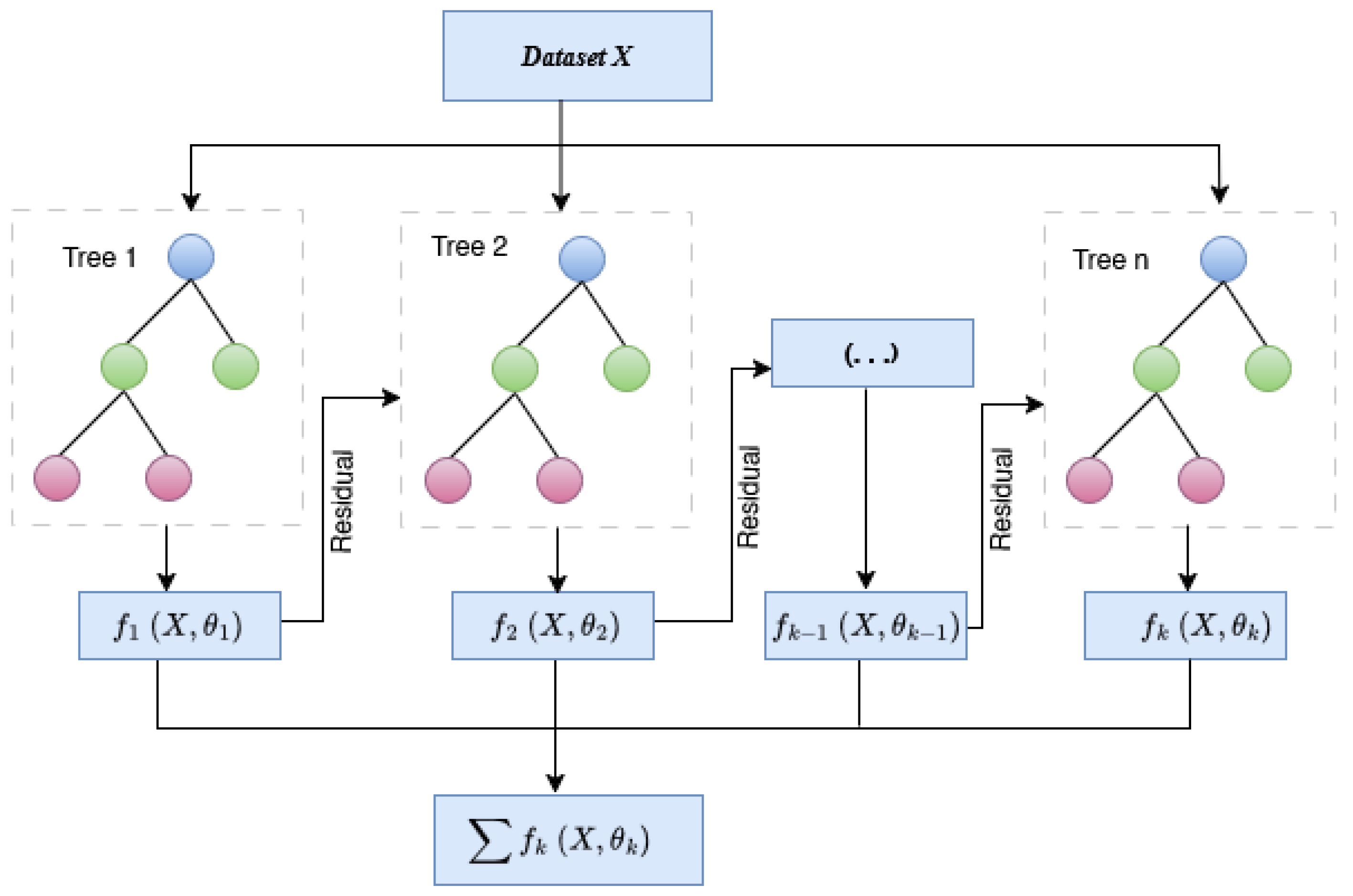
Figure 4.
Architecture of ANN.
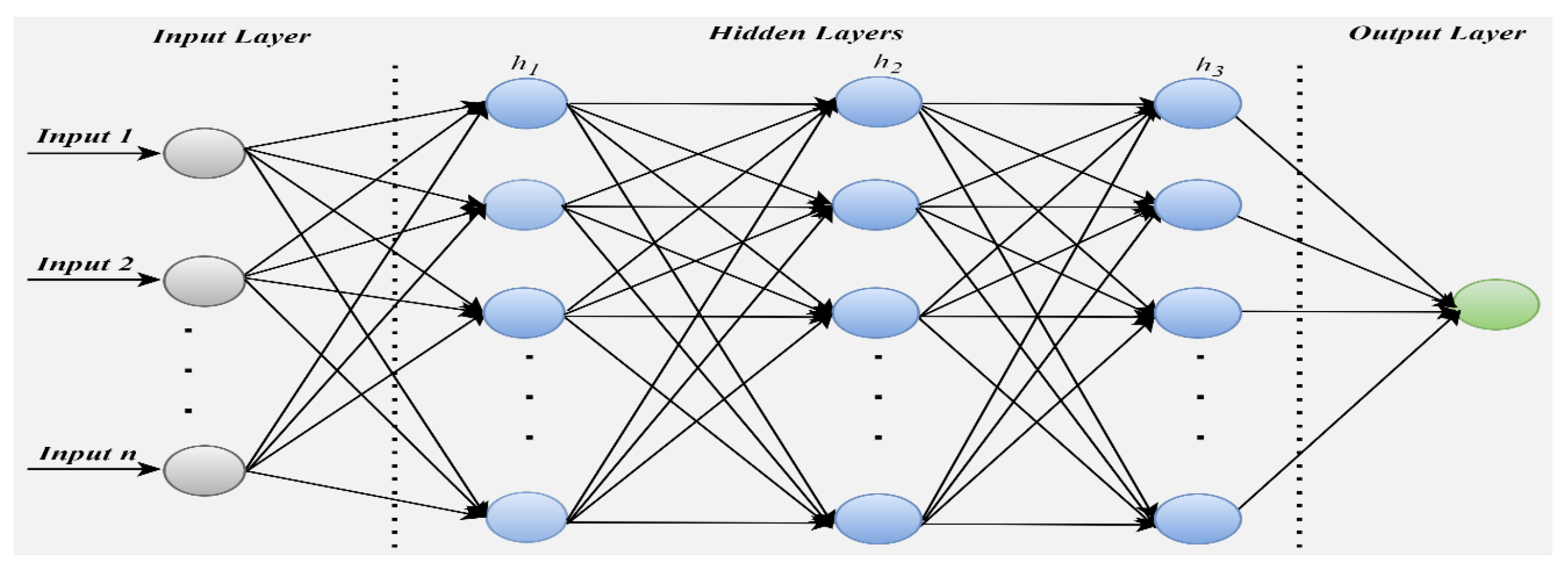
Figure 5.
The proposed EvoBagNet framework in predicting NSE time series data.
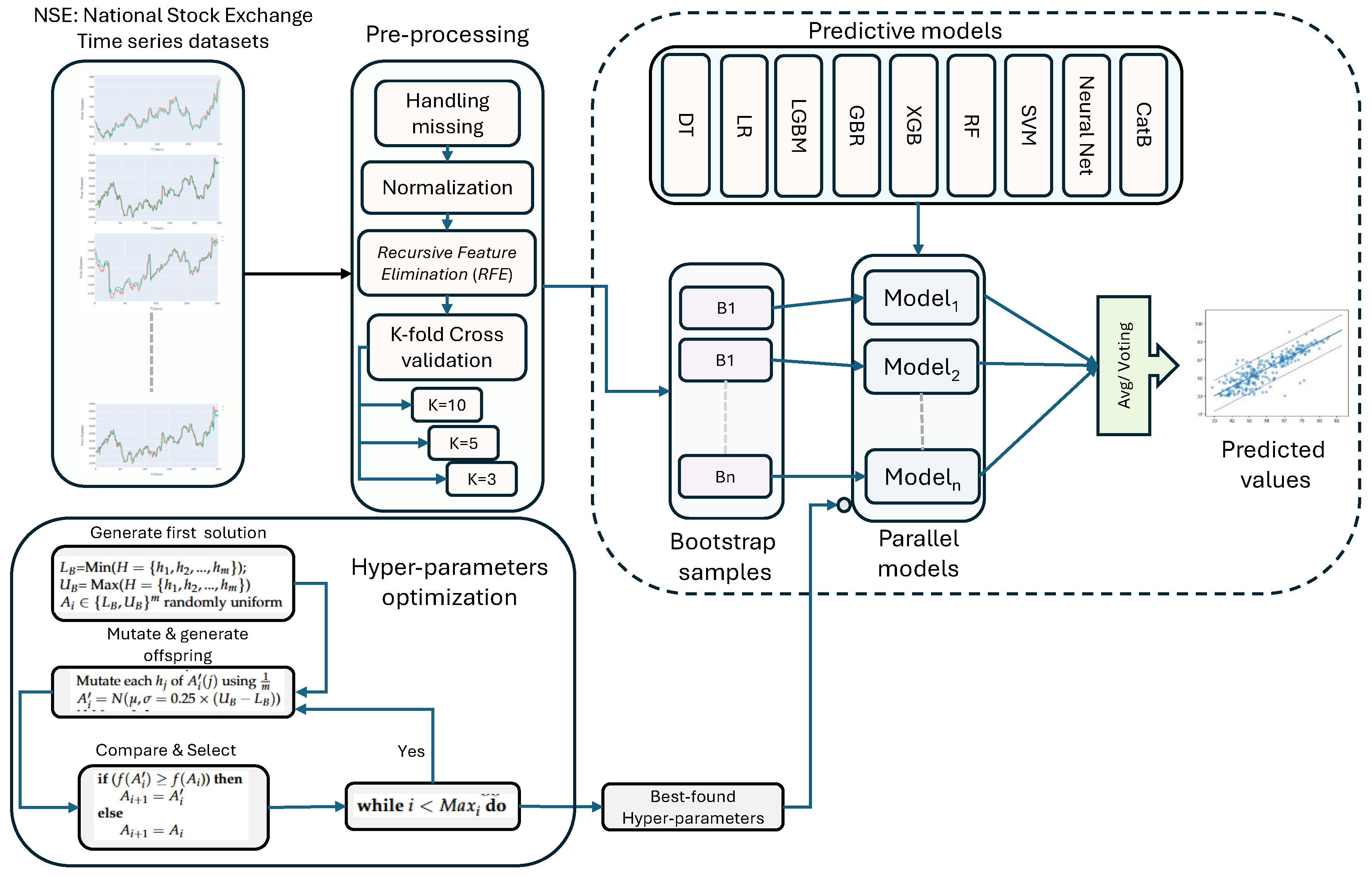
Figure 6.
Year Wise No. of Trading Days.
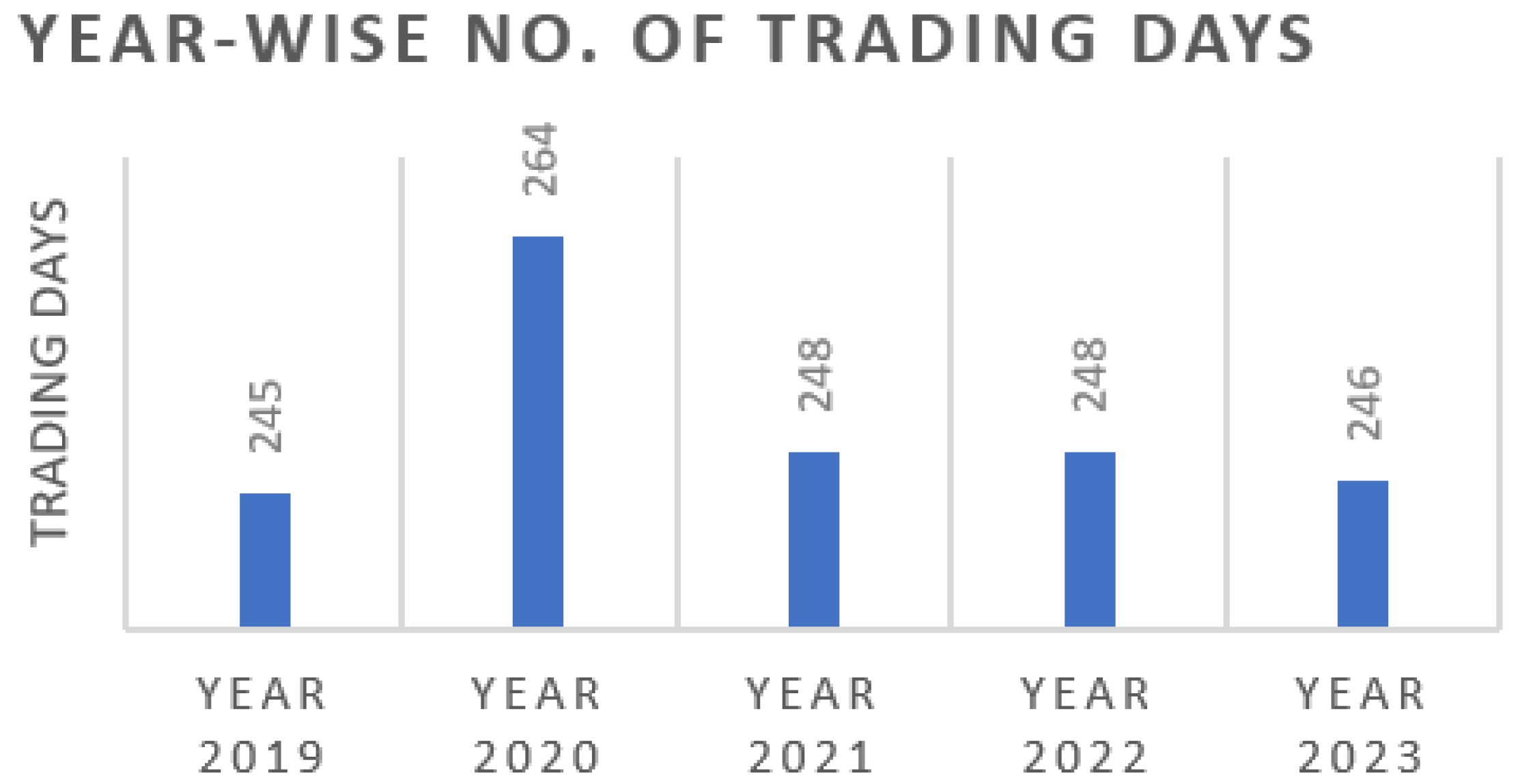
Figure 7.
Working of Recursive Feature Elimination.
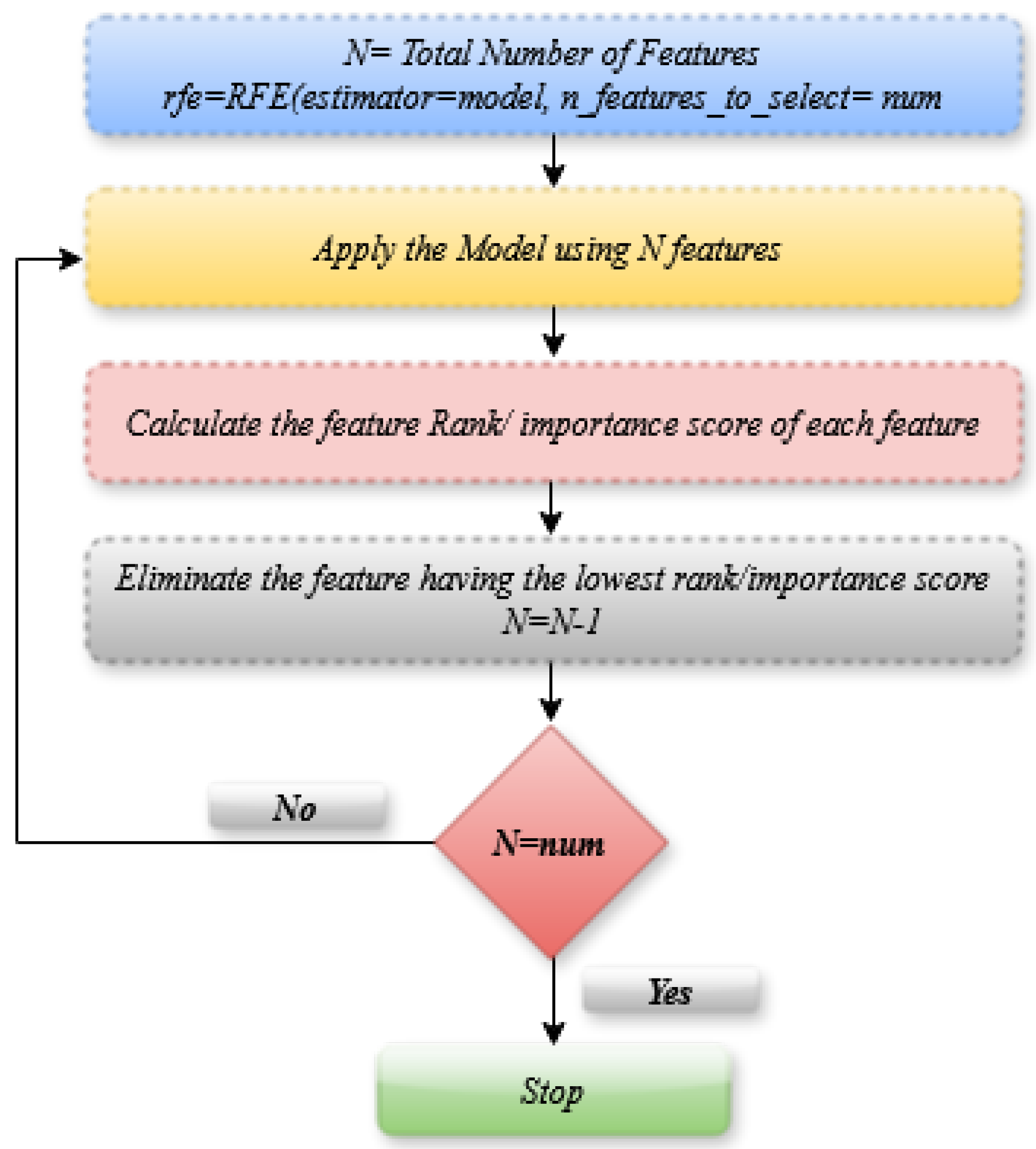
Figure 8.
Comparative line chart between actual and predicted price using different ML approaches.
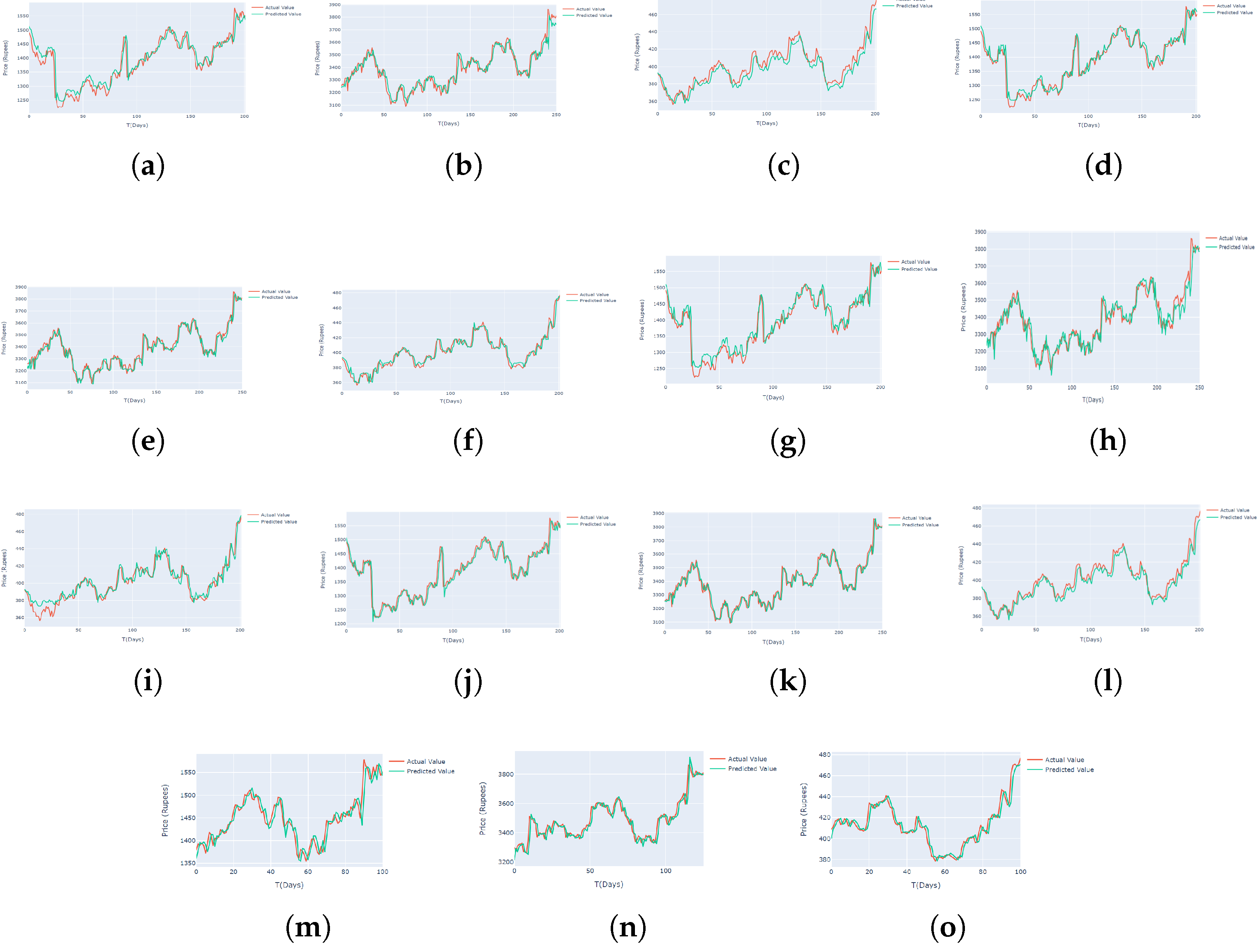
Figure 9.
Comparison of proposed ML Approaches based on MAPE and R Square on Infosys, TCS, and Wipro.
Figure 9.
Comparison of proposed ML Approaches based on MAPE and R Square on Infosys, TCS, and Wipro.
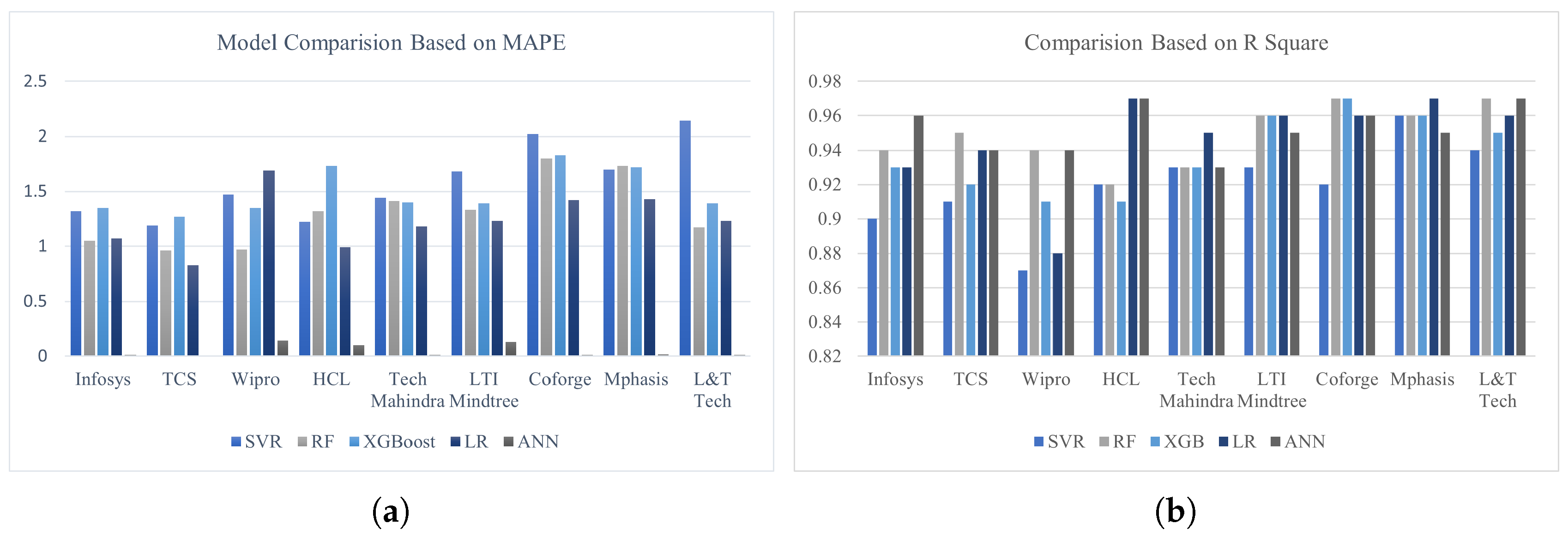
Figure 10.
Comparison of proposed ML Approaches based on RMSE and MAE on Infosys, TCS, and Wipro.
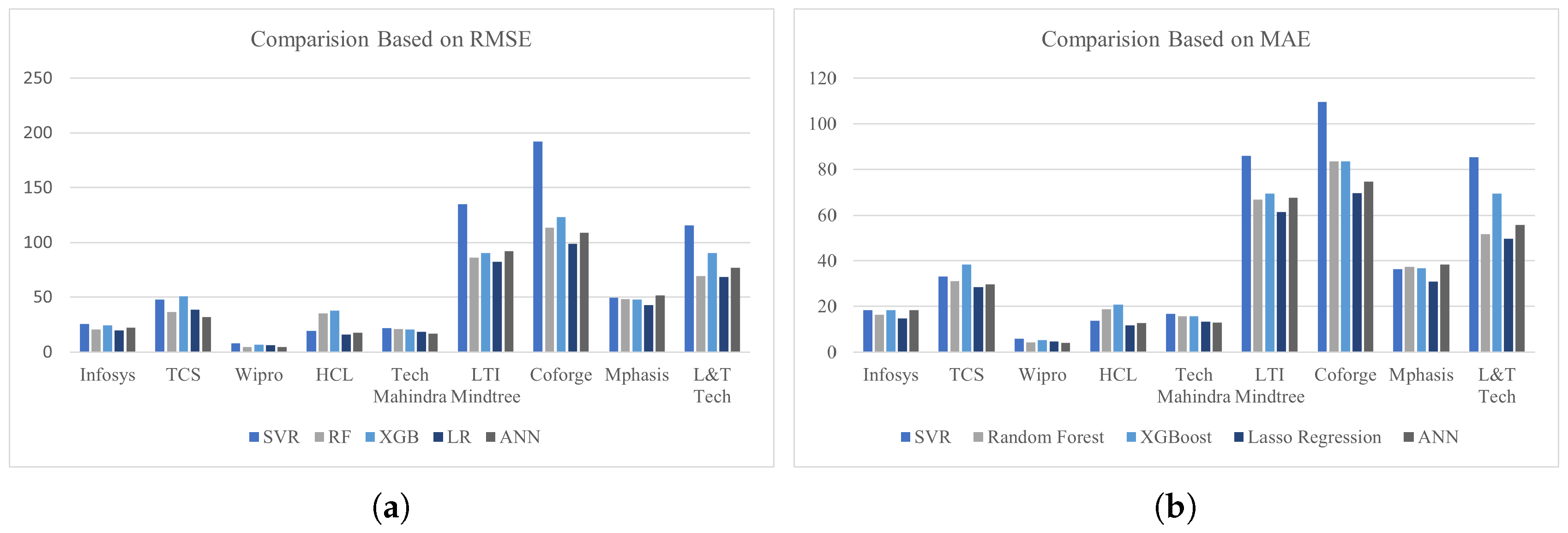
Figure 11.
Statistical results of Bagging ensemble models performance for nine NSE datasets based on .
Figure 11.
Statistical results of Bagging ensemble models performance for nine NSE datasets based on .
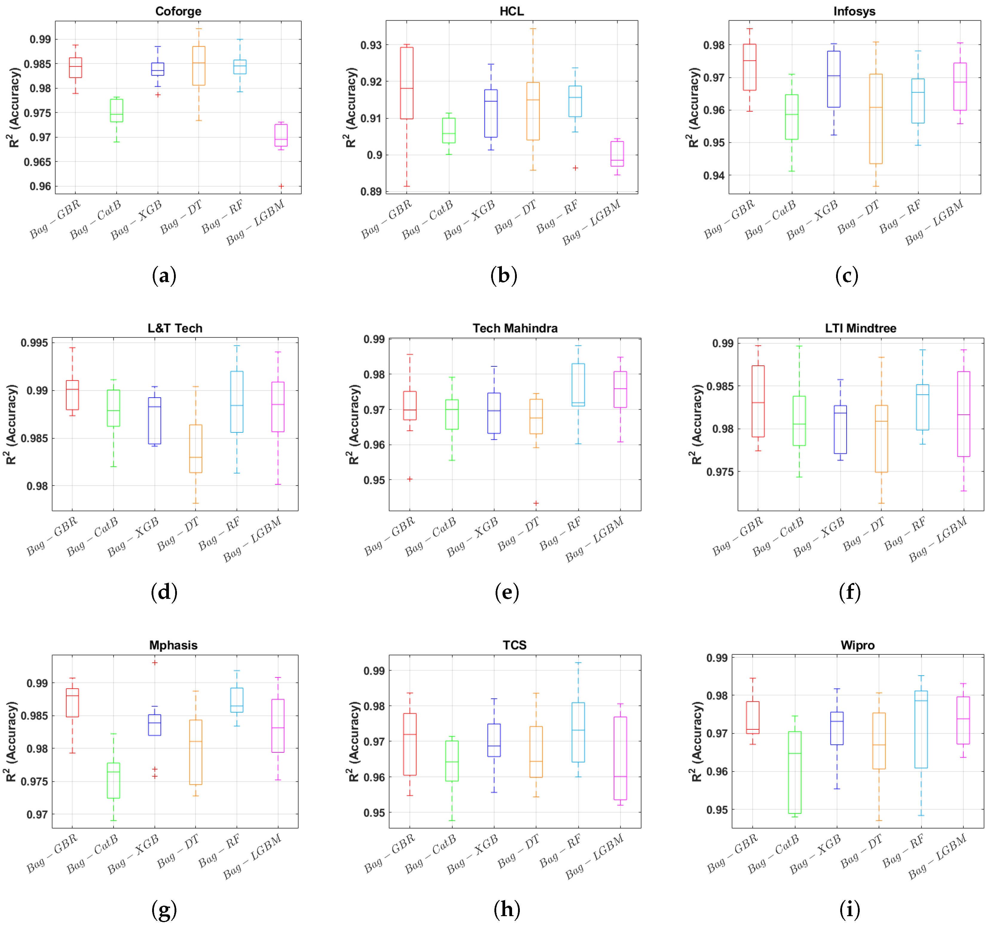
Figure 12.
Statistical results of Bagging ensemble models performance for nine NSE datasets based on MAE.
Figure 12.
Statistical results of Bagging ensemble models performance for nine NSE datasets based on MAE.
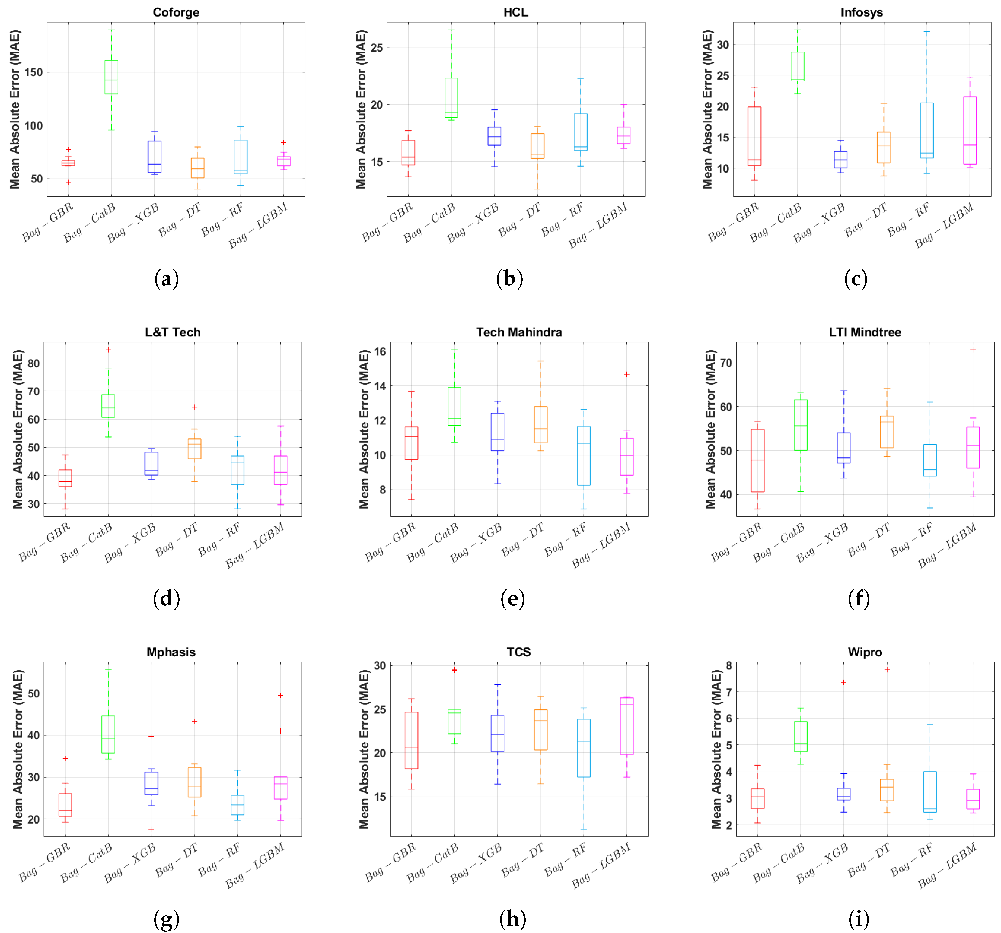
Table 1.
Summarized studies of various machine learning approaches applied in stock market prediction.
Table 1.
Summarized studies of various machine learning approaches applied in stock market prediction.
| Ref | Dataset | Objective of the study | Technique | Evaluation Metrics | Conclusion |
|---|---|---|---|---|---|
| [32] | 24 stocks were selected from the Shanghai Stock Exchange (SSE) 50 index | Portfolio construction using ML approach. First, the stock price prediction and then portfolio selection was performed | Hybrid model XGBoost + Improved Firefly (IFA) was developed | — | In terms of risks and returns, the suggested strategy outperforms benchmarks and conventional approaches |
| [33] | NSE Index NIFTY-50 from the period March 2022 to March 2023 was used for experimentation | Comparative analysis of various machine learning approaches in predicting stock prices. | RF, SVR, Ridge, Lasso Regression and KNN model | MAE R2 | SVR outperformed all other approaches |
| [34] | Data was collected from the Amadeus Database which provides financial information across Europe. | Aim to predict the market’s direction one year ahead. Comparative analysis between various ensemble and single classifier models has been done | Ensemble approaches: RF, AdaBoost, and Kernel Factory Single classifier approach: ANN, LR, KNN and SVM | ROC-AUC | An ensemble approach RF is observed the top performer among all these seven techniques. In the case of High-Frequency Trading (HFT), the results are not generalizable, which is the main limitation of this study. |
| [35] | Randomly sampled ten stocks having ticker symbols as AAPL, AMS, AMZN, FB, MSFT, NKE, SNE, TATA, TWTR, and TYO were selected for the experimental evaluation. | Prediction of stock direction with different trading window sizes | RF and XGB were employed in this study. Six technical indicators (RSI, SO, W%R, MACD, PROC, OBV)1 were computed from the closing price and used for prediction | Accuracy, Precision, Recall, F-Score Specificity, AUC, Brier Score | By increasing the width of the trading window accuracy and F-score also increases. The selection of appropriate technical indicators also impacts the performance of the model. |
| [36] | Two years of NASDAQ data have been used | Prediction of daily closing price | ANN has been applied. Min-Max approach has been used for data scaling | MSE | The suggested approach achieved acceptable results and reduced the error rate to less than 2%. |
| [37] | Four categories of data, including basic data, trading data, finance data, and other reference data, were collected from the Chinese Stock Market. | Examine the various effective approaches like feature engineering, financial domain knowledge, and prediction algorithms for short-term trend prediction. | LSTM is applied to predict price trends. | Accuracy, Precision, Recall | PCA significantly enhances the performance of the LSTM model and reduces training time. |
| [38] | Dataset of ISE2-30 were collected. Technical indicators including MA14, MA37 %K14, %D3, and RSI14 were computed for the development of a better prediction system | Future stock market trend prediction | Eight Neural Networks and a Logistic Regression (LR) approaches have been employed. | Accuracy | ANN gives better results by using %K14, %D3, and RSI14 simultaneously as compared to LR. |
| [39] | Apple, Amazon Google, Tesla, Netflix, BEXIMCO Pharmaceutical | Short term and Long Term stock price movement prediction | Simple Moving Average (SMA), Exponential Moving Average (EMA) and LSTM | RMSE, MAPE | In Short-Term prediction, LSTM is the top performer and it has been seen for Long-Term prediction the performance of LSTM has fallen in contrast to SMA and EMA |
| [40] | 10-year data of the petroleum, Diversified financials, non-metallic minerals, and basic metals were collected from the TSE3. Two methods to input the information: continuous and binary | Prediction of stock market movement using ML and DL approaches. Two methods, continuous and binary, were used to input the information. | Nine ML methods, namely DT, RF, AdaBoost, XGBoost, SVC, Naïve Bayes, KNN, LR, and ANN and two Deep Learning approaches, RNN and LSTM, were applied. | F1 Score Accuracy ROC-AUC | ML approaches show significant improvement with binary data as compared to continuous data. Indeed both deep learning methods (RNN and LSTM) achieved better results in both types of data. |
| [41] | Daily prices of Coca-Cola, Cisco Systems, Nike, and Goldman Sacks were selected. | Development of a deep learning approach for the prediction of stock price changes based on past changes | Analysis of various neural network approaches, including MLP, CNN, and LSTM. | AUC | Prediction of significant changes in the field of stock market can be achieved with a high degree of accuracy |
| [42] | NSE, BSE, NYSE, NASDAQ, S&P 500, Dow Jones, and Nikkei 225 | To analyze the stock price variations of highly volatile and nonlinear stocks for the year 2020 in order to avoid financial loss of investors | LSTM with adam optimizer and sigmoid activation function | MAPE | From experimental analysis, it is interpreted that fluctuations of stock prices have a significant impact on the MAPE score |
| [43] | Intel Corporation, Indian Oil Corporation, NTPC Limited, Citigroup, GF Securities, and Google | To perform next day’s opening price prediction using five Technical Indicators (TIs) in addition to OHLC data | GRU & LSTM were applied | MAPE, MAE, R-Square, RMSE, and MDA (Mean Directional Accuracy) | The forecasting precision of the proposed approaches has been significantly improved by using TI’s. GRU model shows remarkable predictive ability when contrasted with LSTM network model. |
| [44] | HPQ, Bank of New York, and Pfizer | Presented single layered DL model with a global pooling mechanism that is computationally efficient in performing stock closing price prediction | Vanila LSTM, stacked LSTM & Bi-LSTM were applied | RMSE, MAE, and R-Square | Among three variants of LSTM, Bi-LSTM especially when optimized using RMSprop consistently performed better than the other two versions across a variety of datasets. |
Table 3.
Performance of SVR on top IT Sector Stocks.
| Data Partitioning | 70:30 | 80:20 | 90:10 | |||||||||
| Evaluation metric | MAPE | R2 | RMSE | MAE | MAPE | R2 | RMSE | MAE | MAPE | R2 | RMSE | MAE |
| Infosys | 1.42 | 0.93 | 27.21 | 20.66 | 1.32 | 0.90 | 26.12 | 18.39 | 1.07 | 0.83 | 21.41 | 15.81 |
| TCS | 1.59 | 0.90 | 52.08 | 38.33 | 1.19 | 0.91 | 47.65 | 33.18 | 1.03 | 0.83 | 56.02 | 36.63 |
| Wipro | 1.37 | 0.85 | 7.51 | 5.54 | 1.47 | 0.87 | 8.02 | 5.94 | 1.32 | 0.86 | 8.01 | 5.58 |
| HCL | 1.25 | 0.95 | 21.41 | 15.22 | 1.22 | 0.92 | 19.53 | 13.89 | 1.51 | 0.92 | 26.90 | 19.55 |
| Tech Mahindra | 1.76 | 0.91 | 24.37 | 19.25 | 1.44 | 0.93 | 22.32 | 16.65 | 1.50 | 0.87 | 23.24 | 18.24 |
| LTI Mindtree | 2.34 | 0.88 | 151.49 | 111.33 | 1.68 | 0.93 | 135.28 | 85.90 | 1.94 | 0.87 | 167.83 | 105.29 |
| Coforge | 2.15 | 0.90 | 202 | 120.82 | 2.02 | 0.92 | 192.02 | 109.52 | 2.52 | 0.87 | 219.01 | 137.94 |
| Mphasis | 2.20 | 0.92 | 60.02 | 46.30 | 1.70 | 0.96 | 49.73 | 36.39 | 1.67 | 0.92 | 53.85 | 38.81 |
| L&T Tech | 2.48 | 0.93 | 125.37 | 95.97 | 2.14 | 0.94 | 115.87 | 85.42 | 2.55 | 0.84 | 143.43 | 117.74 |
Table 4.
Performance of Random Forest on Top IT Sector Stocks.
| Data Partitioning | 70:30 | 80:20 | 90:10 | |||||||||
| Evaluation metric | MAPE | R2 | RMSE | MAE | MAPE | R2 | RMSE | MAE | MAPE | R2 | RMSE | MAE |
| Infosys | 1.21 | 0.94 | 23.51 | 17.52 | 1.05 | 0.94 | 20.80 | 16.36 | 1.05 | 0.85 | 20.75 | 17.02 |
| TCS | 1.01 | 0.93 | 44.79 | 33.68 | 0.96 | 0.95 | 36.64 | 31.11 | 1.03 | 0.88 | 48.94 | 36.17 |
| Wipro | 1.20 | 0.89 | 6.29 | 4.76 | 0.97 | 0.94 | 4.90 | 4.31 | 1.06 | 0.91 | 6.45 | 4.44 |
| HCL | 1.58 | 0.86 | 38.58 | 19.94 | 1.32 | 0.92 | 35.22 | 18.64 | 2.04 | 0.79 | 51.77 | 27.59 |
| Tech Mahindra | 1.41 | 0.93 | 21.75 | 16.25 | 1.41 | 0.93 | 21.10 | 15.72 | 1.59 | 0.86 | 23.11 | 18.99 |
| LTI Mindtree | 1.62 | 0.94 | 102.65 | 78.14 | 1.33 | 0.96 | 86.31 | 66.81 | 1.34 | 0.93 | 89.11 | 71.61 |
| Coforge | 1.85 | 0.96 | 121.51 | 87.31 | 1.80 | 0.97 | 113.78 | 83.53 | 1.90 | 0.89 | 144.14 | 101.44 |
| Mphasis | 2.09 | 0.93 | 56.35 | 44.58 | 1.73 | 0.96 | 48.33 | 37.29 | 1.79 | 0.92 | 53.90 | 42.13 |
| L&T Tech | 1.66 | 0.96 | 86.20 | 64.17 | 1.17 | 0.97 | 69.32 | 51.76 | 1.45 | 0.94 | 84.36 | 65.12 |
Table 5.
Performance of XGBoost on top IT Sector Stocks.
| Data Partitioning | 70:30 | 80:20 | 90:10 | |||||||||
| Evaluation metric | MAPE | R2 | RMSE | MAE | MAPE | R2 | RMSE | MAE | MAPE | R2 | RMSE | MAE |
| Infosys | 1.37 | 0.92 | 24.36 | 18.16 | 1.35 | 0.93 | 24.85 | 18.37 | 1.50 | 0.85 | 21.15 | 15.61 |
| TCS | 1.02 | 0.93 | 48.40 | 33.84 | 1.27 | 0.92 | 50.90 | 38.37 | 0.99 | 0.90 | 43.37 | 31.76 |
| Wipro | 1.59 | 0.85 | 7.55 | 5.81 | 1.35 | 0.91 | 7.06 | 5.30 | 1.44 | 0.88 | 7.44 | 6.00 |
| HCL | 1.83 | 0.83 | 43.47 | 23.16 | 1.73 | 0.91 | 37.88 | 20.65 | 2.38 | 0.75 | 59.96 | 32.20 |
| Tech Mahindra | 1.46 | 0.92 | 22.54 | 16.76 | 1.40 | 0.93 | 20.82 | 15.73 | 2.20 | 0.64 | 34.18 | 27.61 |
| LTI Mindtree | 2.10 | 0.91 | 131.84 | 101.52 | 1.39 | 0.96 | 90.48 | 69.45 | 1.53 | 0.91 | 103.49 | 81.37 |
| Coforge | 2.02 | 0.94 | 150.32 | 100.71 | 1.83 | 0.97 | 123.37 | 83.43 | 2.39 | 0.88 | 200.62 | 134.11 |
| Mphasis | 5.93 | 0.66 | 141.54 | 118.43 | 1.72 | 0.96 | 47.76 | 36.68 | 2.09 | 0.90 | 62.07 | 48.60 |
| L&T Tech | 2.10 | 0.89 | 131.84 | 101.52 | 1.39 | 0.95 | 90.48 | 69.45 | 1.51 | 0.91 | 103.49 | 81.37 |
Table 6.
Performance of Lasso Regression on top IT Sector Stocks.
| Data Partitioning | 70:30 | 80:20 | 90:10 | |||||||||
| Evaluation metric | MAPE | R2 | RMSE | MAE | MAPE | R2 | RMSE | MAE | MAPE | R2 | RMSE | MAE |
| Infosys | 1.08 | 0.95 | 21.75 | 15.60 | 1.07 | 0.93 | 20.05 | 14.87 | 0.95 | 0.87 | 18.78 | 13.89 |
| TCS | 0.89 | 0.94 | 40.49 | 29.78 | 0.83 | 0.94 | 38.59 | 28.34 | 0.83 | 0.90 | 42.36 | 29.29 |
| Wipro | 1.21 | 0.89 | 6.29 | 4.56 | 1.69 | 0.88 | 6.63 | 4.84 | 1.26 | 0.92 | 6.48 | 4.33 |
| HCL | 1.04 | 0.96 | 15.993 | 11.61 | 0.99 | 0.97 | 16.37 | 11.84 | 1.02 | 0.96 | 18.92 | 13.02 |
| Tech Mahindra | 1.28 | 0.94 | 19.30 | 14.16 | 1.18 | 0.95 | 18.61 | 13.46 | 1.44 | 0.87 | 18.64 | 13.78 |
| LTI Mindtree | 1.42 | 0.96 | 91.03 | 68.51 | 1.23 | 0.96 | 82.61 | 61.52 | 1.82 | 0.94 | 79.20 | 57.93 |
| Coforge | 1.52 | 0.95 | 99.37 | 76.75 | 1.42 | 0.96 | 98.92 | 69.65 | 1.59 | 0.94 | 107.88 | 72.98 |
| Mphasis | 1.47 | 0.96 | 42.43 | 31.57 | 1.43 | 0.97 | 42.62 | 30.85 | 1.55 | 0.93 | 48.84 | 36.32 |
| L&T Tech | 1.43 | 0.94 | 74.42 | 53.42 | 1.23 | 0.96 | 68.57 | 49.75 | 1.32 | 0.94 | 0.69 | 50.92 |
Table 7.
Performance of ANN on top IT Sector Stocks dataset.
| Data Partitioning | 70:30 | 80:20 | 90:10 | |||||||||
| Evaluation metric | MAPE | R2 | RMSE | MAE | MAPE | R2 | RMSE | MAE | MAPE | R2 | RMSE | MAE |
| Infosys | 0.014 | 0.93 | 26.79 | 20.12 | 0.013 | 0.96 | 22.63 | 18.39 | 0.04 | 0.91 | 26.32 | 21.14 |
| TCS | 0.0099 | 0.92 | 25.79 | 33.68 | 0.0089 | 0.94 | 32.33 | 29.58 | 0.0094 | 0.93 | 46.87 | 31.58 |
| Wipro | 0.016 | 0.89 | 6.57 | 4.68 | 0.014 | 0.94 | 4.85 | 4.11 | 0.019 | 0.92 | 6.60 | 4.68 |
| HCL | 0.010 | 0.95 | 19.74 | 13.84 | 0.10 | 0.97 | 18.04 | 12.93 | 0.011 | 0.91 | 22.83 | 15.43 |
| Tech Mahindra | 0.012 | 0.86 | 19.39 | 14.07 | 0.011 | 0.93 | 17.21 | 13.10 | 0.011 | 0.87 | 17.94 | 13.30 |
| LTI Mindtree | 0.013 | 0.92 | 97.56 | 73.95 | 0.013 | 0.95 | 91.97 | 67.77 | 0.012 | 0.93 | 92.18 | 66.84 |
| Coforge | 0.016 | 0.94 | 115.38 | 82.38 | 0.013 | 0.96 | 109.01 | 74.59 | 0.014 | 0.93 | 123.56 | 81.02 |
| Mphasis | 0.019 | 0.92 | 56.96 | 42.88 | 0.016 | 0.95 | 51.84 | 38.31 | 0.016 | 0.91 | 54.22 | 39.11 |
| L&T Tech | 0.013 | 0.95 | 80.17 | 60.07 | 0.013 | 0.97 | 76.89 | 55.78 | 0.014 | 0.93 | 89.69 | 66.92 |
Table 11.
The performance of Bagging ensemble models trained and tested by Coforge dataset.
| Bag-GBR | Bag-CatB | ||||||||||||
| Metric | RMSE | MAE | R2 | MSLE | EVS | SMAPE | Metric | RMSE | MAE | R2 | MSLE | EVS | SMAPE |
| Mean | 100.938 | 64.378 | 0.984 | 3.54E-04 | 0.980 | 1.294 | Mean | 205.939 | 145.449 | 0.975 | 1.49E-03 | 0.944 | 2.886 |
| Min | 77.708 | 46.616 | 0.979 | 2.03E-04 | 0.974 | 0.936 | Min | 149.168 | 95.452 | 0.969 | 7.37E-04 | 0.926 | 1.883 |
| Max | 116.047 | 77.434 | 0.989 | 4.81E-04 | 0.987 | 1.568 | Max | 256.288 | 189.583 | 0.978 | 2.32E-03 | 0.963 | 3.777 |
| STD | 9.846 | 7.788 | 0.003 | 7.03E-05 | 0.003 | 0.159 | STD | 30.104 | 26.197 | 0.003 | 4.44E-04 | 0.011 | 0.525 |
| Bag-XGB | Bag-DT | ||||||||||||
| Metric | RMSE | MAE | R2 | MSLE | EVS | SMAPE | Metric | RMSE | MAE | R2 | MSLE | EVS | SMAPE |
| Mean | 106.100 | 68.973 | 0.984 | 4.01E-04 | 0.979 | 1.393 | Mean | 89.655 | 59.760 | 0.985 | 3.01E-04 | 0.983 | 1.224 |
| Min | 87.797 | 53.927 | 0.979 | 2.69E-04 | 0.971 | 1.095 | Min | 65.135 | 40.200 | 0.973 | 1.41E-04 | 0.968 | 0.808 |
| Max | 138.063 | 94.271 | 0.989 | 6.51E-04 | 0.984 | 1.880 | Max | 120.208 | 79.706 | 0.992 | 5.25E-04 | 0.991 | 1.637 |
| STD | 17.845 | 14.700 | 0.003 | 1.37E-04 | 0.004 | 0.289 | STD | 15.974 | 12.344 | 0.006 | 1.16E-04 | 0.007 | 0.262 |
| Bag-RF | Bag-LGBM | ||||||||||||
| Metric | RMSE | MAE | R2 | MSLE | EVS | SMAPE | Metric | RMSE | MAE | R2 | MSLE | EVS | SMAPE |
| Mean | 101.850 | 65.997 | 0.984 | 3.79E-04 | 0.981 | 1.336 | Mean | 127.512 | 68.004 | 0.969 | 5.17E-04 | 0.966 | 1.345 |
| Min | 77.221 | 43.579 | 0.979 | 1.92E-04 | 0.971 | 0.871 | Min | 118.512 | 58.441 | 0.960 | 4.27E-04 | 0.957 | 1.143 |
| Max | 140.132 | 98.873 | 0.990 | 7.12E-04 | 0.988 | 2.008 | Max | 142.817 | 83.664 | 0.973 | 6.84E-04 | 0.970 | 1.676 |
| STD | 22.235 | 18.787 | 0.003 | 1.79E-04 | 0.005 | 0.380 | STD | 7.058 | 7.500 | 0.004 | 7.47E-05 | 0.004 | 0.159 |
Table 12.
Comparison of Bagging ensemble models performance trained and tested by L&T Tech dataset.
| Bag-GBR | Bag-CatB | ||||||||||||
| Metric | RMSE | MAE | R2 | MSLE | EVS | SMAPE | Metric | RMSE | MAE | R2 | MSLE | EVS | SMAPE |
| Mean | 65.882 | 50.526 | 0.984 | 2.62E-04 | 0.983 | 1.235 | Mean | 85.508 | 65.929 | 0.987 | 3.95E-04 | 0.982 | 1.569 |
| Min | 49.867 | 37.859 | 0.978 | 1.46E-04 | 0.978 | 0.922 | Min | 71.427 | 53.682 | 0.982 | 2.73E-04 | 0.974 | 1.279 |
| Max | 83.880 | 64.395 | 0.990 | 4.11E-04 | 0.990 | 1.576 | Max | 104.814 | 84.718 | 0.991 | 5.85E-04 | 0.987 | 2.017 |
| STD | 9.397 | 7.236 | 0.004 | 7.42E-05 | 0.004 | 0.178 | STD | 10.803 | 9.610 | 0.003 | 9.81E-05 | 0.004 | 0.226 |
| Bag-XGB | Bag-DT | ||||||||||||
| Metric | RMSE | MAE | R2 | MSLE | EVS | SMAPE | Metric | RMSE | MAE | R2 | MSLE | EVS | SMAPE |
| Mean | 58.092 | 43.804 | 0.987 | 2.02E-04 | 0.987 | 1.072 | Mean | 65.882 | 50.526 | 0.984 | 2.62E-04 | 0.983 | 1.235 |
| Min | 50.957 | 38.588 | 0.984 | 1.53E-04 | 0.984 | 0.943 | Min | 49.867 | 37.859 | 0.978 | 1.46E-04 | 0.978 | 0.922 |
| Max | 65.611 | 49.534 | 0.990 | 2.57E-04 | 0.990 | 1.215 | Max | 83.880 | 64.395 | 0.990 | 4.11E-04 | 0.990 | 1.576 |
| STD | 5.847 | 4.333 | 0.003 | 4.05E-05 | 0.002 | 0.106 | STD | 9.397 | 7.236 | 0.004 | 7.42E-05 | 0.004 | 0.178 |
| Bag-RF | Bag-LGBM | ||||||||||||
| Metric | RMSE | MAE | R2 | MSLE | EVS | SMAPE | Metric | RMSE | MAE | R2 | MSLE | EVS | SMAPE |
| Mean | 55.612 | 42.034 | 0.988 | 1.88E-04 | 0.988 | 1.025 | Mean | 55.633 | 42.124 | 0.988 | 1.94E-04 | 0.988 | 1.035 |
| Min | 37.265 | 28.219 | 0.981 | 8.31E-05 | 0.981 | 0.691 | Min | 39.557 | 29.574 | 0.980 | 9.36E-05 | 0.980 | 0.724 |
| Max | 70.916 | 53.880 | 0.995 | 2.98E-04 | 0.995 | 1.317 | Max | 74.546 | 57.639 | 0.994 | 3.64E-04 | 0.994 | 1.452 |
| STD | 10.168 | 7.839 | 0.004 | 6.46E-05 | 0.004 | 0.191 | STD | 11.016 | 8.582 | 0.004 | 8.22E-05 | 0.005 | 0.219 |
Disclaimer/Publisher’s Note: The statements, opinions and data contained in all publications are solely those of the individual author(s) and contributor(s) and not of MDPI and/or the editor(s). MDPI and/or the editor(s) disclaim responsibility for any injury to people or property resulting from any ideas, methods, instructions or products referred to in the content. |
© 2024 by the authors. Licensee MDPI, Basel, Switzerland. This article is an open access article distributed under the terms and conditions of the Creative Commons Attribution (CC BY) license (http://creativecommons.org/licenses/by/4.0/).
Copyright: This open access article is published under a Creative Commons CC BY 4.0 license, which permit the free download, distribution, and reuse, provided that the author and preprint are cited in any reuse.


