Transfinite Patches for Isogeometric Analysis

Christopher Provatidis

doi:10.20944/preprints202412.1721.v1

Preprint

Article

Transfinite Patches for Isogeometric Analysis

This version is not peer-reviewed.

Christopher Provatidis^*

This version is not peer-reviewed.

Downloads

Views

Comments

Submitted:

19 December 2024

Posted:

20 December 2024

You are already at the latest version

A peer-reviewed article of this preprint also exists.

Abstract

This paper extends the well-known transfinite interpolation formula, which was developed in late sixties by the applied mathematician William Gordon at the premises of General Motors as an extension of the pre-existed Coons interpolation formula. Here, a conjecture is formulated, which claims that the meaning of the involved blending functions can be enlarged, so that to include any linear independent and complete set of functions, including piecewise-linear, trigonometric functions, Bernstein polynomials, B-splines, NURBS and so on. In this sense, NURBS-based isogeometric analysis and aspects of T-splines may be considered as special cases. Applications are provided for the accuracy in the interpolation through the L2-error norm, of closed-formed functions prescribed at the nodal points of the transfinite patch, which represent the solution of partial differential equations under boundary conditions of Dirichlet type.

Keywords:

interpolation

;

approximation

;

isogeometric analysis

;

B-splines

;

NURBS

;

T-splines

Subject:

Computer Science and Mathematics - Applied Mathematics

MSC: 65N06; 65B99

1. Introduction

Classical textbooks in computer-aided geometric design (CAGD) [1, 2], suggest that one of the first CAGD formulations in Computational Geometry is the Coons’ interpolation formula [3]. Despite its high historical importance, we could say that the latter is merely the extension of the linear interpolation in two-dimensional quadrilateral domains (patches). Even in the first Coons’ report [3], it is clearly written that this interpolation refers to both the geometry of a patch as well as to the estimation of a function U(x,y) when its values are prescribed along the four edges of a quadrilateral patch ABCD.

The disadvantage of Coons’ interpolation formula is its incapability of considering information related to inner points. For example, if the values of the function U(x,y) vanish on the entire boundary, then Coons’ interpolation formula will provide zero values everywhere in the domain ABCD. This shortcoming was resolved by William Gordon at General Motors Research Laboratories (GMRL), who proposed that information may be given of course along the boundary (as also happened with Coons’ interpolation) but also along internal lines parallel to the edges of the quadrilateral patch (sometimes called inter-boundaries or stations). In more detail, Gordon preserved the meaning of blending functions, which had been previously proposed by Coons, but extended it to include the inter-boundaries as well [4-7].

It is worth mentioning that the same team at GMRL applied Coons’ interpolation for the implementation of the Ritz-Galerkin method to the numerical solution of a boundary value problem (BVP) regarding Laplace equation within a complex domain in the form of a five-sided patch [8]. This fact can be rephrased as follows. The utilization of the same global interpolation (within the entire patch) for both the geometry and the numerical approximation of the solution were proposed for the first time by the GMRL group, for practical engineering purposes. This is simply the isoparametric consideration, well known in finite element analysis, in which the global trial function was taken equal to that which describes the geometry of the geometric patch.

The few papers published by the abovementioned GMRL group were written in a very dense style, so their decryption was not fully performed widely. The impression a reader takes from their reading is that the blending functions must be Lagrange polynomials which vanish at the internal stations, whereas as the trial functions along them may be either Lagrange polynomials or Hermite splines. The latest papers published by the GMRL group on this issue are [9,10].

For over thirty years, the above idea of using the same CAGD-based interpolation for both the geometry and the physical function U(x,y), which is involved into the governing PDE D(u) – f = 0, did not attract much attention [11-13], until the advent of the so-called isogeometric analysis (IGA), which changed the establishment [14,15]. In [15](p.8), it is recognized that the same interpolation was used in Coons and transfinite elements as well, but IGA dominated because it closely follows the most recent rules of CAGD-theory in which the shape remains unaltered after knot insertion, degree elevation, or any combination of them. The history of implementing transfinite interpolation, as an alternative to FEM, includes a volume of 60 papers written from 1989 till 2018, of which the resumé has been included in a monograph published in 2019 by Provatidis [16].

Although there is no doubt that IGA is an extraordinary technique itself, this paper shows that it can be considered as a particular case of transfinite interpolation. Clearly, transfinite interpolation is a superset of tensor-product Lagrange polynomials, tensor-product Bernstein polynomials, tensor-product B-splines, and tensor-product NURBS. The novel key point to this consideration is to revise the meaning of the so-called blending functions including non-cardinal sets as well, and thus to obtain hybrid schemes, with the same or different functional sets within the transfinite element which describes an entire quadrilateral patch. Preliminary but rather empirical thoughts on this issue have been recently presented in Ref. [17]. In the present paper a new conjecture is proposed.

The paper is structured as follows. In section 2 we begin with the classical linear blending functions which are involved in Coons’ interpolation formula and discuss the meaning of the three projectors involved in the Boolean sum. In section 3 we continue with higher-order blending functions which are involved in Gordon’s transfinite interpolation formula, explain the meaning of the stations, and prove that the tensor product is a special case. In section 4 we present the most useful univariate functions, which may play the role of either a blending or a trial function. In section 5 we show that the non-rational tensor-product Bernstein polynomials is an equivalent tensor-product Lagrange polynomials, and we provide a formula for the determination of the α-coefficients therein. In section 6 we show that the tensor-product B-splines are produced using B-splines for both the blending and trial functions. Based on this finding, we further conjecture the utilization for blending functions, of any linear independent and complete functional set, including non-cardinal (de Boor) B-splines and NURBS. In section 7 we present variations of unstructured transfinite elements. In section 8 we discuss mesh refinement using a single element, whereas in section 9 we deal with some simple T-spline elements. In general, except for finding the closed-form analytical expressions, we also interpolate within numerous transfinite macro-elements under given boundary conditions of Dirichlet type and determine the L2-error norm.

2. Linear Blending Functions in Coons’ interpolation

2.1 Linear interpolation in the physical space

Given, U₁ and U₂, which denote the values of a function U(x) the end-points of an one-dimensional interval [0,a], at any position x∈[0,a] the value of the function may be linearly interpolated by:

U(x) = (1-x/a)U₁ + (x/a)U₂.

(1)

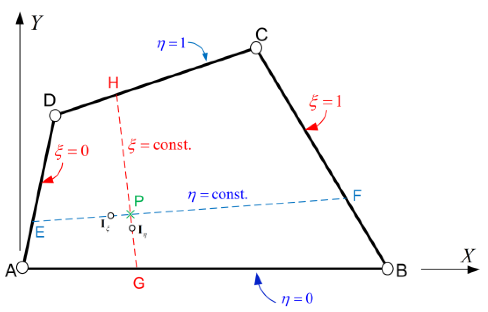
Figure 1. The quadrilateral ABCD.

Equation (1) can be extended to a rectangle [0,a] × [0,b], considering the tensor product, i.e., through the expression:

U(x) = (1-x/a)(1-y/b)U₁ + (x/a)(1-y/b)U₂ + (x/a)(y/b)U₃ + (1-x/a)(y/b)U₄.

(2)

2.2. Linear interpolation in the parametric space

If the position x∈[0,a] is normalized to its length ’a’ by introducing the parameter:

ξ = x/a,

(3)

so that ξ∈[0,1], Equation (1) is re-written as follows:

U(x) = (1-ξ)U₁ + ξU₂.

(4)

Moreover, regarding the above rectangle [0,a] × [0,b], the position (x,y) within it can be normalized, so as the x-coordinate is replaced according to Equation (3), whereas the y-coordinate is also normalized as:

η = y/b.

(5)

Then, Equation (2) is re-written as:

U(x) = (1-ξ)(1-η)U₁ + ξ(1-η)U₂ + ξηU₃ + (1-ξ)ηU₄.

(6)

2.3. Projectors within a quadrilateral

Definition of parameters:

The position of a point P(x,y) within a planar quadrilateral ABCD is usually defined by its two Cartesian coordinates, x and y. Alternatively, the same point P(ξ,η) can be uniquely determined using two parameters, ξ and η.

When the quadrilateral is rectangular and the axis origin is at corner A, the definition of the parameters (ξ,η) is direct, according to Equation (3) and Equation (5).

In general, given the parameter ξ, we define the unique points E and F on the edges AD and BC (see, Figure 1), respectively, so that:

AE/AD = BF/BC = ξ.

(7)

The points E and F, which divide the opposite edges AD and BC in the same ratio ξ according to Equation (7), are called ‘corresponding points’ in the ξ-direction.

Similarly, for the parameter η we define the unique points G and H on the edges AB and DC, respectively, so that:

AG/AB = DH/DC = η.

(8)

The points G and H, which divide the opposite edges AB and DC in the same ratio η according to Equation (8), are called ‘corresponding points’ in the η -direction.

Having determined the two couples of points, (E,F) and (G,H), the intersection of the lines EF and GH determines the unique point P(ξ,η). Inversely, for any point P internal to the quadrilateral ABCD, there is a unique line EF passing through it which intersects the opposite edges AD and BC in equal ratios, which is the parameter η. The same holds true for the intersection of the opposite edges AB and DC at the same ratio, which is the parameter ξ.

To understand the meaning of the projector P_ξ and P_η, we introduce the following Theorem-1.

Theorem-1: The point P(ξ,η) within a quadrilateral ABCD divides the segment of its corresponding points (E,F) and (G,H) into the same ratios as those on the opposite edges:

EP/EF = ξ and GP/GH = η.

(9)

Proof: Let us consider point P(x,y) within the quadrilateral ABCD. Obviously, there is a unique line passing through this point which intersects the opposite edges AD and BC at the points E and F, respectively, having the same ratio, i.e., η = AE/AD = BF/BC, according to Equation (7).

Then, the position vector of the point I_ξ which divides the segment EF into the ratio EI_ξ/EF = ξ, will be given as (see, Figure 1)

\begin{array}{l} {\vec{r}}_{I_{ξ}} & = (1 - ξ) {\vec{r}}_{E} + ξ {\vec{r}}_{F} \\ = (1 - ξ) [(1 - η) {\vec{r}}_{A} + η {\vec{r}}_{D}] + ξ [(1 - η) {\vec{r}}_{B} + η {\vec{r}}_{C}] \\ = (1 - ξ) (1 - η) {\vec{r}}_{A} + ξ (1 - η) {\vec{r}}_{B} + ξ η {\vec{r}}_{C} + (1 - ξ) η {\vec{r}}_{D} . \end{array}

(10)

Similarly, the position vector of the point I_η which divides the segment GH into the ratio E I_η /EF = η, will be given as (see, Figure 1)

\begin{array}{l} {\vec{r}}_{I_{η}} & = (1 - η) {\vec{r}}_{G} + η {\vec{r}}_{H} \\ = (1 - η) [(1 - ξ) {\vec{r}}_{A} + ξ {\vec{r}}_{B}] + η [(1 - ξ) {\vec{r}}_{D} + ξ {\vec{r}}_{C}] \\ = (1 - ξ) (1 - η) {\vec{r}}_{A} + ξ (1 - η) {\vec{r}}_{B} + ξ η {\vec{r}}_{C} + (1 - ξ) η {\vec{r}}_{D} . \end{array}

(11)

Since the right-hand sides of Equation (10) and (11) are identical, the vectors

{\vec{r}}_{I_{ξ}}

and

{\vec{r}}_{I_{η}}

must be identical, i.e.,

{\vec{r}}_{I_{ξ}} \equiv {\vec{r}}_{I_{η}}

, which means that the points I_ξ and I_η coincide (I_ξ = I_η). Therefore, since (I_ξ ∈ EF ∧ I_η ∈ GH ∧ I_ξ = I_η), we derive that either of the points (I_ξ, I_η) is the unique intersection of the lines EF and GH, which completes the proof. ■

2.4. Interpolation by a Boolean sum

The above ‘Theorem-1’ has probably inspired the so-called “Coons’ interpolation formula”, which refers to an arbitrary curvilinear patch ABCD. In general, the parameterization of this patch depends on the choice of the four corner points (A,B,C,D) on the true patch in the physical space (x,y). Given these corners, the boundary part AB defines the body-fitted (curvilinear) ξ-axis whereas the part AD defines the η-axis. Given the parameters (ξ,η), we define the points (E,F,G,H) on the edges (AD,BC,AB,DC), respectively, and then determine the abovementioned points I_ξ and I_η. In general, these two points are different (I_ξ ≠ I_η), and thus it becomes necessary to find a way to harmonize them. Note that the obvious remedy to take the mean average (I_ξ + I_η)/2 does not work well, because it cannot accurately represent the prescribed boundary conditions. The answer to this problem was given by Steven Coons in 1964, and then in his final report at MIT [3]. For the smooth transition to the problem and for the sake of completeness, we express the essence of Coons’ interpolation in the form of a modified theorem (Theorem-2).

Theorem-2: Given a parametric curvilinear patch ABCD with prescribed boundaries [U(ξ,0), U(1,η), U(ξ,1), U(0,η)], each couple of parameters (ξ,η) determines the position of a point P(ξ,η) which fulfils the boundary conditions, when we apply the following Boolean sum:

U (ξ, η) = P_{ξ} {U} + P_{η} {U} - P_{ξ η} {U} .

(12)

In terms of the definitions cited in section 2.3, the three projectors involved in Equation (12) are defined as follows [3]:

\begin{array}{l} P_{ξ} {U} = (1 - ξ) U_{E} + ξ U_{F}, \\ P_{η} {U} = (1 - η) U_{G} + η U_{H}, \\ P_{ξ η} {U} = (1 - ξ) (1 - η) U_{A} + ξ (1 - η) U_{B} + ξ η U_{C} + (1 - ξ) η U_{D} . \end{array}

(13)

The blending functions involved in Equation (13) are defined as:

\begin{array}{l} E_{0} (ξ) = (1 - ξ), E_{1} (ξ) = ξ, \\ E_{0} (η) = (1 - η), E_{1} (η) = η . \end{array}

(14)

Obviously, the blending function

E_{0} (ξ)

is associated to data along the edge AD at ξ=0, whereas

E_{1} (ξ)

is associated to data along the edge BC at ξ=1. Similarly, the blending function

E_{0} (η)

is associated with the edge AB at η=0, whereas

E_{1} (η)

is associated with the edge DC at η=1. In other words, the subscript of each blending function is the parameter of the edge to which it is referred.

Although the above formula was labelled as ‘Theorem-2’, in fact it is only a heuristic conjecture proposed by Steven Coons, which (again) identically fulfils the boundary conditions. The latter issue can be proved as follows.

Proof: Let us assume that point P tends to the boundary and particularly the edge AB. Then, points E and F tend to the corners A and B, respectively, point G coincides with P, and thus (omitting the notation {U}), since η = 0, Equation (13) shows that the three projectors will be:

\begin{matrix} {P_{ξ}|}_{A B} = (1 - ξ) U_{A} + ξ U_{B}, \\ {P_{η}|}_{A B} = (1 - 0) U_{P} + 0 U_{H} = U_{P}, \\ {P_{ξ η}|}_{A B} = (1 - ξ) (1 - 0) U_{A} + ξ (1 - 0) U_{B} + ξ 0 U_{C} + (1 - ξ) 0 U_{D} = (1 - ξ) U_{A} + ξ U_{B} \end{matrix}

(15)

Substituting Equation (15) into Equation (12), we receive:

U (ξ, 0) = U_{P}, Q . E . D .

(16)

Therefore, Coons’ interpolation formula [Equation (12)], fulfils the prescribed boundary condition along the edge AB, and similarly all the other edges. ■

3. Higher-order Blending Functions in Gordon’s (transfinite) interpolation

3.1. From Coons’ patch to Gordon’s patch theory

The disadvantage of Coons’ interpolation formula is that it cannot deal with internal data at all. For example, if the boundary values are homogeneous (i.e., U = 0), all the three projectors in Equation (13) vanish since they interpolate zero values, and therefore Equation (12) leads to zero values of the interpolated function U(ξ,η), everywhere within the patch. This shortcoming was overcome by William Gordon, who extended the meaning of the three projectors involved in Equation (12) [4,5].

In more detail, the shape of the patch ABCD, i.e. of the function U(ξ,η), is controlled through (m+1) ‘stations’ perpendicular to the ξ-axis and (n+1) stations perpendicular to the η-axis, where the three projectors involved are given as

\begin{array}{l} P_{ξ} {U} = \sum_{i = 1}^{m + 1} E_{i} (ξ) U (ξ_{i}, η), \\ P_{η} {U} = \sum_{j = 1}^{n + 1} E_{j} (η) U (ξ, η_{j}), \\ P_{ξ η} {U} = \sum_{j = 1}^{n + 1} \sum_{i = 1}^{m + 1} E_{i} (ξ) E_{j} (η) U (ξ_{i}, η_{j}) . \end{array}

(17)

The functions

E_{i} (ξ), i = 1, \dots, m + 1

are again called “blending functions” toward the ξ-direction and generally are of higher degree than the liner ones used in Coons’ interpolation (see Equation (14)). They interpolate the functions

U (ξ_{i}, η)

m + 1

stations, and usually fulfil the Kronecker’s delta condition

E_{i} (ξ_{j}) = δ_{i j}

According to Gordon’s theory, considering the data along all the stations and then calculating the three projectors according to Equation (17), the interpolation is given by the Boolean sum:

U (ξ, η) = P_{ξ} \otimes P_{η} = P_{ξ} {U} + P_{η} {U} - P_{ξ η} {U} .

(12)

repeated

To express the bivariate function

U (ξ, η)

in terms of discrete values,

U_{i}

, it is necessary to interpolate the

(m + 1)

univariate functions

U (ξ_{i}, η)

at each station

{(S_{i})}_{ξ = ξ_{i} = c o n s t .}

using the so-called “trial functions”. Similarly, each of the

(n + 1)

univariate functions

U (ξ, η_{j})

at the corresponding station

{(T_{j})}_{η = η_{j} = c o n s t .}

is interpolated using a separate set of trial functions.

In summary, the transfinite interpolation requires a set of blending functions associated with stations perpendicular to the parameter axes ξ and η, as well as sets of trial functions which interpolate the univariate data along each station.

3.2. Transfinite interpolation

The term “transfinite interpolation” is strictly related to Gordon’s interpolation formula, which -in addition to the boundary- includes internal points as well. Transfinite interpolation usually refers to structured patches in which the (m+1) stations are similar one another, and the same holds for the other set of (n+1) stations. In this configuration, the nodes are distributed along the stations. This, in turn, means that between two parallel neighboring stations, there may be intermediate nodes, as shown in Figure 2. One may observe therein that each of the 21-node, 27-node and 33-node elements have three stations in each direction, at the locations ξ = 0,1/2,1 and η = 0,1/2,1. Moreover, the 113-node element sown in Figure 2(d) includes 5 vertical (at ξ = 0, 1/4, 2/4, 3/4, 1) and 4 horizontal (at η = 0, 1/3, 2/3, 1) stations.

The advantage of such a setup is that we save computer resources since we avoid the ideal tensor product, which is full of nodes.

Another important issue in the implementation of the transfinite interpolation is the choice of the univariate interpolation along the horizontal and vertical stations. This is the reason that a special part of the present paper (section 4) is devoted to it.

3.3. Tensor-product under the umbrella of transfinite interpolation

In general, the data are given at discrete positions such as the vertical stations (S1 to S5) and the horizontal ones (T1 to T5) shown in Figure 3. This makes it necessary to interpolate the univariate functions

U (ξ_{i}, η)

and

U (ξ, η_{j})

, which appear in Equation (17), along these stations.

Before we go on with Lagrange and Bernstein polynomials, for the sake of completeness we provide some historical facts about interpolation.

3.3.1. Historical note on univariate interpolation

Lagrange interpolation was published in the work of Joseph Louis Lagrange “Théorie des fonctions analytiques” (Theory of Analytical Functions) in 1797, which is available in a later edition [18]. This topic was later discussed by a few authors such as Jenkins and Greville, as reported in 1946 by Schoenberg [19], while a more recent review paper is [20]. Today, Lagrange interpolation is cited in every textbook of interpolation as [21] and numerical analysis (e.g., [22]).

Polynomials in Bernstein form were first used by Sergei Bernstein, in a constructive proof for the Weierstrass approximation theorem [23]. The use of Bernstein polynomials in the treatment of differential equations was continued by others (see Davis [21] and papers therein). While other forms of polynomials such as Chebyshev and Legendre attracted the researchers in computational mathematics due to simplicity in their differentiation compared to Lagrange polynomials (e.g., Lanczos [24]), Bernstein polynomials were rewarmed under the seminal contribution of Pierre Bézier, a French engineer at the automobile industry Renault, to describe curves and surfaces [25]. As a result, today the term Bernstein-Bézier polynomials is widely used.

3.3.2. Tensor product using Lagrange polynomials

The tensor product of Lagrange polynomials emerged naturally as a result of combining two key ideas: Lagrange interpolation and the tensor product framework (which is widely used in mathematics, particularly in multivariate settings). This method became popular in the development of numerical analysis for interpolating multivariate functions by extending the Lagrange polynomial from one dimension to higher dimensions. It gained prominence in the 20th century with the rise of finite element methods and numerical techniques in computational mathematics.

3.3.3. Generalization of tensor product

In the continuous process of creating controllable curves and surfaces, the transfinite interpolation goes beyond the tensor product of Lagrange polynomials, alternatively using Bernstein polynomials, B-splines and NURBS for trial functions (see section 4). Moreover, transfinite interpolation includes the tensor product of any other trial functions (not only Lagrange polynomials) as a special case, as will be described by the following Theorem-3.

Theorem-3: In tensor product, like Fig. 3(a), all the three projectors are equal one another, i.e.:

P_{ξ} = P_{η} = P_{ξ η},

(18a)

and therefore the Boolean sum becomes

P_{ξ} \otimes P_{η} = P_{ξ} + P_{η} - P_{ξ η} \equiv P_{ξ η} .

(18b)

Proof: Given the (m+1) stations perpendicular to ξ-axis and the (n+1) ones perpendicular to the η-axis, and assuming the same set of interpolation functions (also called “trial” functions),

{\tilde{B}}_{i} (ξ), i = 1, \dots, m + 1

and

{\tilde{B}}_{j} (η), j = 1, \dots, n + 1

, we have:

U (ξ, \bar{η}) = \sum_{i = 1}^{m + 1} {\tilde{B}}_{i} (ξ) U_{i} (ξ, \bar{η}), U (\bar{ξ}, η) = \sum_{j = 1}^{n + 1} {\tilde{B}}_{j} (η) U_{j} (\bar{ξ}, η),

(19)

where the bar denotes constant values.

The characteristic of a tensor product is that the trial functions are the same with the blending functions toward the same direction, i.e.

{\tilde{B}}_{i} (ξ) \equiv E_{i} (ξ), i = 1, \dots, m + 1 and {\tilde{B}}_{j} (η) \equiv E_{j} (η), j = 1, \dots, n + 1

(20)

Substituting Equation (20) into Equation (17), Equation (18a) is derived, and this completes the proof. ■

4. Trial functions

Trial functions are the univariate functions

{\tilde{B}}_{i} (ξ)

and

{\tilde{B}}_{j} (η)

, which are involved in Equation (19), aiming at interpolating or approximating the value of the function

U (ξ, η)

along the stations of the patch. In principle, they can be any known functional set, such as Lagrange and Bernstein polynomials, B-splines, NURBS, Fourier series, etc. In this paper we restrict ourselves to the first four types only, which are discussed in detail below.

4.1. Lagrange polynomials

It is well known that when a univariate function

u (x)

is represented by a polynomial of degree

m

u (x) = a_{1} + a_{2} x + \dots + a_{m + 1} x^{m},

(21)

it can be also expressed in terms of Lagrange polynomials,

L_{i} (x)

u (x) = \sum_{i = 1}^{m + 1} L_{i, m} (x) U_{i},

(22)

where

\begin{array}{l} L_{i, m} (x) & = \frac{(x - x_{1}) (x - x_{2}) \dots (x - x_{i}) (x - x_{i + 2}) \dots (x - x_{m + 1})}{(x_{i} - x_{1}) (x_{i} - x_{2}) \dots (x_{i} - x_{i}) (x_{i} - x_{i + 2}) \dots (x_{i} - x_{m + 1})} \\ = \prod_{\begin{array}{l} j = 1 \\ j \neq i \end{array}}^{m + 1} \frac{(x - x_{j})}{(x_{i} - x_{j})} \end{array}

(23)

is the Lagrange polynomial of degree m, and

U_{i}, i = 1, \dots, m + 1

is any set of nodal values of the polynomial at the positions

x_{1}, \dots, x_{m + 1}

Changing the positions of the nodal points, a new set of Lagrange polynomials is derived. The most usual case is the uniform location of the

x_{i}

’s.

4.2. Bernstein polynomials

On the other hand, the same function u(x) can be also expressed in terms of Bernstein-Bézier basis polynomials,

B_{i, m} (x)

u (x) = \sum_{i = 1}^{m + 1} B_{i, m} (x) α_{i},

(24)

where

\begin{array}{l} B_{i, m} (x) & = (\begin{matrix} m \\ i - 1 \end{matrix}) {(1 - x)}^{m - i + 1} x^{i - 1} \\ = \frac{m!}{(i - 1)! (m - i + 1)!} {(1 - x)}^{m - i + 1} x^{i - 1}, i = 1, \dots, m + 1 \end{array}

(25)

and

α_{i}

are generalized coordinates, i.e., coefficients without physical meaning.

4.3. Relationship between Lagrange and Bernstein polynomials

Since in Eq. (22) and Eq. (24), the function u(x) shares the same monomials

(x^{i}, i = 0, \dots, x^{m})

, the identical equation of these two polynomials demands the equality of all the coefficients in the monomials (powers) of the same degree

(x^{i}, i = 0, \dots, x^{m})

. This is turn gives a system of

(m + 1)

equations, which relates the

(m + 1)

Lagrange polynomials with the

(m + 1)

Bernstein basis polynomials.

Another way is to consider

(m + 1)

test points in the domain

[x_{1}, x_{m + 1}]

and apply to them the identity between Eq. (22) and Eq. (24):

\underset{(m + 1) \times 1}{\underset{︸}{U_{t e s t}}} = \underset{(m + 1) \times (m + 1)}{\underset{︸}{[L_{t e s t}]}} \underset{(m + 1) \times 1}{\underset{︸}{U_{n o d a l}}} = \underset{(m + 1) \times (m + 1)}{\underset{︸}{[B_{t e s t}]}} \underset{(m + 1) \times 1}{\underset{︸}{A}}

(26)

If it happens to consider the test points exactly at the nodal points,

x_{1}, \dots, x_{m + 1}

, the matrix

[L_{t e s t}]

equals to the unity matrix (

[L_{t e s t}] = I

) while the other becomes

[B_{t e s t}] = [B_{n o d a l}]

, and hence

A = {[B_{n o d a l}]}^{- 1} U_{n o d a l}

(27)

Substituting Eq. (27) in the last equality of Eq. (28) below, which equates the two polynomial expressions,

\begin{array}{l} u (x) & = [\begin{matrix} L_{1} (x) & \dots & L_{m + 1} (x) \end{matrix}] \cdot \{U_{n o d a l}\} \\ = [\begin{matrix} B_{1} (x) & \dots & B_{m + 1} (x) \end{matrix}] \cdot \{A\} \end{array}

(28)

and then deleting the common vector,

\{U_{n o d a l}\}

, we eventually derive:

L = T \cdot B

(29)

where

T = {[B_{n o d a l}^{- 1}]}^{T},

(30a)

is the transformation matrix,

L = {[\begin{matrix} L_{1} (x) & \dots & L_{m + 1} (x) \end{matrix}]}^{T},

(30b)

also

B = {[\begin{matrix} B_{1} (x) & \dots & B_{m + 1} (x) \end{matrix}]}^{T},

(30c)

and

B_{n o d a l} = [\begin{matrix} B_{1} (x_{1}) & B_{2} (x_{1}) & \dots & B_{m + 1} (x_{1}) \\ B_{1} (x_{2}) & B_{2} (x_{2}) & \dots & B_{m + 1} (x_{2}) \\ ⋮ & ⋮ & ⋱ & ⋮ \\ B_{1} (x_{m + 1}) & B_{2} (x_{m + 1}) & \dots & B_{m + 1} (x_{m + 1}) \end{matrix}] .

(30d)

4.3.1. Uniform distribution of nodal points

Using either of the two abovementioned methodologies to determine T, for the uniform polynomials of low degree, we can derive the following transformation matrices, which fulfil Equation (29):

\begin{array}{l} Linear, p = 1 : T_{1} = [\begin{matrix} 1 & 0 \\ 0 & 1 \end{matrix}], \\ Quadratic : p = 2 : T_{2} = [\begin{matrix} 1 & - 1 / 2 & 0 \\ 0 & 2 & 0 \\ 0 & - 1 / 2 & 1 \end{matrix}], \\ Cubic : p = 3 : T_{3} = [\begin{matrix} 1 & - 5 / 6 & 1 / 3 & 0 \\ 0 & 3 & - 3 / 2 & 0 \\ 0 & - 3 / 2 & 3 & 0 \\ 0 & 1 / 3 & - 5 / 6 & 1 \end{matrix}], \\ Quartic : p = 4 : T_{4} = [\begin{matrix} 1 & - 13 / 12 & 13 / 18 & - 1 / 4 & 0 \\ 0 & 4 & - 32 / 9 & 4 / 3 & 0 \\ 0 & - 3 & 20 / 3 & - 3 & 0 \\ 0 & 4 / 3 & - 32 / 9 & 4 & 0 \\ 0 & - 1 / 4 & 13 / 18 & - 13 / 12 & 1 \end{matrix}], \end{array}

(30e)

and so on.

4.3.2 Non-uniform distribution of nodal points

For each set of internal nodal points [x₂, …, x_m] within the domain [x₁, x_m₊₁], a different set of Lagrange polynomials, {L₁(x), …, L_m₊₁(x)}, is produced. Always, the basis of Lagrange polynomials is associated to the nodal values U_i at the nodes [x₁, x_m₊₁]. Sometimes the position of the points is critical for the accurate representation of non-polynomial functions u(x), e.g. those including high gradients, singularities etc. For each set of the nodal points, {x₁, x_m₊₁}, Equation (30a) determines a corresponding transformation matrix T_p.

On the other hand, in the representation of the same functions u(x) using Bernstein polynomials, we do not use internal points, nor do we change the form of the involved basis functions. To achieve the same accuracy as node shifting in Lagrange interpolation, the only matter which is influenced in Bernstein interpolation is the value of the generalized coefficients

α_{i}

involved in Equation (24). Looking the same issue from the scope of computer-aided geometric design (CAGD), the function u(x) is replaced by the form of a curve C(x), and the values of the coefficients

α_{i}

are substituted by the so-called control points

P_{i}

In this context, the uniform position of nodal points used in Lagrange representation is equivalent to the uniform location of the control points, which also lie in the positions where the Bernstein polynomials take their maximum values. Moreover, shifting the nodal points at non-uniform positions and at the same time preserving the Bernstein polynomials, if we demand that the approximation curves of degree

p

(Lagrange and Bernstein) pass through these (non-uniform) points, it is found that the representations are identical (see, Appendix A).

4.4 B-splines

In one-dimensional problems, the variable

u (x)

can be approximated by B-splines, merely by substituting the Bernstein-Bézier polynomials in Equation (24) by the piecewise polynomial B-spline (basis) functions

N_{i, p}

of degree

p

(order

k = p + 1

), as follows:

u (x) = \sum_{i = 1}^{m + 1} N_{i, p} (x) α_{i},

(39)

where

m + 1

is the number of control points in the

x

-direction.

The functions

N_{i, p}

are very versatile, dependent on the knot vector

Ξ

and the polynomial degree

p

For example, considering the nodes

\{x_{1}, x_{2}, \dots, x_{m + 1}\}

and

p = 1

, if the knot vector becomes

Ξ = [\underset{d o u b l e}{\underset{︸}{x_{1}, x_{1}}}, x_{2}, x_{3}, \dots, x_{m - 1}, x_{m}, \underset{d o u b l e}{\underset{︸}{x_{m + 1}, x_{m + 1}}}]

, we eventually derive

(m + 1)

shape functions, exactly as those piecewise-linear in the conventional linear finite elements.

Another extreme situation is when the knot vector includes only its ends with multiplicity

λ = p + 1

, and then the set of B-splines coincides with the set of non-rational Bernstein-polynomials, which −as previously discussed− is a linear transformation (and thus equivalent) to the set of Lagrange polynomials.

Remark: Obviously, B-splines includes the class of Bernstein polynomials, as a subclass. Moreover, since Bernstein polynomials constitute a linear transformation of Lagrange polynomials, this in turn means that the space of B-splines includes the subspace of Lagrange polynomials.

4.5. Non-uniform Rational B-splines (NURBS)

In one-dimensional problems concerning the representation of a curve

C (ξ)

, it is possible to use weights aiming at strengthening or weakening the involved B-splines, and thus to accurately represent it.

In general, the 1D analogue of Eq. (39) is

u (x) = \sum_{i = 1}^{m + 1} R_{i, p} (x) α_{i},

(41)

with

R_{i, p} (x) = \frac{w_{i} B_{i} (x)}{\sum_{j = 1}^{m + 1} w_{j} B_{j} (x)},

(42)

where

m + 1

is the number of control points.

5. Tensor-products of trial functions

Having introduced all the important univariate (trial) functions in section 4, in this section we proceed with the tensor product of them.

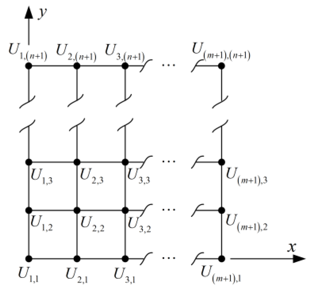
Figure 4. The quadrilateral ABCD. Arrangement of (n +1) × (m +1) nodal points in a 2D patch.

5.1. Lagrange polynomials

Let a 2D patch, on the plane

O x y

, interpolated through a net of

(m + 1)

vertical and

(n + 1)

horizontal lines (also called stations). The vertical lines intersect the

x

-axis at the nodal points

\{x_{1}, x_{2}, \dots, x_{m + 1}\}

, whereas the horizontal lines intersect the

y

-axis at the nodal points

\{y_{1}, y_{2}, \dots, y_{n + 1}\}

, as shown in Figure 4. In general, the

i

-th vertical line (which passes through the point

x = x_{i}

) will intersect the

j

-th horizontal line (which passes through the point

y = y_{j}

) at the point

P_{i, j} (x_{i, j}, y_{i, j}) = (x_{i}, y_{j})

, which is associated to a value

U_{i, j}

. In other words, the first index “i” is associated to the

x

-direction, while the second index “j” is associated to the

y

-direction.

When the variable is bivariate,

u (x, y)

, Equation (22) is replaced by the tensor product:

u (x, y) = \sum_{j = 1}^{n + 1} \sum_{i = 1}^{m + 1} L_{i} (x) L_{j} (y) U_{i, j},

(31)

where

U_{i, j}

are the nodal values associated to the Lagrange basis functions

L_{i} (x)

and

L_{j} (y)

. In our formulation, the totality of nodal points is stored into a matrix

U

of size

(m + 1) \times (n + 1)

, arranged in

(m + 1)

matrix rows and

(n + 1)

matrix columns, as follows:

U = [\begin{matrix} U_{1, 1} & \dots & U_{1, (n + 1)} \\ ⋮ & ⋱ & ⋮ \\ U_{(m + 1), 1} & \dots & U_{(m + 1), (n + 1)} \end{matrix}]

(32)

In other words, the

j

-th column of matrix U in Eq. (12) represents the

j

-th row in the spatial arrangement of Figure 4, measured from bottom. Similarly, the

i

-th row of matrix U corresponds to the

i

-th column of Figure 4, measured from left.

Given the abovementioned net of nodal points stored in

U

, the tensor product in this patch is written in the form:

u (x, y) = L_{x}^{T} \cdot U \cdot L_{y},

(33)

with

L_{x} = {[\begin{matrix} L_{1} (x) & \dots & L_{m + 1} (x) \end{matrix}]}^{T}

(34a)

and

L_{y} = {[\begin{matrix} L_{1} (y) & \dots & L_{n + 1} (y) \end{matrix}]}^{T}

(34b)

5.2 Bernstein polynomials

Based on the matrix form of tensor-product Lagrange basis polynomials (Equation (33)), it is easy to show that a similar tensor-product Bernstein basis polynomials is derived as well.

By substituting Equation (29) into Equation (33), we receive:

\begin{array}{l} u (x, y) & = {(T_{x} B_{x})}^{T} \cdot U \cdot (T_{y} B_{y}) \\ = B_{x}^{T} \cdot (T_{x}^{T} U T_{y}) \cdot B_{y} \end{array}

(35)

By introducing the matrix:

A = T_{x}^{T} U T_{y},

(36)

Equation (15) is written as:

u (x, y) = B_{x}^{T} \cdot A \cdot B_{y}

(37)

Since Equation (37) has the same form with Equation (33) which is a tensor product of Lagrange polynomials, it is obvious that the bivariate function can be written as a tensor product of Bernstein polynomials

u (x, y) = \sum_{j = 1}^{n + 1} \sum_{i = 1}^{m + 1} B_{i, m} (x) B_{j, n} (y) α_{i j},

(38)

associated to arbitrary coefficients

α_{i, j}

which form a matrix A given by Equation (16).

In other words, the non-rational tensor-product of Bernstein-Bézier basis polynomials is only a linear transformation of the tensor-product of Lagrange basis polynomials.

5.3 . B-splines

Since the univariate B-spline is a generalization of the Lagrange and Bernstein polynomials, simply by inserting a piecewise character in the interpolation, it is reasonable that bivariate interpolation may be carried by the analogy of Equation (38), that is by the formula:

u (x, y) = \sum_{j = 1}^{n + 1} \sum_{i = 1}^{m + 1} N_{i, p} (x) N_{j, q} (y) α_{i j},

(40)

where p and q are the polynomial degrees in the x- and y-direction, respectively.

5.4. NURBS approximation

By the analogy of Equation (40), the interpolation in a curvilinear NURBS patch is given by the formula:

u (x, y) = \sum_{j = 1}^{n + 1} \sum_{i = 1}^{m + 1} R_{i j, p q} (x, y) α_{i j},

(43)

where

R_{i j, p q} (x, y)

is the bivariate NURBS basis function:

R_{i j, p q} (x, y) = \frac{w_{i j} N_{i, p} (x) N_{j, q} (y)}{\sum_{j = 1}^{n + 1} \sum_{i = 1}^{m + 1} w_{i j} N_{i, p} (x) N_{j, q} (y)},

(44)

The latter is a true tensor-product only when the weight

w_{i j} = w_{i} w_{j}

, otherwise the denominator of Equation (44) includes the sum of all the

(m + 1) \times (n + 1)

terms.

6. The proposed Conjecture

Considering the material which was systematically presented and discussed in the previous sections, this paper makes the innovative step beyond the state-of-the-art and tests the hypothesis (or conjecture) that:

CONJECTURE: In the transfinite interpolation, the blending functions may be any complete and linear independent set provided the Partition of Unity Property is preserved.

It is worthy to mention that the original transfinite interpolation formula (by Coons and later by Gordon) is heuristic, and thus cannot be mathematically sustained (in absolute sense). According to Ref. [7](p. 114), ”. . . it is guided by experience, geometric intuition and analysis, and is accomplished with the aid of computer graphics, i.e. actual visual inspection”.

Since the original source is heuristic, the novel idea is obviously heuristic as well.

The proposed conjecture was progressively established in author’s mind, step-by-step, as follows. In the beginning, it was found that it is sufficient to ‘mechanically’ replace all the Lagrange polynomials involved in the transfinite interpolation of a curvilinear patch (i.e. the blending and the trial functions) by Bernstein-Bézier polynomials of the same degree. In this way, it was made possible to determine the weights associated with the control points so that the patch may accurately represent a circular or a spherical part [17]. The amazing issue related to the previously mentioned mechanical replacement, is that the produced shape functions are fully symmetrical with respect to the geometry of the patch (see, [17]), and this was precisely the cause of the inspiration for the present conjecture.

The argumentation in favour of the above conjecture continues below.

6.1. Bernstein tensor-product elements

In this context, first let us consider the tensor product Bernstein elements (e.g. Fig. 3a). Obviously, here the assumption that blending and trial functions are both Bernstein polynomials denoted by the symbol

B

(E_{i} = B_{i}, {\tilde{B}}_{j} = B_{j})

, leads to three equal projectors in the transfinite interpolation, i.e.

P_{ξ} = P_{η} = P_{ξ η}

, and therefore the Boolean sum becomes

P_{ξ} + P_{η} - P_{ξ η} \equiv P_{ξ η}

(compare with Theorem-1). Since the assumption of Bernstein polynomial as blending functions lead to the anticipated tensor-product, the proposed Conjecture is verified. As an example, the case of uniform control points in the tensor-product Bernstein-Bézier patch is shown in Fig. 3a. We recall that, according to section 2.2, the uniform tensor-product of Bernstein polynomials of fourth degree (shown in Fig. 3a) is equivalent to the unform tensor-product of Lagrange polynomials of the same degree (shown in Fig. 2a).

6.2. B-spline tensor-product elements

Let us now consider a B-spline patch of degree p. Again, the assumption of both blending and trail functions as univariate B-splines, leads to a Boolean sum equal to the anticipated tensor-product of B-splines. Therefore, again, our hypothesis is still reliable.

6.3. NURBS tensor-product elements

Considering now a NURBS patch with weights

w_{i j} = w_{i} w_{j}

, and repeating the same procedure, the Boolean sum leads to a tensor-product NURBS patch.

6.4. Overall evidence for tensor-product elements

Therefore, summarizing the above findings and the review of this section, we report:

Regarding the tensor-product, for any of the four kinds of trial functions (i.e. Lagrange, Bernstein, B-splines, NURBS), this is the outcome of transfinite interpolation in which the blending functions are identical with the trial functions.
Piecewise-linear blending functions are admissible, since when combined with piecewise-linear trial functions lead to an assembly of conventional bilinear finite elements (see, Ref. [26](p.956)).
Pure transfinite elements, with nodal points distributed along stations (i.e. different than tensor-product arrangement), gave the same result when the Lagrange polynomials were mechanically replaced by Bernstein polynomials. This is equivalent to considering Bernstein polynomial for both blending and interpolating purposes.
All the above successful cases are characterized by completeness, linear independence and all of them have the Partition of Unity Property.

6.5. Applications

6.5.1. The 21-node transfinite element

Regarding the 21-node transfinite element (Figure 2a), since there are three stations per direction (ends and middle), the blending functions may be Lagrange polynomials of degree 2, whereas the trial functions may be Lagrange polynomials of degree 4 (because there are five nodes along each edge and any internal station), as shown in Figure 5a.

Implementing the conjecture of the present paper, if we assume that the blending functions are Bernstein polynomials of degree 2 whereas the trial functions are Bernstein polynomials of degree 4, the final closed-form expression of the global shape functions is merely the replacement of the Lagrange by the Bernstein polynomials, as shown in Figure 5b. The latter has been previously performed by intuition in Ref. [17], but the present paper generalizes this idea and promotes the implementation of other trial functions apart from Bernstein polynomials as well (e.g., B-splines, NURBS).

In addition to that, we can preserve the blending function as a Bernstein polynomial of degree 2, whereas the trial function must be consistent to the five nodal points along each station. The latter can be accomplished by five control points which are consistent with either of the following choices for the trial functions:

A Bernstein polynomial of degree p = 4 and the obvious knot vector U = [0,0,0,0,0, 1,1,1,1,1]. This choice was already mentioned above and is shown in Figure 5b.
A cubic B-spline (p = 3) with knot vector U = [0,0,0,0, 1/2, 1,1,1,1], shown in Figure 5c.
A quadratic B-spline (p = 2) with knot vector U = [0,0,0, 1/3, 2/3, 1,1,1], shown in Figure 5d.

To give an idea about the performance of these elements, at the 21 nodes of Figure 2a we collocate the function

f (x, y) = e^{x} \cos (π y)

, and then interpolate in the interior of the element using the 21 global shape functions. The results are shown in Table 1, where one may observe that Lagrange and Bernstein polynomials of the same degree led to the same result. The replacement of the fully polynomial trial functions with B-splines decreased accuracy but not that much.

6.5.2. The 113-node transfinite element

The concern with the 113-node element (Figure 2d), is whether the involved Lagrange and Bernstein polynomials of higher degree (p_x = 16, p_y = 12) lead to numerical oscillations. Actually, one may observe the high values in Figure 6(a) when Lagrange polynomals are used.

This shortcoming is overcome by the proposed novel procedure, according to which we can consider that the blending functions be B-splines of degree (say)

p = 3

, in conjunction with the proper knot vector which produces so many control points as the number of nodal points per station.

In contrast, Figure 6(b) shows that when both blending and trial functions are chosen as Bernstein polynomials, the positive high values of the basis functions fully disappear, but small negative values still remain.

One would expect that the non-negative Bernstein polynomials would also lead to non-negative basis functions, which of course is true when only tensor products are involved. To explain this issue, below we isolate the first two out of the 113 basis functions:

\begin{array}{l} ϕ_{1} (ξ, η) = E_{0} (ξ) L_{0}^{(12)} (η) + L_{0}^{(16)} (ξ) E_{0} (η) - E_{0} (ξ) E_{0} (η), \\ ϕ_{2} (ξ, η) = L_{\frac{1}{16}}^{(16)} (ξ) E_{0} (η) . \end{array}

(45a)

The first equality in the Lagrange-polynomial based Equation (45a) is associated to the node ‘1’ and corresponds to a typical intersection between two stations. The second equality is associated to node ‘2’ and refers to a typical intermediate node of a station. Based on the number of stations per direction, the blending functions

E_{0} (ξ)

and

E_{0} (η)

are Lagrange polynomials of degree 4 and 3, respectively. Moreover,

L_{i}^{(16)} (ξ)

are Lagrange polynomials of degree 16 for interpolating along the horizontal stations, whereas

L_{j}^{(12)} (η)

are Lagrange polynomials of degree 12 for interpolating along the vertical stations. Since Lagrange polynomials take positive and negative values, the shape of Figure 6(a) is fully justified.

Furthermore, even if the Lagrange polynomials are replaced by the non-negative Bernstein polynomials as follows:

E_{0} (ξ) \to B_{0, 4} (ξ)

E_{0} (η) \to B_{0, 3} (η)

, etc,

L_{0}^{(16)} (ξ) \to B_{0, 16} (ξ)

, etc, the basis functions

ψ_{1} (ξ, η), ψ_{2} (ξ, η)

and the similars may obviously obtain negative values:

\begin{array}{l} ψ_{1} (ξ, η) = B_{0, 4} (ξ) B_{0, 12} (η) + B_{0, 16} (ξ) B_{0, 3} (η) - B_{0, 4} (ξ) B_{0, 3} (η), \\ ψ_{2} (ξ, η) = B_{1, 16} (ξ) B_{0, 3} (η) . \end{array}

(45b)

To evaluate the quality of the approximation using transfinite interpolation, in both cases (Lagrange-Lagrange and Bernstein-Bernstein), after collocating the function

f (x, y) = e^{x} \cos (π y)

at the 113 nodal points, Table 2 shows that the L2-error norm equals to only (1.2326 × 10^-5) %. Since the maximum polynomial degree involved in the L2-norm is 2 × 16 = 32, a 17 × 17 Gaussian scheme was imposed for the entire patch.

In the case of the combination of blending functions using either Lgrange or Bernstein polynomials in conjunction with cubic B-splines based on 14 and 10 uniform knot spans in x- and y-directions (thus producing 17 and 13 control points), respectively, the basis functions are shown in Figure 6(c). In the latter case, the domain was divided into 14 × 10 uniform cells (elements), and on each element a 4 × 4 Gaussian scheme was imlemented. The L2-error norm was found equal to 0.0013%.

7. Unstructured transfinite elements

Now we leave the structured stencils shown in Figure 2 (developed at General Motors Research Laboratories), and deal with patches in which the nodes (or the control points) do not lie along isolines only, as was the case discussed in section 6. There are many gradations of this group, at least as follows:

The internal nodes form a tensor product, but are not consistent with the boundary nodes (neither the position nor the quantity);
The internal nodes have been produced after a number of subdivisions (see Section 8);
The internal nodes are arranged like the well-known T-mesh (see Section 9).

All the above three categories may be tackled using univariate blending and trial functions which may be (i) Lagrange polynomials, (ii) Bernstein polynomials, (iii) B-splines, and (iv) NURBS (when curvilinear).

The treatment of all these cases may be faced with a well-programmed computer program, but for the sake of clariness, below we present typical cases separately.

7.1. Tensor-product-like 25-node element

To this purpose, let us consider the 25-node element shown in Figure 3b, which is a distrorted tensor-product of which some boundary nodes have been shifted from their uniform position. Therein, one may observe 25 nodes (16 on the boundary in form of black circles, and 9 inner nodes denoted by red-coloured circles). The characteristic of this element is that some of the normal projections of the inner nodes on the boundary are shifted with respect to the boundary positions. To depict this deviation, these projections (called artificial points) are denoted by smaller auxiliary numbers in green (nodes 26,…,35), and green-coloured crosses (×).

The first question to answer below is, whether the Lagrange-polynomial and the Bernstein-polynomial based numerical solution is the same, and how it is performed and justified.

7.1.1. Lagrange-polynomial based elements

The number of layers of internal nodes per direction defines the degree of the blending functions, which in principle are Lagrange polynomials. Applying the transfinite (Gordon) interpolation to the assemblage of the internal nodes and the artificial points, after all these artificial nodes are interpolated in terms of the actual nodes along the corresponding edge, we eventually derive two types of global shape functions as follows:

Those along the boundary, depending on both the trial functions and the associated blending function in the normal direction. By construction, they vanish at all the boundary nodes (except for one) and vanish at all the internal nodes.
Those global shape functions, associated with the inner nodes. They are the well-known classical tensor product Lagrangian polynomials (i.e., the blending functions).

For the distorted setup of nodes shown in Figure 3b, the closed-form expressions of the Lagrange-polynomial based global shape functions have been derived in Appendix B and are illustrated in Figure 7(a).

7.1.2. Bernstein-polynomial based elements

While the Lagrange-based global basis functions depend on whether the associated nodal point is at the corner (and then is an actual Boolean sum of blending and trial functions) or is intermediate on the boundary, Bernstein polynomials operate in a slightly different way as is discussed below.

For the distorted setup of twenty-five nodes shown in Figure 3b, the stations to which the Bernstein polynomials refer are uniformly distributed, and thus blending and trial sets coincide one another. Consequently, in Equation (B.5) (of Appendix B) the Lagrange polynomials must be replaced by Bernstein polynomials of the same degree, and the result is illustrated in Figure 7(b). Obviously, this means that for all the internal nodes and the intermediate boundary nodes, the global basis functions will be tensor-product Bernstein polynomials. Furthermore, if the same replacement is performed for a corner node (say the bottom left No. 1), the result will be again a perfect tensor product:

\begin{array}{l} {[N_{1} (ξ, η)]}_{Bernstein} & = B_{0, 4} (ξ) B_{0, 4} (η) + B_{0, 4} (η) B_{0, 4} (ξ) - B_{0, 4} (ξ) B_{0, 4} (η) \\ = B_{0, 4} (ξ) B_{0, 4} (η) . \end{array}

(46)

In other words, the analogue of a distorted tensor-product Lagrangian transfinite element is an ideal tensor-product Bernstein polynomials (with symmetrically placed control points), and this is possible because any deviation from symmetry is absorbed by the generalized coefficients α.

Interestingly, setting the values of the function

u (x, y) = e^{x} \cos (π y)

at the same 25 non-uniform places, in both formulations (Lagrange, Bernstein) the L2-error norm within the square domain was found equal to L2 = 0.6361%.

7.2. Tensor-product-like 27-node element

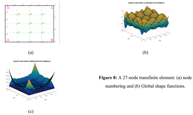
Another instructive example of a generalized 27-node transfinite element, a little more complex than that described above, is shown in Figure 8a. One may observe that the opposite edges are divided into a uniform but different number of subdivisions to one another.

The three stations of internal nodes parallel to the horizontal axis depict blending functions

E_{i} (ξ)

of fourth degree in

ξ

(with

i = 1, \dots, 5

). Similarly, the three stations of internal nodes parallel to the vertical axis (thus five stations, in total, including the edges AD and BC) depict blending functions

E_{j} (η)

again of fourth degree in

η

Regarding the trial functions, the edge AB requires a polynomial of fourth degree (i.e.,

L_{i}^{(4) A B} (ξ)

with

i = 1, \dots, 5

), the edge BC of third degree (i.e.,

L_{j}^{(3) B C} (η)

with

j = 1, \dots, 4

), the edge DC of sixth degree, whereas the edge AD needs a polynomial of fifth degree.

As usual, we distinguish three categories of nodes, i.e. those at corners, those at intermediate boundary nodes, and finally those in the interior. The totality of the basis functions is shown in Equation (47), where

L

represent the Lagrange polynomials performing as trial functions.

When working with Lagrange polynomials for blending and trial functions, not only the degree of the polynomial but also the location of the involved nodes plays a certain role. We recall that in the previous example of 25-node element (section 7.1), although the inner nodes were uniformly distributed, the nonuniform location of the nodes 2, 3, and 4 was introduced in the set of the five Lagrange polynomials along the bottom edge AB. The same holds true in the 27-node element under consideration:

\begin{array}{l} B o u n d a r y n o d e s : \\ N_{1} (ξ, η) = E_{1} (ξ) L_{1}^{A D} (η) + E_{1} (η) L_{1}^{A B} (ξ) - E_{1} (ξ) E_{1} (η), \\ N_{2} (ξ, η) = E_{1} (η) L_{2}^{A B} (ξ), \\ N_{3} (ξ, η) = E_{1} (η) L_{3}^{A B} (ξ), \\ N_{4} (ξ, η) = E_{1} (η) L_{4}^{A B} (ξ), \\ N_{5} (ξ, η) = E_{5} (ξ) L_{1}^{B C} (η) + E_{1} (η) L_{5}^{A B} (ξ) - E_{5} (ξ) E_{1} (η), \\ N_{6} (ξ, η) = E_{5} (ξ) L_{2}^{B C} (η), \\ N_{7} (ξ, η) = E_{5} (ξ) L_{3}^{B C} (η), \\ N_{8} (ξ, η) = E_{5} (ξ) L_{4}^{B C} (η) + E_{5} (η) L_{7}^{D C} (ξ) - E_{5} (ξ) E_{5} (η), \\ N_{9} (ξ, η) = E_{5} (η) L_{6}^{D C} (ξ), \\ N_{10} (ξ, η) = E_{5} (η) L_{5}^{D C} (ξ), \\ N_{11} (ξ, η) = E_{5} (η) L_{4}^{D C} (ξ), \\ N_{12} (ξ, η) = E_{5} (η) L_{3}^{D C} (ξ), \\ N_{13} (ξ, η) = E_{5} (η) L_{2}^{D C} (ξ), \\ N_{14} (ξ, η) = E_{1} (ξ) L_{6}^{A D} (η) + E_{5} (η) L_{1}^{D C} (ξ) - E_{1} (ξ) E_{5} (η), \\ N_{15} (ξ, η) = E_{1} (ξ) L_{5}^{A D} (η), \\ N_{16} (ξ, η) = E_{1} (ξ) L_{4}^{A D} (η), \\ N_{17} (ξ, η) = E_{1} (ξ) L_{3}^{A D} (η), \\ N_{18} (ξ, η) = E_{1} (ξ) L_{2}^{A D} (η), \\ I n n e r n o d e s : \\ N_{19} (ξ, η) = E_{2} (ξ) E_{2} (η), \\ N_{20} (ξ, η) = E_{3} (ξ) E_{2} (η), \\ N_{21} (ξ, η) = E_{4} (ξ) E_{2} (η), \\ N_{22} (ξ, η) = E_{2} (ξ) E_{3} (η), \\ N_{23} (ξ, η) = E_{3} (ξ) E_{3} (η), \\ N_{24} (ξ, η) = E_{4} (ξ) E_{3} (η), \\ N_{25} (ξ, η) = E_{2} (ξ) E_{4} (η), \\ N_{26} (ξ, η) = E_{3} (ξ) E_{4} (η), \\ N_{27} (ξ, η) = E_{4} (ξ) E_{4} (η) . \end{array}

(47)

In contrast, when working with Bernstein polynomials, only the polynomial degrees are of interest, since the nodal points do not contribute to the formulation of the basis functions.

Focusing on Figure 8a, the blending functions are polynomials of degree four, either uniform Lagrange or Bernstein, accordingly.

Moreover, in both formulations (i.e., Lagrange and Bernstein), the corners nodes 1 and 5 eventually appear only in the

P_{ξ}

projection, whereas the rest corner nodes 8 and 14 are influenced by all the three projections.

The result shown in Figure 8b has been obtained using Lagrange polynomials as blending functions of fourth degree, and for the edges it is as follows: The edges AB (bottom), BC, CD and DA are interpolated by polynomials or degree 4, 3, 6, and 5, respectively.

Regarding the Bernstein formulation, the bivariate basis functions are given by replacing the Lagrange with Bernstein polynomials of the same degree in Equation (47) and are illustrated in Figure 8(c).

It is also noted that, in both formulations, the determinant of the Jacobian takes everywhere its accurate value, and the partition of unity holds everywhere.

Now, setting the values of the function

u (x, y) = e^{x} \cos (π y)

at the 27 uniform places on the boundary and the interior (nodes 1 to 27), the 27 coefficients α of the distrorted tensor-product Bernstein-Bézier element were calculated. Based on these two sets of 27 values separately (U or α values), a small difference was found for the L2-error norm within the square domain (Lagrange formulation according to Equation (47): L2 = 0.6408%, Bernstein formulation: L2 = 0.6154%).

8. Mesh Refinement

There are many engineering problems in which the exact solution varies rapidly at a certain point of the domain. Due to this high gradient, it becomes necessary to refine the mesh at this point of the domain, but then the problem of hanging nodes appears.

A simple method to overcome this problem is to subdivide the initial patch ABCD, using progressively one-fourth of the previous subdomain closest to the ‘singularity’ at the corner D, as shown in Figure 9. One may observe the hanging nodes 5 and 10 after the first refinement, as well as 15 and 18 after the second refinement. Below, we will see that in the transfinite formulation they do not constitute a difficulty to deal with.

Therefore, starting from the classical quadratic element shown in Figure 9a, we subdivide the upper left fourth, as shown in Figure 9b. In this case, we have four vertical stations at

ξ = 0, \frac{1}{4}, \frac{1}{2}, 1

in the horizontal and

η = 0, \frac{1}{2}, \frac{3}{4}, 1

in the vertical direction.

As was shown in the previous sections, we are flexible in choosing the blending and trial functions. Below we present the global shape functions when Lagrange polynomials have been implemented everywhere. Then, the blending functions are Lagrange polynomials of third degree but are based on non-uniform nodes (not the same in the two directions, and thus the subscripts denote the position of each associated station):

x-direction:

E_{0} (ξ), E_{\frac{1}{4}} (ξ), E_{\frac{2}{4}} (ξ), E_{1} (ξ)

y-direction:

E_{0} (η), E_{\frac{2}{4}} (η), E_{\frac{3}{4}} (η), E_{1} (η)

Regarding the trial functions, we distinguish three sets of Lagrange polynomials, as follows:

- Those along the boundary stations AB and BC, which are uniform quadratic polynomials

(p = 2)

L_{0}^{(2)} (s) = (2 s - 1) (s - 1)

L_{\frac{1}{2}}^{(2)} (s) = 4 s (1 - s)

, and

L_{1}^{(2)} (s) = s (2 s - 1)

, where

s

denotes either of

ξ

η

- Those along the horizontal stations 4-5-6-7 and 11-12-13-14, which are non-uniform Lagrange polynomials, identical with the blending functions toward the

ξ

-axis:

L_{0}^{(3)} (ξ) = E_{0} (ξ),

L_{\frac{1}{4}}^{(3)} (ξ) = E_{\frac{1}{4}} (ξ),

L_{\frac{2}{4}}^{(3)} (ξ) = E_{\frac{2}{4}} (ξ),

and

L_{1}^{(3)} (ξ) = E_{1} (ξ)

- Those along the vertical stations 1-4-8-11 and 2-6-10-13, which are identical with the blending functions toward the

η

-axis:

L_{0}^{(3)} (η) = E_{0} (η),

L_{\frac{2}{4}}^{(3)} (η) = E_{\frac{2}{4}} (η),

L_{\frac{3}{4}}^{(3)} (η) = E_{\frac{3}{4}} (η),

and

L_{1}^{(3)} (η) = E_{1} (η)

Based on the above three functional sets of trial functions, the application of the Boolean sum in conjunction with artificial nodes which are the intersections of the line 9-5 with 1-2 and the line 9-10 with 7-14, leads to the following global shape functions for the entire patch (for details, see Appendix C):

\begin{array}{l} N_{1} (ξ, η) = E_{0} (ξ) L_{0}^{(3)} (η) + E_{0} (η) L_{0}^{(2)} (ξ) - E_{0} (ξ) E_{0} (η), \\ N_{2} (ξ, η) = E_{\frac{2}{4}} (ξ) L_{0}^{(3)} (η) + E_{0} (η) L_{\frac{1}{2}}^{(2)} (ξ) - E_{\frac{2}{4}} (ξ) E_{0} (η), \\ N_{3} (ξ, η) = E_{1} (ξ) L_{0}^{(2)} (η) + E_{0} (η) L_{1}^{(2)} (ξ) - E_{1} (ξ) E_{0} (η), \\ N_{4} (ξ, η) = E_{0} (ξ) L_{\frac{2}{4}}^{(3)} (η) + E_{\frac{2}{4}} (η) L_{0}^{(3)} (ξ) - E_{0} (ξ) E_{\frac{2}{4}} (η), \\ N_{5} (ξ, η) = E_{\frac{1}{4}} (ξ) L_{\frac{2}{4}}^{(3)} (η) + E_{\frac{2}{4}} (η) L_{\frac{1}{4}}^{(3)} (ξ) - E_{\frac{1}{4}} (ξ) E_{\frac{2}{4}} (η), \\ N_{6} (ξ, η) = E_{\frac{2}{4}} (ξ) L_{\frac{2}{4}}^{(3)} (η) + E_{\frac{2}{4}} (η) L_{\frac{2}{4}}^{(3)} (ξ) - E_{\frac{2}{4}} (ξ) E_{\frac{2}{4}} (η), \\ N_{7} (ξ, η) = E_{1} (ξ) L_{\frac{1}{2}}^{(2)} (η) + E_{\frac{2}{4}} (η) L_{1}^{(3)} (ξ) - E_{1} (ξ) E_{\frac{2}{4}} (η), \\ N_{8} (ξ, η) = E_{0} (ξ) L_{\frac{3}{4}}^{(3)} (η) + E_{\frac{3}{4}} (η) L_{0}^{(3)} (ξ) - E_{0} (ξ) E_{\frac{3}{4}} (η), \\ N_{9} (ξ, η) = E_{\frac{1}{4}} (ξ) L_{\frac{3}{4}}^{(3)} (η) + E_{\frac{3}{4}} (η) L_{\frac{1}{4}}^{(3)} (ξ) - E_{\frac{1}{4}} (ξ) E_{\frac{3}{4}} (η), \\ N_{10} (ξ, η) = E_{\frac{2}{4}} (ξ) L_{\frac{3}{4}}^{(3)} (η) + E_{\frac{3}{4}} (η) L_{\frac{2}{4}}^{(3)} (ξ) - E_{\frac{2}{4}} (ξ) E_{\frac{3}{4}} (η), \\ N_{11} (ξ, η) = E_{0} (ξ) L_{1}^{(3)} (η) + E_{1} (η) L_{0}^{(3)} (ξ) - E_{0} (ξ) E_{1} (η), \\ N_{12} (ξ, η) = E_{\frac{1}{4}} (ξ) L_{1}^{(3)} (η) + E_{1} (η) L_{\frac{1}{4}}^{(3)} (ξ) - E_{\frac{1}{4}} (ξ) E_{1} (η), \\ N_{13} (ξ, η) = E_{\frac{2}{4}} (ξ) L_{1}^{(3)} (η) + E_{1} (η) L_{\frac{2}{4}}^{(3)} (ξ) - E_{\frac{2}{4}} (ξ) E_{1} (η), \\ N_{14} (ξ, η) = E_{1} (ξ) L_{1}^{(2)} (η) + E_{1} (η) L_{1}^{(3)} (ξ) - E_{1} (ξ) E_{1} (η) . \end{array}

(48)

The shape functions of Equation (48) are illustrated in Figure 10a, whereas after replacing the Lagrange with Bernstein polynomials, the updated basis functions are shown in Figure 10b.

Considering the almost singular function

u (x, y) = 1 / \ln (r + 0.1)

, in which the position

r

is measured from the top left corner D (node 11) of Figure 9, for both formulations (Lagrange and Bernstein polynomials), the 9-node element gave L2-error norm equal 10.7304%, whereas the 14-node decreased to 7.6496%.

Moreover, following the same procedure as above, the 19-node element which is shown in Figure 9(c), can be treated through the global basis functions:

\begin{array}{l} N_{1} (ξ, η) = E_{0} (ξ) L_{0}^{(4)} (η) + E_{0} (η) L_{0}^{(2)} (ξ) - E_{0} (ξ) E_{0} (η), \\ N_{2} (ξ, η) = E_{\frac{4}{8}} (ξ) L_{0}^{(3)} (η) + E_{0} (η) L_{\frac{1}{2}}^{(2)} (ξ) - E_{\frac{4}{8}} (ξ) E_{0} (η), \\ N_{3} (ξ, η) = E_{1} (ξ) L_{0}^{(2)} (η) + E_{0} (η) L_{1}^{(2)} (ξ) - E_{1} (ξ) E_{0} (η), \\ N_{4} (ξ, η) = E_{0} (ξ) L_{\frac{4}{8}}^{(4)} (η) + E_{\frac{4}{8}} (η) L_{0}^{(3)} (ξ) - E_{0} (ξ) E_{\frac{4}{8}} (η), \\ N_{5} (ξ, η) = E_{\frac{2}{8}} (ξ) L_{\frac{4}{8}}^{(4)} (η) + E_{\frac{4}{8}} (η) L_{\frac{1}{4}}^{(3)} (ξ) - E_{\frac{2}{8}} (ξ) E_{\frac{4}{8}} (η), \\ N_{6} (ξ, η) = E_{\frac{4}{8}} (ξ) L_{\frac{4}{8}}^{(3)} (η) + E_{\frac{4}{8}} (η) L_{\frac{2}{4}}^{(3)} (ξ) - E_{\frac{4}{8}} (ξ) E_{\frac{4}{8}} (η), \\ N_{7} (ξ, η) = E_{1} (ξ) L_{\frac{1}{2}}^{(2)} (η) + E_{\frac{4}{8}} (η) L_{1}^{(3)} (ξ) - E_{1} (ξ) E_{\frac{4}{8}} (η), \\ N_{8} (ξ, η) = E_{0} (ξ) L_{\frac{6}{8}}^{(4)} (η) + E_{\frac{6}{8}} (η) L_{0}^{(4)} (ξ) - E_{0} (ξ) E_{\frac{6}{8}} (η), \\ N_{9} (ξ, η) = E_{\frac{2}{8}} (ξ) L_{\frac{6}{8}}^{(4)} (η) + E_{\frac{6}{8}} (η) L_{\frac{2}{8}}^{(4)} (ξ) - E_{\frac{2}{8}} (ξ) E_{\frac{6}{8}} (η), \\ N_{10} (ξ, η) = E_{\frac{4}{8}} (ξ) L_{\frac{6}{8}}^{(3)} (η) + E_{\frac{6}{8}} (η) L_{\frac{4}{8}}^{(4)} (ξ) - E_{\frac{4}{8}} (ξ) E_{\frac{6}{8}} (η), \\ N_{11} (ξ, η) = E_{0} (ξ) L_{1}^{(4)} (η) + E_{1} (η) L_{0}^{(4)} (ξ) - E_{0} (ξ) E_{1} (η), \\ N_{12} (ξ, η) = E_{\frac{2}{8}} (ξ) L_{1}^{(4)} (η) + E_{1} (η) L_{\frac{2}{8}}^{(4)} (ξ) - E_{\frac{2}{8}} (ξ) E_{1} (η), \\ N_{13} (ξ, η) = E_{\frac{4}{8}} (ξ) L_{1}^{(3)} (η) + E_{1} (η) L_{\frac{4}{8}}^{(4)} (ξ) - E_{\frac{4}{8}} (ξ) E_{1} (η), \\ N_{14} (ξ, η) = E_{1} (ξ) L_{1}^{(2)} (η) + E_{1} (η) L_{1}^{(4)} (ξ) - E_{1} (ξ) E_{1} (η), \\ N_{15} (ξ, η) = E_{\frac{1}{8}} (ξ) L_{\frac{6}{8}}^{(4)} (η) + E_{\frac{6}{8}} (η) L_{\frac{1}{8}}^{(4)} (ξ) - E_{\frac{1}{8}} (ξ) E_{\frac{6}{8}} (η), \\ N_{16} (ξ, η) = E_{0} (ξ) L_{\frac{7}{8}}^{(4)} (η) + E_{\frac{7}{8}} (η) L_{0}^{(4)} (ξ) - E_{0} (ξ) E_{\frac{7}{8}} (η), \\ N_{17} (ξ, η) = E_{\frac{1}{8}} (ξ) L_{\frac{7}{8}}^{(4)} (η) + E_{\frac{7}{8}} (η) L_{\frac{1}{8}}^{(4)} (ξ) - E_{\frac{1}{8}} (ξ) E_{\frac{7}{8}} (η), \\ N_{18} (ξ, η) = E_{\frac{2}{8}} (ξ) L_{\frac{7}{8}}^{(4)} (η) + E_{\frac{7}{8}} (η) L_{\frac{2}{8}}^{(4)} (ξ) - E_{\frac{2}{8}} (ξ) E_{\frac{7}{8}} (η), \\ N_{19} (ξ, η) = E_{\frac{1}{8}} (ξ) L_{1}^{(4)} (η) + E_{1} (η) L_{\frac{1}{8}}^{(4)} (ξ) - E_{\frac{1}{8}} (ξ) E_{1} (η) . \end{array}

(49)

9. T-mesh like transfinite elements

The capability of transfinite elements to deal with mesh refinement is encouraging, and therefore it is important to check whether it can also treat unstructured domains in the form of T-mesh patches.

EXAMPLE-1: Let us consider the simple T-mesh shown in Figure 11. Below we test and compare several cases, such as polynomials (Lagrange and Bernstein) as well as cubic B-splines.

9.1. Lagrange and Bernstein polynomials

Regarding the application of the conventional transfinite interpolation, one may recognize in Figure 11(a) five vertical and another five horizontal uniform stations. Therefore, each of them will be polynomial of the fourth degree (

p_{x} = p_{y} = 4

To build the tree projectors, again we need to complete the tensor product by adding the two points (G and F) shown in Figure 11(b). Each of the three edges (BC, DC, and AD) contain five nodes and thus are represented by quartic polynomials, whereas the bottom edge AB includes only four nodes (1, 2 , 3, and 4). Clearly, the function U(ξ,0) along AB will be represented using a non-uniform Lagrange polynomial of degree three, and this affects the projector P_η. In contrast, the auxiliary point G (between 2 and 3) is involved in the interpolation of the function U(ξ = 1/2, η) which participates as a third additive term in the projector P_ξ.

The complete procedure will be given below, but the symmetry of the mesh in Figure 11 with respect to the y-axis dictates, in advance, that the transfinite interpolation degenerates to only the vertical projector P_η.

Actually, in more detail we have:

\begin{array}{l} P_{ξ} & = E_{0} (ξ) [L_{0}^{(4)} (η) U_{1} + L_{\frac{1}{4}}^{(4)} (η) U_{5} + L_{\frac{2}{4}}^{(4)} (η) U_{9} + L_{\frac{3}{4}}^{(4)} (η) U_{14} + L_{1}^{(4)} (η) U_{19}] \\ + E_{\frac{1}{4}} (ξ) [L_{0}^{(4)} (η) U_{2} + L_{\frac{1}{4}}^{(4)} (η) U_{6} + L_{\frac{2}{4}}^{(4)} (η) U_{10} + L_{\frac{3}{4}}^{(4)} (η) U_{15} + L_{1}^{(4)} (η) U_{20}] \\ + E_{\frac{2}{4}} (ξ) [L_{0}^{(4)} (η) U_{G} + L_{\frac{1}{4}}^{(4)} (η) U_{H} + L_{\frac{2}{4}}^{(4)} (η) U_{11} + L_{\frac{3}{4}}^{(4)} (η) U_{16} + L_{1}^{(4)} (η) U_{21}] \\ + E_{\frac{3}{4}} (ξ) [L_{0}^{(4)} (η) U_{3} + L_{\frac{1}{4}}^{(4)} (η) U_{7} + L_{\frac{2}{4}}^{(4)} (η) U_{12} + L_{\frac{3}{4}}^{(4)} (η) U_{17} + L_{1}^{(4)} (η) U_{22}] \\ + E_{1} (ξ) [L_{0}^{(4)} (η) U_{4} + L_{\frac{1}{4}}^{(4)} (η) U_{8} + L_{\frac{2}{4}}^{(4)} (η) U_{13} + L_{\frac{3}{4}}^{(4)} (η) U_{18} + L_{1}^{(4)} (η) U_{23}], \end{array}

(50)

also

\begin{array}{l} P_{η} & = E_{0} (η) {[L_{0}^{(3) A B} (ξ) U_{1} + L_{\frac{1}{4}}^{(3) A B} (ξ) U_{2} + L_{\frac{2}{4}}^{(3) A B} (ξ) U_{3} + L_{1}^{(3) A B} (ξ) U_{4}]}_{B C} \\ + E_{\frac{1}{4}} (η) [L_{0}^{(3) η = 1 / 4} (ξ) U_{5} + L_{\frac{1}{4}}^{(3) η = 1 / 4} (ξ) U_{6} + L_{\frac{2}{4}}^{(3) η = 1 / 4} (η) U_{7} + L_{1}^{(3) η = 1 / 4} (η) U_{8}] \\ + E_{\frac{2}{4}} (η) [L_{0}^{(4)} (η) U_{9} + L_{\frac{1}{4}}^{(4)} (η) U_{10} + L_{\frac{2}{4}}^{(4)} (η) U_{11} + L_{\frac{3}{4}}^{(4)} (η) U_{12} + L_{1}^{(4)} (η) U_{13}] \\ + E_{\frac{3}{4}} (η) [L_{0}^{(4)} (η) U_{14} + L_{\frac{1}{4}}^{(4)} (η) U_{15} + L_{\frac{2}{4}}^{(4)} (η) U_{16} + L_{\frac{3}{4}}^{(4)} (η) U_{17} + L_{1}^{(4)} (η) U_{18}] \\ + E_{1} (η) [L_{0}^{(4)} (η) U_{19} + L_{\frac{1}{4}}^{(4)} (η) U_{20} + L_{\frac{2}{4}}^{(4)} (η) U_{21} + L_{\frac{3}{4}}^{(4)} (η) U_{22} + L_{1}^{(4)} (η) U_{23}], \end{array}

(51)

whereas the tensor product is:

\begin{array}{l} P_{ξ η} & = E_{0} (ξ) E_{0} (η) U_{1} + E_{\frac{1}{4}} (ξ) E_{0} (η) U_{2} + E_{\frac{2}{4}} (ξ) E_{0} (η) U_{G} + E_{\frac{3}{4}} (ξ) E_{0} (η) U_{3} + E_{1} (ξ) E_{0} (η) U_{4} \\ + E_{0} (ξ) E_{\frac{1}{4}} (η) U_{5} + E_{\frac{1}{4}} (ξ) E_{\frac{1}{4}} (η) U_{6} + E_{\frac{2}{4}} (ξ) E_{\frac{1}{4}} (η) U_{H} + E_{\frac{3}{4}} (ξ) E_{\frac{1}{4}} (η) U_{7} + E_{1} (ξ) E_{\frac{1}{4}} (η) U_{8} \\ + E_{0} (ξ) E_{\frac{2}{4}} (η) U_{9} + E_{\frac{1}{4}} (ξ) E_{\frac{2}{4}} (η) U_{10} + E_{\frac{2}{4}} (ξ) E_{\frac{2}{4}} (η) U_{11} + E_{\frac{3}{4}} (ξ) E_{\frac{2}{4}} (η) U_{12} + E_{1} (ξ) E_{\frac{2}{4}} (η) U_{13} \\ + E_{0} (ξ) E_{\frac{3}{4}} (η) U_{14} + E_{\frac{1}{4}} (ξ) E_{\frac{3}{4}} (η) U_{15} + E_{\frac{2}{4}} (ξ) E_{\frac{3}{4}} (η) U_{16} + E_{\frac{3}{4}} (ξ) E_{\frac{3}{4}} (η) U_{17} + E_{1} (ξ) E_{\frac{3}{4}} (η) U_{18} \\ + E_{0} (ξ) E_{1} (η) U_{19} + E_{\frac{1}{4}} (ξ) E_{1} (η) U_{20} + E_{\frac{2}{4}} (ξ) E_{1} (η) U_{21} + E_{\frac{3}{4}} (ξ) E_{1} (η) U_{22} + E_{1} (ξ) E_{1} (η) U_{23} . \end{array}

(52)

Since the trial functions

L_{i}^{(4)} (η)

are identical with the blending functions, i.e.

L_{i}^{(4)} (η) = E_{i} (η)

, one may observe that in this example we have:

P_{ξ} = P_{ξ η},

(53)

whence

\begin{array}{l} U (ξ, η) & = P_{ξ} + P_{η} - P_{ξ η} \\ = P_{η} . \end{array}

(54)

The cancelation of the difference

(P_{ξ} - P_{ξ η})

also means the cancelation of the involved auxiliary variables (

U_{G}

and

U_{H}

). Eventually, the factors of the 23 nodal values

U_{i}, i = 1, \dots, 23

in Equation (49) denote the desired shape functions of the macroelement associated with the patch ABCD, which are illustrated in Figure 12(a) using either Lagrange polynomials. When the Lagrange polynomials are replaced by Bernstein ones, we receive the set of 23 basis functions shown in Figure 12(b).

The quality of the above obtained 23 shape functions is evaluated as follows. Setting the nodal values equal to the function

f (x, y) = e^{x} \cos (π y)

, then the L₂-norm was found equal to 0.4968% (in both Lagrange and Bernstein polynomials).

9.2. B-spline blending and trial functions

As an innovative step beyond state-of-the-art T-splines, we consider that the blending functions are B-splines and the same holds for the trial functions as well.

9.2.1 Example 9-1

In this context, the existence of five stations per direction (see Figure 11 and its analogue Figure 13) is consistent with a univariate B-spline formulation with five control points which span the entire domain [0,1]. This can be accomplished as follows:

Quadratic B-spline (p = 2) in conjunction with knot vector U = [0,0,0, 1/3,2/3, 1,1,1];
Cubic B-spline (p = 3) in conjunction with knot vector U = [0,0,0,0, 1/2, 1,1,1,1].

The results for the L2-error norm are shown in Table 3.

Clearly, cases 7 and 8 of Table 3 were obtained using the transfinite interpolation formula given by Equation (51), in which the Lagrange polynomials were replaced by B-splines. A question here arises whether the so produced basis functions are related to those that can be obtained through the conventional rule of T-splines. To answer this question, we form the arrays (each of size 23 × 5) which for each anchor provide the local knot vectors for the T-mesh shown in Figure 13 (

U_{ξ}

toward ξ-direction,

V_{η}

toward η-direction):

U_{ξ} = [\begin{matrix} 0 & 0 & 0 & 0 & 1 \\ 0 & 0 & 0 & 1 & 1 \\ 0 & 0 & 1 & 1 & 1 \\ 0 & 1 & 1 & 1 & 1 \\ 0 & 0 & 0 & 0 & 1 \\ 0 & 0 & 0 & 1 & 1 \\ 0 & 0 & 1 & 1 & 1 \\ 0 & 1 & 1 & 1 & 1 \\ 0 & 0 & 0 & 0 & 0 . 5 \\ 0 & 0 & 0 & 0 . 5 & 1 \\ 0 & 0 & 0 . 5 & 1 & 1 \\ 0 & 0 . 5 & 1 & 1 & 1 \\ 0 . 5 & 1 & 1 & 1 & 1 \\ 0 & 0 & 0 & 0 & 0 . 5 \\ 0 & 0 & 0 & 0 . 5 & 1 \\ 0 & 0 & 0 . 5 & 1 & 1 \\ 0 & 0 . 5 & 1 & 1 & 1 \\ 0 . 5 & 1 & 1 & 1 & 1 \\ 0 & 0 & 0 & 0 & 0 . 5 \\ 0 & 0 & 0 & 0 . 5 & 1 \\ 0 & 0 & 0 . 5 & 1 & 1 \\ 0 & 0 . 5 & 1 & 1 & 1 \\ 0 . 5 & 1 & 1 & 1 & 1 \end{matrix}], V_{η} = [\begin{matrix} 0 & 0 & 0 & 0 & 0 . 5 \\ 0 & 0 & 0 & 0 & 0 . 5 \\ 0 & 0 & 0 & 0 & 0 . 5 \\ 0 & 0 & 0 & 0 & 0 . 5 \\ 0 & 0 & 0 & 0 . 5 & 1 \\ 0 & 0 & 0 & 0 . 5 & 1 \\ 0 & 0 & 0 & 0 . 5 & 1 \\ 0 & 0 & 0 & 0 . 5 & 1 \\ 0 & 0 & 0 . 5 & 1 & 1 \\ 0 & 0 & 0 . 5 & 1 & 1 \\ 0 & 0 & 0 . 5 & 1 & 1 \\ 0 & 0 & 0 . 5 & 1 & 1 \\ 0 & 0 & 0 . 5 & 1 & 1 \\ 0 & 0 . 5 & 1 & 1 & 1 \\ 0 & 0 . 5 & 1 & 1 & 1 \\ 0 & 0 . 5 & 1 & 1 & 1 \\ 0 & 0 . 5 & 1 & 1 & 1 \\ 0 & 0 . 5 & 1 & 1 & 1 \\ 0 . 5 & 1 & 1 & 1 & 1 \\ 0 . 5 & 1 & 1 & 1 & 1 \\ 0 . 5 & 1 & 1 & 1 & 1 \\ 0 . 5 & 1 & 1 & 1 & 1 \\ 0 . 5 & 1 & 1 & 1 & 1 \end{matrix}]

(55)

One may observe in Figure 14 that the basis functions which were produced through transfinite interpolation using cubic B-splines for both blending and trial functions, are identical with those obtained using the classical T-spline formulation based on the local knot vectors given by Equation (55). Numerically, the differences were less than 10^-16.

EXAMPLE-2: Missing boundary knots

In Figure 15(a,b) we present a trivial case of 14 nodes where the nodal points G and F are missing to complete the tensor product. The four stations per direction suggest blending functions of degree three. The third vertical station measured from left requires the artificial points G and interpolation of third degree. Similarly, the third horizontal station measured from bottom requires the artificial point F and polynomial of third degree. Using Lagrange polynomials, the three projectors and their Boolean sum are given below.

\begin{array}{l} P_{ξ} & = E_{0} (ξ) [E_{0} (η) U_{1} + E_{\frac{1}{3}} (η) U_{4} + E_{\frac{2}{3}} (η) U_{8} + E_{1} (η) U_{11}] \\ + E_{\frac{1}{3}} (ξ) [E_{0} (η) U_{2} + E_{\frac{1}{3}} (η) U_{5} + E_{\frac{2}{3}} (η) U_{9} + E_{1} (η) U_{12}] \\ + E_{\frac{2}{3}} (ξ) [E_{0} (η) U_{G} + E_{\frac{1}{3}} (η) U_{6} + E_{\frac{2}{3}} (η) U_{10} + E_{1} (η) U_{13}] \\ + E_{1} (ξ) {[L_{0}^{(2) B C} (η) U_{3} + L_{\frac{1}{3}}^{(2) B C} (η) U_{7} + L_{1}^{(2) B C} (η) U_{14}]}_{B C}, \end{array}

(56)

also

\begin{array}{l} P_{η} & = E_{0} (η) {[L_{0}^{(2) A B} (ξ) U_{1} + L_{\frac{1}{3}}^{(2) A B} (ξ) U_{2} + L_{1}^{(2) A B} (ξ) U_{3}]}_{B C} \\ + E_{\frac{1}{3}} (η) [E_{0} (η) U_{4} + E_{\frac{1}{3}} (η) U_{5} + E_{\frac{2}{3}} (η) U_{6} + E_{1} (η) U_{7}] \\ + E_{\frac{2}{3}} (η) [E_{0} (η) U_{8} + E_{\frac{1}{3}} (η) U_{9} + E_{\frac{2}{3}} (η) U_{10} + E_{1} (η) U_{F}] \\ + E_{1} (η) [E_{0} (η) U_{11} + E_{\frac{1}{3}} (η) U_{12} + E_{\frac{2}{3}} (η) U_{13} + E_{1} (η) U_{14}], \end{array}

(57)

whereas the tensor product is:

\begin{array}{l} P_{ξ η} & = E_{0} (ξ) E_{0} (η) U_{1} + E_{\frac{1}{3}} (ξ) E_{0} (η) U_{2} + E_{\frac{2}{3}} (ξ) E_{0} (η) U_{G} + E_{1} (ξ) E_{0} (η) U_{3} \\ + E_{0} (ξ) E_{\frac{1}{3}} (η) U_{4} + E_{\frac{1}{3}} (ξ) E_{\frac{1}{3}} (η) U_{5} + E_{\frac{2}{3}} (ξ) E_{\frac{1}{3}} (η) U_{6} + E_{1} (ξ) E_{\frac{1}{3}} (η) U_{7} \\ + E_{0} (ξ) E_{\frac{2}{3}} (η) U_{8} + E_{\frac{1}{3}} (ξ) E_{\frac{2}{3}} (η) U_{9} + E_{\frac{2}{3}} (ξ) E_{\frac{2}{3}} (η) U_{10} + E_{1} (ξ) E_{\frac{2}{3}} (η) U_{F} \\ + E_{0} (ξ) E_{1} (η) U_{11} + E_{\frac{1}{3}} (ξ) E_{1} (η) U_{12} + E_{\frac{2}{3}} (ξ) E_{1} (η) U_{13} + E_{1} (ξ) E_{1} (η) U_{14} . \end{array}

(58)

One may observe that:

The interpolation along the right vertical edge BC is fully preserved using non-uniform polynomials of degree 2, and this justifies the subscript BC (boundary conditions) in the last square bracket of the projector $P_{ξ}$ (see Equation (56)).
The interpolation along the bottom edge AB is fully preserved using non-uniform polynomials of degree 2, and this justifies the subscript BC (boundary conditions) in the first square bracket of the projector $P_{η}$ (see Equation (57)).
The artificial values ( $U_{G}, U_{F}$ ) appear in the projectors $P_{ξ}$ and $P_{η}$ , respectively, whereas both of them appear in the tensor product $P_{ξ η}$ . As a result, they are eventually eliminated.
After performing the Boolean sum $P_{ξ} \otimes P_{η} = P_{ξ} + P_{η} - P_{ξ η}$ , the transfinite interpolation offers the following 14 global shape functions in the domain $[0, 1] \times [0, 1]$ :

$\begin{array}{l} U (ξ, η) = & [L_{0}^{(2) A B} (ξ) E_{0} (η)] \cdot U_{1} \\ + [L_{\frac{1}{3}}^{(2) A B} (ξ) E_{0} (η)] \cdot U_{2} \\ + [E_{1} (ξ) L_{0}^{(2) A B} (η) + L_{1}^{(2) A B} (ξ) E_{0} (η) - E_{1} (ξ) E_{0} (η)] \cdot U_{3} \\ + [E_{0} (ξ) E_{\frac{1}{3}} (η)] \cdot U_{4} \\ + [E_{\frac{1}{3}} (ξ) E_{\frac{1}{3}} (η)] \cdot U_{5} \\ + [E_{\frac{2}{3}} (ξ) E_{\frac{1}{3}} (η)] \cdot U_{6} \\ + [E_{1} (ξ) L_{\frac{1}{3}}^{(2) B C} (η)] \cdot U_{7} \\ + [E_{0} (ξ) E_{\frac{2}{3}} (η)] \cdot U_{8} \\ + [E_{\frac{1}{3}} (ξ) E_{\frac{2}{3}} (η)] \cdot U_{9} \\ + [E_{\frac{2}{3}} (ξ) E_{\frac{2}{3}} (η)] \cdot U_{10} \\ + [E_{0} (ξ) E_{1} (η)] \cdot U_{11} \\ + [E_{\frac{1}{3}} (ξ) E_{1} (η)] U_{12} \\ + [E_{\frac{2}{3}} (ξ) E_{1} (η)] \cdot U_{13} \\ + [E_{1} (ξ) L_{1}^{(2) B C} (η)] \cdot U_{14} \\ = \sum_{j = 1}^{14} ϕ_{j} (ξ, η) U_{j} . \end{array}$

(59)

The fourteen shape functions of Equation (59) are illustrated in Figure 16(a), and thus they obtain positive and negative values. Although at the nodes they take the value of unity, in between them they may exceed the unity.

Furthermore, if blending and trial functions are Bernstein polynomials of the same degree as the previously mentioned Lagrange polynomials, the form of Equation (59) is again derived, and the updated results are illustrated in Figure 16(b). One may recognize the Bernstein polynomials on the boundaries and may observe only positive values.

It is noted that in both cases, i.e. using either Lagrange of Bernstein polynomials, the partition of unity is fulfilled:

\sum_{j = 1}^{14} ϕ_{j} (ξ, η) = 1, \forall (ξ, η) \in {[0, 1]}^{2} .

(60)

However, to obtain the above Partition of Unity Property (from which the transfinite interpolation originated), we must consider polynomials of second degree as well, which are denoted in Equation (59) with red color.

Interestingly, when the T-spline local vectors were calculated only in terms of degree p = 3, the T-spline formulation failed to ensure unity basis functions at the corner B and C, simply because there were not four discrete nodes therein. In contrast, the transfinite interpolation could treat this issue in an effective way, according to Equation (59).

10. Discussion

Currently, the tensor product is probably the most usual formula for interpolation and approximation in well-shaped patches, although in several scientific fields such as geo-informatics there are more complex interpolations which allow for global or local control [27-29].

In computational mechanics, one disadvantage of the tensor product is that it requires the same number and relative location of nodes on the opposite edges of a large element or patch, with the internal nodes which should be along discrete isolines passing through the boundary nodes. This in turn leads to connectivity problems when two dissimilar patches must be joined together. As a result, the buildup of “transition elements”, which can ensure the inter-element compatibility, is imperative. Such elements can be automatically generated using the transfinite interpolation [30].

In addition to the inter-element compatibility, the existence of high gradients requires local mesh refinement leading to “hanging nodes”, but this issue is easily treated through the transfinite interpolation, using a larger number of stations close to the singularity. The hanging nodes are treated by implicitly extending the lines to which they belong until they reach the boundary. However, the produced nodes are ‘artificial’ (i.e. auxiliary), in the sense that they are eventually eliminated, and thus not involved in the final expressions of the basis functions.

Aiming at treating the above two needs, while most of the transfinite elements can be developed using Lagrange polynomials, when the number of the involved nodes in a station becomes high, the interpolation may be amenable to numerical oscillations, and therefore it may be useful to replace them with B-splines. In other words, if the number of stations is relatively small, the blending functions may be selected as Lagrange polynomials whereas the trial functions along the stations may be chosen to be B-splines or NURBS.

In addition to the Lagrange-polynomial based blending functions, it has been previously found that they can be chosen as any other kind of cardinal functions such as piecewise-linear [26], cosine-like [16](p.125), cardinal natural cubic B-spline, and others. For example, the choice of piecewise-linear blending functions in conjunction with piecewise-linear trial functions, lead to an assembly of conventional bilinear finite elements [26], and so on.

Recently, it was found that Lagrange polynomials may be replaced by Bernstein polynomials of the same degree, and this idea was combined with weights which make the transfinite formulation capable of accurately representing conics and spherical cups [17].

Beyond the above state-of-the-art, the present paper proposes a still further effective replacement of the higher order blending functions, not only by Bernstein polynomials as previously, but also by non-cardinal B-splines. From the theoretical point of view, in the light of Theorem-3 which states that every tensor product equals either of the three projectors in transfinite interpolation, the choice of Bernstein polynomials for both the blending and the trial functions, makes the transfinite interpolation degenerate to tensor-product Bernstein polynomials. Similarly, the choice of B-splines for both the blending and the trial functions, makes the transfinite interpolation degenerate to tensor-product B-splines. As a result of this finding, it was conjectured that B-splines can be generally applied as blending functions, despite the fact they are not cardinal (i.e., not of [0-1]-type).

From the practical point of view, the utilization of B-splines as blending functions assists in the buildup of many mixed transfinite elements, which may combine even different polynomial degrees between blending and trial functions, and in some cases (where some internal lines do not intersect the boundary) can treat patches like T-splines.

On-going research on the general T-spline reveals difficulties when there are many intersecting points, because not always all the artificial points are eliminated. This topic will be presented in full detail in a future paper.

11. Conclusions

Within a geometric curvilinear patch, the transfinite interpolation formula is applicable in conjunction with several sets of blending functions, which do not necessarily are of cardinal (i.e., [0-1])-type. In this sense, any tensor-product of well-known functions such as Lagrange and Bézier-Bernstein polynomials, B-splines, NURBS and others, may be considered under the umbrella (prism) of the transfinite interpolation. For example, the NURBS-based isogeometric analysis may be considered as a special case where both the blending and trial functions are chosen as weighted B-splines, while some aspects of T-splines can be derived from the general theory, which allows for the simultaneous utilization of different polynomial degrees. Although the present paper was limited to two dimensions under Dirichlet boundary conditions, it can be extended to any kind of mixed conditions and three-dimensional problems as well. The closed form of the global basis functions (or the easy generic production of them) makes the methodology applicable to the whole spectrum of computational mechanics as well as the numerical solution of boundary-value and eigenvalue problems governed by any type of partial differential equations.

Author Contributions

“Conceptualization; methodology; software; validation; writing—original draft preparation; writing—review and editing; visualization; supervision; project administration, C.P.”

Funding

This research received no external funding.

Conflicts of Interest

The author declares no conflicts of interest.

Appendix A: Lagrange versus Bernstein polynomials

Through an example, we shall demonstrate that univariate Lagrange and Bernstein polynomials achieve the same quality of interpolation.

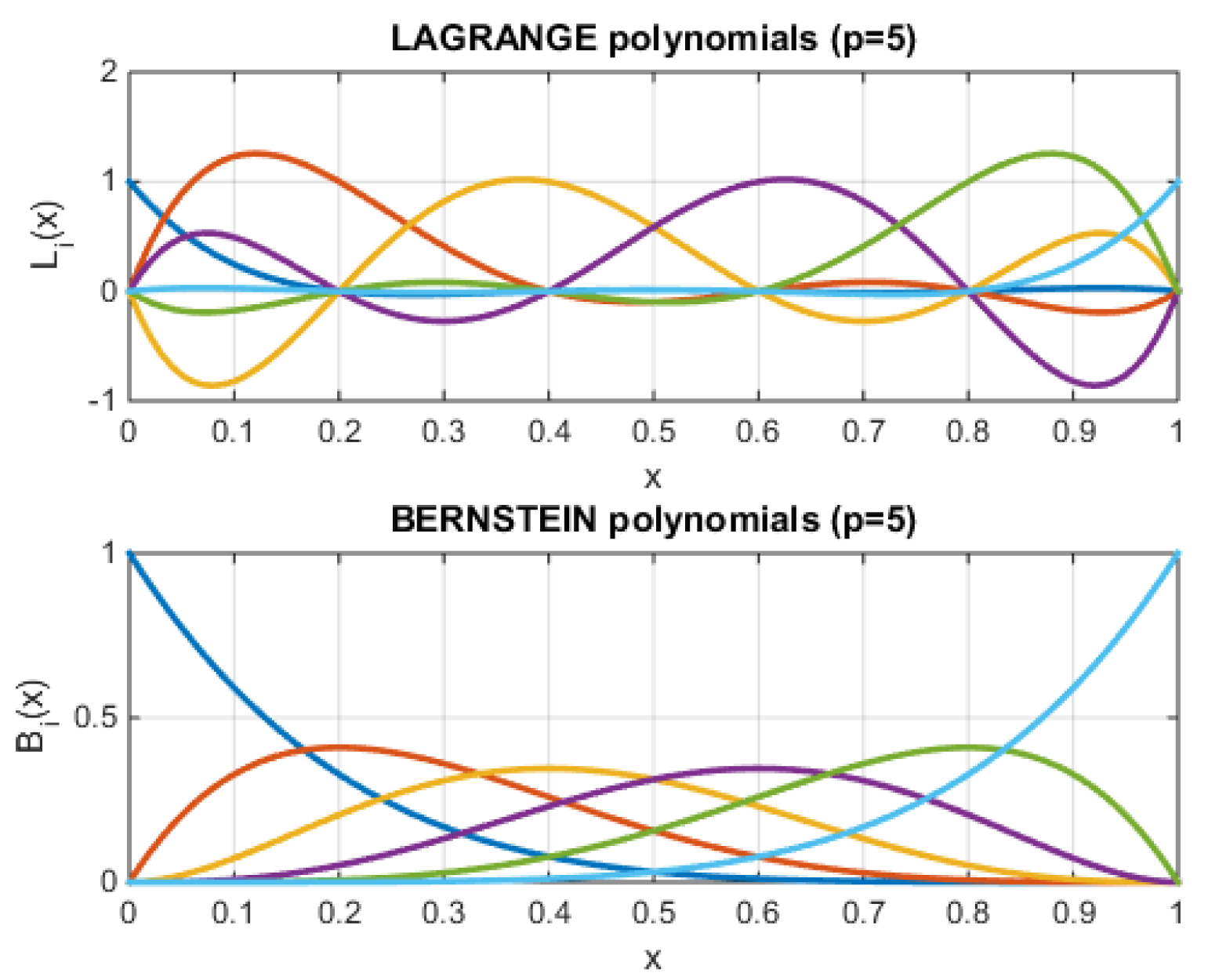
First, in Figure A1 we compare the polynomials of degree

p = 5

. One may observe that:

Lagrange polynomials $L_{i} (x)$ equal to the unity at the nodal points to which they are associated, and vanish at all the rest nodal points, i.e., they fulfil the condition $L_{i} (x_{j}) = δ_{i j}$ , where $δ_{i j}$ is Kronecker’s delta. They take positive and negative values and can be even larger than unity.
Bernstein polynomials $B_{i} (x)$ are non-negative functions, which are less or equal to the unity. The maxima of these functions appear subdivide the interval in $p$ equal spans.

Figure A1. Lagrange and Bernstein polynomials of degree

p = 5

Figure A1. Lagrange and Bernstein polynomials of degree

p = 5

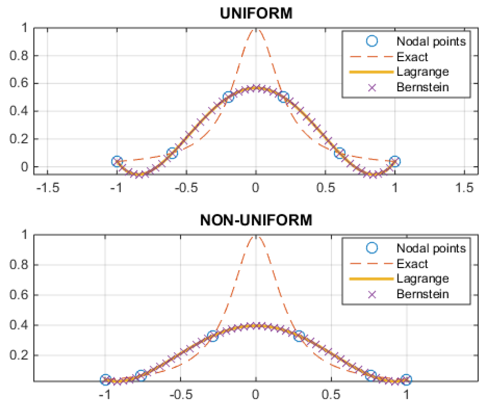
Second, let us use the above two functional sets to approximate the well-known Runge function

u (x) = 1 / (1 + 25 x^{2})

. In this context, using a uniform set of six (i.e.

p + 1

) nodal points: x(i): i = 0, 1/5, 2/5, 3/5, 4/5, 1, and then a non-uniform set, which are shown by blue-coloured circles, both functional sets are identical each other and fail, as clearly shown in Figure A2.

Figure A2. Approximation of Runge’s function using Lagrange and Bernstein polynomials of degree

p = 5

Figure A2. Approximation of Runge’s function using Lagrange and Bernstein polynomials of degree

p = 5

Appendix B: Global shape functions based on Lagrange polynomials

Figure B1. Quasi tensor-product element (25 nodes).

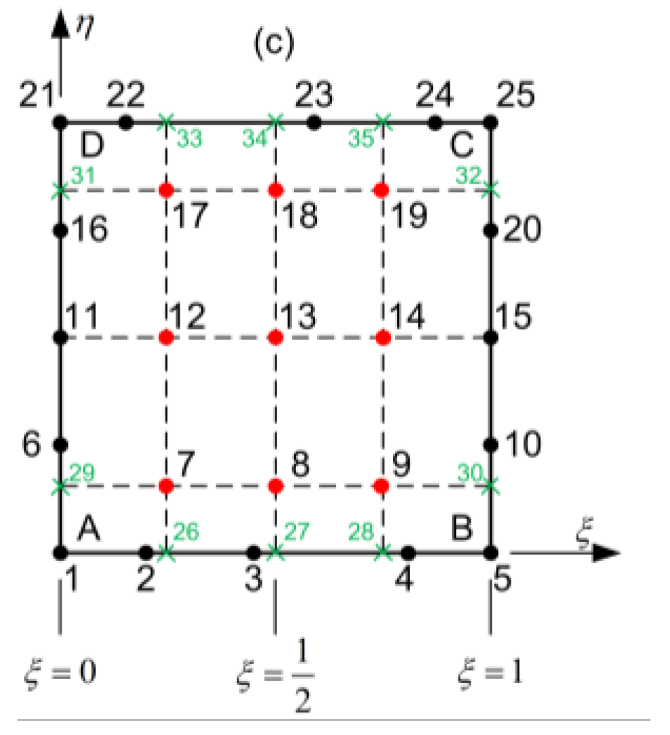
For the 25-node element shown in Figure B1, the global shape functions are produced by the implementation of the following Boolean sum:

u (ξ, η) = P_{ξ} + P_{η} - P_{ξ η}

(B.1)

where the three projectors are given as (see, Refs. [4-7]). In more detail, we have:

Toward the $ξ$ -axis:

$\begin{array}{l} P_{ξ} & = E_{0} (ξ) [L_{0}^{A D} (η) U_{1} + L_{1}^{A D} (η) U_{6} + L_{2}^{A D} (η) U_{11} + L_{3}^{A D} (η) U_{16} + L_{4}^{A D} (η) U_{21}] \\ + E_{1} (ξ) [L_{0}^{ξ = \frac{1}{4}} (η) U_{26} + L_{1}^{ξ = \frac{1}{4}} (η) U_{7} + L_{2}^{ξ = \frac{1}{4}} (η) U_{12} + L_{3}^{ξ = \frac{1}{4}} (η) U_{17} + L_{4}^{ξ = \frac{1}{4}} (η) U_{33}] \\ + E_{2} (ξ) [L_{0}^{ξ = \frac{2}{4}} (η) U_{27} + L_{1}^{ξ = \frac{2}{4}} (η) U_{8} + L_{2}^{ξ = \frac{2}{4}} (η) U_{13} + L_{3}^{ξ = \frac{2}{4}} (η) U_{18} + L_{4}^{ξ = \frac{2}{4}} (η) U_{34}] \\ + E_{3} (ξ) [L_{0}^{ξ = \frac{3}{4}} (η) U_{28} + L_{1}^{ξ = \frac{3}{4}} (η) U_{9} + L_{2}^{ξ = \frac{3}{4}} (η) U_{14} + L_{3}^{ξ = \frac{3}{4}} (η) U_{19} + L_{4}^{ξ = \frac{3}{4}} (η) U_{35}] \\ + E_{4} (ξ) [L_{0}^{B C} (η) U_{5} + L_{1}^{B C} (η) U_{10} + L_{2}^{B C} (η) U_{15} + L_{3}^{B C} (η) U_{20} + L_{4}^{B C} (η) U_{25}] \end{array}$

(B.2)
Toward the $η$ -axis:

$\begin{array}{l} P_{η} & = E_{0} (η) [L_{0}^{A B} (ξ) U_{1} + L_{1}^{A B} (η) U_{2} + L_{2}^{A B} (ξ) U_{3} + L_{3}^{A B} (ξ) U_{4} + L_{4}^{A B} (ξ) U_{5}] \\ + E_{1} (η) [L_{0}^{η = \frac{1}{4}} (ξ) U_{26} + L_{1}^{η = \frac{1}{4}} (ξ) U_{7} + L_{2}^{η = \frac{1}{4}} (ξ) U_{12} + L_{3}^{η = \frac{1}{4}} (ξ) U_{17} + L_{4}^{η = \frac{1}{4}} (ξ) U_{33}] \\ + E_{2} (η) [L_{0}^{η = \frac{2}{4}} (ξ) U_{27} + L_{1}^{η = \frac{2}{4}} (ξ) U_{8} + L_{2}^{η = \frac{2}{4}} (ξ) U_{13} + L_{3}^{η = \frac{2}{4}} (ξ) U_{18} + L_{4}^{η = \frac{2}{4}} (ξ) U_{34}] \\ + E_{3} (η) [L_{0}^{η = \frac{3}{4}} (ξ) U_{28} + L_{1}^{η = \frac{3}{4}} (ξ) U_{9} + L_{2}^{η = \frac{3}{4}} (ξ) U_{14} + L_{3}^{η = \frac{3}{4}} (ξ) U_{19} + L_{4}^{η = \frac{3}{4}} (ξ) U_{35}] \\ + E_{4} (η) [L_{0}^{D C} (ξ) U_{5} + L_{1}^{D C} (ξ) U_{10} + L_{2}^{D C} (ξ) U_{15} + L_{3}^{D C} (ξ) U_{20} + L_{4}^{D C} (ξ) U_{25}] \end{array}$

(B.3)
Tensor product:

$\begin{array}{l} P_{ξ η} & = E_{0} (ξ) E_{0} (η) U_{1} + E_{1} (ξ) E_{0} (η) U_{26} + E_{2} (ξ) E_{0} (η) U_{27} + E_{3} (ξ) E_{0} (η) U_{28} + E_{4} (ξ) E_{0} (η) U_{5} \\ + E_{0} (ξ) E_{1} (η) U_{29} + E_{1} (ξ) E_{1} (η) U_{7} + E_{2} (ξ) E_{1} (η) U_{8} + E_{3} (ξ) E_{1} (η) U_{9} + E_{4} (ξ) E_{1} (η) U_{30} \\ + E_{0} (ξ) E_{2} (η) U_{11} + E_{1} (ξ) E_{2} (η) U_{12} + E_{2} (ξ) E_{2} (η) U_{13} + E_{3} (ξ) E_{2} (η) U_{14} + E_{4} (ξ) E_{2} (η) U_{15} \\ + E_{0} (ξ) E_{3} (η) U_{31} + E_{1} (ξ) E_{3} (η) U_{17} + E_{2} (ξ) E_{3} (η) U_{18} + E_{3} (ξ) E_{3} (η) U_{19} + E_{4} (ξ) E_{3} (η) U_{32} \\ + E_{0} (ξ) E_{4} (η) U_{21} + E_{1} (ξ) E_{4} (η) U_{33} + E_{2} (ξ) E_{4} (η) U_{34} + E_{3} (ξ) E_{4} (η) U_{35} + E_{4} (ξ) E_{4} (η) U_{25} . \end{array}$

(B.4)

In the above three equations (B.2) to (B.4), the artificial nodes are denoted by green-coloured subscripts. After the substitution of these three equations into the Boolean sum given by Equation (B.1), the artificial terms are eventually cancelled. After factorization, the global shape functions are found as follows:

\begin{array}{l} N_{1} (ξ, η) = E_{0} (ξ) L_{0}^{A D} (η) + L_{0}^{A B} (ξ) E_{0} (η) - E_{0} (ξ) E_{0} (η), \\ N_{2} (ξ, η) = L_{1}^{A B} (ξ) E_{0} (η), \\ N_{3} (ξ, η) = L_{2}^{A B} (ξ) E_{0} (η), \\ N_{4} (ξ, η) = L_{3}^{A B} (ξ) E_{0} (η), \\ N_{5} (ξ, η) = E_{4} (ξ) L_{0}^{B C} (η) + L_{4}^{A B} (ξ) E_{0} (η) - E_{4} (ξ) E_{0} (η), \\ N_{6} (ξ, η) = E_{0} (ξ) L_{1}^{A D} (η), \\ N_{7} (ξ, η) = E_{1} (ξ) E_{1} (η), \\ N_{8} (ξ, η) = E_{2} (ξ) E_{1} (η), \\ N_{9} (ξ, η) = E_{3} (ξ) E_{1} (η), \\ N_{10} (ξ, η) = E_{4} (ξ) L_{1}^{B C} (η), \\ N_{11} (ξ, η) = E_{0} (ξ) L_{2}^{A D} (η), \\ N_{12} (ξ, η) = E_{1} (ξ) E_{2} (η), \\ N_{13} (ξ, η) = E_{2} (ξ) E_{2} (η), \\ N_{14} (ξ, η) = E_{3} (ξ) E_{2} (η), \\ N_{15} (ξ, η) = E_{4} (ξ) L_{2}^{B C} (η), \\ N_{16} (ξ, η) = E_{0} (ξ) L_{3}^{A D} (η), \\ N_{17} (ξ, η) = E_{1} (ξ) E_{3} (η), \\ N_{18} (ξ, η) = E_{2} (ξ) E_{3} (η), \\ N_{19} (ξ, η) = E_{3} (ξ) E_{3} (η), \\ N_{20} (ξ, η) = E_{4} (ξ) L_{3}^{B C} (η), \\ N_{21} (ξ, η) = E_{0} (ξ) L_{4}^{A D} (η) + L_{0}^{D C} (ξ) E_{4} (η) - E_{0} (ξ) E_{4} (η), \\ N_{22} (ξ, η) = L_{1}^{D C} (ξ) E_{4} (η), \\ N_{23} (ξ, η) = L_{2}^{D C} (ξ) E_{4} (η), \\ N_{24} (ξ, η) = L_{3}^{D C} (ξ) E_{4} (η), \\ N_{25} (ξ, η) = E_{4} (ξ) L_{4}^{B C} (η) + L_{4}^{D C} (ξ) E_{4} (η) - E_{4} (ξ) E_{4} (η) . \end{array}

(B.5)

Obviously, the global shape functions fulfil the series expansion:

u (ξ, η) = \sum_{j = 1}^{25} N_{j} (ξ, η) U_{j}

(B.6)

where

U_{j}, j = 1, \dots, 25

are the nodal values.

They also have the partition of unity property:

\sum_{j = 1}^{25} N_{j} (ξ, η) = 1, \forall ξ, η) \in [0, 1] \times [0, 1],

(B.7)

as well as the Kronecker delta property:

N_{i} (ξ_{j}, η_{j}) = δ_{i j} = \{\begin{cases} 1 if i = j \\ 0 if i \neq j \end{cases},

(B.8)

Appendix C: Derivation of formula for the Refinement

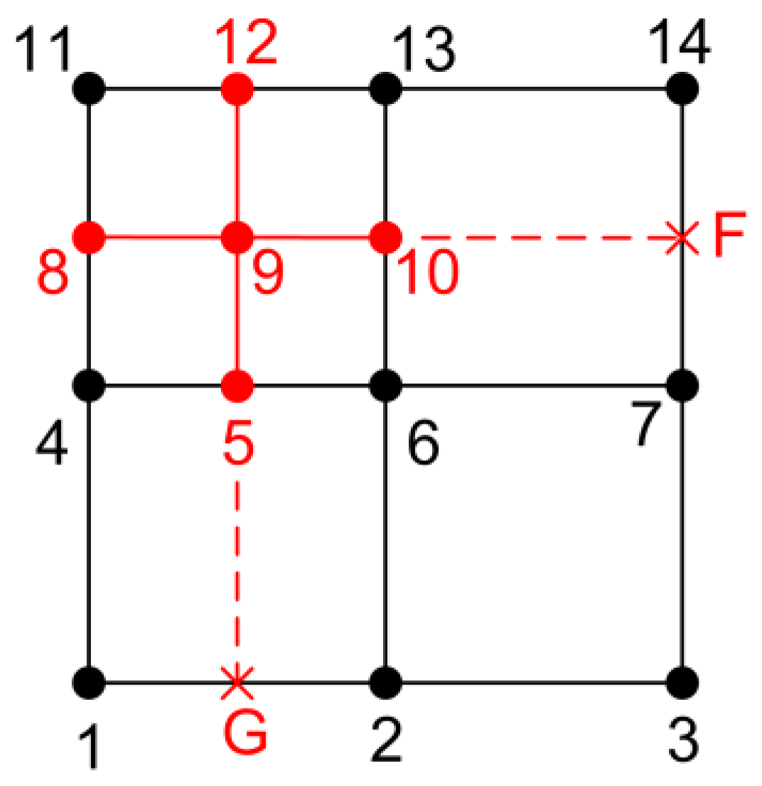
To derive the closed-form expression for the refinement, we extend the segments 12-9-5 and 8-9-10 until they intersect the boundary at the points G and F, respectively. Then we receive a full tensor product of 4 × 4 = 16 points, of which (G, F) are artificial (auxiliary) and will be eventually eliminated as follows:

Figure C1. Tensor-product configuration for performing the projectors.

The projector toward the ξ-axis is:

\begin{array}{l} P_{ξ} & = E_{0} (ξ) [L_{0}^{(3)} (η) U_{1} + L_{\frac{2}{4}}^{(3)} (η) U_{4} + L_{\frac{3}{4}}^{(3)} (η) U_{8} + L_{1}^{(3)} (η) U_{11}] \\ + E_{\frac{1}{4}} (ξ) [L_{0}^{(3)} (η) U_{G} + L_{\frac{2}{4}}^{(3)} (η) U_{5} + L_{\frac{3}{4}}^{(3)} (η) U_{9} + L_{1}^{(3)} (η) U_{12}] \\ + E_{\frac{2}{4}} (ξ) [L_{0}^{(3)} (η) U_{2} + L_{\frac{2}{4}}^{(3)} (η) U_{6} + L_{\frac{3}{4}}^{(3)} (η) U_{10} + L_{1}^{(3)} (η) U_{13}] \\ + E_{1} (ξ) [L_{0}^{(2)} (η) U_{3} + L_{\frac{1}{2}}^{(2)} (η) U_{7} + L_{1}^{(2)} (η) U_{14}] \end{array}

(C.1)

Note that the interpolation along the right vertical edge BC is based on the actual nodes (3, 7, and 14) along it, and not on the auxiliary node F.

The projector toward the η-axis is:

\begin{array}{l} P_{η} & = E_{0} (η) [L_{0}^{(2)} (ξ) U_{1} + L_{\frac{1}{2}}^{(2)} (ξ) U_{2} + L_{1}^{(2)} (ξ) U_{3}] \\ + E_{\frac{1}{2}} (η) [L_{0}^{(3)} (ξ) U_{4} + L_{\frac{1}{4}}^{(3)} (ξ) U_{5} + L_{\frac{2}{4}}^{(3)} (ξ) U_{6} + L_{1}^{(3)} (ξ) U_{7}] \\ + E_{\frac{3}{4}} (η) [L_{0}^{(3)} (ξ) U_{8} + L_{\frac{1}{4}}^{(3)} (ξ) U_{9} + L_{\frac{2}{4}}^{(3)} (ξ) U_{10} + L_{1}^{(3)} (ξ) U_{F}] \\ + E_{1} (η) [L_{0}^{(3)} (ξ) U_{11} + L_{\frac{1}{4}}^{(3)} (ξ) U_{12} + L_{\frac{2}{4}}^{(3)} (ξ) U_{13} + L_{1}^{(3)} (ξ) U_{14}] \end{array}

(C.2)

Note that the interpolation along the bottom edge AB is based on the actual nodes (1, 2 and 3) along it, and not on the auxiliary node G.

The tensor-product projector is:

\begin{array}{l} P_{ξ η} & = E_{0} (ξ) E_{0} (η) U_{1} + E_{\frac{1}{4}} (ξ) E_{0} (η) U_{G} + E_{\frac{2}{4}} (ξ) E_{0} (η) U_{2} + E_{1} (ξ) E_{0} (η) U_{3} \\ + E_{0} (ξ) E_{\frac{1}{2}} (η) U_{4} + E_{\frac{1}{4}} (ξ) E_{\frac{1}{2}} (η) U_{5} + E_{\frac{2}{4}} (ξ) E_{\frac{1}{2}} (η) U_{6} + E_{1} (ξ) E_{\frac{1}{2}} (η) U_{7} \\ + E_{0} (ξ) E_{\frac{3}{4}} (η) U_{8} + E_{\frac{1}{4}} (ξ) E_{\frac{3}{4}} (η) U_{9} + E_{\frac{2}{4}} (ξ) E_{\frac{3}{4}} (η) U_{10} + E_{1} (ξ) E_{\frac{3}{4}} (η) U_{F} \\ + E_{0} (ξ) E_{1} (η) U_{11} + E_{\frac{1}{4}} (ξ) E_{1} (η) U_{12} + E_{\frac{2}{4}} (ξ) E_{1} (η) U_{13} + E_{1} (ξ) E_{1} (η) U_{14} \end{array}

(C.3)

One may observe that the auxiliary values (

U_{G}

, and

U_{F}

) appear in Equations (C.1) and (C.2), respectively, whereas both of them appear once in Equation (C.3). Therefore, when performing the Boolean sum

P_{ξ} + P_{η} - P_{ξ η}

, all the terms including the auxiliary values (

U_{G}

, and

U_{F}

) are cancelled, and thus the final expression (see, Equation (48)) includes only the 14 nodal values,

U_{1}

U_{14}

References

Farin, G.; Hoschek, J.; Kim, M.S. Handbook of computer aided geometric design; Elsevier: North-Holland, 2002. [Google Scholar]
Piegl, L.; Tiller, W. The NURBS Book. Springer, Berlin, Germany, 1997. Springer: Berlin, Germany, 1997. [Google Scholar]
Coons, S.A. Surfaces for computer aided design of space form, Project MAC, MIT(1964), revised for MAC-TR-41 (1967). Springfield: USA. Available online: http://publications.csail.mit.edu/lcs/pubs/pdf/MIT-LCS-TR-041.pdf.
Gordon, W.J. Spline-blended surface interpolation through curve networks. Indiana Univ. Math J 1969, 18, 931–952. Available online: http://www.iumj.indiana.edu//IUMJ/FULLTEXT/1969/18/18068. [CrossRef]
Gordon, W.J. Blending functions methods of bivariate and multivariate interpolation and approximation. SIAM J Numer Anal 1971, 8, 158–177. [Google Scholar] [CrossRef]
Gordon, W.J.; Hall, C.A. Construction of curvilinear co-ordinate systems and application to mesh generation. Int J Numer Meth Eng 1973, 7, 461–477. [Google Scholar] [CrossRef]
Gordon, W.J.; Hall, C.A. Transfinite element methods: Blending-function interpolation over arbitrary curved element domains. Numerische Mathematik 1973, 21, 109–129. [Google Scholar] [CrossRef]
Cavendish, J.C.; Gordon, W.J.; Hall, C.A. Ritz-Galerkin approximations in blending function spaces. Numerische Mathematik 1976, 25, 155–178. [Google Scholar] [CrossRef]
Cavendish, J.C.; Gordon, W.J.; Hall, C.A. Substructured macro elements based on locally blending interpolation. Int J Numer Meth Eng 1977, 11, 1405–1421. [Google Scholar] [CrossRef]
Cavendish, W.J.; Hall, C.A. A new class of transitional blended finite elements for the analysis of solid structures. Int J Numer Meth Eng 1984, 28, 241–253. [Google Scholar] [CrossRef]
Zhaobei, Z.; Zhiqiang, X. Coons’ surface method for formulation of finite element of plates and shells. Comput Struct 1987, 27, 79–88. [Google Scholar] [CrossRef]
Kanarachos, A.; Deriziotis, D. On the solution of Laplace and and wave propagation problems using ‘C-elements’. Finite Elem Anal Des 1989, 5, 97–109. [Google Scholar] [CrossRef]
Provatidis, C.; Kanarachos, A. Performance of a macro-FEM approach using global interpolation (Coons’) functions in axisymmetric potential problems. Comput Struct 2001, 79, 1769–1779. [Google Scholar] [CrossRef]
Hughes, T.J.R.; Cottrell, J.A.; Bazilevs, Y. Isogeometric analysis: CAD, finite elements, NURBS, exact geometry and mesh refinement. Comput. Methods Appl. Mech. Eng. 2005, 194, 4135–4195. [Google Scholar] [CrossRef]
Cottrell, J.A.; Hughes, T.J.R.; Bazilevs, Y. Isogeometric analysis: towards integration of CAD and FEA; Wiley: Chichester, 2009. [Google Scholar]
Provatidis, C.G. Precursors of isogeometric analysis: Finite elements, Boundary elements, and Collocation methods; Springer: Cham, 2019. [Google Scholar]
Provatidis, C.G. Non-rational and rational transfinite interpolation using Bernstein polynomials. International Journal of Computational Geometry and Applications 2022, 32, 55–89. [Google Scholar] [CrossRef]
Lagrange J., L. Théorie des fonctions analytiques (in French); Courcier: Paris, 1813. [Google Scholar]
Schoenberg, I.J. Contributions to the problem of approximation of equidistant data by analytic functions, Part A.—On the problem of smoothing or graduation. A first class of analytic approximation formulae. Quarterly of Applied Mathematics 1946, 4, 45–99. [Google Scholar] [CrossRef]
Gasca, M.; Sauer, T. On the history of multivariate polynomial interpolation. Journal of Computational and Applied Mathematics 2000, 122, 23–35. [Google Scholar] [CrossRef]
Davis, P. J. Interpolation and Approximation; Dover: New York, 1975. [Google Scholar]
Ralston, A.; Rabinowitz, P. A First Course in Numerical Analysis, 2nd edn.; Dover Publications: New York, 1978. [Google Scholar]
Bernstein, S.N. Demonstration du théorème de Weierstrass fondée sur le calcul des probabilités. Proc. Kharkow Math. Soc. 1912, 13, 1–2. [Google Scholar]
Lanczos, C. Trigonometric interpolation of empirical and analytical functions. J. Math. Phys. 1938, 17, 123–199. [Google Scholar] [CrossRef]
Bézier, P. Mathematical and practical possibilities of UNISURF. In Computer Aided Geometric Design; Barnhill, R.E., Riesenfel, R.F., Eds.; Academic Press, 1974; pp. 127–152. ISBN 9780120790500. [Google Scholar]
Provatidis, C.G. Two-dimensional elastostatic analysis using Coons-Gordon interpolation. Meccanica 2012, 47, 951–967. [Google Scholar] [CrossRef]
Micchelli, C.A. Interpolation of scattered data: Distance matrices and conditionally positive definite functions. Constr. Approx. 1986, 2, 11–22. [Google Scholar] [CrossRef]
Franke, R. Scattered data interpolation: tests of some methods. Math. Comp. 1982, 38, 381–200. [Google Scholar]
Kansa, E.J. Multiquadrics—A scattered data approximation scheme with applications to computational fluid-dynamics—I surface approximations and partial derivative estimates. Computers & Mathematics with Applications 1990, 19, 127–145. [Google Scholar]
Liu, Y.; Li, H. B-spline patches and transfinite interpolation method for PDE controlled simulation. J Syst Sci Complex 2012, 25, 348–361. [Google Scholar] [CrossRef]

Figure 2. Several types of structured transfinite elements. The black circles represent nodes (nodal points).

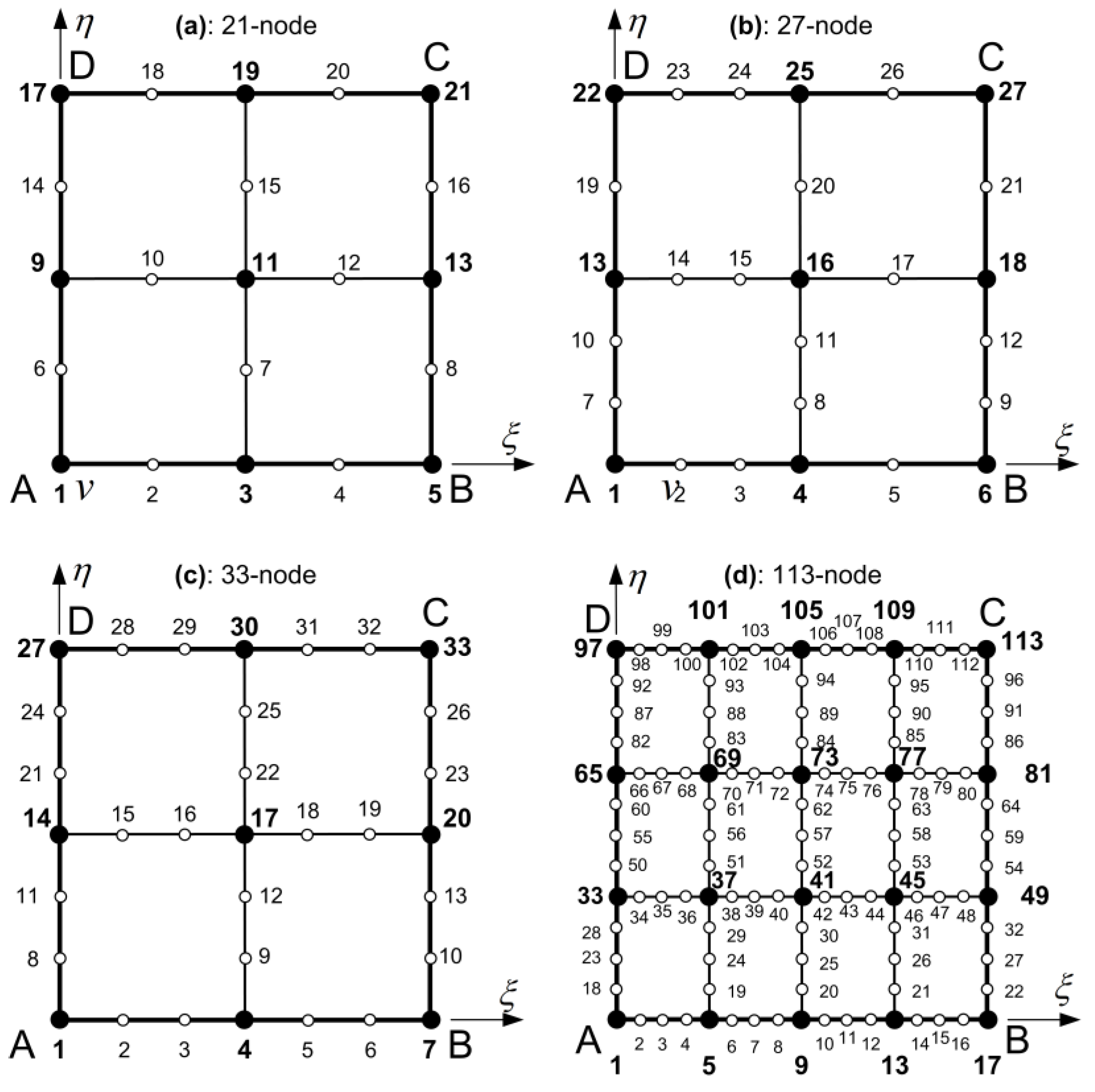
Figure 3. (a) Tensor-product and (b) distorted tensor-product transfinite elements (Si: vertical stations, Ti: horizontal stations).

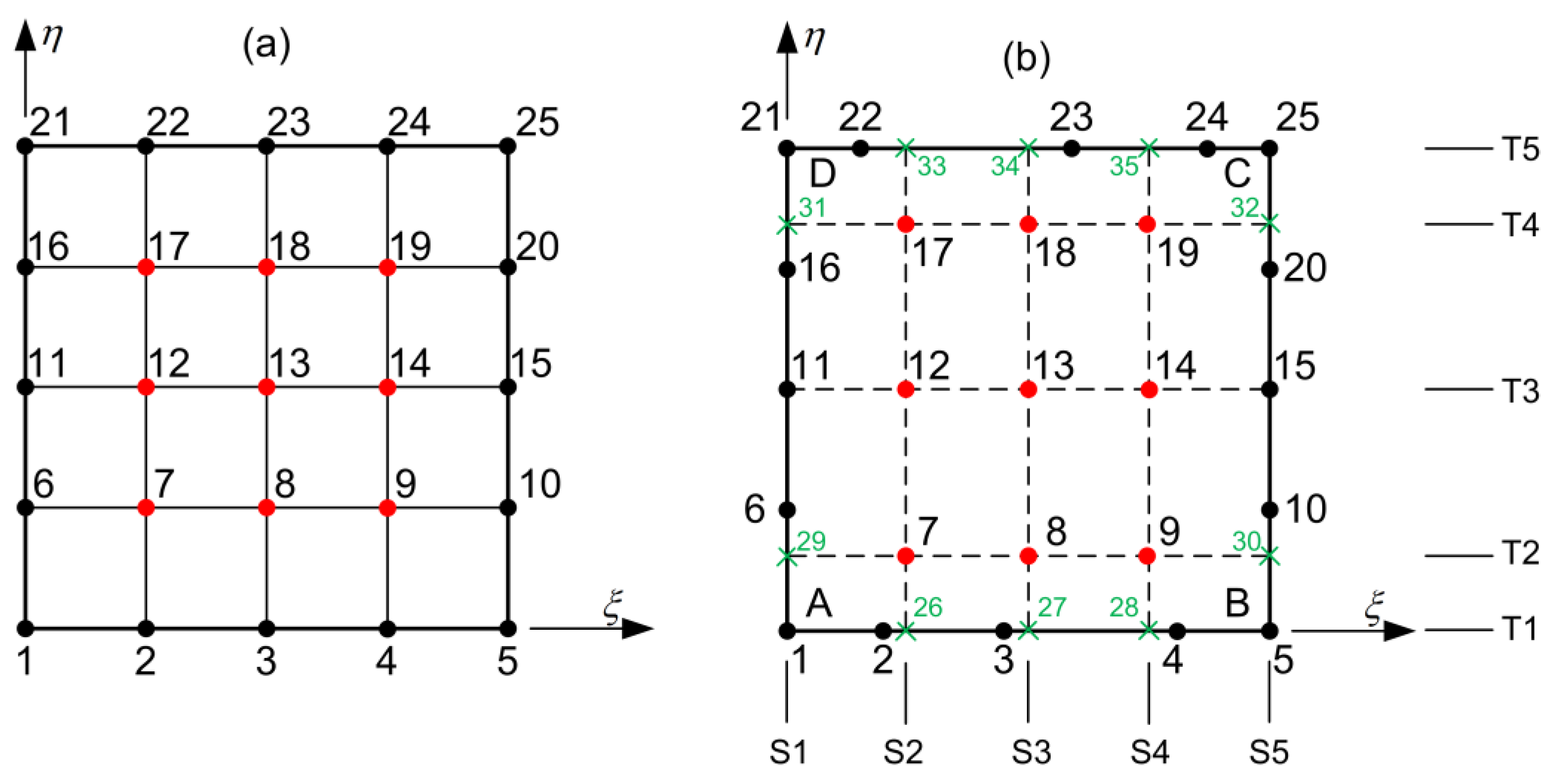
Figure 5. Global shape functions for the transfinite element of 21 DOFs. (a) Lagrange only, (b) Bernstein only, (c) B-spline of degree 3, (d) B-spline of degree 2.

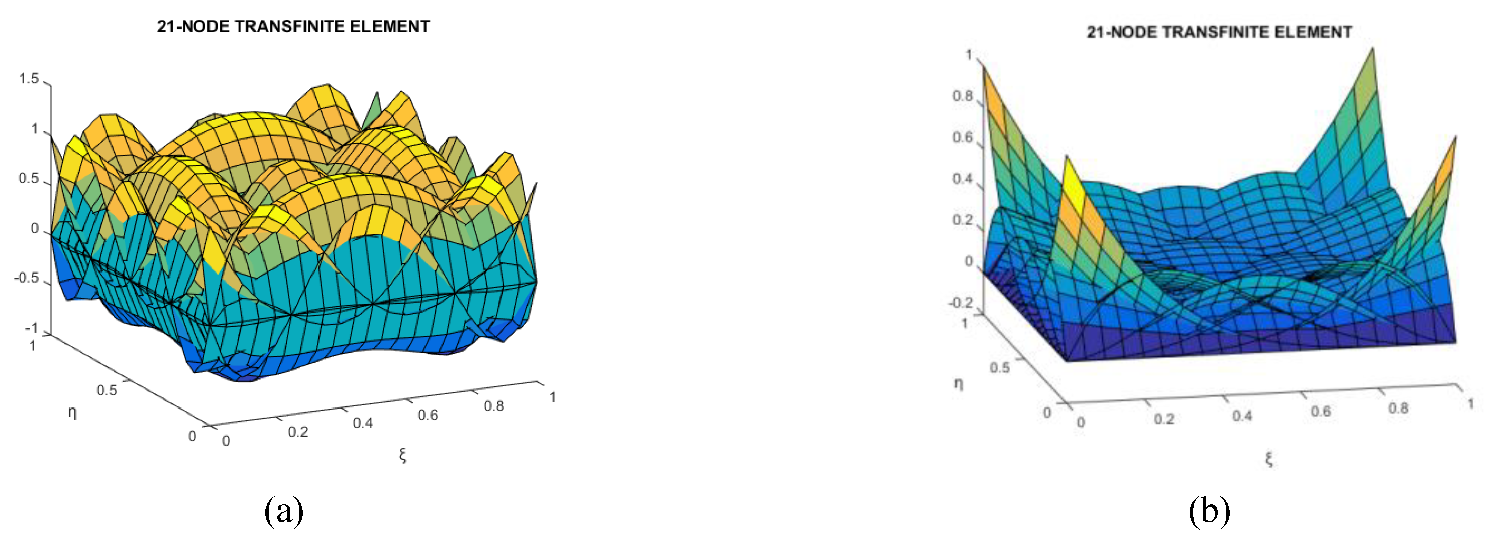
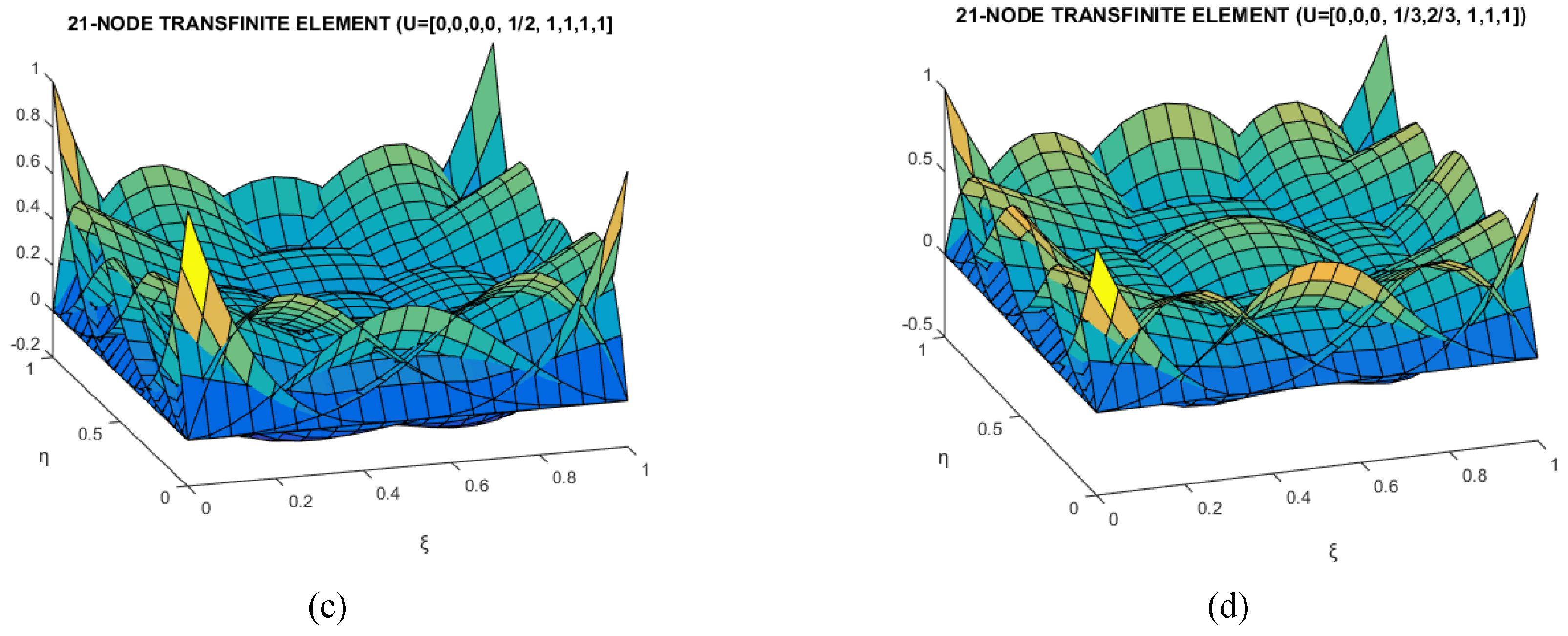
Figure 6. Global shape functions using (a) all-Lagrange polynomials, (b) all-Bernstein polynomials, and (c) mixed Bernstein polynomials-cubic B-splines for blending and trial functions, respectively.

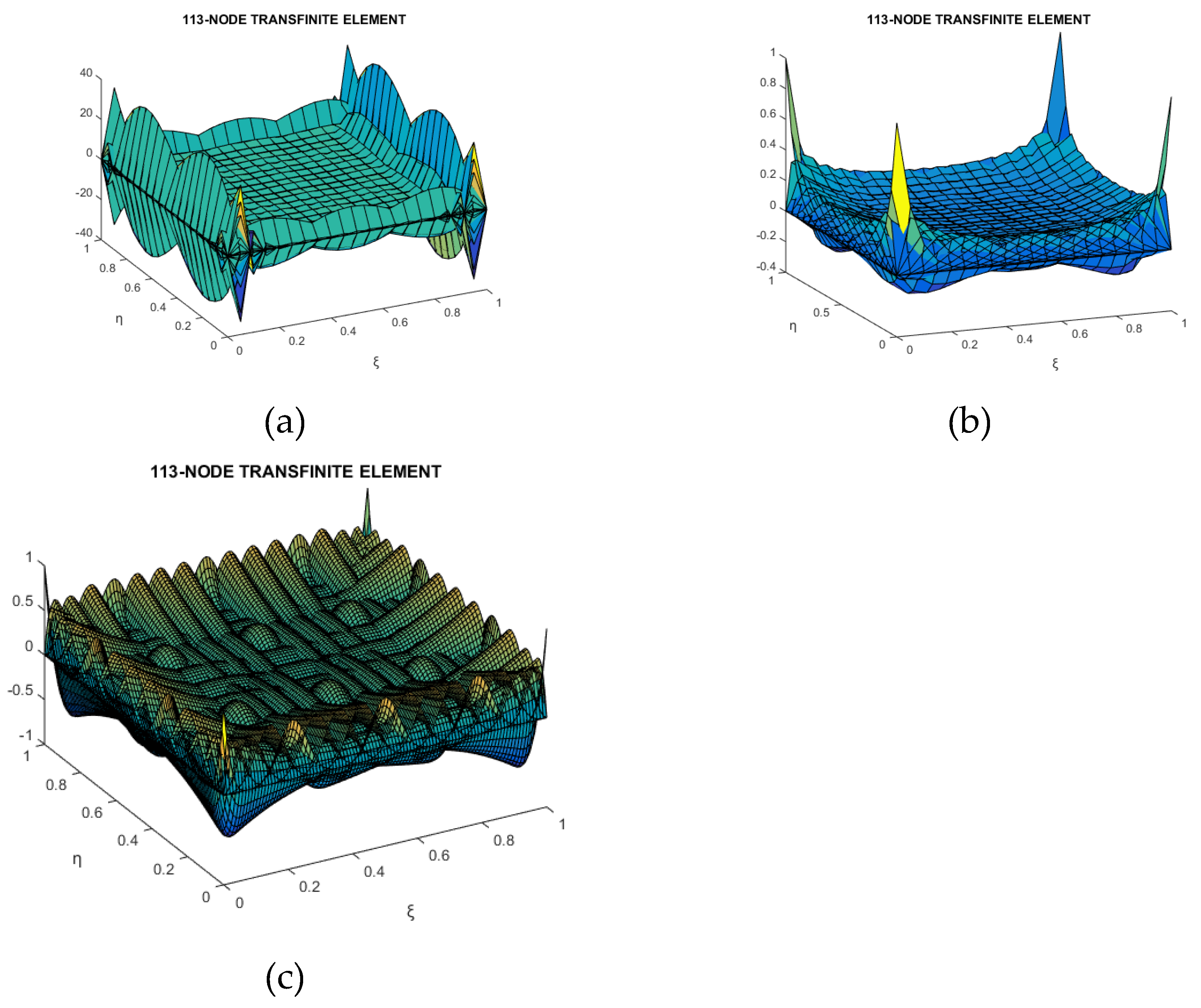
Figure 7. Shape functions of a 25-node distorted transfinite element using (a) Lagrange polynomials (b) Bernstein polynomials.

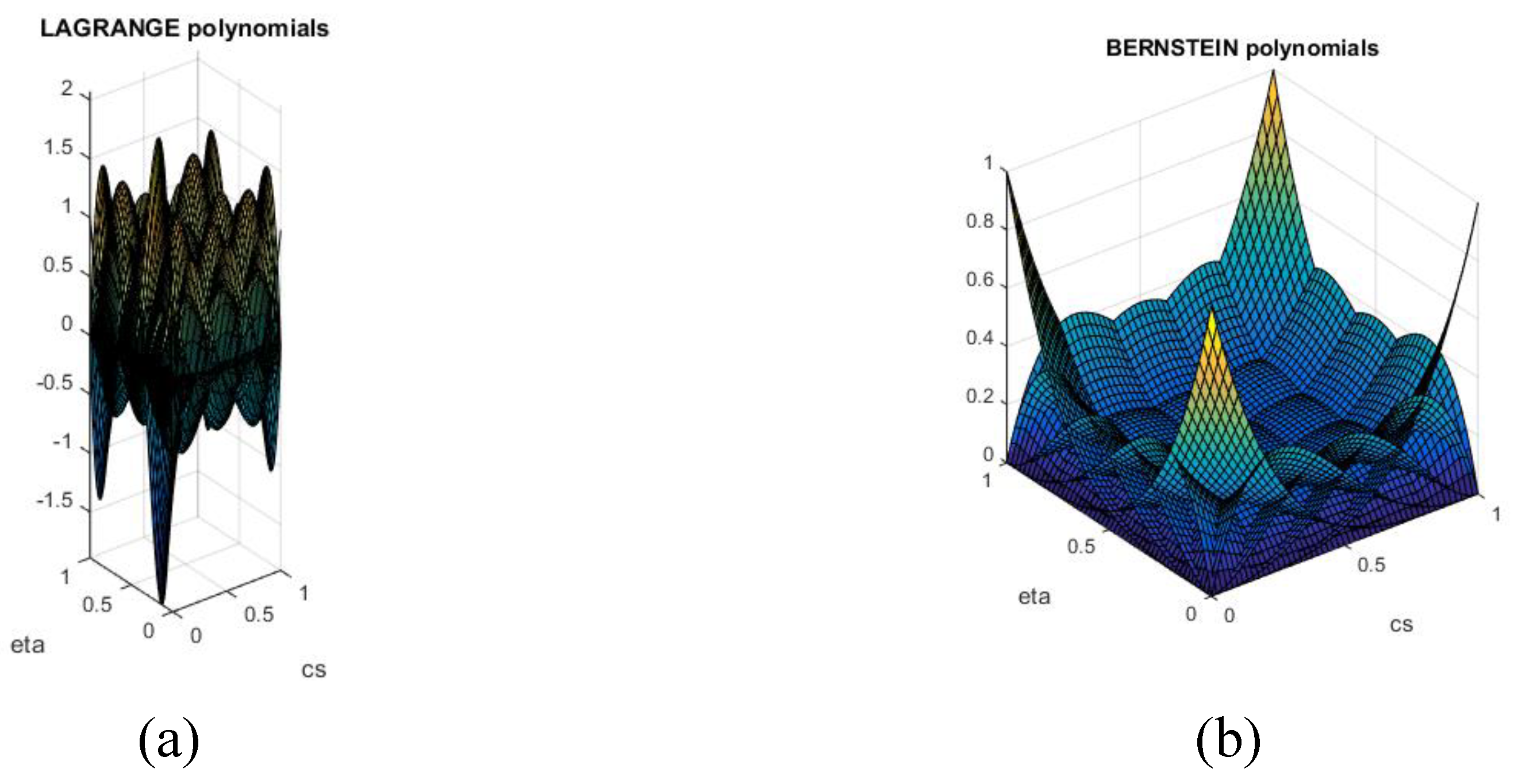
Figure 9. Refinement of patch ABCD.

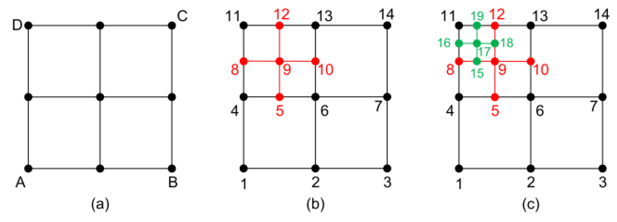
Figure 10. (a) Lagrange-based and (b) Bernstein-based transfinite elements, after the first refinement.

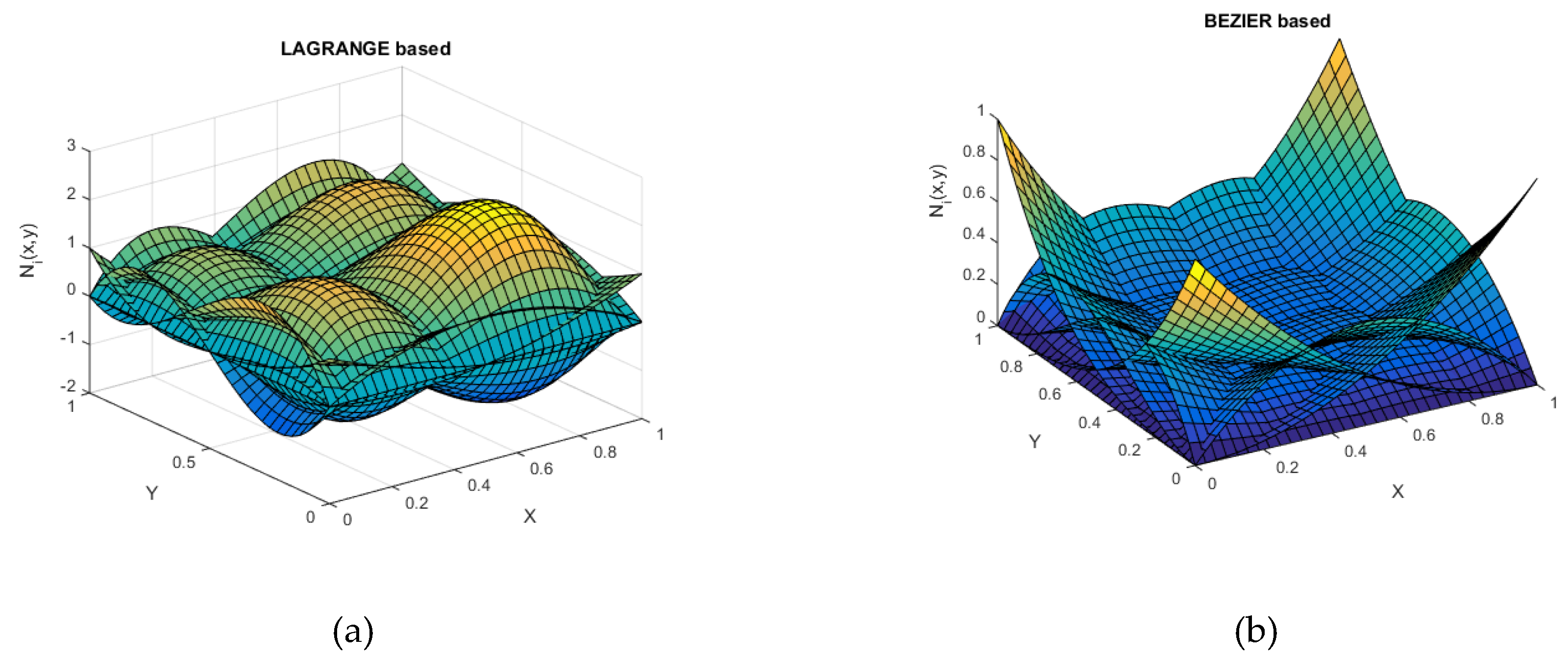
Figure 11. A non-tensor-product mesh with gaps.

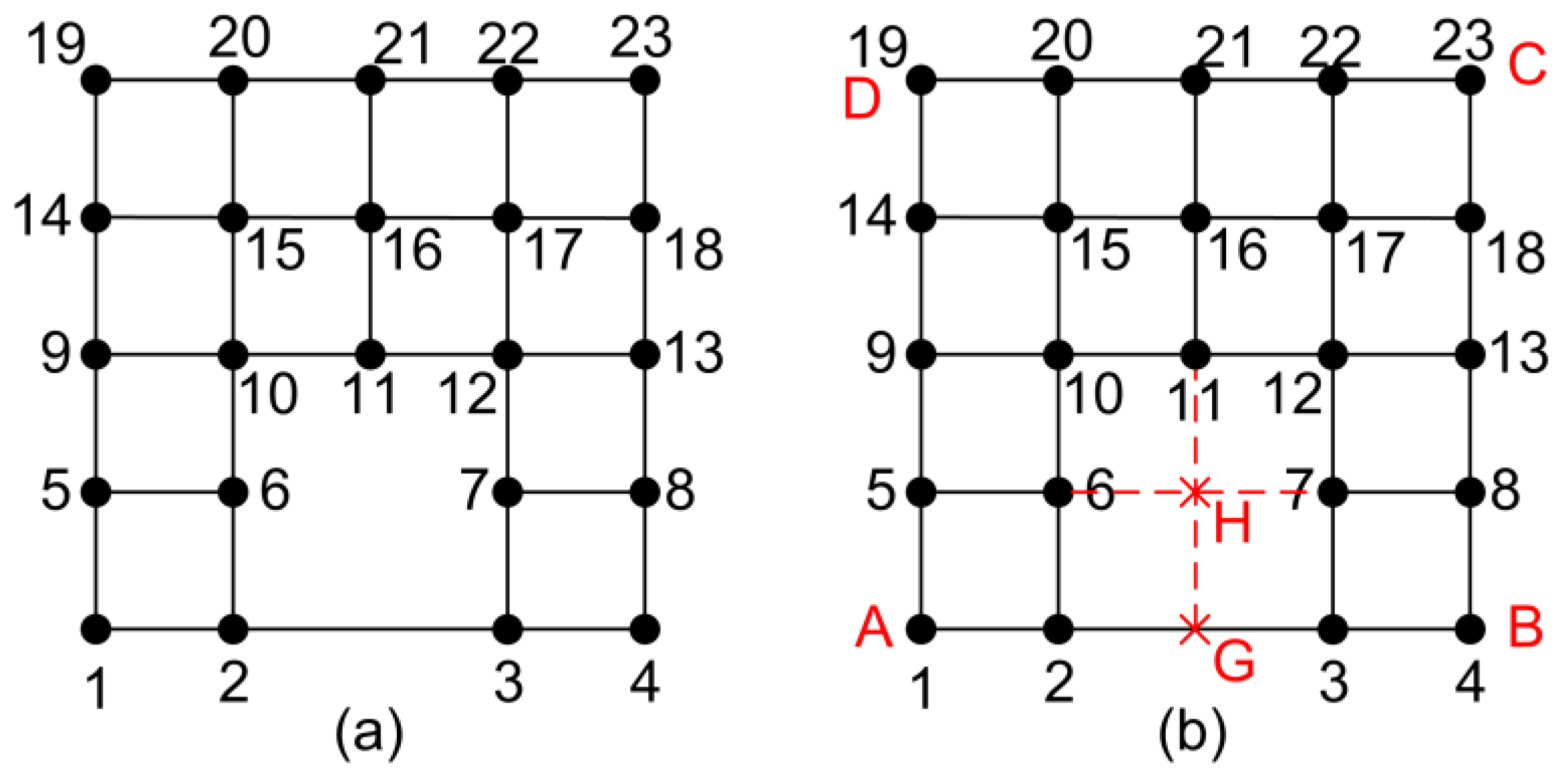
Figure 12. Global shape functions using (a) Lagrange polynomials and (b) Bernstein polynomials.

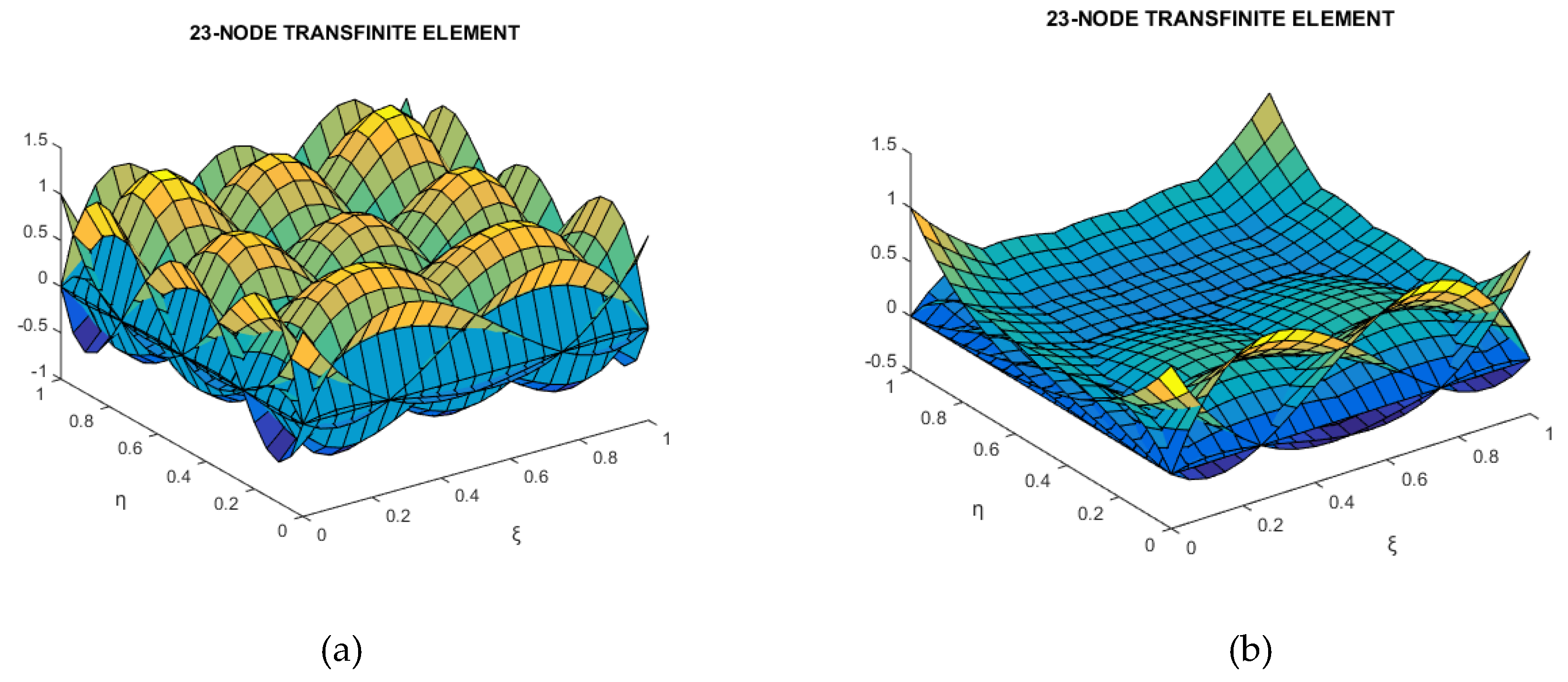
Figure 13. The analogue T-mesh.

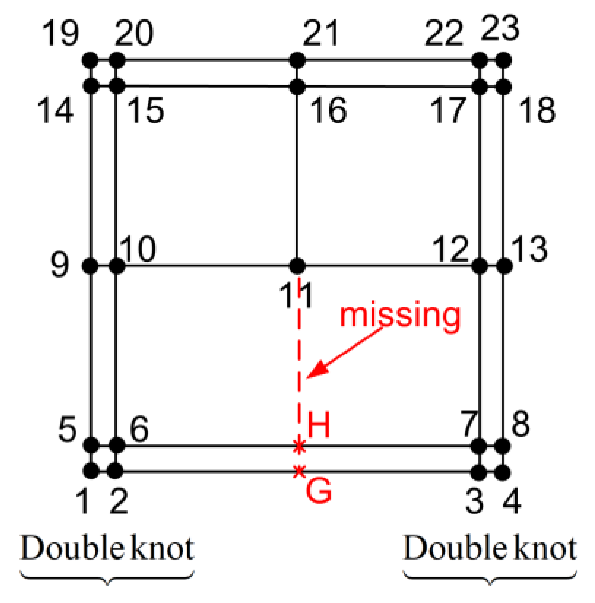
Figure 14. Global shape functions using (a) B-spline transfinite interpolation and (b) T-splines formulation.

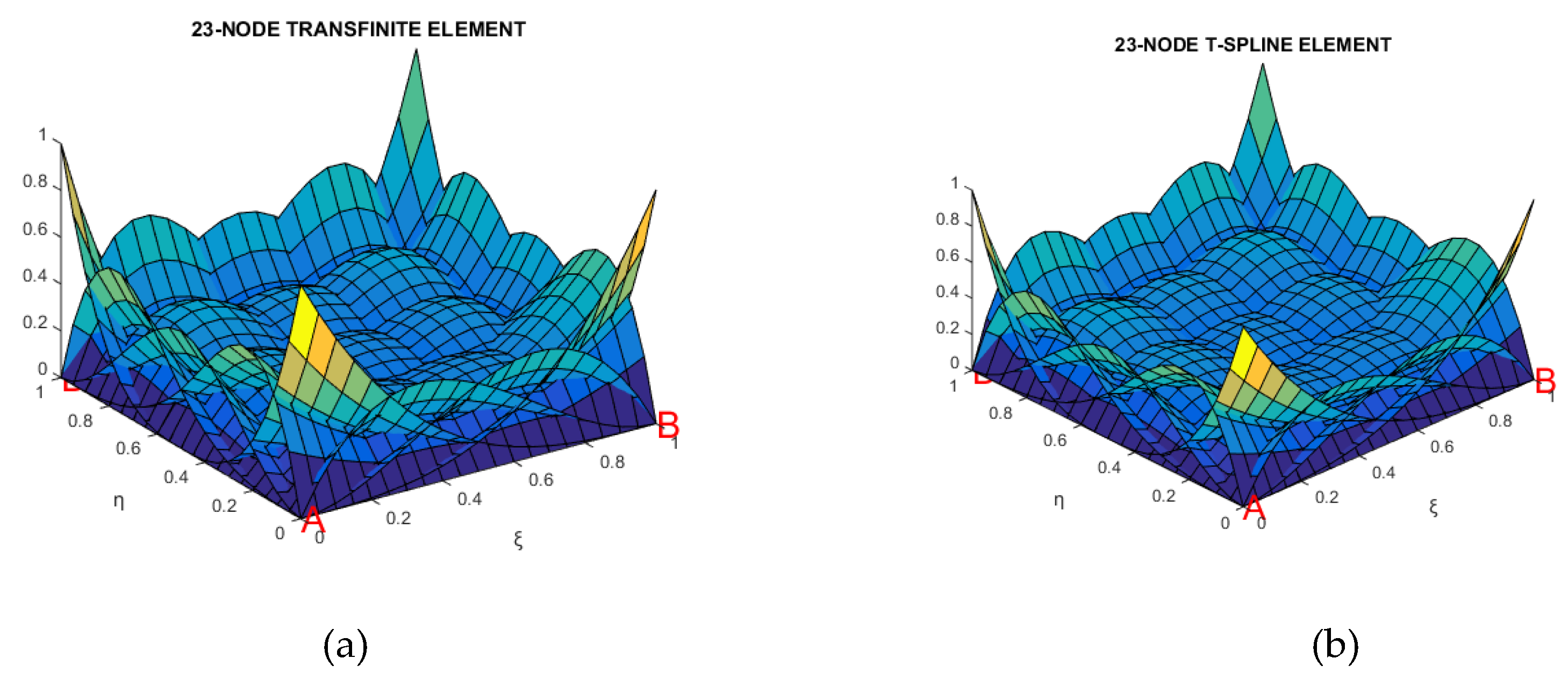
Figure 15. T-mesh of 14 nodes for (a) Lagrange polynomials, (b) after extension, (c) index space.

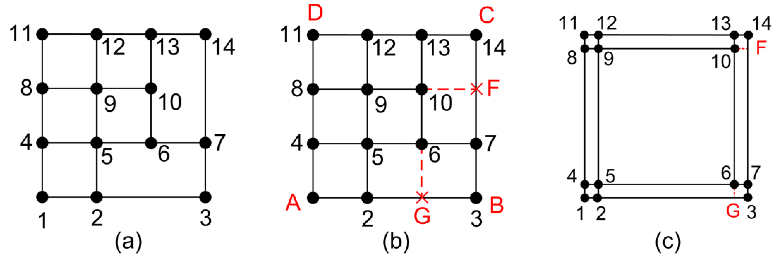
Figure 16. Shape functions using (a) Lagrange polynomials and (b) Bernstein polynomials.

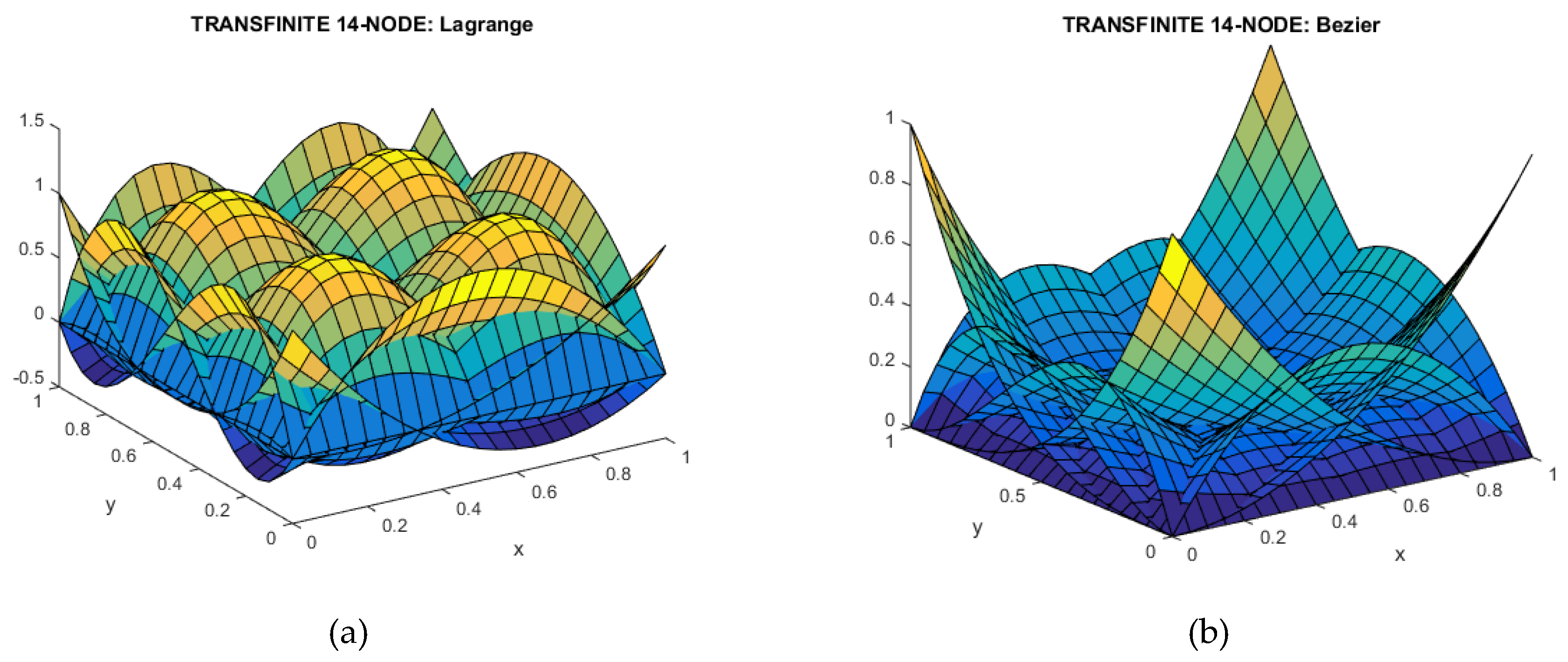
Table 1. L2 error-norm (in percent %) for the 21-node element.

	Functions		L2-norm (in %)
	BLENDING	TRIAL	L2-norm (in %)
1	Lagrange (p = 2)	Lagrange (p = 4)	0.5202
2	Bernstein (p = 2)	Bernstein (p = 4)	0.5202
3	Lagrange (p = 2)	B-splines (p = 3)	0.5223
4	Bernstein (p = 2)	B-splines (p = 3)	0.5223
5	Lagrange (p = 2)	B-splines (p = 2)	0.8690
6	Bernstein (p = 2)	B-splines (p = 2)	0.8690

Table 2. L2 error-norm (in percent %) for the 113-node element.

	Functions		L2-norm (in %)
	BLENDING	TRIAL	L2-norm (in %)
1	Lagrange (p_x = 4, p_y = 3)	Lagrange (p_x = 16, p_y = 12)	1.2326 × 10^-5
2	Bernstein (p_x = 4, p_y = 3)	Bernstein (p_x = 16, p_y = 12)	1.2326 × 10^-5
3	Lagrange (p_x = 4, p_y = 3)	B-splines (p = 3)	0.0013
4	Bernstein (p_x = 4, p_y = 3)	B-splines (p = 3)	0.0013

Table 3. L2-norm (in percent %).

CASE	Functions		L2-norm (in %)
CASE	BLENDING	TRIAL	L2-norm (in %)
1	Lagrange (p = 4)	Lagrange (p = 4)	0.4968
2	Bernstein (p = 4)	Bernstein (p = 4)	0.4968
3	Lagrange (p = 4)	B-splines (p = 3)	0.4840
4	Bernstein (p = 4)	B-splines (p = 3)	0.4841
5	Lagrange (p = 4)	B-splines (p = 2)	0.5003
6	Bernstein (p = 4)	B-splines (p = 2)	0.5006
7	B-splines (p = 2)	B-splines (p = 2)	0.8816
8	B-splines (p = 3)	B-splines (p = 3)	0.4848

Disclaimer/Publisher’s Note: The statements, opinions and data contained in all publications are solely those of the individual author(s) and contributor(s) and not of MDPI and/or the editor(s). MDPI and/or the editor(s) disclaim responsibility for any injury to people or property resulting from any ideas, methods, instructions or products referred to in the content.

© 2024 by the authors. Licensee MDPI, Basel, Switzerland. This article is an open access article distributed under the terms and conditions of the Creative Commons Attribution (CC BY) license (http://creativecommons.org/licenses/by/4.0/).

Copyright: This open access article is published under a Creative Commons CC BY 4.0 license, which permit the free download, distribution, and reuse, provided that the author and preprint are cited in any reuse.

Downloads

Views

Comments

Subscription

Notify me about updates to this article or when a peer-reviewed version is published.

MDPI Initiatives

Important Links

Choose an area of interest and we will send you notifications of new preprints at your preferred frequency.

Disclaimer

Transfinite Patches for Isogeometric Analysis

Abstract

Keywords:

Subject:

1. Introduction

2. Linear Blending Functions in Coons’ interpolation

2.1 Linear interpolation in the physical space

2.2. Linear interpolation in the parametric space

2.3. Projectors within a quadrilateral

2.4. Interpolation by a Boolean sum

3. Higher-order Blending Functions in Gordon’s (transfinite) interpolation

3.1. From Coons’ patch to Gordon’s patch theory

3.2. Transfinite interpolation

3.3. Tensor-product under the umbrella of transfinite interpolation

3.3.1. Historical note on univariate interpolation

3.3.2. Tensor product using Lagrange polynomials

3.3.3. Generalization of tensor product

4. Trial functions

4.1. Lagrange polynomials

4.2. Bernstein polynomials

4.3. Relationship between Lagrange and Bernstein polynomials

4.3.1. Uniform distribution of nodal points

4.3.2 Non-uniform distribution of nodal points

4.4 B-splines

4.5. Non-uniform Rational B-splines (NURBS)

5. Tensor-products of trial functions

5.1. Lagrange polynomials

5.2 Bernstein polynomials

5.3 . B-splines

5.4. NURBS approximation

6. The proposed Conjecture

6.1. Bernstein tensor-product elements

6.2. B-spline tensor-product elements

6.3. NURBS tensor-product elements

6.4. Overall evidence for tensor-product elements

6.5. Applications

6.5.1. The 21-node transfinite element

6.5.2. The 113-node transfinite element

7. Unstructured transfinite elements

7.1. Tensor-product-like 25-node element

7.1.1. Lagrange-polynomial based elements

7.1.2. Bernstein-polynomial based elements

7.2. Tensor-product-like 27-node element

8. Mesh Refinement

9. T-mesh like transfinite elements

9.1. Lagrange and Bernstein polynomials

9.2. B-spline blending and trial functions

10. Discussion

11. Conclusions

Author Contributions

Funding

Conflicts of Interest

Appendix A: Lagrange versus Bernstein polynomials

Appendix B: Global shape functions based on Lagrange polynomials

Appendix C: Derivation of formula for the Refinement

References

MDPI Initiatives

Important Links

Subscribe