Submitted:
18 December 2024
Posted:
19 December 2024
You are already at the latest version
Abstract
The research activity carried out has demonstrated how simulation tools developed through WebGIS3d digital platforms are capable of producing approximate forecasts on the effects of potentially catastrophic meteorological phenomena that may affect riverbeds in the territories observed. This work presents an analysis and simulation platform with graphic representation of the results in the form of three-dimensional animation. This methodology may represent a useful tool for all those bodies and organizations that need to create hypothetical scenarios for the management of emergencies related to flooding events of watercourses, especially in the areas of maximum hydrogeological vulnerability in the Italian territory. These scenarios are particularly useful in cases where watercourses are located near inhabited centers, industrial areas or strategic infrastructures, where the risk of material damage and danger to the population is greater. The simulation is based on the morphology of the land adjacent to the bed of the affected watercourse, taking elevation into account to determine the direction of expansion of the water mass.
Such scenarios are particularly useful in cases where watercourses are located near built-up areas, industrial areas or strategic infrastructures, where the risk of material damage and danger to the population is greater. The simulation is based on the morphology of the terrain adjacent to the affected watercourse bed, taking elevation into consideration to determine the direction of ex-pansion of the water mass.
A distinctive aspect of the platform is its extreme speed in the resolution of simulations, which also allows the tool to be used in real time. This means that during the occurrence of a meteoro-logical event, the platform can be used to monitor the evolution of the situation and predict the effects of any persistence of the phenomenon over time. This real-time forecasting capability is crucial for making quick and informed decisions, thus reducing reaction times and improving emergency management on the ground, with a potential positive impact on the safety of the population and the protection of infrastructure.
Keywords:
web-GIS 3d
; Hydraulic Analysis and simulation
; Hydrogeological Analysis and Simulation
1. Introduction
The Italian territory has more than 1,200 watercourses, which represent a fundamental element of the country’s natural landscape and hydrographic heritage. This extensive river network not only models the territory, but also directly influences the lives of the population living along its riverbanks. From antiquity to the present, Italian rivers have played a crucial role in the development of civilizations, providing resources for agriculture, industry and transport. However, this water wealth also brings with it a significant risk: flood risk.
The territory of the Italian State, characterized by a complex morphology ranging from the Alps to the Apennines and the coastal plains, is particularly vulnerable to flooding events. Intense rainfall, especially frequent in certain seasons, together with sometimes inadequate water management, can cause floods with serious consequences for infrastructure, the economy and the safety of populations. Floods represent one of the most destructive natural disasters, and in recent decades an increase in their frequency and intensity has been observed, a phenomenon aggravated by ongoing climate change.
As can be seen from the recent catastrophic events in the Emilia Romagna region, it is essential to provide structural flood risk mitigation measures, as well as to prepare an emergency management plan that limits as much as possible the damage caused by the increasingly frequent floods that occur as a result of climatic events that were once considered exceptional but are now becoming increasingly common and destructive.
The institution that deals with the study of possible measures to mitigate land-related risks, among which flood risk can certainly be counted, is ISPRA (Istituto Superiore per la Protezione e la Ricerca Ambientale), which among its many activities also periodically produces reports on the hazard and health status of the Italian territory. In the hydrological sphere, the most recent is the Report on Flood Hazard Conditions in Italy and Associated Risk Indicators [1] in which hazard levels are defined, the mosaic of the territory according to hazard, and the most recent data for population, cultural heritage and installations exposed to flood risk.
Once the risk has been defined, it is necessary for organizations to equip themselves with tools to help create scenarios in the case of climatic events, but also to forecast damage to people and structures in the case of events that are already underway. Given the developments of the last few years in computing power and connectivity, it is possible to support emergency management operations with IT tools that exploit the Internet connection to enable them to be used on portable devices or simple terminals equipped with a browser.
The research activity described in this study aims to create a platform for the real-time simulation of the overflowing of watercourses from their riverbeds, with an interactive three-dimensional visualization of the simulation result, by exploiting the powerful WebGL graphics libraries [2], the Three.js three-dimensional rendering libraries [3] and the two-dimensional maps provided by the Open Layers API and the two-dimensional maps provided by the Open Layers API [4].
The system will use the polygonal geometries of the waterways provided by OpenStreetMap [5], which generates vector maps for the entire planet and has various layers, including the waterways; these geometries will be cast in a portion of the surrounding territory, reproduced thanks to the DEM (Digital Elevation Model) raster maps of the TINITALY 1.1 project. 1 [6], which with a resolution of 10x10 meters allows for an accurate modelling of the terrain, and further enriched by textures from satellite images offered by the COPERNICUS and ESRI services [7], for a better location of any roads, infrastructures or inhabited centers present in the area of interest.
This data, combined with the input data entered by the user, including the amount of rain falling in an hour (mm/h), the soil permeability index and the time data of the simulation, will make it possible to calculate the expansion of the volume of water in the area concerned, making it possible to understand which areas will be most affected by the outflow of water from the riverbed, also having an indication of the heights reached and any built-up areas reached.
The system also proposes to consider, albeit with a simplified approach, the contribution given by the water precipitated on the slopes adjacent to the riverbed, which will then inevitably fall into it, increasing the water flow involved.
The simulations will be performed automatically at any point in the area of interest, which for the purpose of this research study has been limited to the region of Liguria, but can easily be expanded to the entire Italian territory for potential use in real cases; the user can in fact select a point of his choice, and all the data of a 5x5 km area around it will be automatically downloaded, adapted and used within the simulation, which can also be repeated several times, perhaps changing the input parameters, to provide a series of diversified scenarios that take into account different starting conditions.
2. Materials and Methods
2.1. Watercourses
The Italian territory can boast the presence of numerous watercourses (around 1,200), which are relatively shorter than those in other European regions due to the country’s geographic conformation and the presence of the Apennine Mountain chain that divides the flow of water along the peninsula into two opposing sides.
Among Italian rivers, the longest of those that flow entirely through our territory is the Po, with a total length of 652 km.
The flow and length of the watercourses is due to the characteristics of the soil over which they flow: of particular importance are the steepness of the terrain and its permeability, due to the geological conformation of the underlying soil.
The following considerations can be made about Italian watercourses:
- The rivers with the greatest flow and width are those in the Alpine region, due to the high elevations.
- Rivers flowing along the peninsula, on the other hand, due to the arrangement of the Apennine chain, cross short valleys and generally do not exceed 200 km in length, with a higher average length on the Tyrrhenian side than on the Adriatic and Ionian sides.
- The rivers flowing into the Tyrrhenian Sea are also longer because they initially follow longitudinal Apennine valleys and then flow in cross-river courses with respect to the chain in the sub-Apennine area.
Italian rivers can therefore be divided into 3 main categories: Alpine rivers, of glacial origin, subject to flooding in the spring and summer seasons due to the melting of glaciers, with lakes occupying the lower parts of the valleys whose function is to calm the impetus of the rivers and clarify the turbid waters. The Apennine rivers, on the other hand, are subject to sudden, autumn flooding due to rainfall. They are supplied by springs that flow at the edges of areas characterized by permeable fissured rocks, due to the lack of snow and glaciers on the Apennines. Finally, Sardinian and Sicilian rivers are usually torrential in character and are therefore rich in water in winter and almost dry in summer. The location within which the flow of river water occurs is called the riverbed. It is created precisely by the erosive action exerted by the water, which acts on the rocky substrate and determines its progressive erosion.For each watercourse, three distinct riverbeds can be identified in cross-section:
- Flood bed (or ordinary bed): constitutes the flow channel during ordinary flood periods, usually in spring and autumn. It is delimited laterally by banks or sub-vertical slopes. This riverbed contains coarse materials, deposited as a result of current variations. The presence of tree vegetation is poor.
- Major riverbed (or flood bed): this consists of the maximum area unavailable to the river during flooding. It is elevated and larger than the ordinary flow bed. It is characterized by the presence of coarse material and sediments, deposited by the water during flooding.
- Leaning bed (or flow channel): constitutes the channel in which the river current flows during the lean phases. It is not characterized by sufficiently defined banks to allow its immediate distinction from the ordinary channel in which it forms. It often tends to divide and merge seamlessly, depending on the excavation action of the sediments in the ordinary bed.
From a morphological point of view, the largest riverbed is the widest, and contains within it the floodplain, which in turn includes the flow channel (See Figure 1).
2.2. Floods
The main risk associated with watercourses is flooding areas adjacent to the riverbed, which are usually not covered by water. This phenomenon is called flooding, and Italy has established a regulatory reference framework for the assessment and management of flood risks by implementing Directive 2007/60/EC on the assessment and management of flood risks (Floods Directive - FD) through Legislative Decree 49/2010.
The institute in charge of monitoring the hydraulic hazard of the areas delimited by the District Basin Authorities is ISPRA (Istituto superiore per la protezione e la ricerca ambientale) - https://www.isprambiente.gov.it/it/istituto - which is a public research body, with legal personality under public law and technical, scientific, and administrative autonomy. ISPRA is under the supervision of the Minister for the Environment and Energy Security (MASE). The institute carries out the mosaic of the aforementioned areas, according to the three scenarios of Legislative Decree 49/2010 (See Figure 2):
- −
- High hazard with return time between 20 and 50 years (frequent floods);
- −
- Medium hazard with a return time between 100 and 200 years (infrequent floods);
- −
- Low hazard (low probability of floods or extreme event scenarios).
From this mosaic work it can be seen that the areas of high hydraulic hazard in Italy amount to 16,224 km2 (5.4% of the national territory), the areas of medium hazard amount to 30,194 km2 (10%), those of low hazard (maximum expected scenario) to 42,376 km2 (14%). Mosaic v. 5.0 - 2020 [8].
One aspect to be considered when forecasting floods and assessing the effects these phenomena may have on the surrounding territory is the hydrogeological risk. This is the risk deriving from slope instability and is closely connected to the geological and morphological conformation of the slopes, which in turn is influenced by the characteristics of the deposits and rocks from which they are formed.
Flood risk thus derives from a combination of hydrogeological risk and meteorological, climatic and environmental conditions. A fundamental element is precipitation: rainwater, once it falls on the ground, follows a cycle that depends in turn on geological, geomorphological and, not least, human use of the land [9].
Hydrogeological risk can also be expressed as the combination of hydrogeological hazard (the probability that a landslide or flood of a given magnitude will occur at a given time and area), the vulnerability of built-up areas and the potential damage (often very high as high-value cultural assets may be exposed to landslides and floods).
Another concept that influences potential flood damage is hydrogeological instability: this summarizes the set of processes and actions that cause land and soil degradation; it is well known that the activities that contribute most to this degradation are of a purely ‘anthropic’ nature and can have very serious consequences, to the point of making a territory particularly exposed to the risk of extreme phenomena. In industrialized and densely populated (and therefore built-up) countries like Italy (See Figure 3), much of the hydrogeological risk depends on the fact that the territory has been extensively modified through the construction of roads, bridges and railways, which interfere with the environment and its natural evolution. Most of the Earth’s geological history is characterized by the formation of mountain ranges, which are the most extreme consequence of the movement of the Earth’s plates. Mountains, in turn, are subject to erosive phenomena that, over time, lead to the dismantling of slopes and the consequent accumulation of debris towards topographically more depressed areas. The erosive phenomena that lead to the progressive levelling of reliefs can develop through the gradual transfer of rocky debris towards the valley, or suddenly and violently, as in the case of landslides and floods.
The development of hydrogeological events such as floods is relatively simple to describe. They occur when the water of a river can no longer be contained within its banks and invade the surrounding areas. The triggering cause is always the amount of rainfall, which can exceed the absorption capacity of the land: this happens when rainfall is particularly heavy or in cases where land disruption is so severe that the regular flow of rainwater is impossible.
In the case of moderate rainfall, which falls on the land over an even prolonged period of time, the volume of water is distributed over time and the river flow is sufficient to dispose of the surplus water through the riverbed. On the other hand, when a large amount of rain falls over a very short period of time, the volume of water channeled into the riverbed is greater than the river’s disposal capacity. In other words, the volume invading the riverbed is greater than the flow rate and the excess volume is forced out (overflowing) from the embankments.
Moreover, when an area falls prey to hydrogeological instability, the capacity of soils to absorb water can be reduced to zero, thus causing an exponential increase in the volumes of water that pour into rivers during heavy rainfall. Another activity that increases the propensity of an area to be affected by floods is so-called ‘sealing’: covering land with concrete has the effect of preventing the infiltration of rain into the ground, increasing the volume and speed of water flowing towards rivers. Cementing riverbeds is also responsible for reducing the runoff time of water, which can then flow downstream faster. Finally, floods are made even more destructive by the presence of bridges with too little span, which is an obstacle to water flowing under them.
2.3. River Basins
The hydrographic basin is a portion of territory that, due to its orographic conformation, collects rainwater or water from melting glaciers or snowfields, all of which flow towards an impluvial furrow giving rise to a watercourse, or towards a basin or depression giving rise to a lake or marshy area (See Figure 4). It differs from the hydrogeological basin in that the latter does not only consider surface water runoff, but also infiltration runoff that depends on the stratigraphy and geological conformation of the subsoil [10].
If the water collected is only that due to precipitation, we speak of a catchment area. In a valley catchment area, it is possible to identify a place of convergence of water, known as the ‘closure section’, through which the entire volume of water collected on the surface passes. The altitude at which the closure section is located is the reference altitude in the basin’s altitude measurements [11].
The boundary perimeter of each basin, once the closure section has been identified, is recognized by mapping from the closure section the line beyond which the water flows over the land following another path to collect in a different catchment area, this line is called the ‘watershed line’ or simply ‘watershed’. The watershed can be defined on a topographical map by connecting the peaks of maximum elevation with a line that is always perpendicular to the contour lines, thus having the direction of the verse of maximum gradient [12].
When we go to consider the waters of the hydrographic area that flow underground, the watershed no longer coincides with the surface waters identified with topographical methods through which it is much easier to delineate it, but various aspects must be considered that modify its course, its shape. One of these very important elements to consider is the filtering motion of the water, a motion that develops mainly on horizontal paths, carried out by the water in a saturated soil zone above an impermeable bottom layer. A basin whose waters flow below the earth’s surface is also considered a hydrogeological basin, precisely because of the subterranean component of the water, it is much more difficult to identify the watershed and thus delimit the hydrogeological basin than the hydrographic area [13].
2.4. Basin Shape
Different basins can have very different shapes despite having identical drainage surfaces. The shape can vary from more compact to more elongated, and this difference between basins is therefore assessed by calculating additional parameters besides the simple drainage surface.
The first calculation that can be made is the ratio or circularity factor Rc, and is calculated by comparing the area of basin A with that of a circle: having the perimeter P equal to the length of the watershed line of the basin considered:
The ‘uniformity ratio’ Ru is defined as the ratio of the perimeter of the basin to the perimeter of the reference circle with the condition that the surface area of the basin is equal to that of the circle:
The ratio of the area of the basin to that of a square with side L equal to the length of the basin is called the ‘shape factor’:
Elongation ratio:
One of the very important parameters through which the shape of the catchment area is characterized is the Gravelius coefficient (Φ): it represents the ratio between the perimeter P of the catchment area and the perimeter of the circle of equal area (A). Depending on the value to which the coefficient tends, the shape of the basin appears differently:
- −
- Φ = 1: round shape
- −
- 1 < Φ < 1.25: round-oval shape
- −
- 1.25 < Φ < 1.5: elongated round-oval shape
- −
- 1.5 < Φ < 1.75: elongated oval-oblong rectangular shape
Measures the compactness of a basin in relation to a circle with the same area:
2.5. Altitude Characteristics
The most interesting antimetrical characteristic is the slope of the basin, and can be described by the hypsographic curve, which is a monotonically decreasing curve determined by means of a Cartesian graph in which the ordinate heights and increasing percentages of the total basin area are plotted.
In order to determine it, it is necessary to have a small-scale cartography with the hydrographic grid and a detailed altimetry (identified with good approximation by contour lines). The most interesting quantities that can be obtained from the hypsographic curve are:
Average elevation: this is the elevation that represents the integral average of the diagram, and thus represents the height of a rectangle whose base is the percentage of the total area; its surface area is equivalent to that subtended by the hypsographic curve.
Median altitude: this is the altitude value that corresponds to half of the basin area in the graph of the hypsographic curve. Another widely used parameter is the mean slope, usually calculated according to the Alvar-Horton formula:
where Lv is the total length of the contour lines of assigned elevation difference Dh.
In practice, this parameter is often estimated approximately by superimposing a square grid on the topographic map of the basin, calculating at each node the difference in elevation between the two nearest contour lines, and their distance. Local slopes are thus obtained, the arithmetic mean of which can be calculated to obtain the average slope.
2.6. Topological Characteristics
The topological representation of a hydrographic network is carried out on the basis of its development on a two-dimensional plane and is based on certain easily classifiable topological properties. Regardless of the scheme adopted, a number of general definitions can be identified: ‘external nodes’ (or sources) are defined as those nodes from which a single rod originates:
- −
- ‘internal nodes’ (or junctions) are defined as those nodes consisting of the points at which more than one rod flows
- −
- ‘internal branches’ are defined as those elements connecting internal nodes and junctions or internal nodes themselves
- −
- ‘External branches’ are defined as those elements connecting an internal node immediately downstream with a source.
- −
- ‘network magnitude’ is defined as the total number of sources
- −
- ‘Topological distance’ is defined as the number of branches from the source to the network outlet.
- −
- ‘Topological level’ is defined as the topological distance between the upstream node and the network outlet.
- −
- ‘network diameter’ is defined as the maximum topological distance
2.7. Horton-Strahler Sorting System
The direction of water flow and the shape of the water network establish a hierarchical relationship between the various branches that make up the network. The first to systematically propose a quantitative geomorphological analysis of hydrographic networks and their drainage basins was E.R. Horton in 1933 [13]; he based this analysis on the hierarchization of the constituent elements of the network according to certain rules. Horton’s classification was taken up in 1952 by Strahler, who proposed a classification procedure based essentially on five simple rules (See Figure 5):
- −
- first-order channels are defined as those originating from the sources
- −
- from the union of two branches of order ‘n’ derives one branch of order ‘n+1
- −
- from the union of two branches of different order, the confluent with greater order will be the stretch of channel immediately downstream
- −
- the succession of two or more branches, characterized by the same order ‘n’, constitutes channels of the same order
- −
- the channel characterized by the highest order ‘N’ determines the order of the channel itself
The Alvar-Horton formula, also known as Horton’s Law, describes the hierarchy and organization of the drainage network in river basins. Horton identified empirical laws to characterize river networks, which include:
Law of Order of Watercourses: watercourses can be classified in an order system: when two watercourses of order n join together, they form a watercourse of order n+1. This hierarchy represents the structure of the drainage network.
Bifurcation Ratio: this is defined as the ratio between the number of watercourses of one order and the number of watercourses of the next highest order.
where:
Rb is the bifurcation ratio;
Nn is the number of watercourses of order n;
Nn+1 is the number of watercourses of next order;
where:
Rl is the average lengt ratio;
Ln is the average length of watercourses of order n;
Ln+1 is the average length of watercourses of the next order;
Basin Area Ratio: defines how the basin area of a certain order compares with that of the next order:
where:
Rα is the ratio of the basin area;
An is the basin area associated with watercourses of order n;
An+1 is the basin area for the nexr order;
2.8. Corrugation Time
The run-off time is a further morphological and hydrological characteristic and represents the time it takes for the hydraulically disadvantaged water particle, i.e., the one falling at the furthest point from the closure section, to reach the section itself. The run-off time ( tc ), measured in hours, is essentially determined using various analytical formulas:
Giandotti’s equation is an empirical formula used in hydrology to estimate the time of concentration (Tc) of a catchment area, i.e., the time required for all rainwater collected at the furthest point of the catchment to reach the outlet or control section. It is useful for calculating peak runoff during heavy rainfall.
where S is the surface area of the basin expressed in km², L is the length of the main stem expressed in km, Hm is the mean elevation of the basin, expressed in m, referring to mean sea level, and h0 is the elevation of the closure section, also expressed in m, also referring to mean sea level. This formula is valid for catchment areas larger than 100 km².
Viparelli’s formula is used in hydraulics to estimate the run-off time in catchment areas, providing a similar measure to Giandotti’s formula, but specifically developed by Giuseppe Viparelli for hydrological evaluations in small basins under heavy rainfall conditions.
where L indicates the length of the river shaft and V the velocity of the water particle; the velocity, set at 5.4 km/h, is determined with the aid of an abacus that proposes a relationship between the velocity of the water, the average slope gradients and the type of terrain characterizing the basin.
Pezzoli’s formula is an empirical expression used to calculate the run-off time (Tc) in catchment areas, particularly in small mountain basins. This formula is mainly used in hydrology to estimate the response time of a basin to intense, short-duration rainfall, and is particularly suitable for steeply sloping terrain.
where L denotes the length of the main stem and p denotes the average slope of the riverbed. The ridge flow rate can be calculated using empirical formulas such as the rational formula:
where:
Qp is the ridge flow rate (in m³/s);
C is the runoff coefficient, which varies according to permeability and land cover;
i is the precipitation intensity (in mm/h);
A is the basin area (in km²).
Also expressed in the term S denotes the basin area, the term i the rainfall intensity of duration equal to the runoff time tc, while the term φ denotes the runoff coefficient i.e., the rainfall yield, the value of which depends on the permeability and the type of vegetation cover of the basin. If one wishes to express the flow rate in m³/s, and the surface area of the basin is expressed in km², and the rainfall intensity i in mm/hour, one must divide the value Qc obtained by 3.6.
2.9. Risk Mitigation Measures
Floods are natural phenomena over which man has no control (except in the acceleration of climate change that favours increasingly extreme weather events), but what can and must be done instead is risk mitigation in the event of these events occurring.
Possible mitigation interventions vary depending on whether the area is built-up or unbuilt-up: in the former case, structural and non-structural interventions will be necessary, ranging from engineering works to consolidate unstable slopes to instrumental monitoring and warning networks. An example is the Rercomf landslide monitoring network - ARPA Piedmont, Sondrio Geological Monitoring Centre - ARPA Lombardia.
For areas that have not yet been built on, on the other hand, it is fundamental to place new urbanization areas in safe places, with particular attention to strategic buildings such as schools, hospitals and public offices; it is also necessary to implement proper territorial planning, through the application of constraints and land use regulations (PAI) [14].
- Plan for Hydrogeological Structure), which is the most effective action for risk reduction in the medium-long term.
With a view to mitigating hydrogeological instability, in addition to the implementation of structural interventions, the cognitive activity on a national scale is strategic, also in accordance with the provisions of Articles 55 and 60 of Legislative Decree 152/2006.

Table 1.
Outline of structural and non-structural measures for hydrogeological risk mitigation.
| Hydrogeological risk mitigation strategy |
|
| |
| |
| |
| |
| |
| |
| |
|
In addition to risk mitigation policies, physical barriers can be built to protect the areas most at risk from flood damage. These include:
- Weirs: Erosion by surface water depends on the speed of the watercourse, which can be slowed down by building steps, called weirs, along the watercourse. Between one weir and the next, the water flows with little gradient, only to jump abruptly to the next step. This reduces the speed of the current and consequently also the removal of materials.
- Artificial embankments: In order to prevent flooding, watercourses can be prevented by constructing artificial embankments. The design of these defence works must take into account the increase in water masses during floods. For this reason, the embankments are erected at a certain distance from the riverbed, so as to allow the water to escape if necessary.
- Flood reservoirs and spillways: Flood reservoirs and spillways are built in order to reduce the flow of flooding watercourses. Flood reservoirs
- Are basins into which water is conveyed in order to retain part of the flood wave. Spillways are canals or tunnels that, opened before the flood wave arrives, drain part of the water into a lake or sea.
- Containment systems: in many rivers, artificial embankments interfere with the normal functioning of river systems. For adequate protection from flood waves, containment systems are essential. Recently, reservoirs have also begun to be used to control and regulate river flows.
- Artificial channels: to contain flood waves along the lower reaches of rivers, artificial channels and riverbed widenings have been dug since ancient times. In some vast stretches of floodplain they are left clear so that floodwater can drain away completely.
- Reforestation and vegetation control: Since deforestation contributes to increasing the risk of floods and landslides, adequate control of vegetation destruction and reforestation where necessary can be very important factors in maintaining a territory in equilibrium and preventing land disruption.
3. Case Study: Hydraulic and Hydrogeological Risk Simulator
This experimental work involves the creation of a geographical web platform for analyzing and simulating the hydrogeological risk on Italian soil in the event of flooding events, using soil elevation and existing watercourse beds as input data. Using this application, it will be possible to click on a point of interest, obtain elevation data for a 5-km area around the point itself, and simulate the overflow of watercourses in that area in the event of rain, also considering the external contribution due to the slope of the surrounding land.
3.1. Area of Interest
We chose to limit the scope of this work to the area of the Liguria region, given the presence of numerous cartographic data that can be freely downloaded from the dedicated geoportal (https://geoportal.regione.liguria.it/).
These data include several thematic maps available in WFS and shapefile format (see) including the hydrographic network, river basins and many other maps useful for monitoring the region’s territory.
As far as the geometries of the watercourses are concerned, however, it was preferred to start from a polygonal representation of the watercourses, as this allows a starting situation, in which the watercourse is still within its bed, to be as realistic as possible. Since the geoportal does not provide this type of model, the choice fell on the free maps of OpenStreetMap
3.2. Type of Application
The application is a WebGIS 3D that can be consulted via the web at http://150.146.207.228:8080/idro_simul. This choice allows it to be easily usable by any user with an internet connection without the need to install local software, and makes it possible to exploit the capabilities of modern browsers which, by means of dedicated libraries such as Three.js, allow the visualization of three-dimensional environments with a large quantity of polygons on the screen, as is often the case in the realization of simulations of this type.
The user interface will consist of two different screens:
- The initial screen is a 2D visualization of the region of interest, within which it will be possible to move, zoom and obtain information on the features of interest, as well as select an area in which to run the simulation;
- The second screen is a three-dimensional representation of the selected area, where you can set parameters and start the simulation.
The simulation is displayed on the screen as an animation, in which both the time steps and the total duration are user-selectable parameters. At the end of the simulation, it will be possible to compare the initial and final state of the water expanse to assess which surrounding areas might be most affected by the flooding.
3.3. Input Data—DEM (Digiltal Elevation Model)
The DEM (Digital Elevation Model) used for the project is TINITALY/1.1, a new version released in January 2023 of the original TINITALY/01 presented in 2007, Figure 6.
The DEM (Digital Elevation Model) used for the project is TINITALY/1.1 (See Figure 7), a new version released in January 2023 of the original TINITALY/01 presented in 2007. This model has a resolution of 10 meters and is downloadable in GeoTIFF format via WMS, WMTS and WCS services. In particular, the WCS (Web Coverage Service) service [15] was used in the present study because it allows the download of a map portion of a specific size. In this case a size of 500x500 pixels was chosen where each pixel covers an area of 10x10m, thus obtaining an elevation map for an area of interest of 5x5km. However, the parameterization of this resolution allows even larger portions of terrain to be downloaded if necessary.
3.4. Geometries of Watercourses
For the areas covered by watercourses, it was decided to use map data from OpenStreetMap, a series of opensource maps managed by the OpenStreetMap Foundation and maintained by a large community of contributors. These maps form the basis of thousands of websites and guarantee an accurate and up-to-date representation of the world’s territory.
It was chosen to use such maps because watercourses are represented vectorially in the form of polygons rather than lines as is the case with several other cartographic sources representing water networks. Polygonal representation makes it possible to simulate as realistically as possible the initial situation of the watercourse and thus the simulation of its spread in the surrounding terrain in the event of a flood [16].
The data were downloaded using the QuickOSM plugin for the QGIS software, which allows the download of data from the various layers of which the OpenStreetMap map is composed using filters on the type of layer and a bounding box to delimit the area of interest.
Specifically, all geometries were selected in which the key-value pair consisted of: natural = water which characterize the geometries of the water mirror layer in the OpenStreetMap map.
Once downloaded to QGIS in shapefile format, the geometries were then saved on the PostgreSQL database using the integrated functions of QGIS, to be subsequently retrieved in GeoJSON format by the services of the application for visualization in the form of layers for the Openlayers javascript libraries used by the platform.
In addition to the polygonal geometries of the watercourses, it was decided to add a layer to the platform containing the hydrographic network in the geoportal of the Region of Liguria. This layer shows the linear geometries of the hydrographic network, the information provided includes the name of the watercourse, the indicative specific surface area, the indicative surface area of the underlying basin (referring to the selected segment), whether it is hydraulically investigated and the relative Strahler order, which measures the branching complexity of the selected stretch.
The geometries were downloaded from the geoportal in the form of shapefiles. As before, they were imported into the QGIS software and then saved to the PostgreSQL database, whose built-in geographical functions were used to filter the results, retaining only those sections that intersect the polygonal geometries downloaded from OpenStreetMap.
3.5. Simulation Algorithms—Calculation of External Contribution
In order to simulate as realistically as possible the increase in water volumes following floods caused by major meteorological events, it is necessary to take into account not only the amount of rain that falls in the river basin, but also that which is deposited in the surrounding areas and then, due to gravity, pours from higher elevation areas into the riverbed, thus increasing the mass of liquid that could cause the river to flood.
areas with higher elevation towards the riverbed, thus increasing the mass of liquid that could cause the river to overflow. This type of rainwater movement is called surface runoff. In order to take this ‘external contribution’ into account, while keeping the simulation streamlined and executable in near-real time, it was decided to approach the problem with a simplification: for each pixel of the elevation map, i.e., for each 10x10m area within it, the platform selects the preferred path of the water towards neighbouring cells, based on the slope: of all the neighbours it will choose the one with the steepest downward slope.
The first step is then to calculate, for each cell of the elevation grid, the slope of the four directions with respect to the current cell. These four slopes are then compared with each other to decide which direction the water will take on its path to the lowest point.
In the example in Figure 8, if we had to choose a path for the water from cell A towards adjacent cells B, C, D and E, the path towards E would be chosen because there is a negative slope towards B and C, while between D and E, E is the one with a greater downward slope than A.
The path is then continued until a flat area is found, or until an area within the initial riverbed is reached (or the boundaries of the map under consideration). Each pixel affected by the trickle of water thus created is increased by a certain value; repeating the operation on all the pixels of the map will thus result in ‘accumulation zones’ in which the water tends to stop, forming a static map that is kept in memory; when the dynamic simulation is performed, for each pixel reached by the mass of water simulated, a certain amount of volume is added depending on the external contribution of that pixel, thus taking into account the accumulated rain from the surrounding areas.
Figure 9 shows the complete map calculated for one of the zones of interest in the study area
The areas of greatest water accumulation are visible in orange. It can also be seen that at the base of the slopes, water accumulates more, making a strong contribution to the flooding of those areas; the effect diminishes as the elevation increases, until there is no external contribution at the top of the heights.
The starting data for the simulation are:
- −
- the uniform grid containing the elevation data of the area of interest, from which a three-dimensional plane is derived to represent it.
- −
- the initial geometry of the watercourse, represented by several cubes (one for each 10x10m cell of the DEM) with a very small initial height to simulate the initial body of water.
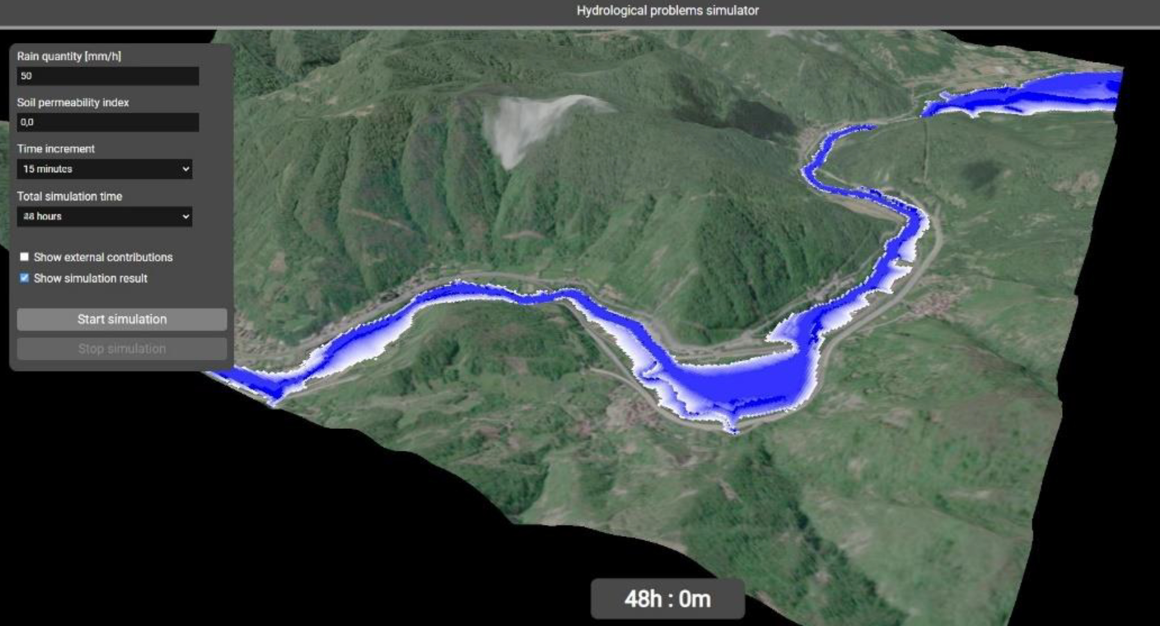
The execution of the simulation starts after the user has filled in the fields that determine the control parameters through the interface: it is possible to define the amount of water due to rainfall, expressed in mm/m2 per hour of rain, the time step between one frame and the next of the simulation, which can range from 15 to 120 minutes, the total time of the simulation duration, in the range of 6 to 48 hours. The last parameter to be selected will be a soil permeability index, which will affect the percentage of water that will be considered as absorbed by the soil and will therefore not increase the total volume of the overflow. This value can range from 0.0 (no permeability, found in rocky soils) to 1.0, (maximum permeability, which allows the soil to absorb the entire amount of water that falls, a condition that is obviously impossible in real cases).
Once this data has been collected, the platform will begin by first calculating a static map for external contributions. After that it will raise the geometries of the entire watercourse of the decided step, calculated as:
((rainfall amount + external contribution) * (1 - permeability index))
* (time step / total time).
An object representing the edge of the watercourse geometry (called fringe in platform) will then be generated by selecting all the cells that lie on the outer contour of the geometry. This will be the area that will be compared with the elevation, to be possibly expanded if the top of the cube of each of its cells is at a higher elevation than the direction in which it would like to expand.
In this way it will be possible to obtain an approximate simulation of the expansion of the volume of water as the amount of rain received increases, with an expansion stop in the case of slopes and areas with a higher ground elevation.
The water volumes displayed will also be colored in a graduation from white to deep blue as the height of the water volume in a given cell increases; to make it even clearer which areas are most affected by flooding.
In Figure 10 is the end result of a simulation that considers a time frame of 48 hours from the start of precipitation, assuming a constant amount of precipitation over time.
3.6. Simulation Platform
The platform uses the classic client - server scheme, thus allowing for use by several simultaneous users and publication on the web, possibly integrated within more extensive web portals that allow for different analyses of the territory for the mitigation of various types of risk (See Figure 11).
3.7. Back-End
The back-end of the application is realized in the Java language and is published on a dedicated Tomcat 9.0 application server (See Figure 12) [17].
This takes care of both serving the html, javascript and css files to the browser and providing the services for retrieving the geometry for the layers of the Openlayers map used on the front-end. The geometry data is stored within a PostgreSQL database with PostGIS extension (see).
For the connection between the Java code and the database, the JDBC (Java DataBase Connector) driver jar file was added to the application libraries. These drivers
allow the generic Connector, PreparedStatement and ResultSet classes of Java to be used with different types of databases including Oracle, MySQL, etc. In the case of the present study, the driver named postgresql-9.4-1101.jdbc41.jar (contained in the project’s WEB-INF/lib directory and linked in the application’s build path) allows use with PostgreSQL databases.
The format used for the exchange of geographic data between front-end and back-end is GeoJSON, a textual format that respects the specifications of the JSON format while incorporating the geographic information in a standard form directly readable by the Openlayers library.
For the back-end part, the project consists of two separate Java packages. In the first, database, there is the DataManager.java class, which takes care of instantiating connections to the PostgreSQL database and is solely responsible for query execution.
In the second package, servlet, are the classes that are responsible for serving content to the front-end in response to calls from the browser. The classes within it extend the HttpServlet class and respond to the URLs indicated by the @WebServlet annotation, as in the following example: @WebServlet(“/layers/getlayercorsiacqua”).
3.8. Front-End
The front-end, usable via all the latest browsers such as Google Chrome, Mozilla Firefox and Microsoft Edge, is realized in HTML, CSS and Javascript.
Some auxiliary libraries have been used for two- and three-dimensional visualization, and to facilitate access to certain types of data:
Openlayers.js: an open-source Javascript library designed to create interactive maps on the web. It provides an API that allows viewing, editing and managing geographical data from different sources, such as raster maps, vector maps and map services (OpenStreetMap, Google Maps or WMS services). It supports advanced features such as managing multiple layers, geolocalization, drawing geographical objects and interaction with GIS formats.
Three.js: for the creation of navigable three-dimensional screens, for the visualization of polygonal models. It also allows the application of textures and advanced effects, thanks to the potential of WebGL (Web Graphics Library).
Geotiff.js: for reading and managing data in geotiff format, with direct access to RAW image data.
Jquery: library of generic utilities that simplify many Javascript operations, including for example the handling of AJAX calls to the back-end [18].
The application is organized as a SPA (Single Page Application). This format is widely used for advanced web applications, and does not provide for the normal navigation between the various web pages as in a standard site, but manages any screen changes by means of javascript functions that regenerate the DOM, the object that takes care of maintaining a model of the current HTML document (See Figure 13).
The libraries are called up within the <head> section of the index.html file. Instead of importing them into the project, it was preferred to refer to the URLs of the repositories where they are made available [19]:
<!-- jquery --> src=https://code.jquery.com/jquery-3.4.1.min.js
<!-- Openlayers v.9.2.3 --> https://cdn.jsdelivr.net/npm/ol@v9.2.3/dist/ol.js https://cdn.jsdelivr.net/npm/ol@v9.2.3/ol.css
<!-- geotiff --> https://cdn.jsdelivr.net/npm/geotiff
https://cdn.jsdelivr.net/npm/geotiff@2.0.7/dist- browser/geotiff.js
<!-- three.js v. 0.164.1 -->
3.9. Three-Dimensional Rendering
The key part of the platform is the screen that runs the simulation and displays it in 3D. This choice is based on two main reasons: the first is that the three-dimensional X, Y, Z coordinates of the points of the terrain model are necessary for the execution of the simulation, as the expansion of the water volume is decided on the basis of the height of the surrounding terrain in relation to the height of the water; the second is the possibility for the user to rotate and zoom the model while the simulation is running, for a better evaluation of the effects of the flooding.
The capabilities of modern browsers allow the simulation to run in real time directly on the user’s terminal, not overloading the back-end server when running multiple instances of the platform.
The Three.js library provides, in the form of an API, the tools needed to create a 3D scene complete with polygonal objects, lighting effects, cameras and post-processing within a normal web page, exploiting the potential of the WebGL graphics libraries. Figure 14 shows the conceptual scheme of a Three.js scene.
Three.js is based on a number of software objects that encapsulate the main functionality of the software: The Renderer is the main object and is responsible for representing everything in a Scene on the screen, framing it as if the user were positioned at the point where the Camera is. This is modelled as a real camera with its own position, orientation and field of view (FOV) framing the scene (See Figure 15).
Within the Scene we find all the objects that make up the structure of the scene we are going to frame: the Mesh are the actual 3D objects. These are in turn composed of Geometry, the polygonal geometries that describe their appearance, and Material, the materials that define their color, light reflection properties, etc.
Materials may in turn refer to textures, raster images that are applied to the geometries, suitably extended or repeated to cover the entire model.
The scene will then be illuminated by Light objects, which may be of different types to simulate various types of light, such as spot, ambient, omnidirectional and so on.
One of the aspects to which attention must be paid for the correct visualisation of three-dimensional space is the co-ordinate system: although they always consist of the three axes X, Y, Z, some applications consider Z as the vertical axis, others Y. Three.js uses the latter convention, as shown in Figure 16.
Since in geographic systems longitude and latitude values are often traced back to X and Y co-ordinates, it would be more convenient, in the case of a geographic application, to use a reference system in which the Z axis corresponds to the vertical axis, representing the elevation of the terrain; the library allows the reference system to be changed via a simple function: THREE.Object3D.DefaultUp = new THREE.Vector3(0, 0, 1);
This creates a unit vector in the Z-direction and assigns it to the one that is considered ‘high’ (Up); in this way, the convention is restored to the desired condition.
3.10. Elevation Assignment
The terrain elevation comes from the DEM TINITALY 1.1 and is imported into the platform thanks to the use of the WCS services offered by the portal. These allow us to download a georeferenced GeoTIFF file directly to the browser, whose raw data can be used as the basis for the creation of a three-dimensional geometry that can be viewed using Three.js. The procedure begins with a call to the WCS services, as follows:
SERVICE=WCS &VERSION=1.0.0
&REQUEST=GetCoverage &FORMAT=GeoTIFF
&COVERAGE=TINItaly_1_1:tinitaly_dem
&BBOX= [coordinate iniziali e finali della zona di interesse] &CRS=EPSG:32632
&RESPONSE_CRS=EPSG:32632 &WIDTH=500
&HEIGHT=500
Among the various parameters passed to the caller, it is possible to note that the coordinate system used is 32632, which uses metres as the unit of measurement and thus facilitates the creation of the coordinates to be inserted in the BBOX (bounding box): for an area of 5km it will be sufficient to take the central point, in this case corresponding to the coordinates of the mouse at the click, and then add and subtract 2500 to obtain the start and end points of the GeoTIFF to be downloaded. In addition to this, the required image size is also specified, 500x500 pixels, corresponding precisely to an area of 5 x 5km, which corresponds to TINITALY’s definition of 10km per pixel.
The content of the response to this call is processed by the GeoTIFF.js libraries that allow the manipulation of the GeoTIFF raw data in the form of an arraybuffer, i.e., a sequence of bytes:
const arrayBuffer = event.target.response;
const tiff = await GeoTIFF.fromArrayBuffer(arrayBuffer); const image = await tiff.getImage();
const data = await image.readRasters();
renderData.demData = data [0];
In this code snippet, we create an object for the TIFF file by passing the contents of the response to GeoTIFF. From this object we extract the image, and in turn extract the raw data from it (remember that GeoTIFFs can contain multiple rasters within them, which is why the [0] element of the data array is selected, which in this case contains the data of the only image present).
This data is then saved within the renderData object, which is then passed on to the simulation.
Within the 3D visualisation, the elevation data will be realised by means of a plane with dimensions 5000 x 5000 metres, consisting of 499 vertices per side.
const geometry = new THREE.PlaneGeometry(5000, 5000, 499, 499);
The elevation values are stored within a one-dimensional array, as are the vertex positions in the Three.js plan. It will then suffice to create a loop with i ranging from 0 to the length of the array of positions, and assign the i- content of the array with the elevation data to each vertex:
position.setZ(i, data[i]);
The end result will be a mesh like the one shown in Figure 17:
In order to cast the simulation in as realistic an environment as possible, it is important to be able to intuitively visualize the area in which it takes place: for this purpose, having a ground texture showing satellite images of the area can make a strong contribution to the effectiveness of the tool. To achieve this, it will be necessary to have an image available, even one of arbitrary dimensions, to apply to the mesh representing the terrain.
First of all, a service was selected that could provide these images without cost, and without the need for API keys that could limit their use in the future: the choice fell on the ESRI services, which make available on their Tile Map Servers the layer called World Imagery, which contains the aerial and satellite maps of the entire planet. The service can be called up at the following URL:
Again, the OpenLayers libraries were used, generating a new map positioned outside the screen, using CSS properties:
position:fixed;left:0px;top:- 1030px;width:1024px;height:1024px;z-index:20).
After creating a layer capable of accessing the ESRI service, this is added to the map, which will have an extent equal to the bounding box of the area of interest.
When the rendering of the map is complete, the following function takes care of copying the content of the image into a raster, and passing it to the 3D simulation together with the rest of the basic data:
const mapCanvas = document.createElement(’canvas’); const size = map.getSize();
mapCanvas.width = size [0]; mapCanvas.height = size[1];
const mapContext = mapCanvas.getContext(’2d’); Array.prototype.forEach.call(
map.getViewport().querySelectorAll(‘.ol-layer canvas, canvas.ol-layer’), function (canvas) {
if (canvas.width > 0) {
const opacity = canvas.parentNode.style.opacity || canvas.style.opacity;
mapContext.globalAlpha = opacity === ‘‘ ? 1 : Number(opacity);
let matrix;
const transform = canvas.style.transform; if (transform) {
matrix=transform.match(/^matrix\( ([^\( ]*)\) $/)[1].split(‘,’)
.map(Number);
} else {
matrix = [parseFloat(canvas.style.width) / canvas.width, 0, 0,
parseFloat(canvas.style.height) / canvas.height, 0, 0];
}
CanvasRenderingContext2D.prototype.setTransform.apply(mapCo ntext, matrix);
const backgroundColor = canvas.parentNode.style.backgroundColor;
if (backgroundColor) { mapContext.fillStyle = backgroundColor;
mapContext.fillRect(0, 0, canvas.width, canvas.height);
}
mapContext.drawImage(canvas, 0, 0);
}},);
mapContext.globalAlpha = 1;
mapContext.setTransform(1, 0, 0, 1, 0, 0);
render3Dview(renderData.demData, renderData.alveoData, mapCanvas.toDataURL(“image/png”).replace(“image/png”, “image/octet-stream”));
The complete code for exporting a map as an image is available in the ‘Map Export’ example in the official OpenLayers documentation: https://openlayers.org/en/latest/examples/export-map.html
The data extracted in this way are passed to the 3D view creation function, and applied to the previously created plan using a standard Three.js material (See Figure 18):
var materialTerreno = new THREE.MeshPhongMaterial({ color: 0x55854f, specular: 0x555555, shininess: 20, flatShading: true
});
plane = new THREE.Mesh(geometry, materialTerreno); scene.add(plane);
Polygonal geometries from OpenStreetMap were chosen for the watercourses, imported into QGIS using the QuickOSM plug-in and subsequently saved to the PostgreSQL database serving the application. To allow their use within the 3D simulation, however, it is necessary to map these geometries onto the cells of the 5x5km area under consideration. To do this, the getFeaturesAtCoordinate() method of OpenLayers was used, which returns all features present at a certain coordinate passed in as input. Below is an extract of the function that performs this operation [20]:
const coordStart = ol.proj.transform([tiffData.bbox[0], tiffData.bbox[1]], ’EPSG:32632’, ’EPSG:3857’);
const coordEnd = ol.proj.transform([tiffData.bbox[2], tiffData.bbox[3]], ’EPSG:32632’, ’EPSG:3857’);
const startX = coordStart[0]; const startY = coordStart[1];
const stepX = (coordEnd[0] - coordStart[0]) / tiffData.width; const stepY = (coordEnd[1] - coordStart[1]) / tiffData.height; const arrayOut = [];
for (let x = 0; x < tiffData.width; x++) { arrayOut[x] = [];
for (let y = 0; y < tiffData.height; y++) {
let coords = [startX + (stepX * x), startY + (stepY * y)]; if
(layerCorsiAcqua.getSource().getFeaturesAtCoordinate(coords)
.length > 0) { arrayOut[x][y] = 1;
} else { arrayOut[x][y] = -1;
}}}
The function creates a grid of the same size as the elevation GeoTIFF, and scans this grid point by point: if a watercourse was found at that point, the corresponding element of the output array is assigned the value 1, otherwise the value -1. This array will then be inserted into the renderData object and passed to the function that is responsible for creating the 3D visualization.
Within this function, a parallelepiped geometry is created for each element of the two-dimensional array, with sides in the x- and y-direction 10m wide, and an initial height of 1m. This parallelepiped will be positioned at the height corresponding to the elevation plane for those coordinates, and the set of these parallelepipeds will constitute the initial riverbed of the watercourse on which the simulation will be performed. Below is the portion of the code that deals with generating the parallelepipeds:
const geometry = new THREE.BoxGeometry(10, 10, 1);
geometry.translate(x*10+offsetX, -(y*10+offsetY), val- baseZ+2);
const colors = new Uint8Array(72); for (let r = 0; r < 24; r++) { colors[r * 3] = 0;
colors[r * 3 + 1] = 0;
colors[r * 3 + 2] = 255;
}
const colorAttrib = new THREE.BufferAttribute(colors, 3, true);
geometry.setAttribute(’color’, colorAttrib); geometries.push(geometry);
All vertices in the geometry are assigned the colour blue (RGB 0, 0, 255). The array containing the vertex colours will have size 72, because it contains 3 integers (R, G, B) for the 24 vertices of the polygon (6 faces * 4 vertices each). When adding many polygons to the scene, a strong degradation in the performance of the application was noticed, and it was therefore decided to apply an improvement by merging all the different geometries into a single object:
const mergedGeometry = BufferGeometryUtils.mergeGeometries(geometries, false);
alveoMesh = new THREE.Mesh(mergedGeometry, materialAlveo); scene.add(alveoMesh);
This solution, although the number of vertices and faces is the same, allows for a considerable improvement in performance, because the drawCalls, the calls to the webGL services responsible for visualizing the scene, are reduced, since one is performed for each different object in the scene (See Figure 19).
3.11. Two-Dimensional Map
The two-dimensional map is realised using the OpenLayers libraries. As OpenLayers does not support the 32632 (UTM32) coordinate system by default, it was necessary to import the proj4 library into the project, which is responsible for extending the projections supported by OpenLayers, via the tag:
<script src=“https://cdn.jsdelivr.net/npm/proj4@2.11.0/dist/proj4.mi n.js”></script>
within the index.html file. At this point, using javascript, simply define the desired projection via the instruction:
proj4.defs(“EPSG:32632”, “+proj=utm +zone=32 +datum=WGS84
+units=m +no_defs +type=crs”);
ol.proj.proj4.register(proj4);
The map will consist of three layers that are always visible:
1. the OpenStreetMap base layer
2. the watercourse layer, polygonal
3.12. The Hydrographic Network Layer, Linear
First of all, the styles with which to represent the two vector layers must be defined, as follows:
const styleCorsiAcqua = new ol.style.Style({ stroke: new ol.style.Stroke({
color: “#5566ff”, width: 1
}),
fill: new ol.style.Fill({ color: “#5566ff”
})});
const styleReticoloIdrografico = new ol.style.Style({ stroke: new ol.style.Stroke({
color: “#0000ff”, width: 1
})});
At this point, it will be necessary to indicate the source of the data for both layers: in the case of the present project, the geometries are stored on the PostgreSQL database and supplied to the front end thanks to two servlets, which execute the queries and return the result in the form of GeoJSON, a format ready to be consumed by the OpenLayers source object (the example is given for the ‘Watercourses’ layer, the process is equivalent for the hydrographic network):
const vectorSource1 = new ol.source.Vector({ loader: function (extent) {
var source = this;
$.ajax({
url: ’layers/getlayercorsiacqua’, context: document.body
}).done(function (response) {
source.addFeatures((new ol.format.GeoJSON()).readFeatures(response));
});},
strategy: ol.loadingstrategy.all, projection: ’EPSG:32632’
});
Once the data source has been populated, it is finally possible to instantiate an object of type layer:
layerCorsiAcqua = new ol.layer.VectorImage({ source: vectorSource1,
name: “Corsi d’acqua”, style: styleCorsiAcqua, zIndex: 5
});
The layer type chosen is VectorImage, which combines the flexibility and speed of vector layers with the possibility of generating cache images typical of raster vectors, for reuse in the case of tiles already previously shown on screen.
As far as the base layer is concerned, things are even simpler, since OpenLayers natively provides an object of type source.OSM that takes data directly from the OpenStreetMap services.
const OSMbasemap = new ol.layer.Tile({ source: new ol.source.OSM(),
});
In this case, the layer is of type Tile, as it shows a mosaic of pre-generated images. The map is thus complete, and we can instantiate it by inserting all the layers created previously:
olMap = new ol.Map({
target: ’map’, layers: [
OSMbasemap, layerCorsiAcqua, layerReticoloIdrografico
],
view: new ol.View({
center: [981941, 5496717],
zoom: 9,
}),
projection: ’EPSG:32632’,
});
Events such as clicking on a map and selecting features on certain layers can then be recorded, in order to perform the relevant operations required for the platform to function.
3.13. User Interface
The application consists of two different screens. The initial screen is a classic two-dimensional map showing the watercourses, the hydrographic network and the boundaries of the area of interest. The second is a 3D screen, which can be viewed after selecting an area on which to run the simulation, where it is possible to set parameters and launch the actual simulation.
The two-dimensional map view of the territory is the screen that is displayed when accessing the application URL (See Figure 20) [21].
The interface is very simple: the main element is the map, freely navigable and clickable. In addition to the zoom buttons on the left, which are provided directly by the OpenLayers API, there are two buttons for displaying the DEM in a 5km area around the clicked point, and the button for the 3D view, which is activated when the DEM is displayed (See Figure 21).
On the map there are, in addition to the OpenStreetMap base layer, two layers: the first displays the watercourses downloaded from OpenStreetMap in vector form, while the second represents the hydrographic network downloaded from the geoportal of the Liguria region.
Clicking on a given point on the map will search for information on the latter layer. If elements are found, these will be colored in yellow and a pop-up window will open containing various information on the selected section of the grid (See Figure 22).
The reported data are:
- The name of the watercourse
- The Strahler order
- The indicative specific surface area, expressed in square meters
- The indicative surface area of the underlying basin, expressed in square meters
- Whether the watercourse is hydraulically surveyed or not
When clicking on the ‘View DEM’ button you will be asked to click on a point on the map, and once a point has been selected the TINITALY WCS service will be called up which returns the GeoTIFF of the elevation for a 5x5km area around the selected coordinates. The GeoTIFF, in addition to being scanned to send elevation data to the simulation, is also displayed on the map for a better understanding of the area over which it will operate (See Figure 23).
At this point, the ‘3D View’ button will be made active and, if there are watercourses within the area, you can move on to the actual simulation.
3.14. Three-Dimensional Visualization Map
Upon clicking the ‘3D View’ button, you will be redirected to the relevant page, where the 3D terrain model, the riverbed of the watercourse in blue color, and all user interface elements allowing interaction with the simulation will be displayed (See Figure 24).
In particular, thanks to the panel on the left of the screen it will be possible to select (See Figure 25)
- The amount of rain falling in the area in an hour (mm/h)
- The soil permeability index, from 0.0 (completely impermeable) to 1.0 (completely permeable)
- The time increment for each ‘frame’ of the simulation
- The total simulation time
In addition to these input parameters, there are two checkboxes: the first allows you to display, instead of the textured terrain, the map of external contributions, with a graduation from green to red depending on the contribution each cell makes to the volume of water. The second, on the other hand, allows the display of the simulation result to be activated/deactivated after the simulation is completed, as can be seen in Figure 26:
This option allows a better comparison between the initial and final situation, and a better understanding of which areas have been flooded compared to the initial riverbed. Below the two checkboxes are the two main buttons: The first allows the simulation to be started, while the second allows it to be interrupted if intermediate effects with respect to the selected time horizon are to be assessed. During the execution of the simulation, the time relative to the current frame is indicated by the timer at the bottom of the screen.
4. Conclusions and Future Work
This research activity describes the design and implementation of a tool for the simulation of hydrological risk in the event of rainfall-related flooding of a watercourse, showing the results through a three-dimensional representation of the affected water mass and the surrounding terrain. The simulation is based on the morphology of the terrain adjacent to the affected watercourse bed, taking elevation into consideration to determine the direction of expansion of the water mass.
A distinctive aspect of the platform is its extreme speed in the resolution of simulations, which also allows the tool to be used in real time. This means that during the occurrence of a meteorological event, the platform can be used to monitor the evolution of the situation and predict the effects of any persistence of the phenomenon over time. This real-time forecasting capability is crucial for making quick and informed decisions, thus reducing reaction times and improving emergency management on the ground, with a potential positive impact on the safety of the population and the protection of infrastructure.
A very important feature of the research work performed is the possibility of running simulations on any device with an internet connection, without the need for specific hardware or particularly high resources. This makes the platform accessible from laptops, tablets or even smartphones, offering considerable operational flexibility for users. In this way, the platform can be used not only by emergency operators at the various sites of the agencies involved, but also by those who are directly in the field, perhaps during monitoring and control operations in areas at risk.
This feature makes it possible to obtain up-to-date information in real time, even in emergency situations, where quick access to data and the ability to develop up-to-date scenarios can make a difference in managing operations. Mobile use allows, for example, technicians and operators in the field to monitor the evolution of weather and hydrological conditions directly on site, to quickly share simulation results with coordination centers, and to make decisions based on concrete and up-to-date data without having to worry about the availability of powerful workstations or computing servers. Moreover, this accessibility reduces operational costs related to the purchase and maintenance of specific equipment, making the platform a particularly cost-effective solution for public authorities, civil protection, and land management organizations, even in resource-limited settings.
For the purpose of this research activity, it was decided to limit the platform’s area of use to the Liguria region only. For use in cases of real floods, however, it is obviously necessary to use it to launch simulations over a wider area, possibly including the entire extent of the country.
The platform has therefore been designed in such a way that it can be easily extended to the entire Italian territory: the Tinitaly portal makes raster elevation maps available for the entire country, and the WCS service made available already allows the download of geoTIFFs of the Italian territory from the coordinates entered. Polygonal data containing watercourse geometries are also available on OpenStreetMap and can be downloaded, e.g., through the open-source QuickOSM plug-in used, to be imported into the application’s database.
Most of the damage caused by flood events is the inundation and related damage to buildings located near the riverbed of the affected rivers or watercourses, either with structural damage to the buildings, or with non-structural damage to the contents and any inhabitants or occupants in the case of industrial/commercial buildings. For this reason, a useful addition for damage mitigation purposes would be the three-dimensional geometries of the buildings in the areas affected by the flood: based on their height and the height reached by the water, it would be possible to estimate the amount of damage that could possibly result, and to prepare for their evacuation in the event that there could be danger to inhabitants or occupants. Again, for a good part of the Italian built environment, OpenStreetMap makes available the height data of the various buildings in addition to their polygonal representation on a map. Through the union of these two data, it will be possible to extrude the geometries in elevation to obtain a fairly realistic three-dimensional representation of the buildings to be integrated in the simulation. This would allow an approximate assessment of which elevation, and thus for example which floor of the building, would be reached by the water level in the event of a flood.
A further aspect of the simulation that could be worked on is the refinement of the analysis performed: for example, having a point or area description of the permeability of the terrain, one could use this data to determine the amount of water absorbed by the soil instead of relying on a static index entered by the user that remains static for the entire area under consideration; one could also use elevation maps at a higher resolution to model the area, and thus also the riverbed, more accurately; the simulation would also be more accurate as one would be modelling a greater number of cells, each with a smaller size and thus with greater fidelity than in the real case.
It would also be possible to exploit less approximate algorithms for the simulation of surface runoff, i.e., the movement of rainwater on the slopes that will flow into the riverbed. In any case, a compromise will have to be found between the fidelity of the simulation and the speed of execution, since an excessive complexity of the analyses carried out could compromise the platform’s usability in real time, defeating its purpose and leading to the use of more complex software that exploits dynamic fluid simulations to predict the movement of the mass of water involved in the outflow from the riverbed.
The platform has been designed with a modular architecture, which allows this type of change and integration to be made quickly and easily within the simulation flow. This feature provides great flexibility, allowing new functionality to be added or existing algorithms to be updated without having to redesign the entire system.
The modularity of the platform is based on a clear separation between the different analysis phases that are performed on the model, such as the calculation of slopes, the calculation of the surface runoff map, the calculation of the amount absorbed by the soil, and finally the simulation of scenarios. Each phase operates independently, but is designed to integrate with the others, facilitating the replacement or updating of individual modules without compromising the overall operation.
This modular structure not only facilitates the technological upgrading of the platform, but also allows it to be adapted to the specific needs of different territorial or operational contexts. For example, the platform can be customized to address particular hydrogeological hazards in a specific region or to meet the needs of different entities operating in the territory. Thanks to this flexibility, the platform can stay abreast of scientific and technological advances, guaranteeing a simulation capability that is always up-to-date and responsive to real needs on the ground.
Author Contributions
Conceptualization, Mauro Mazzei; methodology, Mauro Mazzei; software, Davide Quaroni; validation, Mauro Mazzei, Davide Quaroni; formal analysis, Mauro Mazzei; data curation, Mauro Mazzei and Davide Quaroni; writing—review and editing, Mauro Mazzei and Davide Quaroni; supervision, Mauro Mazzei. All authors have read and agreed to the published version of the manuscript.
Funding
This research received no external funding.
Data Availability Statement
The source of the data of the maps are the ISPRA (Institute for Environmental and Environmental Research) the INGV Institute (National Institute of Geophysics and Volcanology) with which it provides used for the project is TINITALY/1.1.
Acknowledgments
The authors thank Istituto Superiore per la protezione e la Ricerca Ambientale, l’Istituto Nazionale di Geofisica e Vulcanologia, Research Center as a source of documentation necessary for the conduct of this paper.
Conflicts of Interest
The authors declare no conflict of interest.
References
- Rapporto sulle condizioni di pericolosità da alluvione in Italia e indicatori di rischio associati. Available online: https://www.isprambiente.gov.it/files2021/pubblicazioni/rapporti/rapporto_alluvioni_ispra_353_16_11_2021_rev2.pdf (accessed on September 2024).
- Available online: https://www.khronos.org/webgl/ (accessed on September 2024).
- Threejs.org documentation, Getting Started. Available online: https://threejs.org/docs/index.html#manual/en/introduction/Creating-a-scene (accessed on September 2024).
- Openlayers API. Available online: https://openlayers.org/en/latest/apidoc/ (accessed on September 2024).
- OpenStreetMap. Available online: https://www.openstreetmap.org/ (accessed on September 2024).
- Tarquini, S.; Isola, I.; Favalli, M.; Battistini, A.; Dotta, G. TINITALY, a digital elevation model of Italy with a 10 meters cell size (Version 1.1). Istituto Nazionale di Geofisica e Vulcanologia (INGV). 2023. [Google Scholar] [CrossRef]
- ESRI portal. Available online: https://www.esri.com/en-us/home (accessed on September 2024).
- Dissesto idrogeologico in Italia: pericolosità e indicatori di rischio. Edizione 2021. ISPRA, Rapporti 356/2021.
- European Commission, Joint Research Centre; De Groeve, T.; Revilla-Romero, B.; Pappenberger, F.; Salamon, P.; Thiemig, V.; Thielen-del Pozo, J.; Hirpa, F. The Benefit of Continental Flood Early Warning Systems to Reduce the Impact of Flood Disasters; European Union Publications Office: Luxembourg, 2016. [Google Scholar]
- Tazen, F.; Diarra, A.; Kabore, R.F.W.; Ibrahim, B.; Bologo/Traoré, M.; Traoré, K.; Karambiri, H. Trends in flood events and their relationship to extreme rainfall in an urban area of Sahelian West Africa: The case study of Ouagadougou, Burkina Faso. J. Flood Risk Manag. 2019, 12, e12507. [Google Scholar] [CrossRef]
- Aich, V.; Liersch, S.; Vetter, T.; Andersson, J.; Müller, E.; Hattermann, F. Climate or Land Use?—Attribution of Changes in River Flooding in the Sahel Zone. Water 2015, 7, 2796–2820. [Google Scholar] [CrossRef]
- Massazza, G.; Bacci, M.; Descroix, L.; Ibrahim, M.H.; Fiorillo, E.; Katiellou, G.L.; Panthou, G.; Pezzoli, A.; Rosso, M.; Sauzedde, E.; et al. Recent Changes in Hydroclimatic Patterns over Medium Niger River Basins at the Origin of the 2020 Flood in Niamey (Niger). Water 2021, 13, 1659. [Google Scholar] [CrossRef]
- World Bank, GFDRR. The State of Hydrological Services in Developing Countries. 2018. Available online: https://www.gfdrr.org/sites/default/files/publication/state-of-hydrological-services_web.pdf (accessed on 20 December 2021).
- Giuliani, G.; Nativi, S.; Obregon, A.; Beniston, M.; Lehmann, A. Spatially enabling the Global Framework for Climate Services: Reviewing geospatial solutions to efficiently share and integrate climate data & information. Clim. Serv. 2017, 8, 44–58. [Google Scholar]
- OGC. OpenGIS® Web Services Architecture Description, Version: 0.1.0; Whiteside, A., Ed.; OGC 05-042r2; Open Geospatial Consortium: Wayland, MA, USA, 2005; p. 22. Available online: https://www.ogc.org/docs/bp (accessed on 20 December 2021).
- Copernicus, Operational Review of the Record Flood in Niamey, Niger. Sentinel Vision, EVT-719, 27 August 2020. Available online: https://www.sentinelvision.eu/gallery/html/fab25b31f6064dcf9caf84cc693051af (accessed on 10 January 2022).
- Capodiferro, C.; De Maria, M.; Mazzei, M.; Spreafico, M.; V. Bik, O.; Palma, A.L.; V. Solovyeva, A. Cultural Itineraries Generated by Smart Data on the Web. ISPRS Int. J. Geo-Inf. 2024, 13, 47. [Google Scholar] [CrossRef]
- Mazzei, M.; Quaroni, D. Development of a 3D WebGIS Application for the Visualization of Seismic Risk on Infrastructural Work. ISPRS Int. J. Geo-Inf. 2022, 11, 22. [Google Scholar] [CrossRef]
- Formica, A.; Mazzei, M.; Pourabbas, E.; Rafanelli, M. Approximate Query Answering Based on Topological Neighborhood and Semantic Similarity in OpenStreetMap. IEEE Access 2020, 8, 87011–87030. [Google Scholar] [CrossRef]
- Mazzei, M.; Di Guida, S. Spatial Data Warehouse and Spatial OLAP in Indoor/Outdoor Cultural Environments. In Computational Science and Its Applications – ICCSA 2018; Gervasi, O., et al., Eds.; Lecture Notes in Computer Science; Springer: Cham, Switzerland, 2018; Volume 10962. [Google Scholar] [CrossRef]
- Geoportale della Regione Liguria. Available online: https://geoportal.regione.liguria.it/ (accessed on September 2024).
Figure 1.
River in flood and river in low.
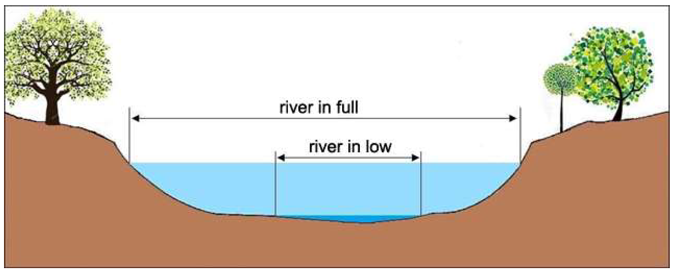
Figure 2.
Floodable areas per high flood hazard scenario.
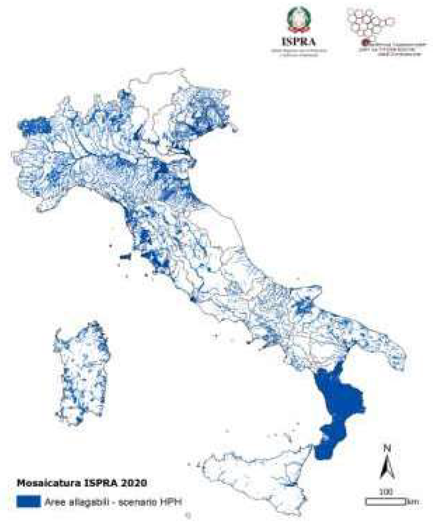
Figure 3.
Resident population in flood-prone areas for the three flood probability scenarios, national level - ISPRA Mosaic, 2020.
Figure 3.
Resident population in flood-prone areas for the three flood probability scenarios, national level - ISPRA Mosaic, 2020.
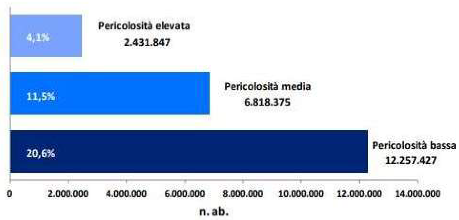
Figure 4.
Map of the Lambro, Seveso, Olona basin.
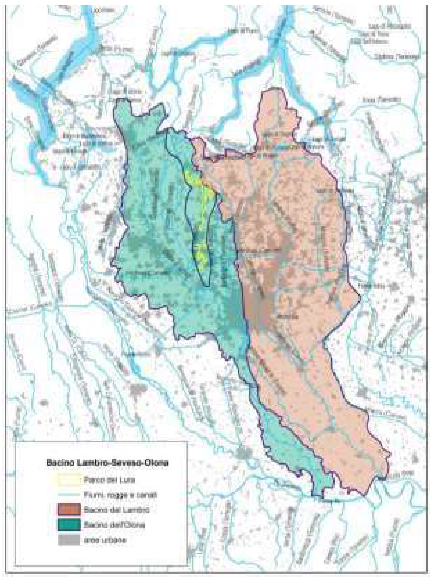
Figure 5.
Strahler sorting.
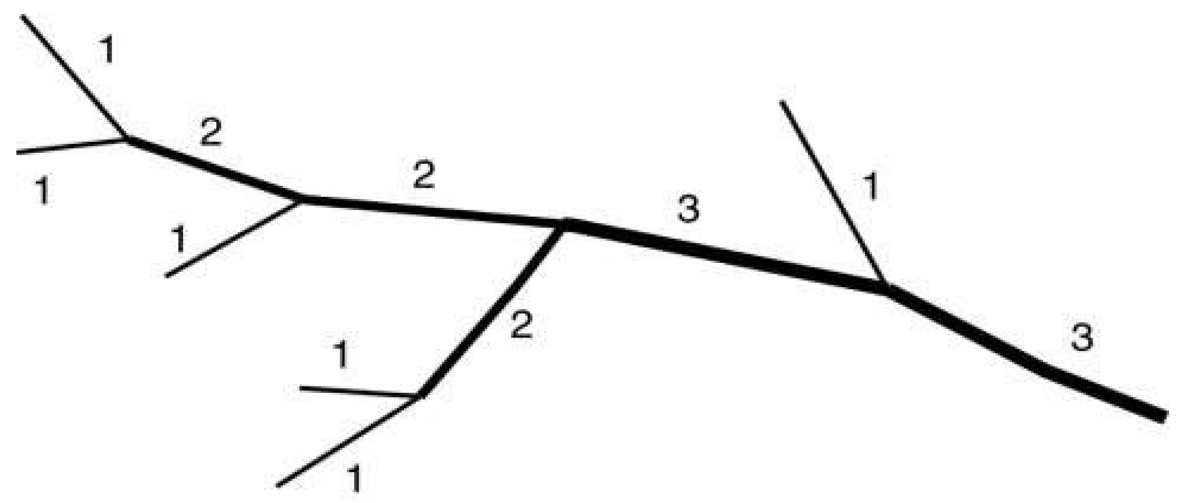
Figure 6.
DEM Tinitaly/1.1.
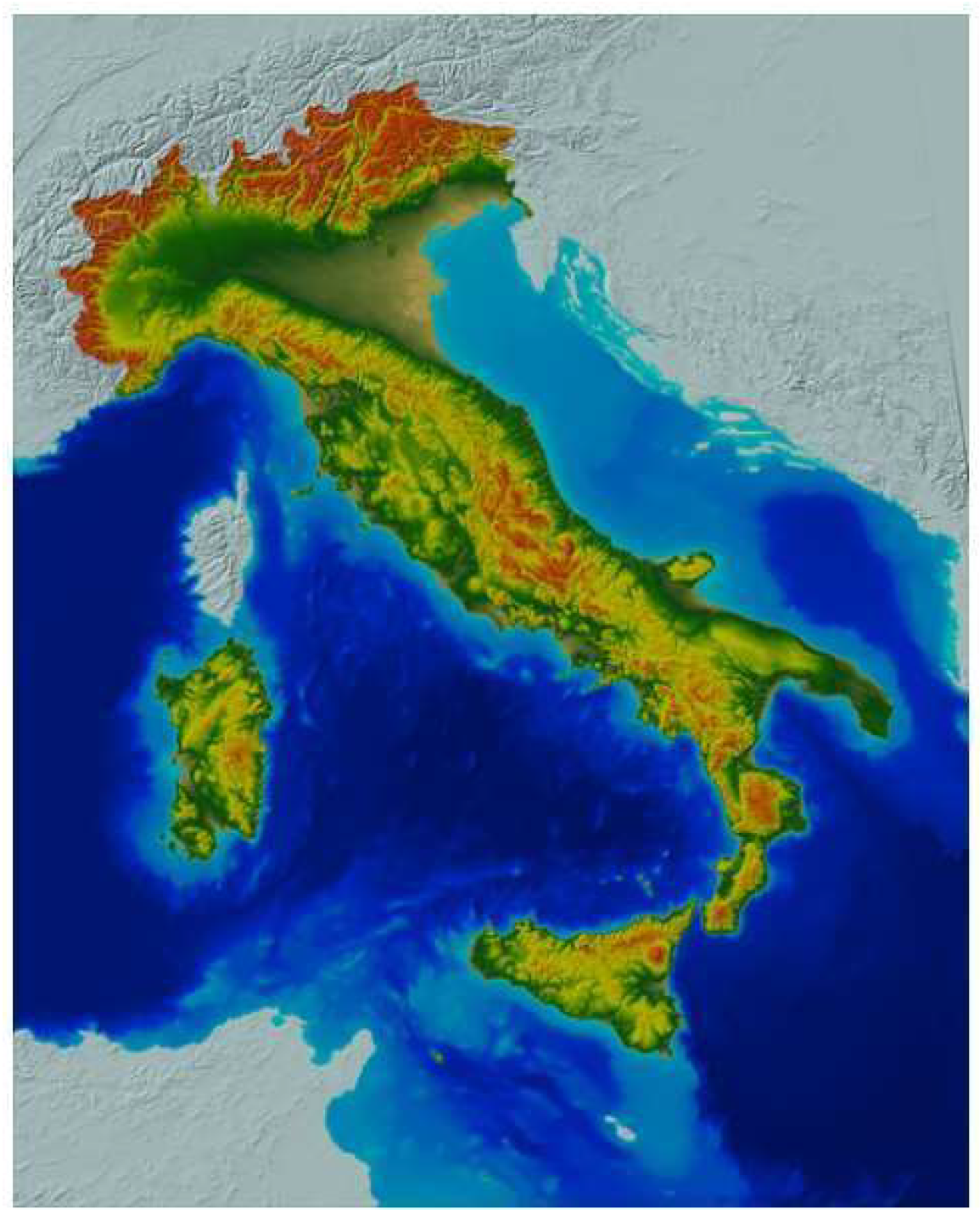
Figure 7.
Watercourse layer and DEM portion within the platform.
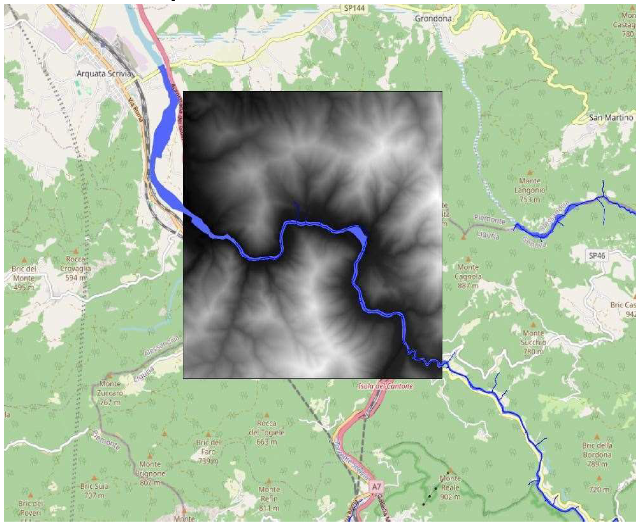
Figure 8.
Example of runoff based on relative slope.
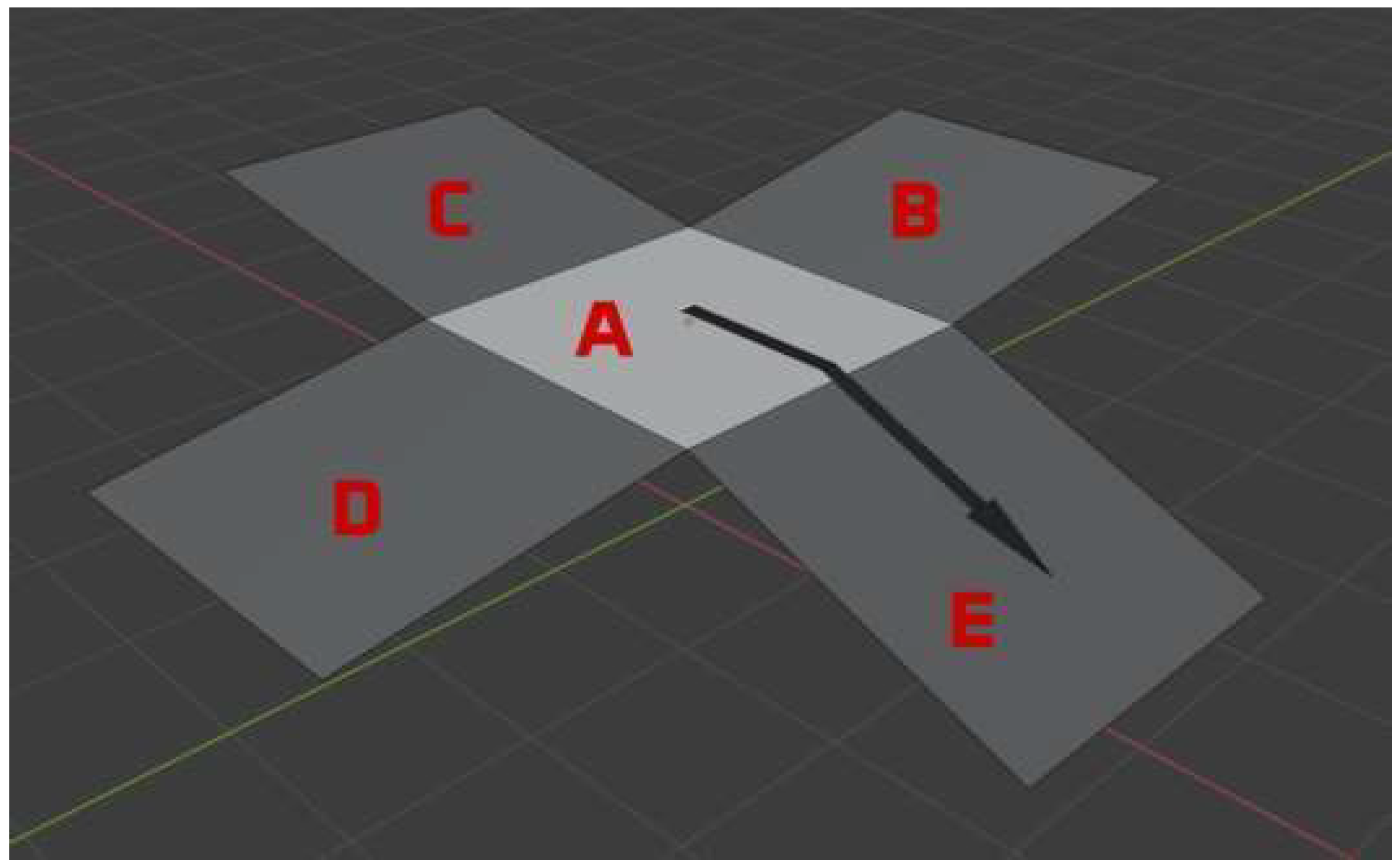
Figure 9.
Static map of external contributions based on surface runoff.
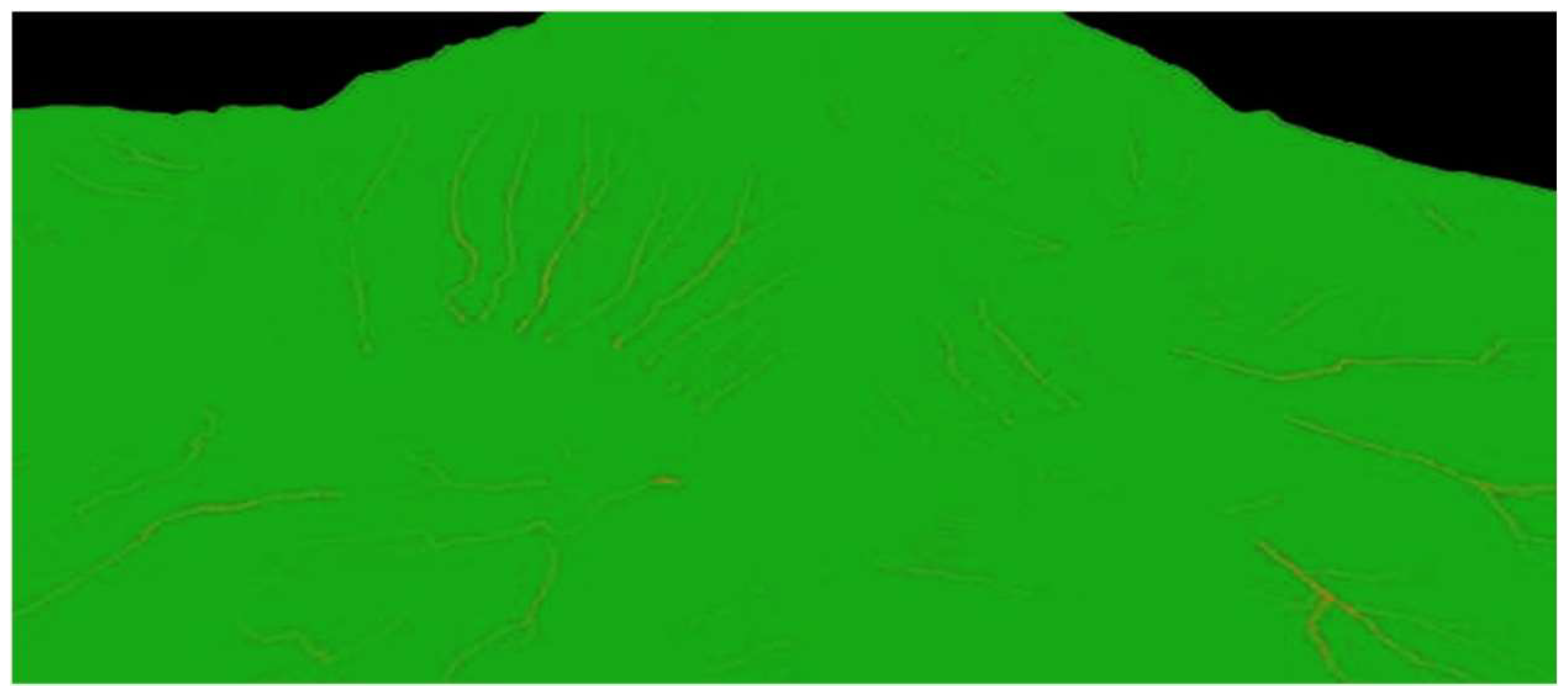
Figure 10.
Final result of a simulation.
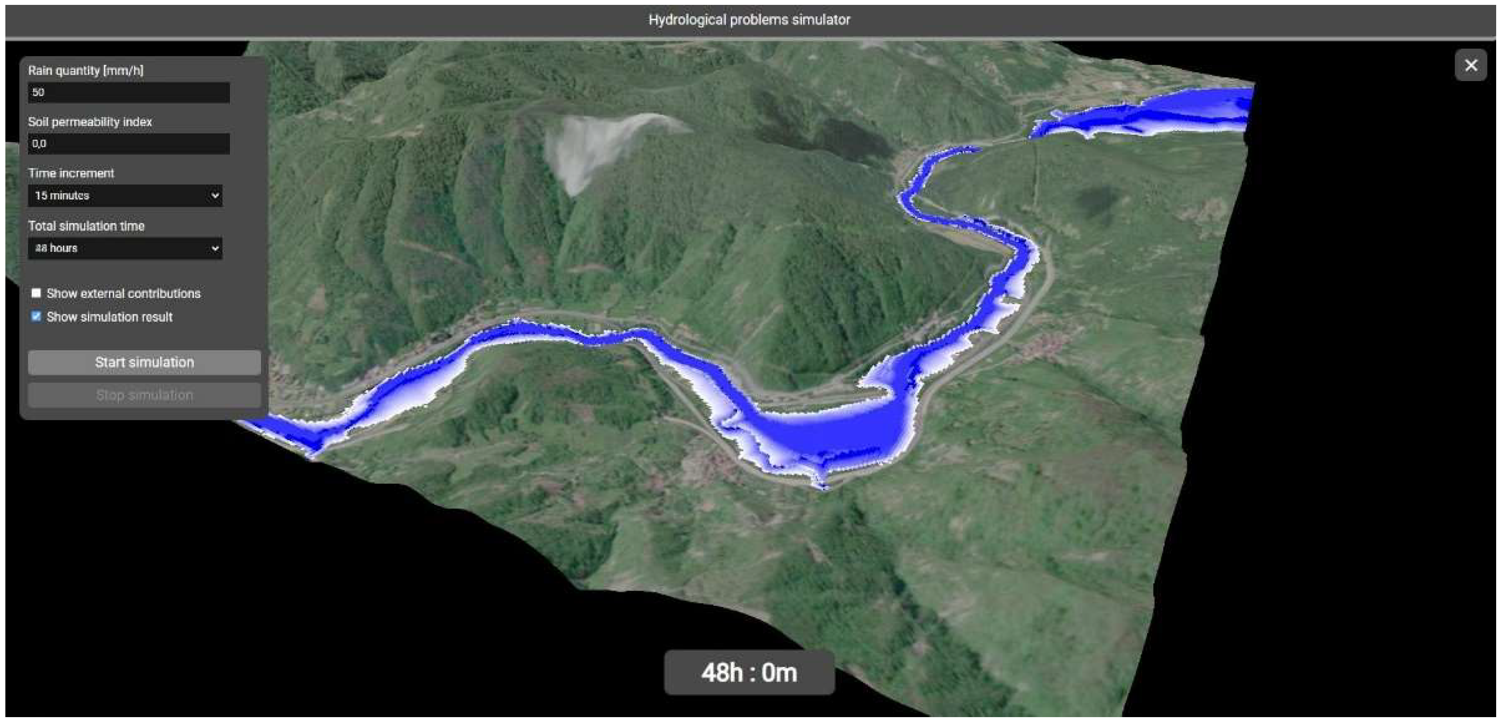
Figure 11.
System architecture.
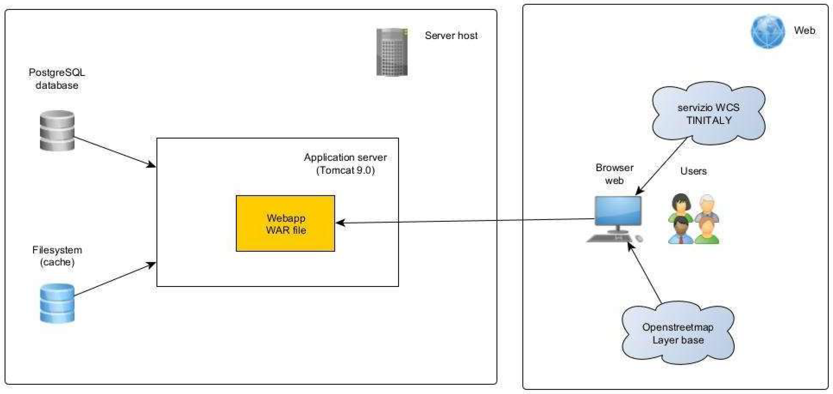
Figure 12.
Project file structure - back-end.
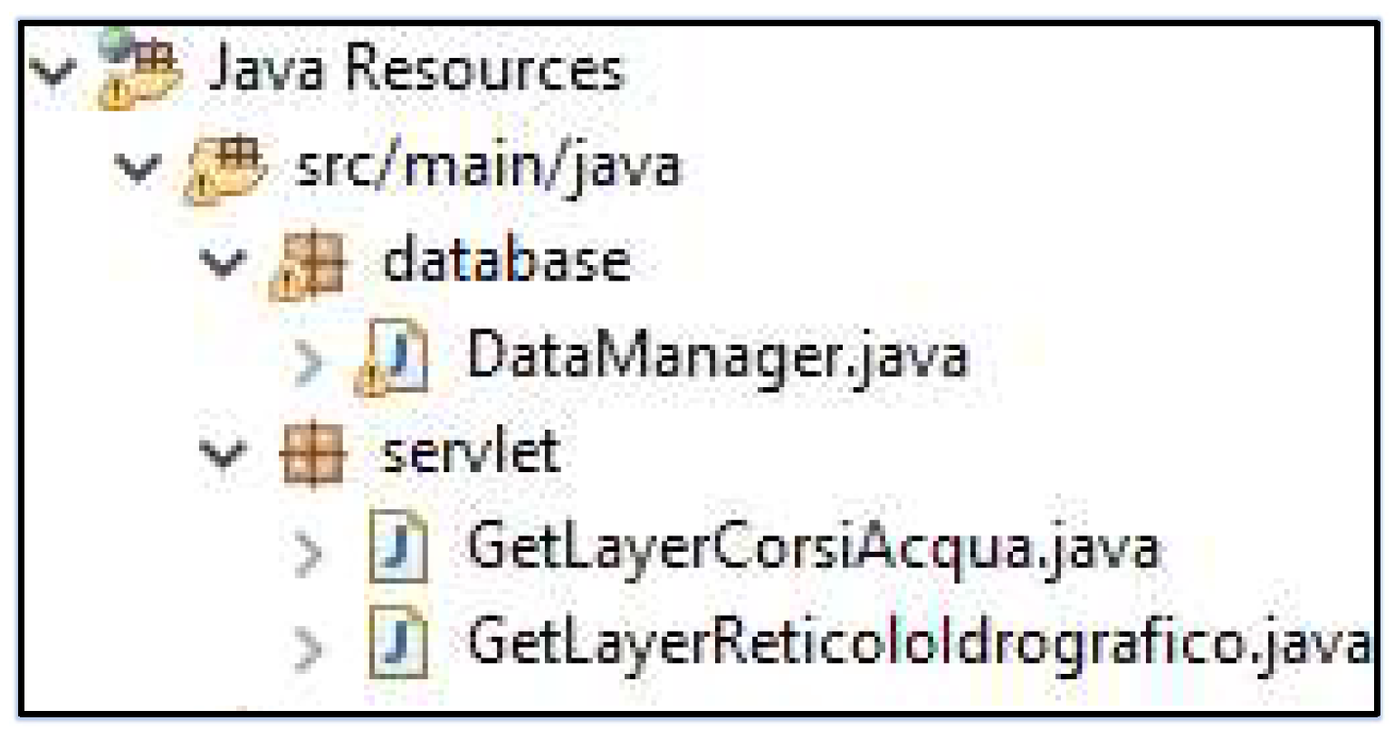
Figure 13.
Project file structure - front-end.
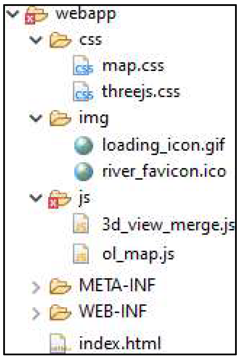
Figure 14.
Conceptual diagram of a scene.
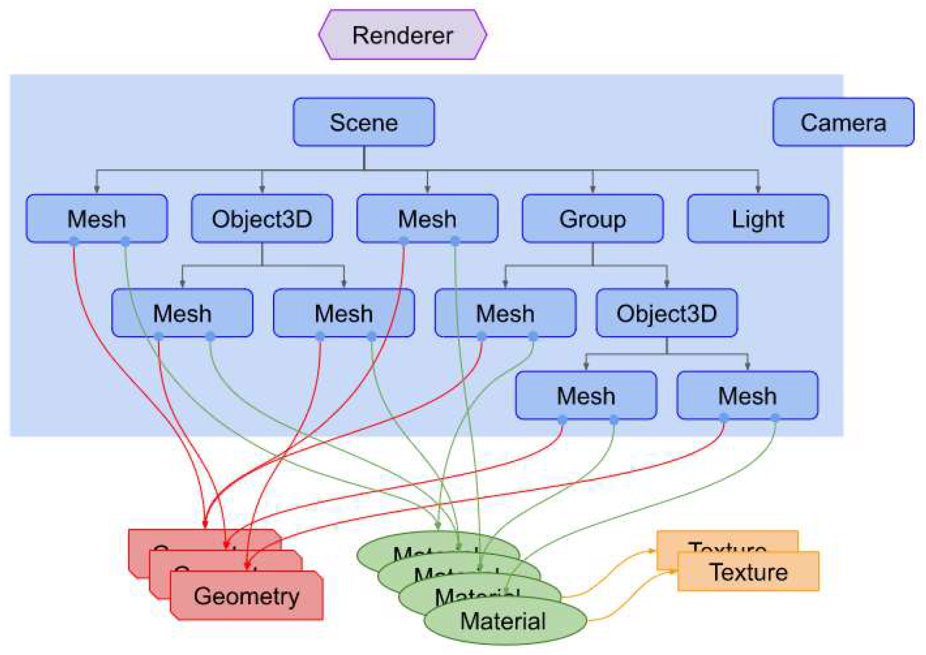
Figure 15.
Camera-related concepts.
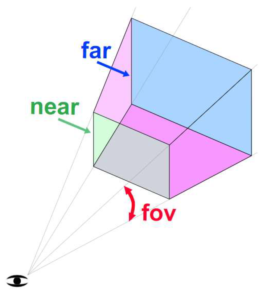
Figure 16.
Axis direction in Three.js.
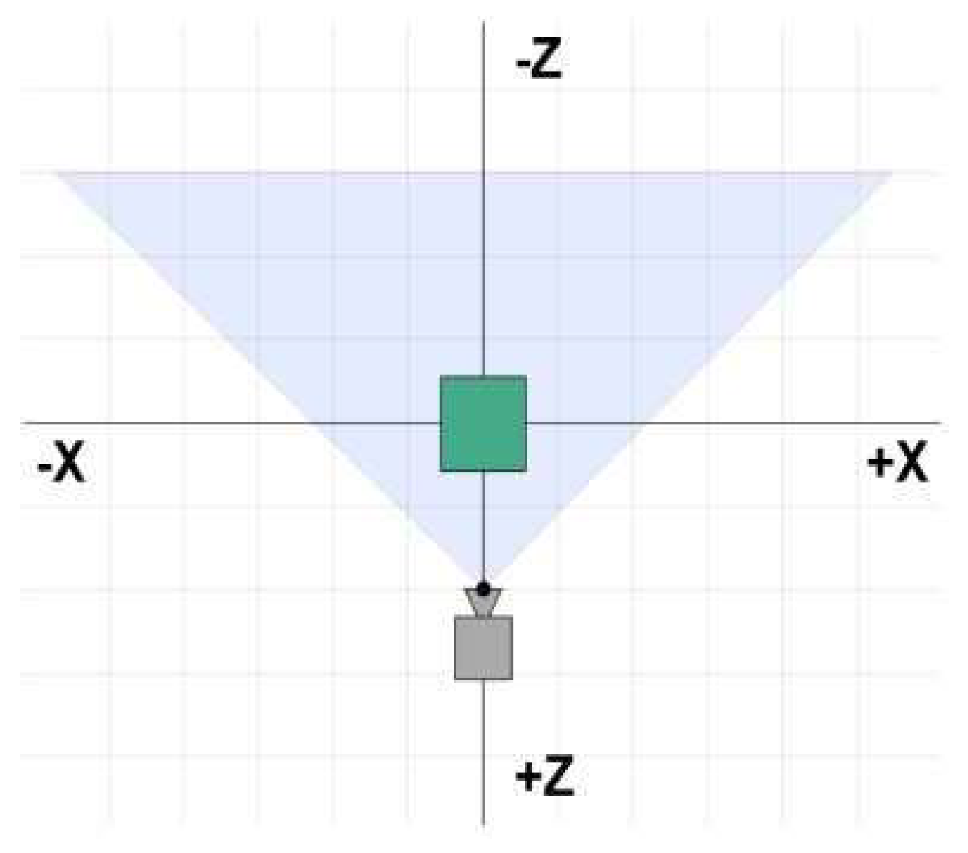
Figure 17.
3D representation of the plane with elevation.
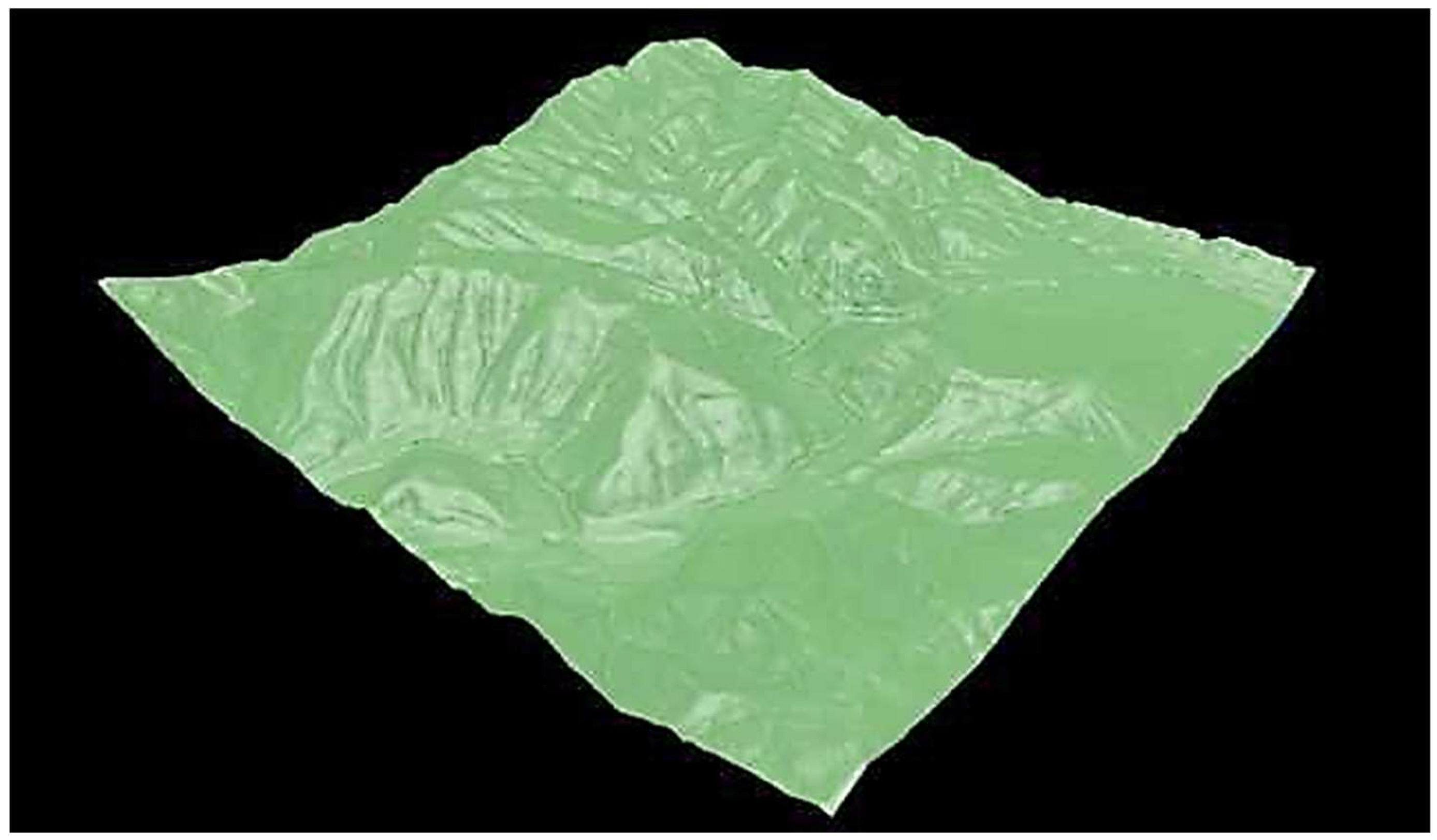
Figure 18.
Texture applied to 3D plane.
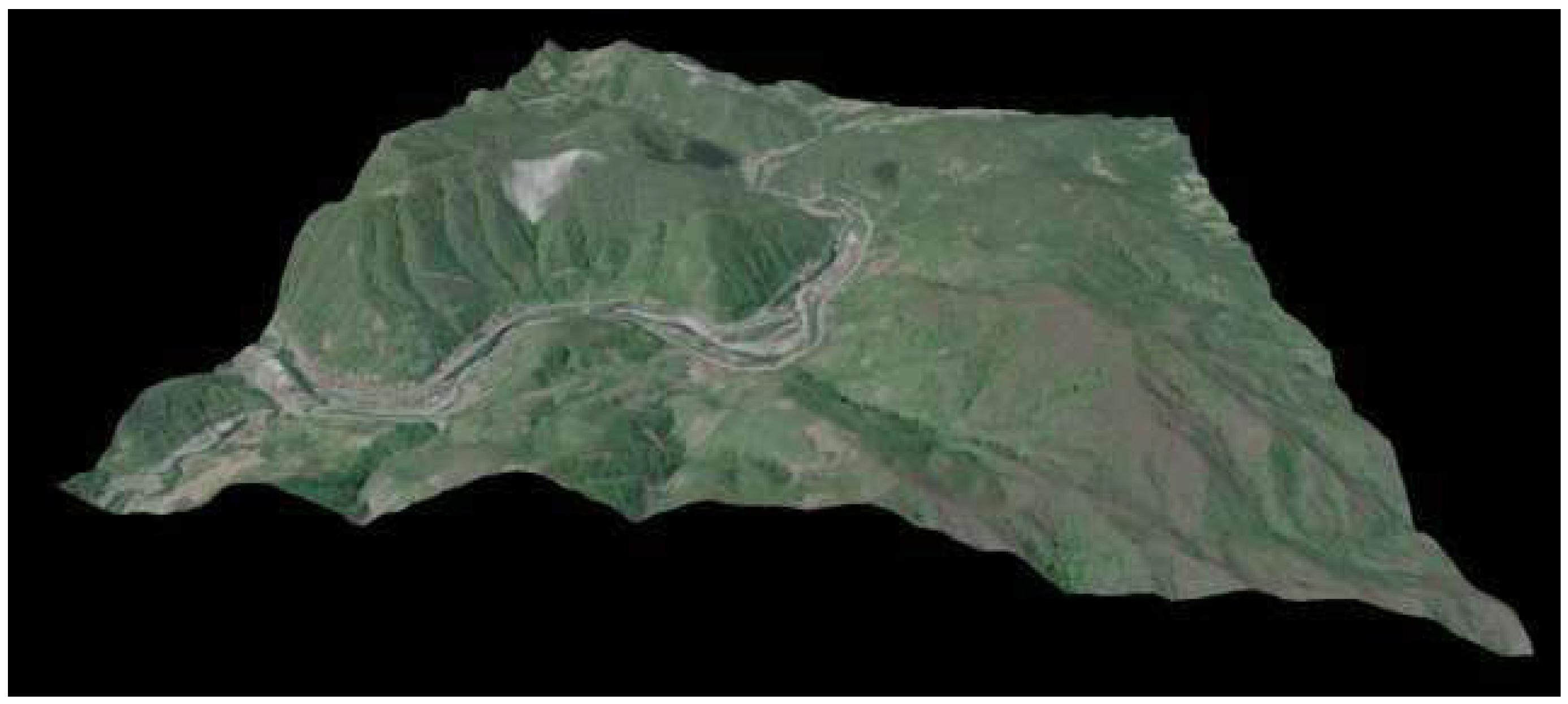
Figure 19.
3D visualization of the riverbed.
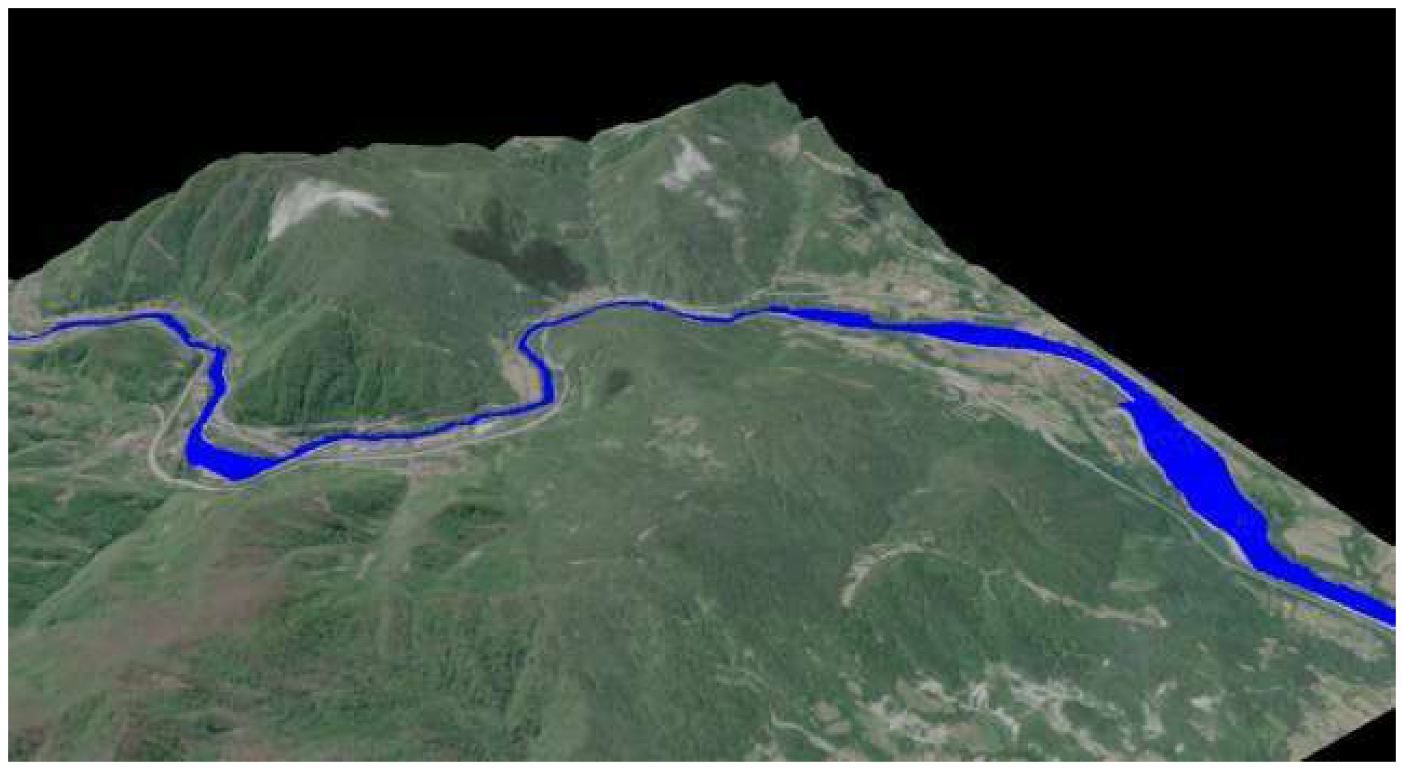
Figure 20.
User interface - two-dimensional display.
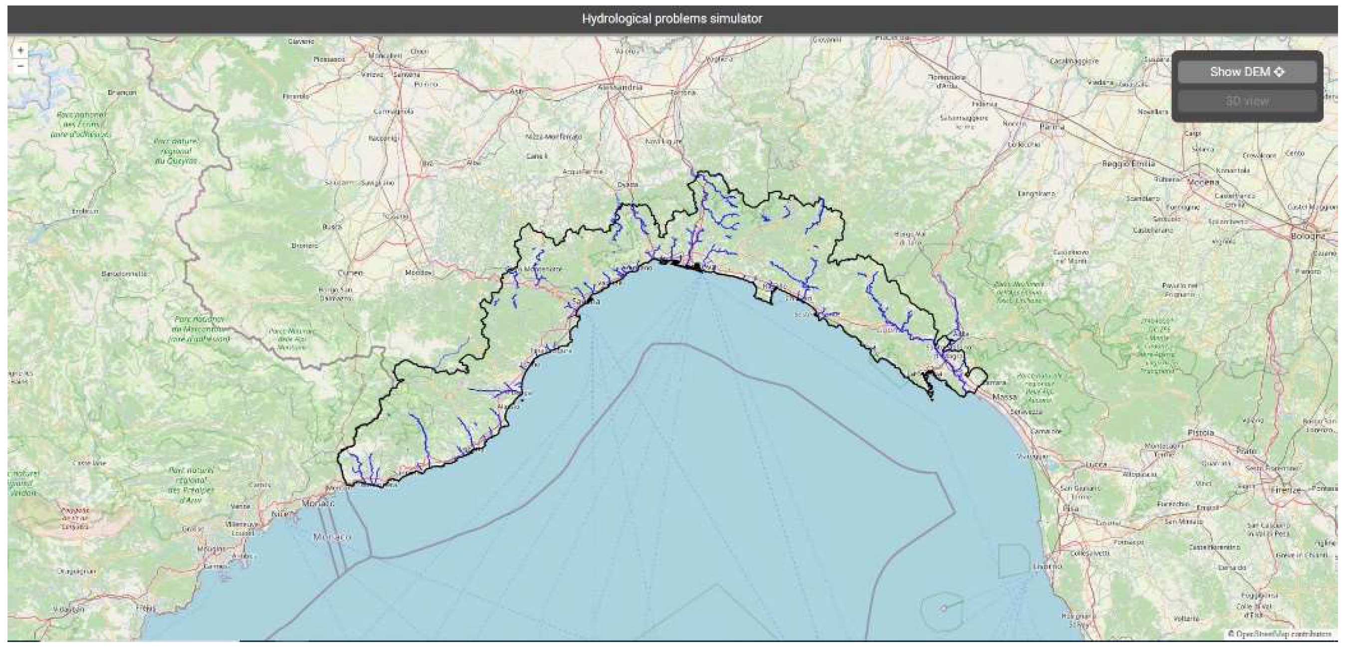
Figure 21.
Button panel.
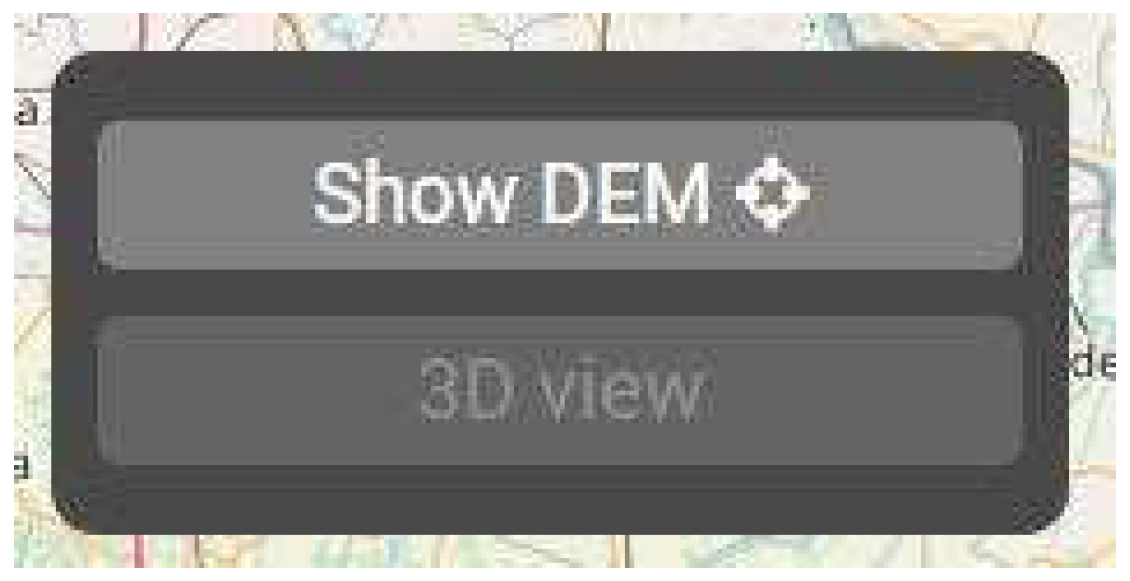
Figure 22.
Pop-up with details of the selected feature.
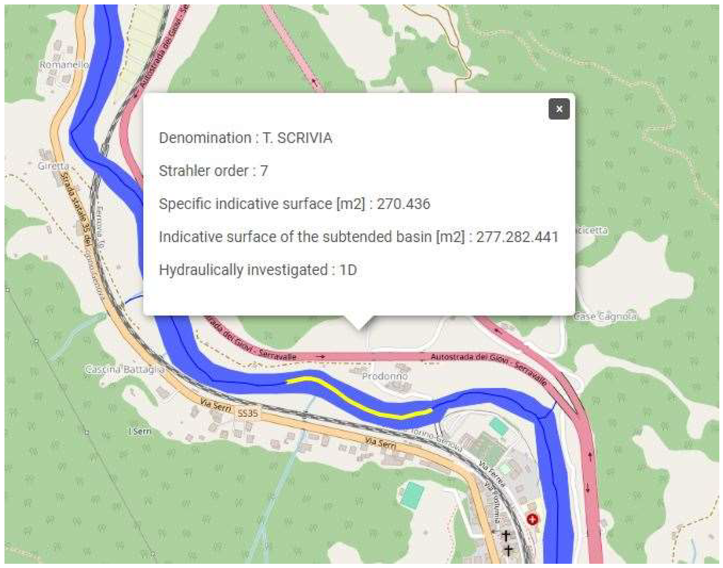
Figure 23.
Visualization of the DEM portion.
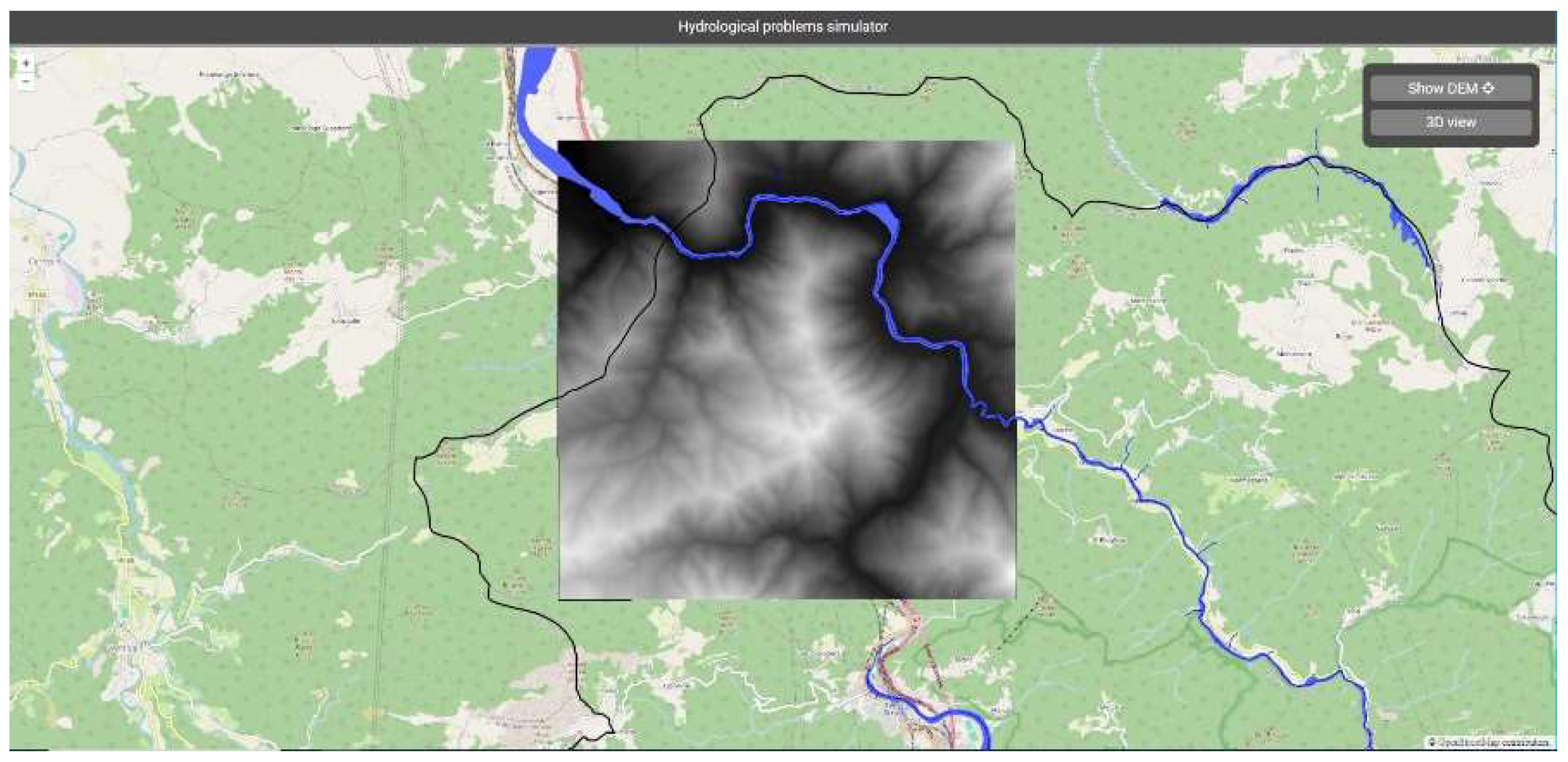
Figure 24.
User interface - three-dimensional visualization.
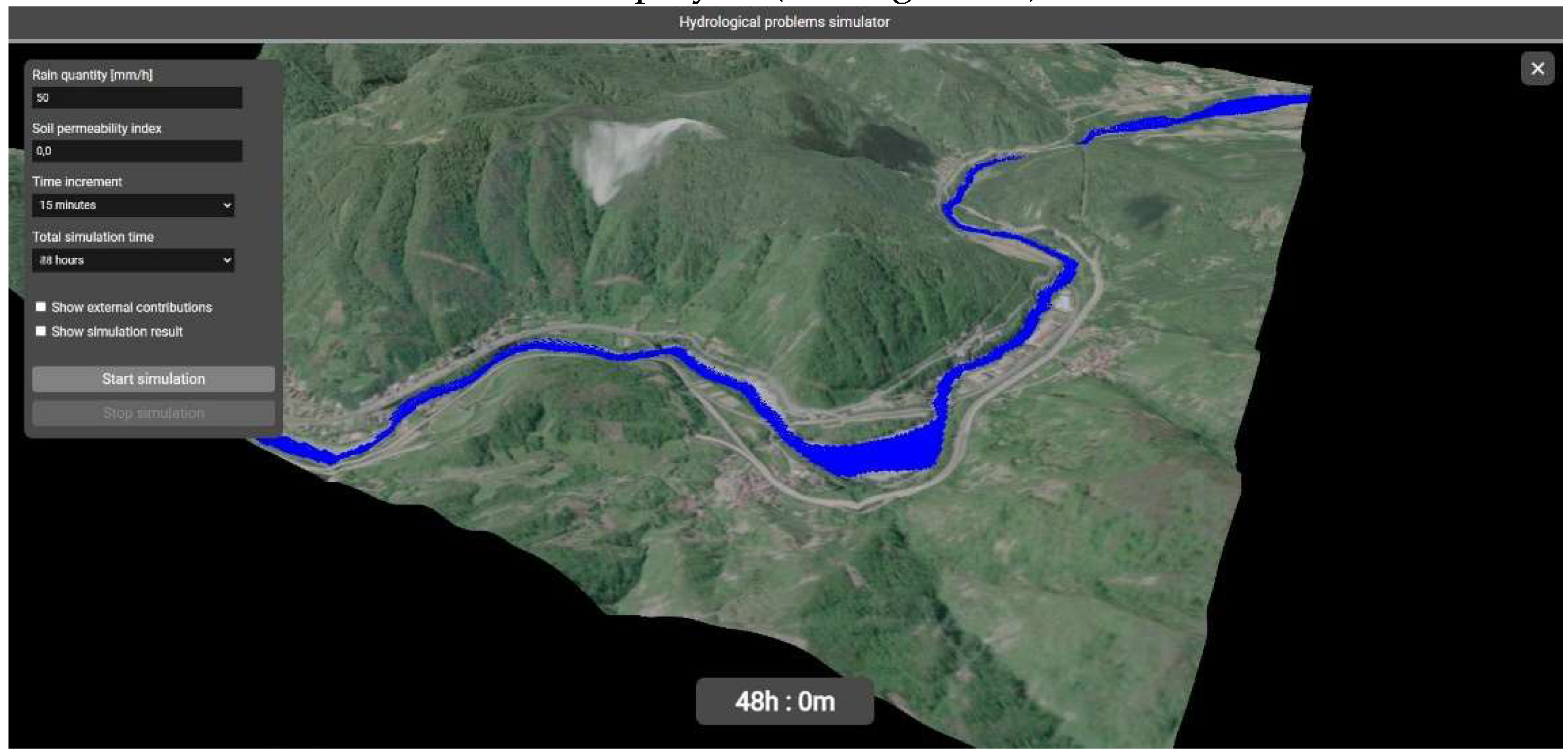
Figure 25.
Simulation control panel.
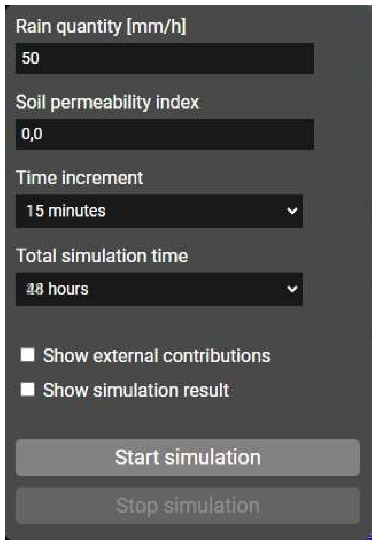
Figure 26.
Comparison of the situation at the beginning and end of the simulation.
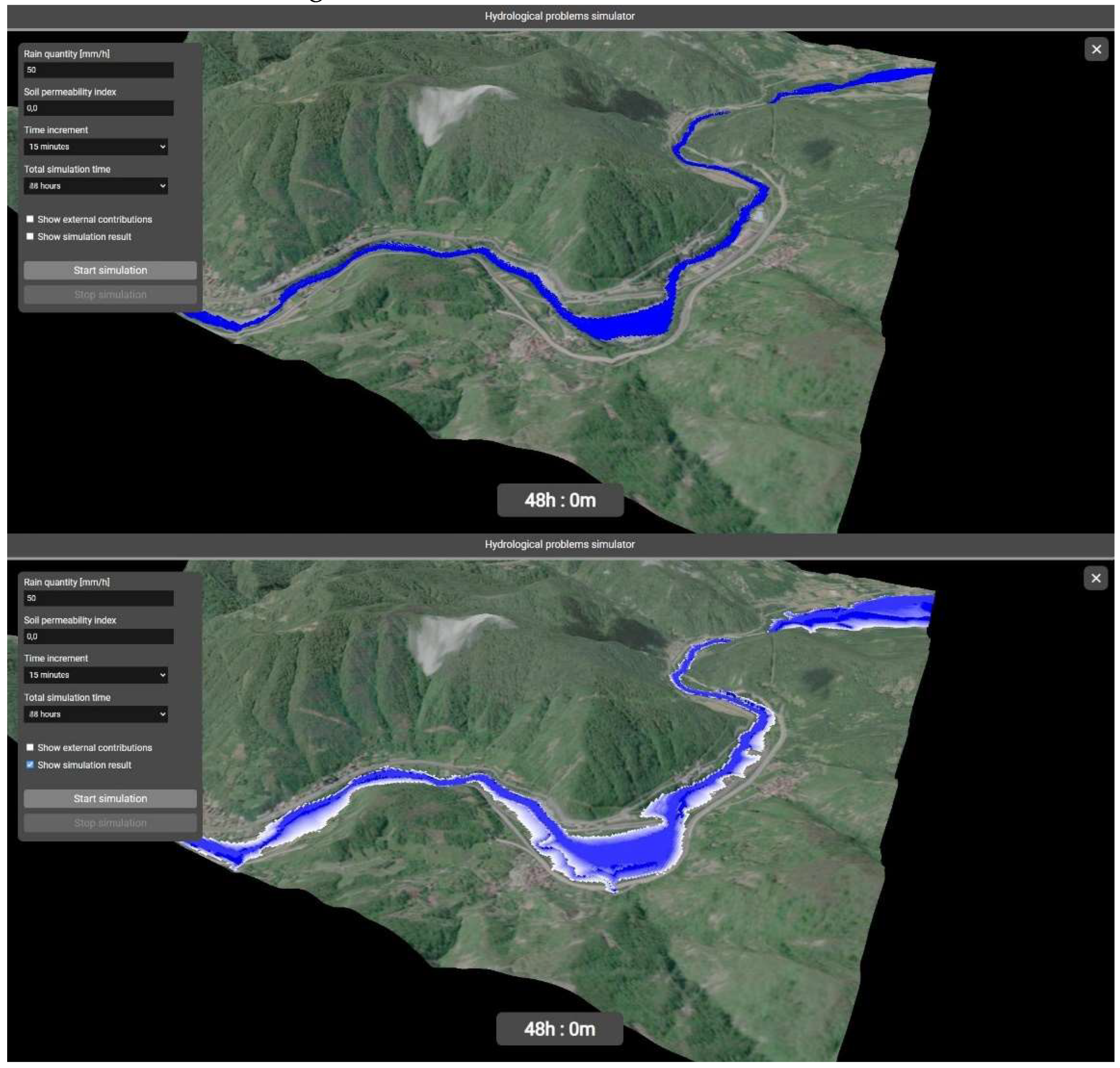
Disclaimer/Publisher’s Note: The statements, opinions and data contained in all publications are solely those of the individual author(s) and contributor(s) and not of MDPI and/or the editor(s). MDPI and/or the editor(s) disclaim responsibility for any injury to people or property resulting from any ideas, methods, instructions or products referred to in the content. |
© 2024 by the authors. Licensee MDPI, Basel, Switzerland. This article is an open access article distributed under the terms and conditions of the Creative Commons Attribution (CC BY) license (http://creativecommons.org/licenses/by/4.0/).
Copyright: This open access article is published under a Creative Commons CC BY 4.0 license, which permit the free download, distribution, and reuse, provided that the author and preprint are cited in any reuse.


