
Submitted:
17 December 2024
Posted:
19 December 2024
You are already at the latest version
Abstract
This paper is concerned with the derivation of the Edgeworth expansion for the standardized and the studentized version of the kernel-based estimator of the expectile. Inverting the expansion allows us to construct accurate confidence intervals for the expectile. The theoretical asymptotic results are applied for moderate sample sizes. The methodology is illustrated with an application in risk management in finance for the estimation and accurate confidence interval construction for the coherent risk measure expectile-VaR.
Keywords:
Nonparametric Statistics
; Expectile
; Kernel
; Smoothing
; Risk
; Edgeworth Expansion
1. Introduction
Quantile-based inference has been a long-standing interest in the financial industry and risk assessment. A few applications worth mentioning include: the widely used risk measure VaR (value at risk) is a tantamount quantile; coherent risk measures typically represent transformations of quantiles; quantile regression has been used as a tool for portfolio investment decisions.
For a continuous random variable X with a cumulative distribution function density function and the th quantile is defined as
Given a sample from the simplest estimator of is the sample quantile. Under mild conditions, it is asymptotically normal, but its asymptotic variance is large, particularly in the tails. Hence, it behaves poorly for small sample sizes, and alternative estimators are needed. The kernel quantile estimator
is an obvious choice. Here is the inverse of the empirical distribution function, is a suitably chosen kernel, and is a bandwidth. Conditions on bandwidth and kernel must be imposed to ensure consistency, asymptotic normality, and higher-order accuracy of
This type of research has been of considerable interest also to the authors of the current paper. We derived in [12] higher order expansion for the standardised kernel quantile estimator thus extending long-standing flagship results of [6,7]. Our expansion is non-trivial because of the influence of the bandwidth that makes the balance between bias and variance delicate.
We then derived in [13] an Edgeworth expansion for the studentized version of the kernel quantile estimator (where the variance of the estimator is estimated using the jackknife method). Precisely this result is needed for practical applications since the variance is rarely known in practice. The inversion of the Egdeworth expansion delivered a uniform improvement in coverage accuracy compared to the inversion of the asymptotically normal approximation. Our results are applicable to improve inference for quantiles when the sample sizes are small to moderate. This situation often occurs in practice. For example, if monthly loss data is used in risk analysis, then for 10 years, the accumulated data would amount to 120 observations. There are only about 250 trading days on the stock market within a year.
After the global financial crisis, the activities of the bank regulators were directed toward proposing measures of risk that could be an alternative to the VaR. The coherency requirement for a risk measure in finance was first formulated in the seminal paper [1] and has been widely used since then. We note that VaR is not a coherent risk measure mainly because it does not satisfy the subadditivity property. The AVaR (average value at risk) does satisfy the subadditivity and turns out to be a coherent risk measure. It was considered around 2009 as an alternative risk measure by the Basel Committee of Banking Supervision. Meanwhile, academic research on the properties of risk measures continued. The elicitability property was pointed out as another essential requirement in [8]. The latter property is an important requirement associated with effective backtesting. It then turned out that expectiles “have it all" as they are simultaneously coherent and elicitable. Moreover, it was shown (see, for example, [17]) that expectiles are the only law-invariant risk measures that are simultaneously coherent and elicitable.
It was natural for us then to turn to expectiles and to propose methods for improved inference about expectiles for small to moderate sample sizes. The current paper suggests such a methodology and illustrates its effectiveness. The paper is organized as follows. In the next Section 2 we introduce some notations, definitions, and auxiliary statements we need in the sequel. Section 3 presents our main results about the Edgeworth expansion of the asymptotic distribution of the estimator. This section is subdivided into three subsections. The first subsection deals with the standardized kernel-based expectile estimator. The second subsection discusses the related results for the studentized kernel-based expectile estimator. While the first subsection is of theoretical interest mainly, the results of the second subsection can be directly applied to derive more accurate confidence intervals for the expectile of the population for small to moderate samples. The third subsection discusses a Cornish-Fisher-type approximation for the quantile of the kernel-based expectile estimator. The application for accurate confidence interval construction presents the main purpose of our methodology. Its efficiency is illustrated numerically in the next Section 4. Section 5 summarizes our findings. Technical results and proofs of the main statements of the paper are postponed to the Appendix.
2. Materials and Methods
From a methodological standpoint, is an L-estimator: it can be written as a weighted sum of the order statistics
Consider a random variable Using the notations Newey and Powel introduced in [15] the expectile as the minimizer of the asymmetric quadratic loss
and we realize that its empirical variant can also be represented as an L-statistic. When we get which means that the expectiles can be interpreted as an asymmetric generalization of the mean. In addition, it has been shown in several papers (see for example [2]) that the so-called expectile-VaR ( is a coherent risk measure when as it satisfies the four coherency axioms from [1]. Any value of can be used in the definition of the expectile but for the reason mentioned in the previous sentence, we will assume that in the theoretical developments of this paper.
The asymptotic properties of L-statistics are usually discussed by first decomposing them into an U-statistic plus a small-order remainder term and then applying asymptotic theory of the U-statistic. For starters, the L statistic is written as where is the empirical distribution function and the score function does not involve For the presentation (2), however, such a decomposition is impossible as the “score function” becomes a delta function in the limit. Therefore, a dedicated approach is needed. For the case of quantiles, details about such an approach are given in [13]. Our current paper shows how the issue can be resolved in the case of expectiles. The main tools in our derivations are some large deviation results on U-statistics from [14].
Remark.
We mention in passing that in the paper [10], it is shown that expectiles of a distribution F are in a one-to-one correspondence to quantiles of another distribution G that is related to F by an explicit formula. It might be tempting to use this relation to utilize our results from [13] in the construction of confidence intervals for the expectiles of We have examined this option and realize that the correspondence is quite complicated involving functionals of F that need to be estimated by the data. It turns out that proceeding in this way is not an option to construct precise confidence intervals for the expectiles. Hence, our way to proceed is to deal directly from the very beginning with the definition of the expectile of
We start with some initial notations, definitions, and auxiliary statements.
We consider a sample of n independently and identically distributed random variables with density and cumulative distribution functions respectively.
Let us define
where is an indicator function. Looking at the original definition (3) we can define the (true theoretical) expectile as a solution to the Equation
Using the relation we realize that the defining Equation (4) leads to the same solution as the defining Equation (2) in [2] or the defining Equation (2) in [9].
As discussed in [9], the -expectile satisfies the Equation
Using integration by parts, we have the following proposition.
Proposition 1.
Assume that . Then we have
where and Thus an estimator of the expectile is given by a solution of the equation
where is the sample mean and is the empirical distribution function.
Holzmann and Klar in [9] have proved a uniform consistency and asymptotic normality of . In this paper, we study the higher-order asymptotic properties of the expectile estimator. To study the higher-order asymptotics, we use a kernel-type estimator of the distribution function , instead of .
Let us define kernel estimators of the density and distribution function
where is a kernel function and is an integral of . We assume that
and Here h is a bandwidth where . Hereafter we assume that the bandwidth .
As in the case of quantile estimation, we are using a kernel-smoothed estimator of the cumulative distribution function in the construction of the expectile estimator. The reason for switching to the kernel-smoothed version of the empirical distribution function in the definition of our expectile estimator is that only for this version is it possible to show the validity of the Edgeworth expansion. As discussed in detail in [13], if we use a kernel estimator with an informed choice of bandwidth and a suitable kernel, then the resulting expectile estimator can be easily studentized; the Edgeworth expansion up to order for the studentized version will be derived and the theoretical quantities involved in the expansion can be shown to be easily estimated. In addition, a Cornish-Fisher inversion can be used to construct confidence intervals for the expectile (which is the main goal of the inference in this paper). The resulting confidence intervals are more precise than the intervals obtained via inversion of the normal approximation and can be used to improve the coverage accuracy for moderate sample sizes.
Hence from now on we will discuss the higher order asymptotic properties of the estimator of that satisfies
Let us define
Then similarly to Proposition 1, we have the following Proposition.
Proposition 2.
If the kernel function satisfies the condition (a1), the kernel expectile estimator is given by the solution of the equation
For our further discussion we define the following quantities.
Definition 1.
Note that holds and that and denote the biases of the kernel estimators of and
Since we intend to discuss the Edgeworth expansion with a residual term , we will obtain the asymptotic representation with residual term where
as . When we obtain the Edgeworth expansion until the order , it follows from Esseen’s smoothing lemma that we can ignore the terms of order .
Similarly to the notation, we will also be using the notation that follows the definition
Note that we can also ignore the terms when we discuss the Edgeworth expansion with residual term .
3. Results
3.1. Edgeworth Expansion for the Standardized Expectile
In this subsection, we will get an asymptotic representation of the standardized expectile and its Edgeworth expansion. This expansion is of theoretical interest mainly as the constant C and the normalizing quantity involved depend on parameters of the unknown population distribution. Later, in SubSection 3.2 we will formulate the related but more practicable expansions of the studentized expectile. They do not depend on unknown population parameters and can also be inverted to deliver accurate asymptotic confidence intervals for the expectile.
We assume that the following conditions hold:
Theorem 1.
We assume the conditions hold. Further, assume that , the derivatives and are bounded, and . Then:
(1) For the standardized expectile estimator, we have
where
(2)The asymptotic variance of is equal to where
, and
(3) The Edgeworth expansion is given by
where
and
Remark 1
It follows from the results of Holzmann and Klar in [9] that
Comparing with the result of Corollary 4 on p. 2359 in [9] we realize that, as expected, the first-order approximations of the asymptotic variances of the kernel-smoothed expectile estimator in our paper and of the empirical distribution-based estimator discussed in [9] coincide.
It is easy to see that
and this relation can be used to write down the formula for in (9) in an alternative way.
The proof of the above Theorem will be presented in the Appendix. It relies heavily on some large deviations results for U-statistics that we summarized in Lemma A1 (whose formulations and proof are also postponed to the Appendix). Using the results of the latter Lemma, we can obtain the evaluation of the order of the asymptotic approximations and expansions of the differences (also to be presented in Lemma A2 in the Appendix). Combining the evaluations from Lemma A2 essentially guarantees the asymptotic representation in the standardized case given in Theorem 1.
3.2. Edgeworth Expansion for the Studentized Expectile
As pointed out by many papers, the Edgeworth expansion of the studentized estimator is more important than the expansion of the standardized estimator. In addition, it is the studentized version that could be inverted in practical settings to deliver confidence intervals for the unknown expectile. In order to get the asymptotic representation of the studentized estimator, we need to construct suitable estimators and . is given in (Definition 1) already. Next we proceed to get an estimator of . Similarly as the ordinal estimation of the population variance, putting
we can obtain a consistent estimator
Let us now analyze the following studentized expectile estimator
We introduce our next set of notations.
Definition 2.
Let us define
Similarly to the standardized expectile estimator, we can derive the asymptotic representation of the studentized estimator in the next Theorem.
Theorem 2.
Under the same assumptions as in Theorem 1:
(1) For the studentized expectile estimator, we get
(2) We have the Edgeworth expansion with residual term
where
and
The proof of Theorem 2 is presented in the appendix.
3.3. Cornish-Fisher-Type Approximation of the -Quantile of the Studentized Expectile
Here we will obtain an approximation of -quantile of the studentized expectile where
Let us define
Then expanding around the -quantile of , we have
where For the -quantile , we have
Since
we have an estimator of
It is easy to see that
Thus we have estimators of and as follows:
where
Therefore, we have an estimator of the -quantile
4. Discussion
Given that the main application domain of expectiles has been in risk management, we also want to illustrate the application of our methodology in this area. As discussed in Section 2, is a coherent risk measure when It is easy to check (or compare p. 46 of ([3])) that holds. In addition, most interest in risk management is in the tails. If the random variable of interest X represents an outcome, then represents a loss, and one would be interested in losses in the tail. To illustrate the effectiveness of our approach for constructing improved confidence intervals, we need to compare simulation outcomes with the population distribution for which the true expectile is known precisely. Such examples are relatively scarce in the literature. A small number of suitable exceptions are discussed in [2]. One of these exceptions is the exponential distribution, which we chose for our illustrations below.
Setting to be standard exponentially distributed, we have for the values of the relation
where is the Lambert function defined implicitly by means of the equation
(and we note that for holds). We have used a symmetric compactly supported on kernel It is said to be of order m is the mth derivative for some and
In our numerical experiments, we used the classical second-order Epanechnikov kernel
With it, the factor in the definition of the estimator becomes
There are at least two ways to produce accurate confidence intervals at level for the expectile when exploiting the Edgeworth expansion of its studentized version. One approach (we call it the CF method) is based on using the estimated values and obtained by using the formula (12). Then the left-and right-hand sides of the confidence interval for at given are obtained as
Another approach (we call it numerical inversion) is to use numerical root-finder procedures to solve the two equations
and construct the confidence interval as
These two methods should be asymptotically equivalent but would deliver different intervals for small sample sizes, with the numerical inversion delivering significantly better results in terms of closeness to the nominal coverage level.
With the standardized version, we achieved a better approximation and more precise coverage probabilities across very low sample sizes such as across a range of values such as and a range of values of such as for the confidence intervals. The approximations were extremely accurate for such small sample sizes. We do not reproduce all these here as our main goal is to investigate the practically more relevant studentized case. We only include one graph (Figure 1) where the case is demonstrated graphically. The “true" cdf of the estimator for the purpose of comparison was obtained via the empirical cdf based on 50000 simulations from standard exponentially distributed data of size The resulting confidence intervals at a nominal level had actual coverage of 0.90 for the Edgeworth and 0.9014 for the normal approximation. At nominal they were 0.9490 and 0.9453, respectively. At nominal they were 0.9858 for Edgeworth versus 0.9804 for the normal approximation.
In the practically relevant studentized case, we are unable to obtain such good results for sample sizes as low as the ones from the standardized case. This is of course to be expected as in this case there is a need to estimate the and the C quantities using the data. The moderate sample sizes at which the CF and numerical inversion methods deliver significantly more precise results depend, of course, on the distribution of C itself. For the exponential distribution these turned out to be in the range of 20, 50, 100, 150 to about 200. For larger sample sizes, all three methods- the normal theory-based confidence intervals, the ones obtained by the numerical inversion and the CF-based intervals become very accurate but the discrepancy between their accuracy becomes negligibly small and for that reason we do not report it here.
Before presenting thorough numerical simulations, we include one illustrative graph (Figure 2) where the case where the studentized case is demonstrated. The graph demonstrates the virtually uniform improvement when the Edgeworth approximation is used instead of the simple normal approximation. The comparison is made with the “true" cdf (obtained via the empirical cdf based on 50000 simulations from standard exponentially distributed data of size ). We found that at the 50000 replications a stabilization occurs and further increase of the replications seems unnecessary. The resulting confidence intervals at a nominal level had actual coverage of 0.877 for the numerical inversion of the Edgeworth, with 0.869 for the normal approximation. At nominal level, the actual coverage was 0.921 for the numerical inversion of the Edgeworth versus 0.917 for the normal approximation.
Next, we include Tables 1 and 2 showing the effects of applying our methodology for constructing confidence intervals for the expectiles. The moderate samples included in the comparison are chosen as 20, 50, 100, 150, and 200. The two tables illustrate the results for two common confidence levels used in practice ( for Table 1 and for Table 2). The better performer in each row is in bold font. Examination of Tables 1 and 2 shows that the “true" coverage probabilities approach the nominal probabilities when the sample size increases. As expected, the discrepancies in accuracy between the different approximations also decreases when the sample size n increases. As the confidence intervals are based on asymptotic arguments, this demonstrates the consistency of our procedure. For the chosen levels of confidence, our new confidence intervals virtually always outperform the ones based on the normal approximation. There appears to be a downward bias in the coverage probabilities across the tables for both normal and Edgeworth-based methods. This bias is getting smaller as n increases above 200. We observe that the value of also influences the bias with smaller values of impacting the bias more significantly. This is expected as these values of lead to expectiles that are further in the right tail of the distribution of the loss variable X and hence are more difficult to estimate. As is known, the Edgeworth approximation’s strength is in the central part of the distribution. However, at small values of we are focusing on the tail where it does not necessarily improve over the normal approximation.
5. Conclusions
Edgeworth expansions are known to deliver better approximations to the standardized and studentized versions of estimators of parameters of interest. The inversion of these expansions can be applied for constructing more accurate confidence intervals for these parameters when sample sizes are moderate. To justify the validity of these expansions, one needs to switch to using a kernel-smoothed version of the empirical distribution function in the definition of the estimator. We apply the technique for the estimation of the expectile which has found fruitful applications in risk management recently. We illustrated the advantages of our procedure on simulations that utilize the exponential distribution as an example. We chose this distribution because the expectile is known precisely (not only approximately) for it. However, we stress, that our procedure is fully nonparametric and can be applied for any distribution as long as the conditions of Theorem 2 are satisfied.
Author Contributions
Conceptualization, Y.M., and S.P.; methodology, Y.M., and S.P.; software, S.P., and Y.M.; validation, Y.M., and S.P.; formal analysis, Y.M., and S.P.; writing—original draft preparation, Y.M., and S.P.; writing—Y.M. and S.P.; visualization, S.P. All authors have read and agreed to the published version of the manuscript.
Funding
This research received no external funding.
Informed Consent Statement
Not applicable.
Data Availability Statement
No new data were analyzed in this study. Simulated data was created using the R programming language.
Conflicts of Interest
The authors declare no conflicts of interest.
Appendix A
Proof of Proposition 1.
Using the integration by parts, we have
Proof of Proposition 2.
Since the kernel function satisfies , we have
Similarly to the derivation in (Proposition 1), we get
It is easy to see that
Thus we have
□
First, we note the moment conditions which ensure us to obtain the asymptotic representations of the statistics.
Lemma A1.
Under the conditions of Theorem 1, we have that for some
and
Proof Since is bounded and is a cumulative distribution function, we have the first and second inequalities. For , it is sufficient to prove
From the definition, we have
Since , we have that
From the condition (a3) and , we have that
Further for a constant , we have . Thus we get the desired result.□
Let us define the order evaluation via
for some . As stated in our discussion in Section 2, when we consider an Edgeworth expansion with residual term , we can ignore expressions of order and . Now, we observe that if certain residual term satisfies , then it is .
Further, let us define a U-statistic
where is symmetric in its arguments. For , using large deviation theory, we have the following Lemma.
Lemma A2.If , we can get the following evaluations.
(1) It follows from Malevich & Abdalimov’s results [14] that
(2) For , we have
and then
(3) Let and be functions satisfying , and . Then we have
(4) For and , we have
and then
Proof. (1) The equation directly follows from [14].
(2) Since
we have the desired result.
(3) Since and , we have
and then
(4) It is easy to see that
Thus we have the desired result.□
Lemma A3.For , under the assumption of Theorem 1 we have following approximations:
(1)
(2)
(3)
(4)
Proof.
Thus and converge to 0 with same stochastic order. It follows from the moment evaluation of U-statistics that . Then we get
Thus we have the desired result.
(2) Using the Taylor expansion, we have
where is between and . Since is bounded, we have
Then it follows from the moment evaluation that
Thus we have
In the same way as the evaluation of the asymptotic mean squared error of the kernel density estimator, we can show that
Thus we have that for some constant ,
From the Hölder’s inequality, we get that
Therefore, we have
Similalry, we can show that
Thus we have
Substituting the above equation into the equation (8), we have the desired result.
(3) From the definition, we can show that
and
It follows from the equation in (Lemma A) that
Then we can show that
(4) For the kernel type estimators, we have that
First we consider . Le us evaluate the following terms
Using the moment evaluations for U-statistics, we can show that
Similarly, we can show that
and
Further, it is easy to see that
and then
It follows from the Equation (4) in Standardized version, we have
Using the large deviation in (Lemma A2), we have
Then we can show that
□
Proof of Theorem 1
(1) Using (Lemma A3), we can easily obtain the asymptotic representation of the standardized expectile .
(2) Using the Taylor expansion, we can easily obtain
Similarly, we get
For the first term, we can show that
where
For the second term, we have
Then we can get
Similarly, we can obtain the covariance. Since
and then we have
Combining the above calculations we can get
It follows from the equation (6) that
Thus we get
(3) Using the Edgeworth expansion for the asymptotic U-statistics (see [13]), we can easily obtain the Edgeworth expansion.
Proof of Theorem 2
From the definition, we get
Using the Taylor expansion and the previous approximations, we obtain
Thus we have
It follows from (2) in (Lemma A3) that
It is easy to see that
It follows from the theory of U-statistics for the sample variance and the Taylor expansion that
Further, using the Taylor expansion, we get
Similarly to the proof of (Lemma 2) in Maesono and Penev [13], we can get the asymptotic representation of the studentized expectile.
Using the same argument as in Maesono and Penev [13], it is easy to get the Edgeworth expansion for the studentized expectile estimator.□
References
- Artzner, P., Delbaen, F., Eber, J., Heath, D. Coherent measures of risk. Mathematical Finance, 1999, 9, 203–228.
- Bellini, F., Di Bernardino, E. Risk management with expectiles. The European Journal of Finance, 2017, 23, 487–506.
- Bellini, F., Klar, B., Müller, A., Rosazza Gianin, E. Generalized quantiles as risk measures. Insurance: Mathematics and Economics, 2014, 54, 41–48.
- Bellini, F., Mercuri, L., Rroji, E. Implicit expectiles and measures of implied volatility. Quantitative Finance, 2018, 18, 1851–1864.
- Chen, J.M. On Exactitute in Financial Regulation: Value-at-Risk, Expected Shortfall, and Expectiles. Risks, 2018, 6, 61.
- Falk, M. Relative deficiency of kernel type estimators of quantiles. The Annals of Statistics, 1984, 12, 261–268.
- Falk, M. Asymptotic normality of the kernel quantile estimator. The Annals of Statistics, 1985, 13, 428–433.
- Gneiting, T. Making and Evaluating Point Forecasts. Journal of the American Statistical Assocation, 2011, 106, 494, 746–762.
- Holzmann, H., Klar, B. Expectile asymptotics. Electornic Journal of Statistics, 2016, 10, 2355–2371.
- Jones, M. C. Expeciles and m-quantiles are quantiles. Statistics & Probability Letters, 1994, 20, 149–153.
- Krätschmer, V., Zähle, H. Statistical Inference for Expectile-based Risk Measures. Scandinavian Journal of Statistics, 2017, 44, 425–454.
- Maesono, Y., Penev, S. Edgeworth Expansion for the Kernel Quantile Estimator. Annals of the Institute of Statistical Mathematics, 2011, 63, 617–644.
- Maesono, Y., Penev, S. Improved confidence intervals for quantiles. Annals of the Institute of Statistical Mathematics, 2013, 65, 167–189.
- Malevich, T.L., Abdalimov, B. Large Deviation Probabilities for U-Statistics. Theory of Probability and Applications, 1979, 24, 215–220.
- Newey, W., Powel, J. Asymmetric least squares estimation and testing. Econometrica, 1987, 55, 819–847.
- Van der Vaart, A. W. Asymptotic Statistics. Cambridge, Cambridge University Press, 1998.
- Ziegel, J. Coherence and elicitability. Mathematical Finance, 2016, 26, 901–918.
Figure 1.
True cdf, normal, and Edgeworth approximation for the standardized estimator with exponential data.
Figure 1.
True cdf, normal, and Edgeworth approximation for the standardized estimator with exponential data.
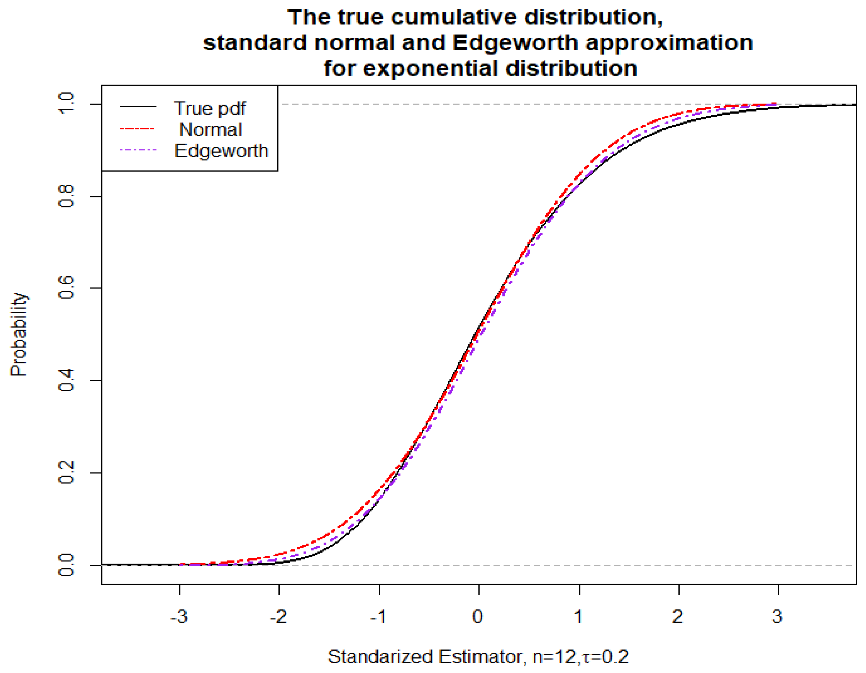
Figure 2.
True cdf, normal, and Edgeworth approximation for the studentized estimator with exponential data.
Figure 2.
True cdf, normal, and Edgeworth approximation for the studentized estimator with exponential data.
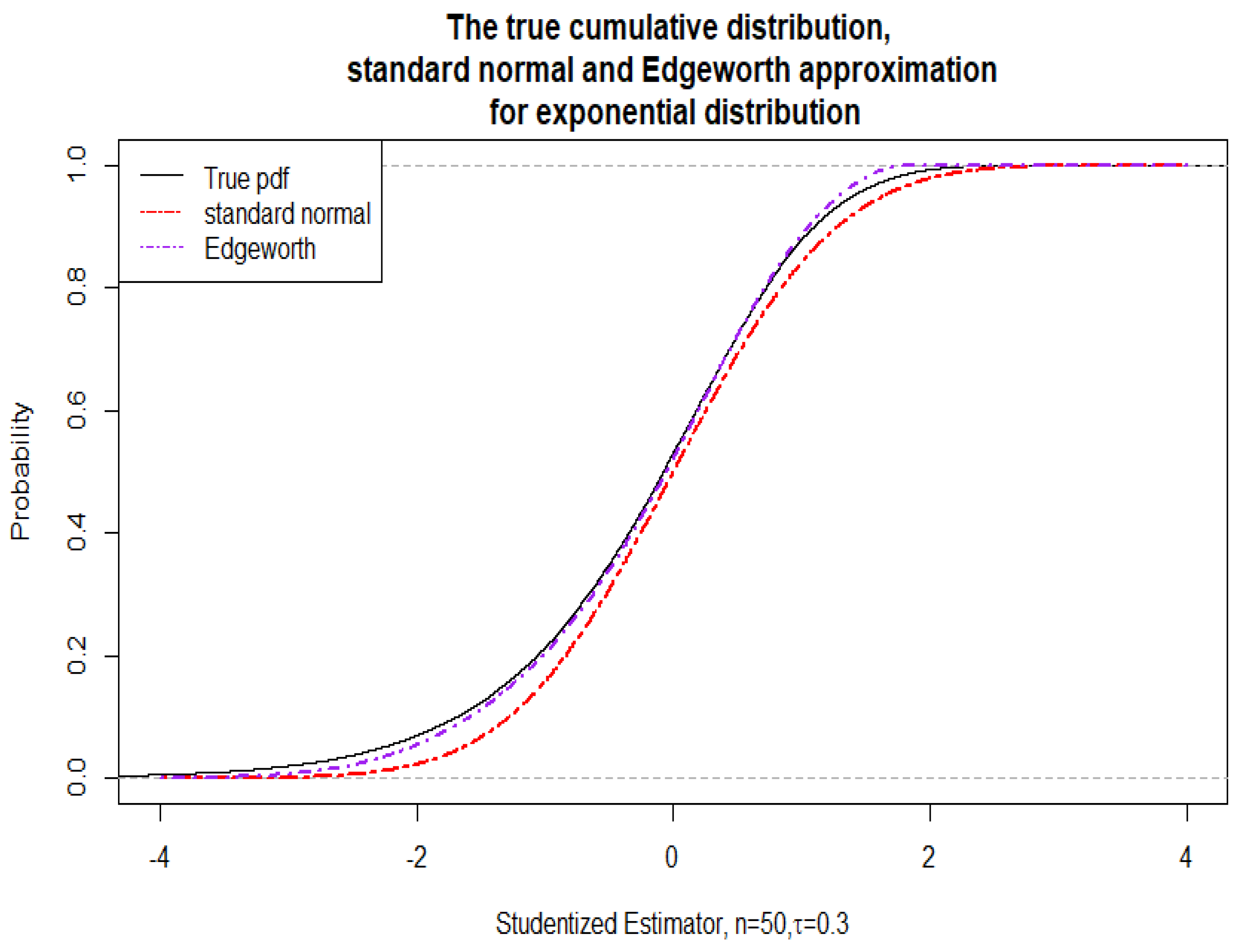

Table 1.
Symmetric confidence intervals for the expectile of the standard exponential distribution
| Sample size | Nominal coverage | |||
| Normal | Numerical inversion | CF method | ||
| 20 | 0.5 | 0.85630 | 0.85730 | |
| 20 | 0.4 | 0.84648 | 0.83894 | |
| 20 | 0.3 | 0.83056 | 0.81052 | |
| 20 | 0.2 | 0.80674 | 0.76108 | |
| 20 | 0.1 | 0.75308 | 0.66668 | |
| 50 | 0.5 | 0.88008 | 0.87974 | |
| 50 | 0.4 | 0.87504 | 0.86940 | |
| 50 | 0.3 | 0.86872 | 0.85496 | |
| 50 | 0.2 | 0.85734 | 0.82832 | |
| 50 | 0.1 | 0.82998 | 0.76416 | |
| 100 | 0.5 | 0.89244 | 0.89138 | |
| 100 | 0.4 | 0.88938 | 0.88616 | |
| 100 | 0.3 | 0.88588 | 0.87762 | |
| 100 | 0.2 | 0.87834 | 0.86204 | |
| 100 | 0.1 | 0.86184 | 0.82268 | |
| 150 | 0.5 | 0.89558 | 0.89476 | |
| 150 | 0.4 | 0.89284 | 0.89164 | |
| 150 | 0.3 | 0.89070 | 0.88544 | |
| 150 | 0.2 | 0.88532 | 0.87424 | |
| 150 | 0.1 | 0.87374 | 0.84714 | |
| 200 | 0.5 | 0.89714 | 0.89666 | |
| 200 | 0.4 | 0.89522 | 0.89374 | |
| 200 | 0.3 | 0.89330 | 0.88916 | |
| 200 | 0.2 | 0.88714 | 0.88008 | |
| 200 | 0.1 | 0.88094 | 0.86120 | |
Table 2.
Symmetric confidence intervals for the expectile of the standard exponential distribution
| Sample size | Nominal coverage | |||
| Normal | Numerical inversion | CF method | ||
| 20 | 0.5 | 0.90454 | 0.91170 | |
| 20 | 0.4 | 0.89414 | 0.89408 | |
| 20 | 0.3 | 0.87992 | 0.86164 | |
| 20 | 0.2 | 0.85692 | 0.80174 | |
| 20 | 0.1 | 0.80530 | 0.69500 | |
| 50 | 0.5 | 0.93000 | 0.93170 | |
| 50 | 0.4 | 0.92404 | 0.92260 | |
| 50 | 0.3 | 0.91726 | 0.90848 | |
| 50 | 0.2 | 0.90608 | 0.87640 | |
| 50 | 0.1 | 0.87604 | 0.79596 | |
| 100 | 0.5 | 0.94104 | 0.94194 | |
| 100 | 0.4 | 0.93896 | 0.93718 | |
| 100 | 0.3 | 0.93500 | 0.92922 | |
| 100 | 0.2 | 0.92642 | 0.91332 | |
| 100 | 0.1 | 0.90554 | 0.86584 | |
| 150 | 0.5 | 0.94426 | 0.94580 | |
| 150 | 0.4 | 0.94230 | 0.94266 | |
| 150 | 0.3 | 0.93858 | 0.93744 | |
| 150 | 0.2 | 0.93386 | 0.92570 | |
| 150 | 0.1 | 0.91924 | 0.89484 | |
| 200 | 0.5 | 0.94588 | 0.94688 | |
| 200 | 0.4 | 0.94478 | 0.94372 | |
| 200 | 0.3 | 0.94282 | 0.93926 | |
| 200 | 0.2 | 0.93688 | 0.93140 | |
| 200 | 0.1 | 0.92606 | 0.90954 | |
Disclaimer/Publisher’s Note: The statements, opinions and data contained in all publications are solely those of the individual author(s) and contributor(s) and not of MDPI and/or the editor(s). MDPI and/or the editor(s) disclaim responsibility for any injury to people or property resulting from any ideas, methods, instructions or products referred to in the content. |
© 2024 by the authors. Licensee MDPI, Basel, Switzerland. This article is an open access article distributed under the terms and conditions of the Creative Commons Attribution (CC BY) license (http://creativecommons.org/licenses/by/4.0/).
Copyright: This open access article is published under a Creative Commons CC BY 4.0 license, which permit the free download, distribution, and reuse, provided that the author and preprint are cited in any reuse.


