
Submitted:
17 December 2024
Posted:
18 December 2024
You are already at the latest version
Abstract
Hail disaster prediction is a pivotal research topic within the field of meteorology, carrying substantial importance for the prevention and mitigation of disasters. The complex terrain and frequent occurrence of hail in Qinghai Province present challenges for traditional prediction methods, which are hindered by issues such as sample imbalance and geographic complexity, resulting in less than ideal outcomes. This study, based on ERA5 reanalysis data and ground-based observation records, proposes a LightGBM hail prediction model that integrates Bayesian optimization with a dual-output header (DOH) structure. First, the DOH structure is developed to separately optimize positive and negative samples, effectively mitigating the sample imbalance problem. Additionally, a Bayesian optimization strategy is applied to conduct global hyperparameter tuning, thereby improving model performance. Experimental results show that, compared to mainstream single and ensemble classification methods, the proposed model achieves superior accuracy, precision, and recall. In the test set, the model demonstrated a prediction accuracy of 0.97, a recall of 0.939, a precision of 0.966, a critical success index (CSI) of 0.909, and a false alarm rate (FAR) of only 0.015. This research provides an effective technical solution for hail prediction in the Qinghai region, offering significant practical value for enhancing early warning capabilities.
Keywords:
hail prediction models
; LightGBM
; Qinghai Province
; Bayesian optimization
; imbalanced samples
1. Introduction
Hail is a violent weather phenomenon caused by a strong convective system. Although hail occurs in a small area and lasts for a short period of time, it is sudden and destructive, including damage to vehicles and houses, complete destruction of crops and so on, which significantly impacts socio-economic development , daily life and food security [1]. According to statistics, hail disasters have caused huge economic losses worldwide [2,3], and particularly in China, the annual direct economic losses caused by hail exceed 2 billion yuan [4]. According to meteorological statistics, China is one of the areas in the world with a high incidence of hail disasters. Due to its special topographical conditions and large-scale circulation background, the Qinghai-Tibet Plateau has a significantly higher annual average number of hail days than other regions of China [5]. The Qinghai-Tibet Plateau is the highest and widest plateau in the world, and it is also one of the regions which are very sensitive to climate change [6,7]. Qinghai Province is located in the hinterland of the Qinghai-Tibet Plateau, with a complex terrain and a changeable climate. It is a high-risk area for hail [8,9,10].
One of the main obstacles to study hail events and their climatology is the lack of accurate and comprehensive observations [11]. Hail research in China began in the 1960s, but there were no systematic research results on nationwide hail events until 2008. Research is still relatively limited, and hail forecasting is difficult due to differences in hail observation data standards and complex climatic conditions [12]. Hail forecasting methods have gradually evolved from traditional empirical forecasting based on natural phenomena to modern forecasting systems that use techniques such as numerical weather models, radar, machine learning, and neural networks. These include ensemble forecasting, dual-polarization radar, and the WRF-HAILCAST model, which have significantly improved the accuracy and reliability of hail forecasting [13]. Current hail forecasting mainly relies on a variety of machine learning methods, such as random forests, gradient boosted trees, and linear regression, to identify and predict hail by combining multidimensional data such as radar data, sounding data, automatic station statistics, and terrain. These models can not only analyze the structure of storms in the atmosphere, but also predict the size and probability of hail based on input weather parameters and local characteristics, further improving the spatial and temporal resolution of forecasts [14,15,16,17].
In recent years, machine learning algorithms have shown significant potential in the field of hail forecasting. Many researchers have used a variety of machine learning methods to conduct in-depth empirical studies in different regions and have made a series of breakthroughs. Yuan et al. analyzed the characteristics of hail disasters in the eastern part of Wuhan based on decision tree algorithms, and innovatively combined Doppler radar observation data, sounding data, and key physical quantities such as wet bulb temperature and height to construct a hail event recognition model [18]. In the Shandong Peninsula region, Yao et al. proposed an improved random forest-based approach. By using measured data from weather stations, combined with convective indices and key physical quantities from reanalysis data, they developed a hail warning model for a 0-6 hour forecast window [19]. Xin et al. constructed a comprehensive classification identification model based on the LightGBM algorithm that can simultaneously identify various hazardous weather phenomena such as hail, thunderstorm gusts, and short-term heavy precipitation by integrating C-band radar echo products and ground observation data [20]. Decision tree algorithms, random forest algorithms, and LightGBM algorithms are all ensemble learning algorithms. On unbalanced datasets, the LightGBM algorithm generally exhibits better performance [21,22].
Reanalysis data is a widely used source of climate data for studying severe weather environments [23]. The ERA5 reanalysis dataset is the fifth generation of atmospheric reanalysis data developed by the European Centre for Medium-Range Weather Forecasts (ECMWF). It reconstructs the global atmospheric, land, and ocean conditions from 1940 to the present day [24]. The ERA5 reanalysis dataset can accurately characterize the large-scale circulation characteristics and mesoscale convective environment during hail weather. Its high-spatial-resolution atmospheric element fields provide reliable data support for accurately characterizing convective instability and dynamic conditions [25].
Qinghai Province is a high-risk area for hail in China. Its unique geographical location and complex climatic conditions make hail forecasting significantly more difficult, and hail has caused huge economic losses in local agriculture, construction, transportation and other fields [26]. However, there have been relatively few studies on hail forecasting in Qinghai Province. The existing literature lacks discussion on the formation mechanism of hail, forecasting models and their applications. Against this research background, this paper aims to construct an innovative hail prediction framework for the complex terrain area of Qinghai Province. Considering the topographic characteristics of the research area and the challenge of severe imbalance in hail samples, this study proposes two key improvements based on the efficient LightGBM model combined with ERA5 data: First, breaking through the limitations of the traditional binary classification loss function [27], an innovative designed the DOH (Dual Output Header) optimization algorithm, which effectively alleviates the constraints on model performance caused by the unbalanced hail samples. Second, a Bayesian optimization strategy is introduced to significantly enhance the global optimization capability of the model through systematic parameter space exploration [28].
The main contributions of this study are as follows:
- A Bayesian-DOH-LightGBM hail prediction framework is constructed and verified using the Qinghai Province hail dataset, and the results show that the framework can improve the performance of hail prediction;
- The proposed DOH algorithm achieves a separate optimization strategy for different categories by innovatively using dual-output head optimization;
- The introduction of a Bayesian optimization strategy not only effectively improves the accuracy, but also significantly reduces the time consumption of hyperparameter tuning.
The rest of this paper is organized as follows. The Section 2 details the data selection and preprocessing procedures, explains the principles of the LightGBM algorithm, the DOH optimization method, the Bayesian optimization strategy, and the evaluation metrics used, and describes the proposed hail prediction framework. The Section 3 demonstrates the model construction process, verifies the performance of the DOH optimization and Bayesian optimization methods, and evaluates the effectiveness of the hail prediction framework through comparative experiments. The Section 4 conducts sensitivity analysis of input features and analysis of the probability density estimation curves of feature factors, summarizes the main findings and contributions of this research. Finally, the Section 5 discusses the limitations of hail prediction research, and proposes future research directions.
2. Data and Methods
2.1. Bayesian-DOH-LightGBM Prediction Model Framework
Based on the research background and theoretical foundation presented earlier, this chapter proposes an improved LightGBM model that integrates Bayesian optimization with a dual-output head (DOH) structure to enhance hail prediction accuracy. To clearly illustrate the overall architecture and workflow of the model, a comprehensive prediction framework is constructed. The Bayesian-DOH-LightGBM hail prediction flowchart, shown in Figure 1, consists of four modules.
The ERA5 and Hail Label Data Preprocessing Module (A) prepares high-quality data by aligning ERA5 reanalysis features with hail event labels. The DOH Optimization Module (B) improves model performance by introducing two output heads, each optimized for different categories using tailored binary classification loss functions. The Bayesian Optimization Module (C) accelerates the search for optimal model parameters, enhancing both efficiency and accuracy. Finally, the Model Construction and Evaluation Module (D) evaluates model performance using key metrics, including Precision, FAR, CSI, Accuracy, and Recall, ensuring effective hail prediction.
These modules work together to streamline data processing, model optimization, and performance evaluation.
2.2. Data
The hail event data in this study were obtained from records of 52 ground-based meteorological observation stations and the disaster reporting system in Qinghai Province, covering the period from 2009 to 2023. Meteorological features were derived from the ERA5 global atmospheric reanalysis dataset by ECMWF, which has a spatial resolution of 0.25° × 0.25° and an hourly temporal resolution. This study focuses on temperature (t), geopotential height (z), divergence (d), vertical velocity (w), and wind components (u, v) across eight pressure levels (20–600 hPa). Additionally, surface layer features such as CAPE, integrated temperature (p54.162), thermal energy (p60.162), moisture flux (p84.162), water vapor flux (vimd), instantaneous water flux (ie), 2-meter dew point temperature (d2m), and the zero-degree level (deg0l) were included.
2.3. Data Preprocessing
This study integrates multi-source heterogeneous data, combining ground-based meteorological observations, hail disaster records, and ERA5 reanalysis data to enhance data coverage and feature diversity [29]. The fusion approach leverages the complementary spatial and temporal characteristics of these sources, enriching feature sets and improving model precision by uncovering latent patterns and correlations.
To address temporal inconsistencies, we unified the temporal resolution of the ground observations and disaster records with the hourly resolution of the ERA5 dataset. This was achieved through a time label expansion strategy, assigning a value of 1 (hail occurrence) to all 24 hourly intervals of a recorded hail event. Spatial discrepancies were resolved using nearest neighbor interpolation, mapping observation sites and disaster reports to the closest ERA5 grid points (0.25° × 0.25°). The resulting dataset spans Qinghai Province, covering 31°–40°N and 89°–104°E [30].
Figure 2 illustrates the data preprocessing workflow. We performed spatiotemporal fusion of ERA5 data across multiple pressure levels and surface layers, mapping the fused data to the Qinghai Province region and aligning it with hail observation and disaster record data. This process resulted in a unified initial dataset with a spatial resolution of 0.25° × 0.25° and a temporal resolution of 1 hour, effectively integrating the strengths of ground observations, disaster reports, and atmospheric reanalysis data.
However, due to the rarity of hail events, the initial dataset exhibited a significant class imbalance, with negative samples (non-hail events) overwhelmingly outnumbering positive samples (hail events). This imbalance can lead to models favoring the majority class while overlooking the minority class [31]. To address this issue, we employed an undersampling strategy for the majority class, as it is less prone to introducing data bias compared to oversampling the minority class [32]. By retaining all positive samples (hail events) and randomly selecting a subset of negative samples, we adjusted the positive-to-negative sample ratio to 1:1.35. This approach resulted in a balanced experimental dataset, which was then split into training (2009–2021), validation (2022), and independent testing (2023) sets based on the year. The sample sizes of the three data sets are shown in Table 1.
2.4. DOH Optimization Method
Before constructing the hail prediction model in this study, it is essential to introduce the foundational algorithm framework. The LightGBM model used in this study is an improved version of the Gradient Boosting Decision Tree (GBDT). GBDT is an ensemble learning algorithm that builds a predictive model by iteratively combining multiple decision trees [33,34].
Figure 3 illustrates the workflow of GBDT. Starting with an initial model , the algorithm iterates through multiple steps. In each iteration, the residuals between the predicted and actual hail values are calculated, and a new decision tree is fitted based on these residuals, updating the model accordingly. This process involves iteratively adjusting model parameters. By progressively enhancing the performance of individual weak learners, GBDT combines them into a robust ensemble model, which accurately predicts the spatiotemporal patterns of hail occurrences based on historical meteorological data and hail disaster records, thus improving both prediction accuracy and timeliness [35,36].
In this study, the baseline model employs LightGBM, a gradient boosting decision tree (GBDT) algorithm optimized for large-scale sparse data [37]. Unlike traditional GBDT methods, LightGBM incorporates two key techniques: Gradient-based One-Side Sampling (GOSS) and Exclusive Feature Bundling (EFB) [38]. As shown in Figure 4, GOSS optimizes sample-level importance by retaining samples with large gradients, ensuring that the most critical samples for model improvement are preserved during training. EFB, on the other hand, reduces the feature dimension by bundling mutually exclusive features together, effectively retaining key information. These optimizations enable LightGBM to significantly enhance computational efficiency while maintaining high prediction accuracy when dealing with large-scale sparse data [39].
This method draws on the optimization strategies of GBDT and LightGBM, leveraging their strengths in handling large-scale sparse data and improving model efficiency. To further enhance model performance in hail prediction, particularly in addressing the issue of class imbalance, this study proposes an innovative Dual-Output Head (DOH) structure. While LightGBM performs excellently on large-scale sparse data due to its efficient algorithmic optimization techniques, class imbalance remains a major challenge in hail prediction tasks. To address this, the DOH structure designs independent loss functions for each class, selecting distinct binary classification loss functions for hail events (the minority class) and non-hail events (the majority class). This approach increases the model’s sensitivity to the minority class (hail events) while maintaining performance on the majority class (non-hail events), effectively improving the overall accuracy and predictive capability of the model on imbalanced datasets.
To address the class imbalance issue, the DOH structure utilizes two distinct loss functions, each tailored to the specific needs of the minority and majority classes. For hail events (the minority class), we adopt the Focal Loss, which is specifically designed to down-weight the impact of well-classified examples and focus more on hard-to-classify instances. This approach helps to mitigate the imbalance by ensuring the model places more emphasis on rare hail events. For non-hail events (the majority class), we employ Binary Cross-Entropy Loss, a commonly used loss function in binary classification tasks, which helps maintain robust performance on the majority class. By using these separate loss functions, the model can simultaneously optimize for sensitivity to the minority class and performance on the majority class, thus improving overall predictive accuracy on imbalanced datasets. The details of these two loss functions are described as follows:
Binary Cross-Entropy (BCE) loss is a widely used loss function for binary classification tasks. It quantifies the difference between the model’s predicted probability () and the true label (y, either 0 or 1) [40]. The BCE loss, as expressed in Equation (4), is defined as follows in Equation (1):
Focal Loss is designed to address class imbalance in tasks like object detection by focusing on hard-to-classify samples. Standard cross-entropy (CE) loss treats all samples equally, which can cause the model to be dominated by easily classified negative samples [41]. To mitigate this, a weighting factor is introduced to balance the contribution of each class, as shown in Equation (2):
Here is the predicted probability, and adjusts for class imbalance [42].
Focal Loss extends CE loss by adding a modulation factor , which reduces the loss weight of easy samples and emphasizes hard-to-classify ones. When , Focal Loss simplifies to balanced CE loss. As increases, the focus shifts to difficult samples, as shown in Equation (3):
2.5. Bayesian Optimization Method
Bayesian optimization is an efficient global optimization algorithm designed to find the optimal solution with minimal cost. It addresses the challenge of selecting the next evaluation point based on information gathered from the unknown objective function, thereby accelerating the process toward the optimal solution. By using a probabilistic surrogate model and an acquisition function, Bayesian optimization avoids unnecessary sampling, making it more efficient than traditional methods such as grid search or random search [43].
The process involves iteratively training a surrogate model with initial data, selecting the next evaluation point using the acquisition function, and updating the model based on the new data. This cycle continues until a convergence criterion is met. By balancing exploration of unknown regions with the exploitation of known beneficial regions, Bayesian optimization efficiently converges to a global or local optimum.
2.6. Evaluation Metrics
This study evaluates the performance of the decision tree algorithm in hail identification using several metrics: precision, false alarm ratio (FAR), critical success index (CSI), accuracy, F1-score, and recall [44]. The formulas for these metrics are shown in Equations (4)–(9). In this context, hail samples are labeled as positive (1) and non-hail samples as negative (0). True Positive (TP) refers to correctly predicted positive cases, True Negative (TN) to correctly predicted negative cases, False Positive (FP) to negative cases incorrectly predicted as positive, and False Negative (FN) to positive cases incorrectly predicted as negative. These metrics provide a comprehensive assessment of the model’s performance, particularly in the case of imbalanced datasets.
3. Experimental Results
3.1. Model Construction
In the feature engineering stage, hail occurrence (whether hail occurs or not) is designated as the target variable (label), while various meteorological and environmental parameters are used as predictors. These predictors form the input feature space for the model, enabling it to learn the patterns and relationships essential for hail prediction.
To improve model performance, we leverage the Bayesian-DOH-LightGBM framework, which features a dual-output head (DOH) architecture. Each output head independently predicts a specific target: and , where and are the parameters for each head. Here, and are the predicted outputs corresponding to each output head. The total loss function is as shown in Equation 10.
Where and are the individual loss functions for the two heads, and and control the contribution of each head to the total loss. The ground truth label, y, is shared between the two heads. Bayesian optimization is employed to tune not only the model parameters and , but also the weights and , ensuring an optimal balance between the two tasks. This framework allows each output head to specialize in its respective task while improving the overall performance of the model. Finally, the model is validated on an independent dataset to confirm its generalization ability.
3.2. Optimization Method Performance Verification
3.2.1. Performance test of DOH optimization method
To determine the optimal classification threshold for the hail identification model, this study uses the Receiver Operating Characteristic (ROC) curve for analysis. The ROC curve illustrates the relationship between the True Positive Rate (TPR) and False Positive Rate (FPR) across different decision thresholds, providing a comprehensive evaluation of classifier performance [45]. As shown in Figure 5, when applying Focal Loss as the loss function for the LightGBM model, we analyzed the ROC curve performance for various combinations of the Alpha (weighting factor, ) and Gamma (modulation factor, ) parameters [46]. By balancing the model’s sensitivity and specificity, we found that setting the classification threshold to 0.4 resulted in the best predictive performance.
To determine the optimal Alpha () and Gamma () parameters, we first set the range of values between 0 and 1, initializing =0.4. Subsequently, we analyzed the model’s accuracy, precision, and F1-score [47] across various Gamma values while keeping =0.4 (left graph in Figure 6). The results indicate that the model achieves its best overall performance when =2.75.
Next, with fixed at 2.75, we further examined the accuracy, precision, and F1-score for different values (right graph in Figure 6). Based on these analyses, we concluded that the model exhibits superior performance when =0.5 and =2.75.
To evaluate the effectiveness of the proposed DOH architecture, we conducted an ablation study comparing single-output and dual-output configurations. The single-output models included Single-BCE, which optimized the BCE loss, and Single-Focal, which utilized the Focal loss. The dual-output models included the FB configuration, where the first output head was optimized with the Focal loss for hail prediction and the second with BCE loss for non-hail prediction, and the BF configuration, which reversed this sequence. Results, summarized in Table 2, show that Single-BCE performed well in terms of precision but struggled with minority class recognition due to class imbalance, while Single-Focal improved minority class recognition at the expense of overall accuracy. The dual-output models demonstrated superior performance, with the FB configuration achieving the best balance across metrics such as precision, accuracy and f1-score. This suggests that prioritizing the Focal loss in the first head better addresses class imbalance and enhances overall performance, highlighting the effectiveness of the DOH architecture in hail prediction tasks.
3.2.2. Performance Validation of Bayesian Optimization
To quantitatively evaluate the computational efficiency and model performance of the Bayesian hyperparameter optimization algorithm, we conducted a comparative experiment involving three commonly used parameter search methods: grid search, random search, and Bayesian optimization [48,49]. The experiment utilized two datasets: the Wine Dataset from the UCI Machine Learning Repository [50] as a benchmark and a random subset of the Hail Dataset, constructed for domain-specific evaluation. Two metrics were used: time consumption to assess computational efficiency and accuracy to evaluate prediction performance. Each algorithm was run multiple times on both datasets to ensure statistical significance. The results, summarized in Table 3, show that Bayesian optimization consistently outperforms grid and random search in terms of time efficiency, while achieving comparable prediction accuracy. These findings demonstrate the effectiveness of Bayesian optimization in reducing computational costs while maintaining robust performance across diverse datasets.
3.3. Comparative Experiment
3.3.1. Parameter optimization based on Bayesian optimization algorithm
Since the general process of Bayesian optimization has been introduced earlier, this section focuses on its application to the DOH-LightGBM model. Specifically, the algorithm optimizes key hyperparameters such as num-leaves, learning-rate, and feature-fraction by iteratively refining the posterior distribution using Gaussian process regression. The objective function is set to maximize model accuracy on the validation set. The optimization process continuously updates the hyperparameter space through an acquisition function, ensuring the selection of the most promising parameter combinations. Table 4 summarizes the optimal hyperparameters and corresponding model performance achieved through this process.
3.3.2. Comparison of the Bayesian-DOH-LightGBM model with other classification models
To further evaluate the predictive performance of the Bayesian-DOH-LightGBM model, we compared it against several widely used classification models. These include traditional single classifiers such as Decision Tree and KNN, as well as popular ensemble learning models like Random Forest, XGBoost, AdaBoost, LightGBM, and Bayesian-LightGBM [51,52,53]. The comparative results are presented in Table 5. The experimental results indicate that the Bayesian-DOH-LightGBM model proposed in this study surpasses other models in key metrics such as precision, FAR, CSI, and accuracy. While its recall is slightly lower than that of the LightGBM model (ranked second), the overall predictive performance remains significantly superior to both mainstream ensemble learning classifiers and single classifiers, highlighting its exceptional comprehensive capabilities.
Figure 7 presents a comparison of the confusion matrices for the baseline LightGBM model and the enhanced Bayesian-DOH-LightGBM model on the test set. The results reveal that the Bayesian-DOH-LightGBM model achieves notable improvements in key performance metrics: the false alarm rate (FAR) is reduced by 2.8% (from 4.3% to 1.5%), and the precision increases by 5.8% (from 90.8% to 96.6%). These findings demonstrate that the Bayesian-DOH-LightGBM model delivers more balanced and robust classification performance in the hail prediction task.
4. Discussion
4.1. Input Feature Sensitivity Analysis
To analyze the sensitivity of features and their impact on hail prediction, this study employs SHAP (SHapley Additive exPlanations), a model interpretation method based on Shapley values from game theory. SHAP calculates the marginal contribution of each feature to the prediction outcome, quantifying its importance in the hail classification model [54]. A higher SHAP value indicates a greater influence of the feature on the model’s decision-making process.
Figure 8 displays the distribution of the top ten features ranked by SHAP values in the Bayesian-DOH-LightGBM model. Key features such as p54.162, p60.162, and d2m exhibit the highest SHAP values, highlighting their critical roles in influencing tropospheric stability, convection intensity, moisture transport, and local weather systems—factors that significantly determine hail occurrence and severity.The geopotential height (z) and zonal wind (u) at different pressure levels (indicated by the numbers following the variables, such as z20 at 20hPa and u500 at 500hPa) are also identified as significant predictors. These meteorological parameters collectively determine hail occurrence and severity through their interactions in the atmosphere.
4.2. Analysis of Feature Factor Kernel Density Estimation Curves
Kernel density estimation (KDE) curves are used to estimate the probability density of feature values across data samples, providing a smooth representation of the feature distribution. Unlike histograms, KDE curves better illustrate the overall trends and underlying patterns in the data. In classification tasks, the KDE curve helps analyze the relationship between features and the target variable, revealing distribution differences across classes and offering valuable insights for model optimization and feature selection [55].
Figure 9 shows the KDE curves for the top six SHAP-ranked features (p54.162, p60.162, d2m, t100, u500, z20). Solid lines represent feature distributions in hail samples, while dashed lines represent those in non-hail samples. The curves for p54.162, p60.162, and d2m show distinct peaks in hail samples, indicating strong discriminatory power for hail events. These features are thus valuable indicators for hail prediction. In contrast, most other features lack significant separability, suggesting they have less impact on classification. Therefore, considering multiple key features and their interactions is crucial for improving prediction accuracy.
4.3. Discussion and Analysis
This study enhances the performance of the LightGBM model for hail prediction in Qinghai Province by integrating the Bayesian optimization algorithm with a dual-output head (DOH) structure, addressing challenges such as data imbalance and the need for high-precision predictions. The proposed Bayesian-DOH-LightGBM framework tackles key issues like data scarcity, class imbalance, and the complexity of multi-scale weather systems typical in hail prediction.
The DOH optimization, particularly the BF output head, outperforms other heads in terms of accuracy, hit rate, and F1-score. By applying different binary classification loss functions for hail and non-hail categories, the BF output head improves the model’s sensitivity to the minority class (hail), thus enhancing prediction accuracy.
Performance evaluation of the Bayesian optimization algorithm shows a significant advantage in computational efficiency. Compared to traditional methods, Bayesian optimization reduces computation time by nearly 10-fold relative to grid search and is 20% faster than random search, while maintaining comparable or superior prediction accuracy.
The Bayesian-DOH-LightGBM model outperforms both individual and ensemble classifiers. It achieves the highest hit rate, false alarm rate, critical success index, and overall accuracy on an independent test set. The reduction in misclassifications of hail events underscores the model’s effectiveness in improving prediction performance.
5. Conclusions and Future Work
This study demonstrates the effectiveness of integrating the Bayesian optimization algorithm with a dual-output head (DOH) structure to enhance the LightGBM model’s performance in hail prediction for Qinghai Province. The proposed Bayesian-DOH-LightGBM framework successfully addresses key challenges, including data scarcity, class imbalance, and the complexity of multi-scale weather systems. By improving the model’s sensitivity to hail events and applying Bayesian optimization to accelerate training while maintaining high accuracy, this approach outperforms traditional search methods and demonstrates superior prediction performance.
However, several challenges remain. The scarcity of hail data, compounded by severe class imbalance, makes it difficult for models to accurately capture hail formation patterns. As a rare phenomenon, hail events are vastly outnumbered by non-hail events, leading to a high false negative rate, especially when hail is imminent. Additionally, the complex multi-scale nature of convective weather systems and the limited resolution of existing meteorological data hinder precise predictions. The uneven distribution of meteorological stations in Qinghai Province further complicates timely data collection.
Future research will focus on incorporating high-resolution radar, satellite remote sensing, and numerical weather prediction model outputs to improve the capture of local weather details. Additionally, efforts will be made to develop more robust machine learning models capable of overcoming data scarcity and class imbalance while capturing the multi-scale dynamics of weather systems for enhanced hail prediction.
Funding
This research was funded by the Natural Science Foundation of Qinghai Province (No. 2023-ZJ-906M) and the National Natural Science Foundation of China (No. 62162053, No.42265010 ).
Informed Consent Statement
Not applicable.
Data Availability Statement
The datasets generated and analyzed during the current study are available from the corresponding author upon reasonable request. The hail data, which cannot be made publicly available, were obtained from the Qinghai Meteorological Bureau, and the feature factor data were sourced from the publicly available ERA5 dataset provided by the European Centre for Medium-Range Weather Forecasts (ECMWF).
Acknowledgments
This paper is supported by the high-performance computing center at Qinghai University.
Conflicts of Interest
The authors declare no conflict of interest.
References
- Xingzhi, T.; Rong, Z.; Wenyu, W.; others. Temporal and spatial distribution characteristics of hail disaster events in China from 2010 to 2020. Torrential Rain and Disasters 2023, 42, 223–231.
- Fluck, E.; Kunz, M.; Geissbuehler, P.; Ritz, S.P. Radar-based assessment of hail frequency in Europe. Natural Hazards and Earth System Sciences 2021, 21, 683–701. [Google Scholar] [CrossRef]
- Brook, J.P.; Protat, A.; Soderholm, J.; Carlin, J.T.; McGowan, H.; Warren, R.A. HailTrack—Improving radar-based hailfall estimates by modeling hail trajectories. Journal of Applied Meteorology and Climatology 2021, 60, 237–254. [Google Scholar] [CrossRef]
- Qing-zu, L.; Peng-jie, D.; Cai-hua, Y. A Weather-index-based Insurance-oriented Method for Hail Disaster Assessment on Fruits Loss. Chinese Journal of Agrometeorology 2019, 40, 402. [Google Scholar]
- MA Xiaoling, LI Deshuai, H.S. Analysis of Spatio-Temporal Characteristics of Thunderstorm and Hail over Qinghai Province. Meteorological Monthly 2020, 46, 301–312.
- Li, M.; Zhang, Q.; Zhang, F. Hail day frequency trends and associated atmospheric circulation patterns over China during 1960–2012. Journal of Climate 2016, 29, 7027–7044. [Google Scholar] [CrossRef]
- Sun, S.; Zhang, Q.; Xu, Y.; Yuan, R. Integrated assessments of meteorological hazards across the Qinghai-Tibet Plateau of China. Sustainability 2021, 13, 10402. [Google Scholar] [CrossRef]
- al, W.S.Y.C. Comprehensive risk management of multiple natural disasters on the Qinghai-Tibet Plateau. Journal of Glaciology and Geocryology 2021, 43, 1848–1860. [Google Scholar]
- Ji, B.; Xiong, Q.; Xing, P.; Qiu, P. Dynamic response characteristics of heliostat under hail impacting in Tibetan Plateau of China. Renewable Energy 2022, 190, 261–273. [Google Scholar] [CrossRef]
- Shuai, H.; Yan-ling, S.; Shuang, S.; Chun-yi, W. Review on the impacts of climate change on highland barley production in Tibet Plateau. Chinese Journal of Agrometeorology 2023, 44, 398. [Google Scholar]
- Fluck, E.; Kunz, M.; Geissbuehler, P.; Ritz, S.P. Radar-based assessment of hail frequency in Europe. Natural Hazards and Earth System Sciences 2021, 21, 683–701. [Google Scholar] [CrossRef]
- Allen, J.T.; Giammanco, I.M.; Kumjian, M.R.; Jurgen Punge, H.; Zhang, Q.; Groenemeijer, P.; Kunz, M.; Ortega, K. Understanding hail in the earth system. Reviews of Geophysics 2020, 58, e2019RG000665. [Google Scholar] [CrossRef]
- Kim, M.H.; Lee, J.; Lee, S.J. Hail: Mechanisms, Monitoring, Forecasting, Damages, Financial Compensation Systems, and Prevention. Atmosphere 2023, 14, 1642. [Google Scholar] [CrossRef]
- Gagne, D.; McGovern, A.; Jerald, J.; Coniglio, M.; Correia, J.; Xue, M. Day-ahead hail prediction integrating machine learning with storm-scale numerical weather models. Proceedings of the AAAI Conference on Artificial Intelligence, 2015, Vol. 29, pp. 3954–3960.
- Czernecki, B.; Taszarek, M.; Marosz, M.; Półrolniczak, M.; Kolendowicz, L.; Wyszogrodzki, A.; Szturc, J. Application of machine learning to large hail prediction-The importance of radar reflectivity, lightning occurrence and convective parameters derived from ERA5. Atmospheric Research 2019, 227, 249–262. [Google Scholar] [CrossRef]
- Burke, A.; Snook, N.; Gagne II, D.J.; McCorkle, S.; McGovern, A. Calibration of machine learning–based probabilistic hail predictions for operational forecasting. Weather and Forecasting 2020, 35, 149–168. [Google Scholar] [CrossRef]
- Zhang, Y.; Ji, Z.; Xue, B.; Wang, P. A novel fusion forecast model for hail weather in plateau areas based on machine learning. Journal of Meteorological Research 2021, 35, 896–910. [Google Scholar] [CrossRef]
- Yuan Kai, L.W.; Jing, P. Hail identification technology in Eastern Hubei based on decision tree algorithm. J Appl Meteor Sci 2023, 34, 234–245. [Google Scholar]
- Yao, H.; Li, X.; Pang, H.; Sheng, L.; Wang, W. Application of random forest algorithm in hail forecasting over Shandong Peninsula. Atmospheric research 2020, 244, 105093. [Google Scholar] [CrossRef]
- Xinwei LIU and Wubin HUANG and Yingsha JIANG and Runxia GUO and Yuxia HUANG and Qiang SONG and Yong YANG. Study of the Classified Identification of the Strong Convective Weathers Based on the LightGBM Algorithm. Plateau Meteorology 2021, 40, 909–918.
- Sari, L.; Romadloni, A.; Lityaningrum, R.; Hastuti, H.D. Implementation of LightGBM and Random Forest in Potential Customer Classification. TIERS Information Technology Journal 2023, 4, 43–55. [Google Scholar] [CrossRef]
- Choudhury, A.; Mondal, A.; Sarkar, S. Searches for the BSM scenarios at the LHC using decision tree-based machine learning algorithms: a comparative study and review of random forest, AdaBoost, XGBoost and LightGBM frameworks. The European Physical Journal Special Topics, 2024; 1–39. [Google Scholar]
- Taszarek, M.; Pilguj, N.; Allen, J.T.; Gensini, V.; Brooks, H.E.; Szuster, P. Comparison of convective parameters derived from ERA5 and MERRA-2 with rawinsonde data over Europe and North America. Journal of Climate 2021, 34, 3211–3237. [Google Scholar] [CrossRef]
- Hersbach, H.; Bell, B.; Berrisford, P.; Hirahara, S.; Horányi, A.; Muñoz-Sabater, J.; Nicolas, J.; Peubey, C.; Radu, R.; Schepers, D.; et al. The ERA5 global reanalysis. Quarterly Journal of the Royal Meteorological Society 2020, 146, 1999–2049. [Google Scholar] [CrossRef]
- Pilorz, W.; Laskowski, I.; Surowiecki, A.; Taszarek, M.; Łupikasza, E. Comparing ERA5 convective environments associated with hailstorms in Poland between 1948–1955 and 2015–2022. Atmospheric Research 2024, 301, 107286. [Google Scholar] [CrossRef]
- Qihua, W.; Chunying, L.; Xiao, L.; Liyan, Z.; Zhanxiu, Z.; Boyue, Z.; Jing, G. Observational analysis of a hailstorm event in Northeast Qinghai. Arid Zone Research 2024, 41. [Google Scholar]
- Wang, Q.; Ma, Y.; Zhao, K.; Tian, Y. A comprehensive survey of loss functions in machine learning. Annals of Data Science, 2020; 1–26. [Google Scholar]
- Wang, X.; Jin, Y.; Schmitt, S.; Olhofer, M. Recent advances in Bayesian optimization. ACM Computing Surveys 2023, 55, 1–36. [Google Scholar] [CrossRef]
- Chen, Y.; Wang, C.; Zhou, Y.; Gong, R.; Yang, Z.; Li, H.; Li, H. Research on multi-source heterogeneous big data fusion method based on feature level 2023.
- Yagoub, Y.E.; Li, Z.; Musa, O.S.; Anjum, M.N.; Wang, F.; Bi, Y.; Zhang, B.; et al. Correlation between climate factors and vegetation cover in qinghai province, China. Journal of Geographic Information System 2017, 9, 403. [Google Scholar] [CrossRef]
- Grandini, M.; Bagli, E.; Visani, G. Metrics for multi-class classification: an overview. arXiv, 2020; arXiv:2008.05756. [Google Scholar]
- Wongvorachan, T.; He, S.; Bulut, O. A comparison of undersampling, oversampling, and SMOTE methods for dealing with imbalanced classification in educational data mining. Information 2023, 14, 54. [Google Scholar] [CrossRef]
- Ke, G.; Xu, Z.; Zhang, J.; Bian, J.; Liu, T.Y. DeepGBM: A deep learning framework distilled by GBDT for online prediction tasks. Proceedings of the 25th ACM SIGKDD International Conference on Knowledge Discovery & Data Mining, 2019, pp. 384–394.
- Zhang, Z.; Jung, C. GBDT-MO: gradient-boosted decision trees for multiple outputs. IEEE transactions on neural networks and learning systems 2020, 32, 3156–3167. [Google Scholar] [CrossRef] [PubMed]
- Zhang, W.; Yu, J.; Zhao, A.; Zhou, X. Predictive model of cooling load for ice storage air-conditioning system by using GBDT. Energy reports 2021, 7, 1588–1597. [Google Scholar] [CrossRef]
- Zhang, T.; Huang, Y.; Liao, H.; Liang, Y. A hybrid electric vehicle load classification and forecasting approach based on GBDT algorithm and temporal convolutional network. Applied Energy 2023, 351, 121768. [Google Scholar] [CrossRef]
- Ke, G.; Meng, Q.; Finley, T.; Wang, T.; Chen, W.; Ma, W.; Ye, Q.; Liu, T.Y. Lightgbm: A highly efficient gradient boosting decision tree. Advances in neural information processing systems 2017, 30. [Google Scholar]
- Hajihosseinlou, M.; Maghsoudi, A.; Ghezelbash, R. A novel scheme for mapping of MVT-type Pb–Zn prospectivity: LightGBM, a highly efficient gradient boosting decision tree machine learning algorithm. Natural Resources Research 2023, 32, 2417–2438. [Google Scholar] [CrossRef]
- Yu, C.; Jin, Y.; Xing, Q.; Zhang, Y.; Guo, S.; Meng, S. Advanced user credit risk prediction model using lightgbm, xgboost and tabnet with smoteenn. arXiv, 2024; arXiv:2408.03497 2024. [Google Scholar]
- Hurtik, P.; Tomasiello, S.; Hula, J.; Hynar, D. Binary cross-entropy with dynamical clipping. Neural Computing and Applications 2022, 34, 12029–12041. [Google Scholar] [CrossRef]
- Li, X.; Lv, C.; Wang, W.; Li, G.; Yang, L.; Yang, J. Generalized focal loss: Towards efficient representation learning for dense object detection. IEEE transactions on pattern analysis and machine intelligence 2022, 45, 3139–3153. [Google Scholar] [CrossRef] [PubMed]
- Mukhoti, J.; Kulharia, V.; Sanyal, A.; Golodetz, S.; Torr, P.; Dokania, P. Calibrating deep neural networks using focal loss. Advances in Neural Information Processing Systems 2020, 33, 15288–15299. [Google Scholar]
- Jiang, P.; Cheng, Y.; Liu, J. Cooperative Bayesian optimization with hybrid grouping strategy and sample transfer for expensive large-scale black-box problems. Knowledge-Based Systems 2022, 254, 109633. [Google Scholar] [CrossRef]
- Canbek, G.; Sagiroglu, S.; Temizel, T.T.; Baykal, N. Binary classification performance measures/metrics: A comprehensive visualized roadmap to gain new insights. 2017 International Conference on Computer Science and Engineering (UBMK). IEEE, 2017, pp. 821–826.
- Hoo, Z.H.; Candlish, J.; Teare, D. What is an ROC curve?, 2017.
- Flach, P.A. ROC analysis. In Encyclopedia of machine learning and data mining; Springer, 2016; pp. 1–8.
- Thölke, P.; Mantilla-Ramos, Y.J.; Abdelhedi, H.; Maschke, C.; Dehgan, A.; Harel, Y.; Kemtur, A.; Berrada, L.M.; Sahraoui, M.; Young, T.; et al. Class imbalance should not throw you off balance: Choosing the right classifiers and performance metrics for brain decoding with imbalanced data. NeuroImage 2023, 277, 120253. [Google Scholar] [CrossRef] [PubMed]
- Rimal, Y.; Sharma, N.; Alsadoon, A. The accuracy of machine learning models relies on hyperparameter tuning: student result classification using random forest, randomized search, grid search, bayesian, genetic, and optuna algorithms. Multimedia Tools and Applications, 2024; 1–16. [Google Scholar]
- Alibrahim, H.; Ludwig, S.A. Hyperparameter optimization: Comparing genetic algorithm against grid search and bayesian optimization. 2021 IEEE Congress on Evolutionary Computation (CEC). IEEE, 2021, pp. 1551–1559.
- Jain, K.; Kaushik, K.; Gupta, S.K.; Mahajan, S.; Kadry, S. Machine learning-based predictive modelling for the enhancement of wine quality. Scientific Reports 2023, 13, 17042. [Google Scholar] [CrossRef] [PubMed]
- You, J.; Li, G.; Wang, H. Credit Grade Prediction Based on Decision Tree Model. 2021 16th International Conference on Intelligent Systems and Knowledge Engineering (ISKE). IEEE, 2021, pp. 668–673.
- Li, F.; Zhou, L.; Chen, T. Study on Potability Water Quality Classification Based on Integrated Learning. 2021 16th International Conference on Intelligent Systems and Knowledge Engineering (ISKE). IEEE, 2021, pp. 134–137.
- Natras, R.; Soja, B.; Schmidt, M. Ensemble machine learning of random forest, AdaBoost and XGBoost for vertical total electron content forecasting. Remote Sensing 2022, 14, 3547. [Google Scholar] [CrossRef]
- Li, Z. Extracting spatial effects from machine learning model using local interpretation method: An example of SHAP and XGBoost. Computers, Environment and Urban Systems 2022, 96, 101845. [Google Scholar] [CrossRef]
- Chen, Y.C. A tutorial on kernel density estimation and recent advances. Biostatistics & Epidemiology 2017, 1, 161–187. [Google Scholar]
Figure 1.
Flowchart of the Bayesian-DOH-LightGBM Prediction Model Framework.
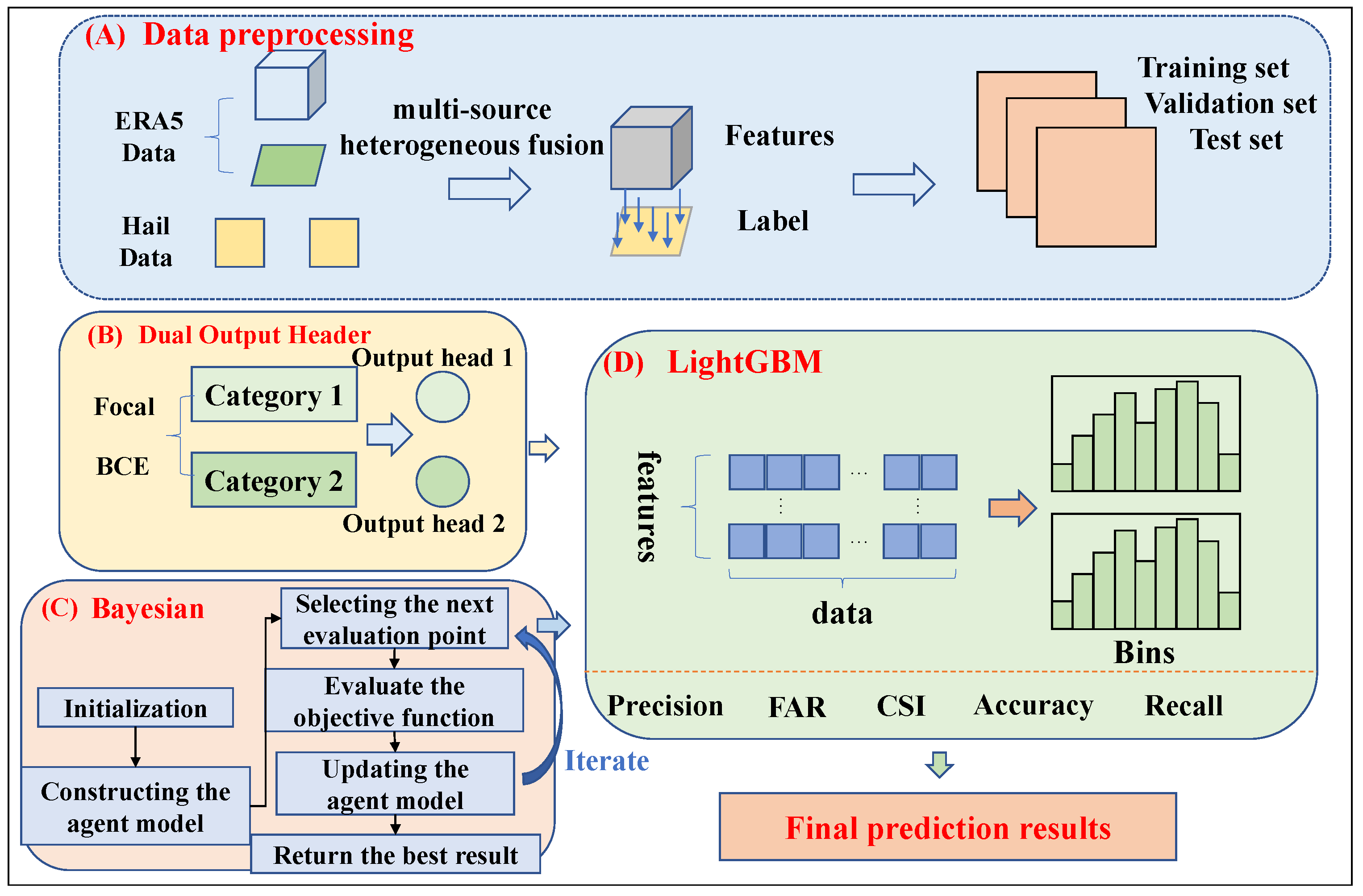
Figure 2.
Data preprocessing process based on a multi-source heterogeneous data fusion method.
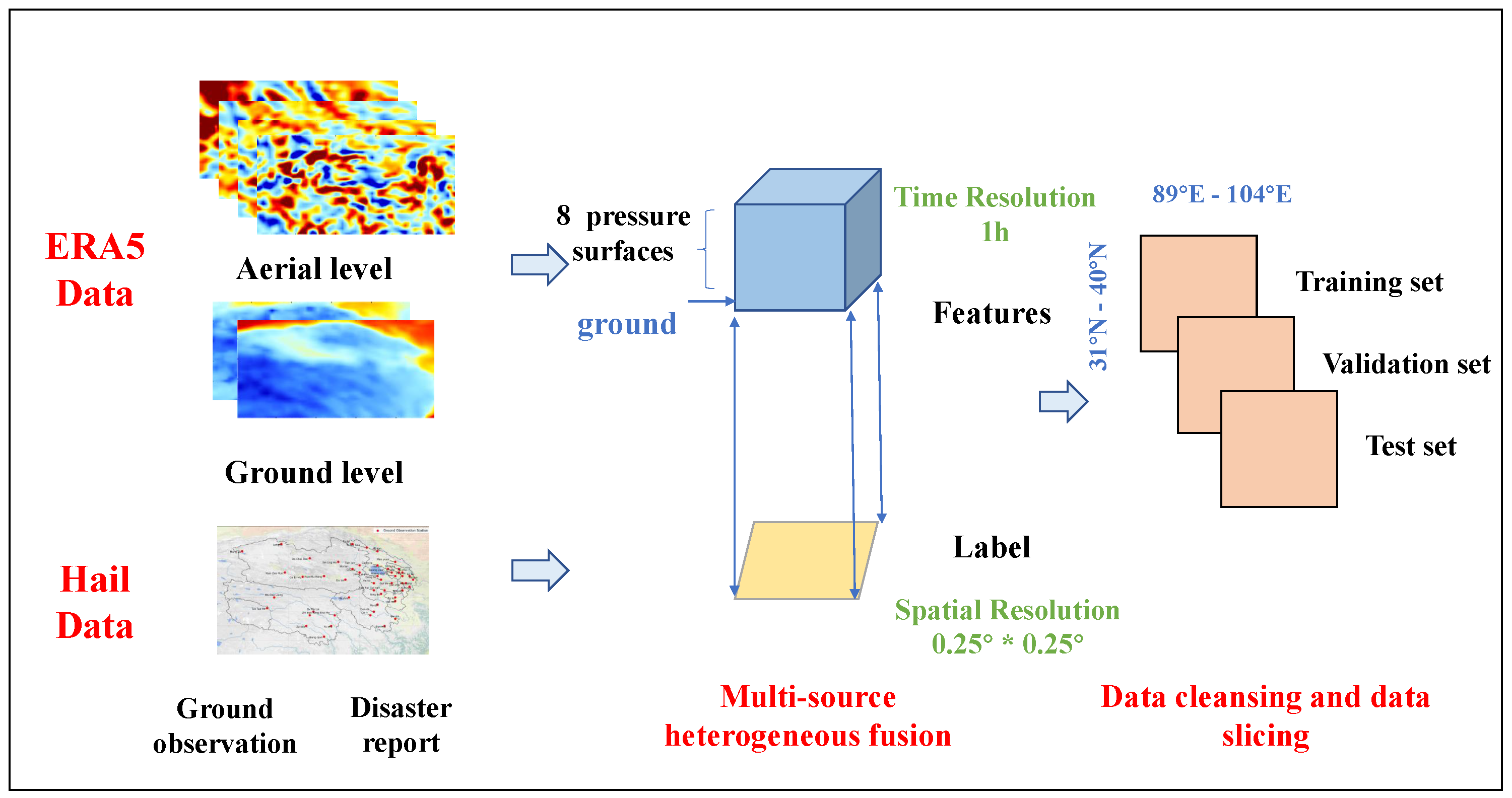
Figure 3.
Schematic illustration of the GBDT algorithm workflow.
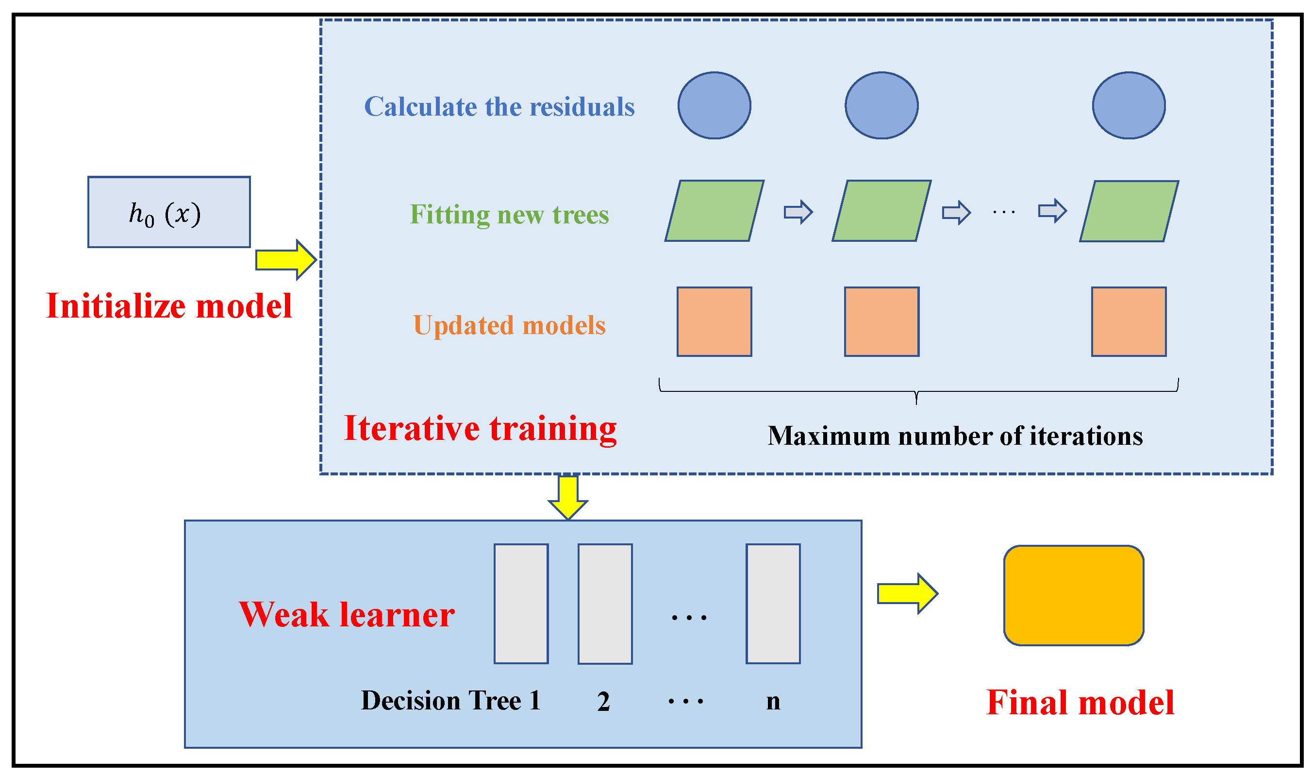
Figure 4.
Key Techniques of LightGBM: GOSS and EFB.
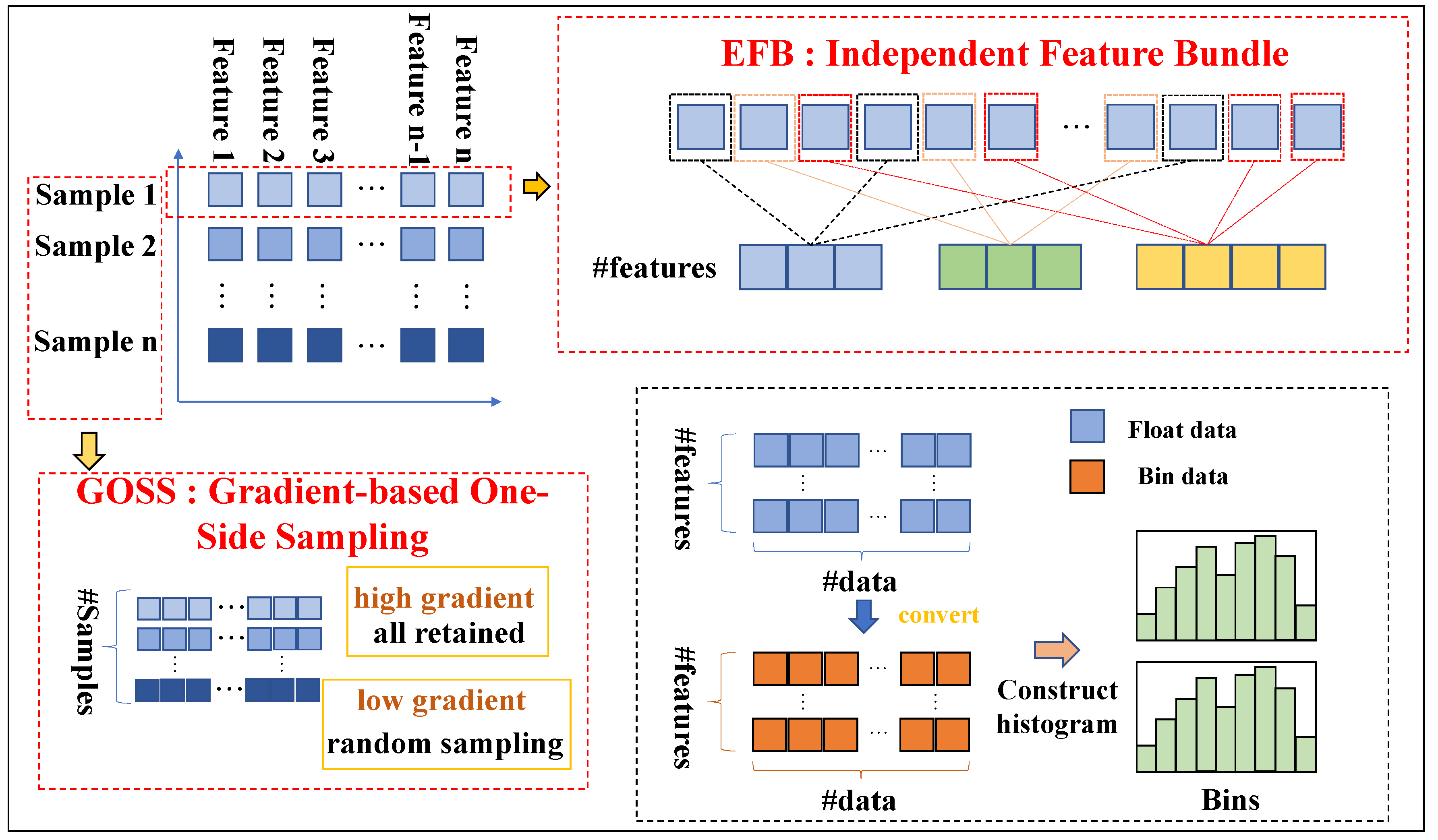
Figure 5.
ROC curves for different Alpha (weighting factor ) and Gamma (modulation factor ) combinations
Figure 5.
ROC curves for different Alpha (weighting factor ) and Gamma (modulation factor ) combinations
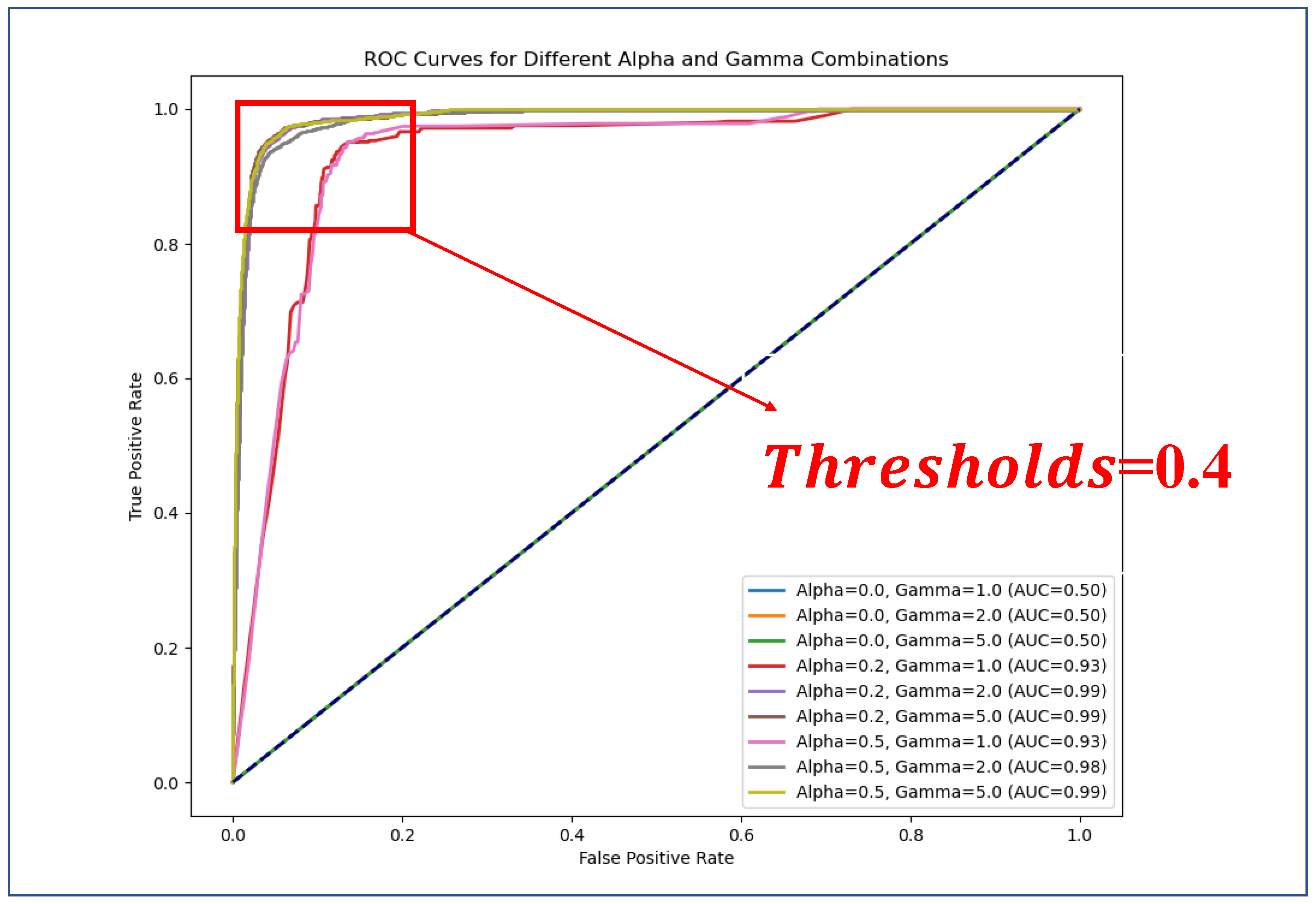
Figure 6.
Accuracy, hit rate and F1-score of the model for different values when =0.4(left), and accuracy, hit rate and F1-score for different values when =2.75 (right)
Figure 6.
Accuracy, hit rate and F1-score of the model for different values when =0.4(left), and accuracy, hit rate and F1-score for different values when =2.75 (right)
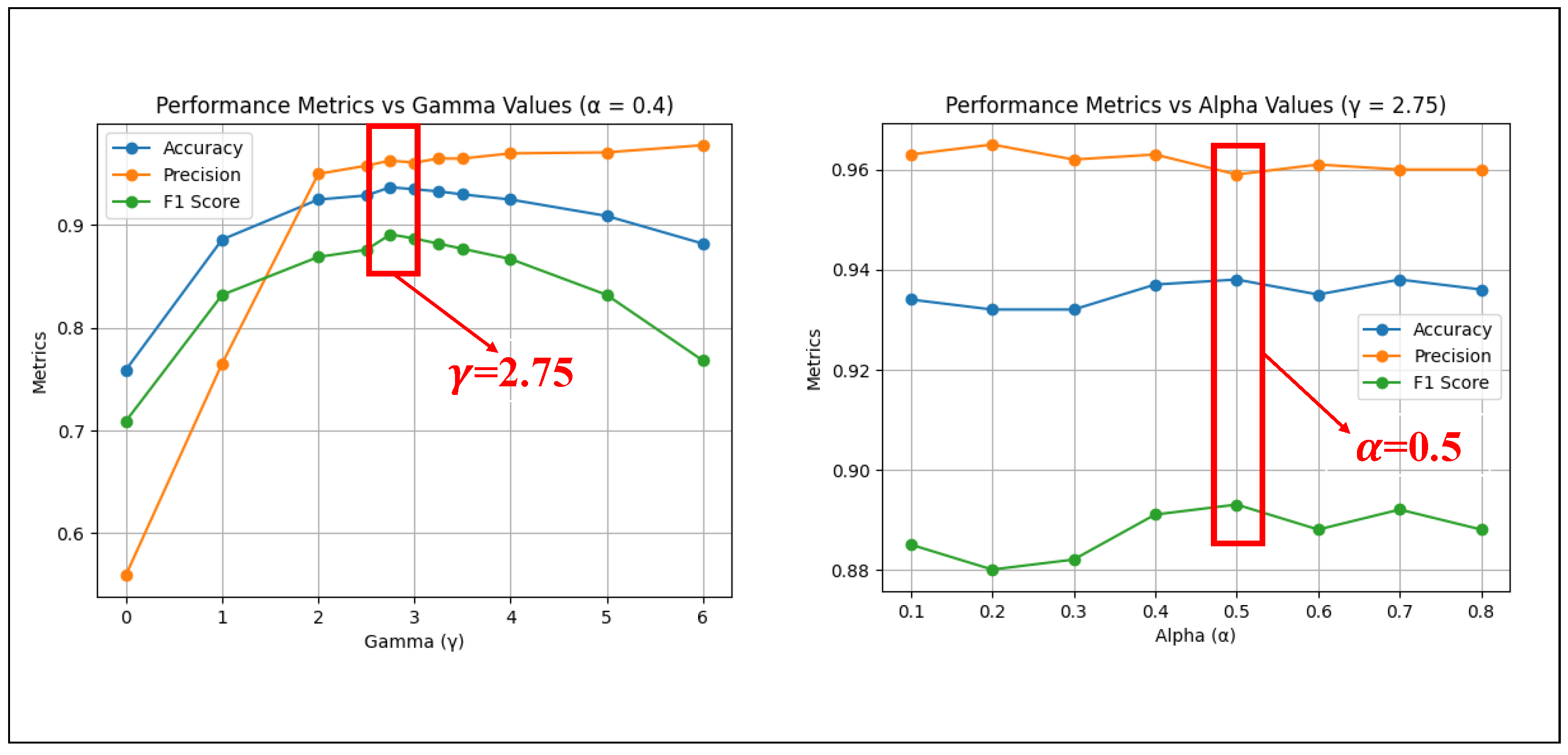
Figure 7.
Confusion matrices of test set predictions for LightGBM and Bayesian-DOH-LightGBM models
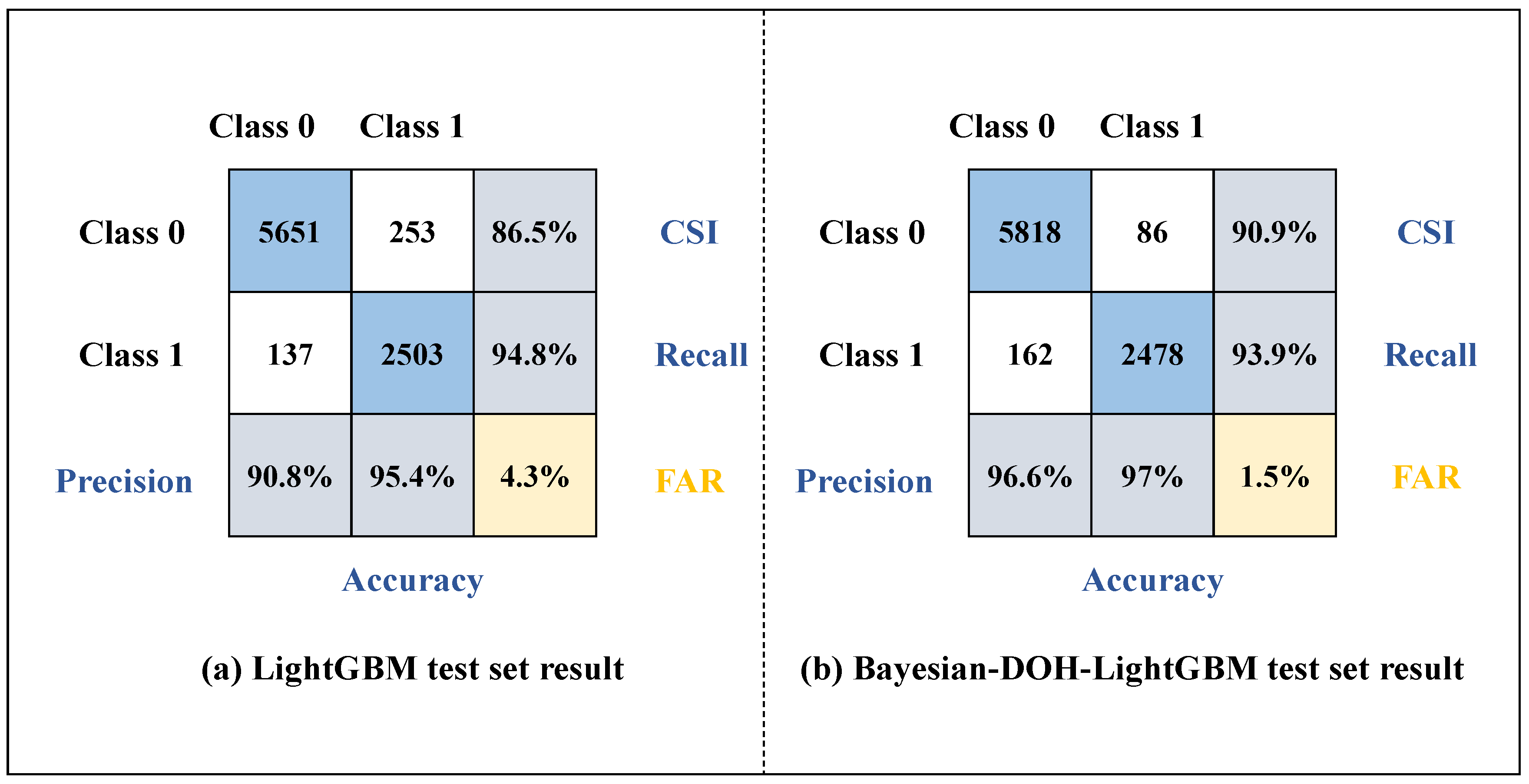
Figure 8.
Top Ten Features Ranked by SHAP Values
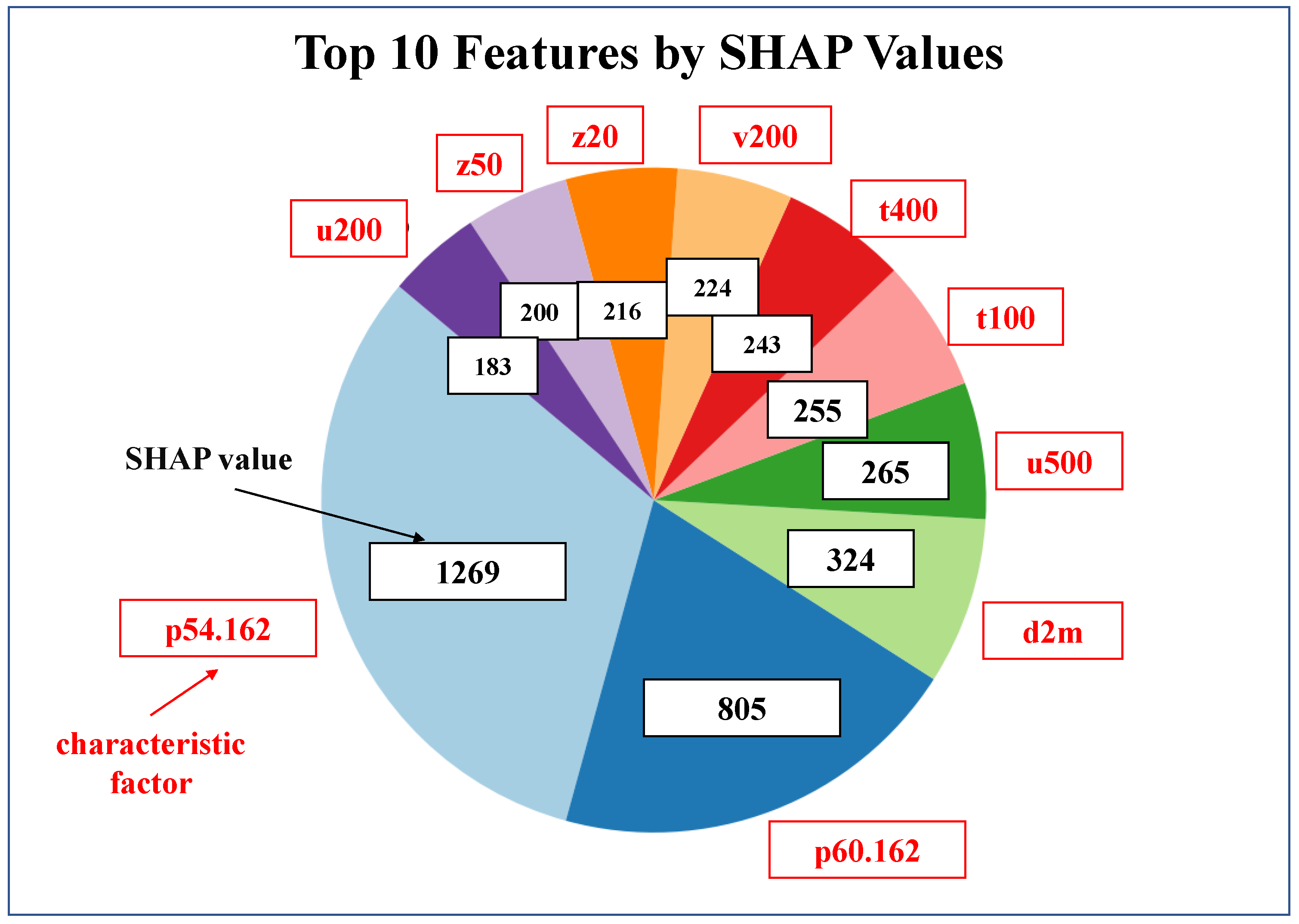
Figure 9.
Kernel Density Estimation Curves of p54.162, p60.162, d2m, t100, u500, and z20.


Table 1.
Distribution of Hail and Non-Hail Samples in Each Dataset.
| Dataset | Year Range | Number of Hail Samples | Number of Non-Hail Samples |
|---|---|---|---|
| Training Set | 2009-2021 | 57384 | 73164 |
| Validation Set | 2022 | 3120 | 5842 |
| Test Set | 2023 | 2640 | 5904 |
Table 2.
Comparison of the prediction effects of LightGBM models with four different output heads.
| Output Head(s) | Accuracy↑ | Precision↑ | F1-score↑ |
|---|---|---|---|
| Single-Focal | 0.955 | 0.908 | 0.929 |
| Single-BCE | 0.938 | 0.959 | 0.893 |
| FB | 0.925 | 0.916 | 0.874 |
| BF | 0.970 | 0.968 | 0.951 |
Table 3.
Experimental results of the three optimization algorithms on the Wine Dataset (a) and the Hail Dataset Subset (b).
Table 3.
Experimental results of the three optimization algorithms on the Wine Dataset (a) and the Hail Dataset Subset (b).
| Method | (a) Wine Dataset | (b) Hail Data Subset | ||
|---|---|---|---|---|
| Evaluation Metrics | Computation Time (s)↓ | Accuracy↑ | Computation Time (s)↓ | Accuracy↑ |
| Random Search | 8.52 | 0.972 | 17.21 | 0.861 |
| Grid Search | 73.19 | 0.972 | 112 | 0.845 |
| Bayesian Optimization | 6.84 | 0.985 | 12.13 | 0.886 |
Table 4.
Optimal parameters of the DOH-LightGBM model obtained using a Bayesian optimization algorithm.
Table 4.
Optimal parameters of the DOH-LightGBM model obtained using a Bayesian optimization algorithm.
| Parameters | BCE Output Header | FOC Output Header |
|---|---|---|
| Num-leaves | 481 | 968 |
| Learning-rate | 0.115 | 0.014 |
| Feature-fraction | 0.870 | 0.869 |
| Bagging-fraction | 0.718 | 0.960 |
| Bagging-freq | 4 | 8 |
| Lambda-l1 | 1.73 | 1.04 |
| Lambda-l2 | 5.96 | 0.896 |
Table 5.
Comparison of experimental results between the Bayesian-DOH-LightGBM model and other mainstream classification models.
Table 5.
Comparison of experimental results between the Bayesian-DOH-LightGBM model and other mainstream classification models.
| Method | Precision↑ | FAR↓ | CSI↑ | Accuracy↑ | Recall↑ |
|---|---|---|---|---|---|
| Decision Tree | 0.909 | 0.033 | 0.690 | 0.897 | 0.741 |
| Random Forest | 0.885 | 0.047 | 0.742 | 0.912 | 0.821 |
| KNN | 0.427 | 0.350 | 0.328 | 0.629 | 0.585 |
| XGBoost | 0.912 | 0.040 | 0.856 | 0.951 | 0.933 |
| AdaBoost | 0.741 | 0.137 | 0.676 | 0.869 | 0.885 |
| LightGBM | 0.908 | 0.043 | 0.865 | 0.954 | 0.948 |
| Bayesian-LightGBM | 0.927 | 0.032 | 0.874 | 0.958 | 0.938 |
| Bayesian-DOH-LightGBM | 0.966 | 0.015 | 0.909 | 0.970 | 0.939 |
Disclaimer/Publisher’s Note: The statements, opinions and data contained in all publications are solely those of the individual author(s) and contributor(s) and not of MDPI and/or the editor(s). MDPI and/or the editor(s) disclaim responsibility for any injury to people or property resulting from any ideas, methods, instructions or products referred to in the content. |
© 2024 by the authors. Licensee MDPI, Basel, Switzerland. This article is an open access article distributed under the terms and conditions of the Creative Commons Attribution (CC BY) license (http://creativecommons.org/licenses/by/4.0/).
Copyright: This open access article is published under a Creative Commons CC BY 4.0 license, which permit the free download, distribution, and reuse, provided that the author and preprint are cited in any reuse.


