
Submitted:
17 December 2024
Posted:
18 December 2024
You are already at the latest version
Abstract
There is now a growing interest in the development of Smart Cities. These cities will provide ubiquitous communication, intelligent transport systems, advanced digital health platforms and urban and infrastructure management. Intelligent Transport Systems will be realised through the emergence and deployment of Satellite Navigation Systems, Vehicular Networking and Connected and Autonomous Vehicles, and should result in less congestion, shorter journey times and a significantly reduced number of road deaths. These new systems allow much more information about vehicles in transit to become available in real-time, including the source and destination of a journey, measurements from vehicles, and the state of the road infrastructure. Such detailed information will allow better analysis of journeys and routes. What is needed are new analytical models to use this information to build more accurate journey times. This paper addresses these issues. A journey is defined as the traversal of several road links and junctions from the source to the destination. The delay at junctions is analysed using the Zero-Server Markov Chain technique. This is then combined with the Jackson Network to analyse the delay across multiple junctions. The delay on road links is analysed using an M/M/K/K model. This approach was used to analyse a real scenario, and the results were validated using a SUMO simulation. The increased accuracy of this model will lead to much better traffic congestion algorithms for Intelligent Transport Systems for Smart Cities.
Keywords:
Intelligent Transport System
; Vehicular Networks
; Calculation of Journey Times
; Zero-Server Markov Chain
1. Introduction
The Smart City agenda is now being pursued by numerous companies, institutions and governments because of the huge societal impact it will have [1]. Intelligent Transport Systems (ITS) is therefore a major component of Smart Cities because they should result in reduced journey times, less traffic congestion and a significant reduction in road deaths which will greatly improve the quality of life of its citizens [2]. ITS will be brought about by the fusion of communication and transport infrastructures to create city-wide vehicular networks that form digital ring roads around the city. These systems will support several networking technologies including 5G, ITS-G5, and future technologies such as IEEE 802.11bd and 6G.
Though we now have several experimental vehicular testbeds [3], in order to build an efficient ITS, it is necessary to develop better traffic management algorithms that will lead to reduced journey times and less traffic congestion. Thus, new techniques are required to analyse journey times in detail. This is the focus of this paper. In the solution approach, a journey is defined as the traversal of junctions and links. A technique called the Zero Server Markov Chain (ZSMC) is used to analyse delays at a junction. This is then combined with the Jackson Network technique to analyse the delays at multiple junctions. The delay along road links is analysed using an M/M/K/K model. A SUMO simulation is then used to compare results while traversing three junctions. The results were compared with SUMO for the same scenario and showed an excellent comparison. Using this approach, Dijkstra’s algorithm is then used to analyse the different routes between a source and a destination to determine the best route [4].
The contributions of this paper can be summarised below:
- A journey is defined as a traversal of junctions and links rather than a traversal of compound links.
- A technique called the Zero-Server Markov Chain (ZSMC) is used to analyse delays at the junction.
- An M/M/K/K model is used to analyse delays along the links.
- An analysis showing how the delay for a route containing 3 junctions and 2 links is demonstrated.
- An analysis of a real scenario is done using Dijkstra’s algorithm and the new techniques.
The rest of the paper is organized as follows: In Section 2, an overview of related work is detailed while Section 3 explains the Zero Server Markov Chain. Section 4 examines the solution approach and highlights the analysis of delays at junctions. Section 5 develops the Markov Chain to analyse the delay along road links while in Section 6 an analysis of three junctions is presented. In Section 7, SUMO is used to evaluate the analysis and Section 8 examines a real-life journey to determine the shortest route. The paper concludes in Section 9.
2. Related Work
2.1. Current Transportation Management System
Transport in urban areas is largely managed by placing sensors and actuators in the road infrastructure. For example, the Split Cycle Offset Optimisation Technique (SCOOT) [5] is a real-time adaptive traffic control system for coordinating and controlling traffic signals across an urban road network. Recently, these systems have been augmented with video and cheaper display technology. With the widespread deployment of the Global Positioning System (GPS), Floating Car Data (FCD), which records the location and mobility of vehicles, is now used by Google and Tom-Tom systems to warn drivers about possible congestion on their route [6].
2.2. Vehicular Networks
The emergence of Vehicular Ad-Hoc Networks (VANETs) that are deployed using Roadside Units (RSUs) along the road infrastructure and Onboard Units (OBUs) in vehicles represents another significant change. Information about vehicles, including their location, speed and state of the vehicle, as well as the source and destination of their journeys, are provided in real-time, allowing new traffic management algorithms to be developed [7]. A VANET network is shown in Figure 1.
2.3. Research Methodology in Transport Research
2.3.1. Work on Testbeds
The development of vehicular testbeds with V2X communications [8] has played a significant part in the development of ITS. The authors in [9] developed a vehicular testbed to explore the communication dynamics of vehicular systems to understand how to provide seamless connectivity in these highly mobile environments by analysing the Network Dwell Time. The results showed that network connectivity was related to frequency and length of the beacon from the Roadside Units (RSUs) as well as the velocity of the vehicle. A key use of these testbeds was to provide realistic input parameters to simulations.
2.3.2. Use of Simulation
Simulation has also been used extensively in transport research. In [10], the authors used two simulators to integrate road traffic data and network communications. These were SUMO and Network Simulator (NS3) for testing the VANET protocol. NS3 can support a large set of simulation scenarios where the number of nodes can be up to 20,000, thus making the simulation results more realistic. In recent years, simulation technology has played a very important role in VANET research. The authors in [11] tried to integrate real vehicle traces into simulation systems. Data was imported from real maps and vehicle traces were restricted to road topology. In this case, the origin and destination of each journey were randomly generated. The authors could not address the traffic problems dynamically in the simulator, and therefore focused on two aspects. The first was to develop a protocol for communication between NS3 and SUMO and the second was the wireless routing protocol and its effect on vehicular travel [10].
2.3.3. Analytical Models
There has been an increased use of Queuing Theory [12,13] to give better performance analysis of emerging networks. In [14], the authors used M/M/K models to analyse SDN networks where routes could be dynamically allocated to help meet Quality of Service (QoS) requirements as the network traffic changes. The findings showed that this approach resulted in increased network utilisation. Furthermore, this approach can also be applied to traffic models in transportation systems. However, the authors analysed the delay along links, using M/M/1/K techniques; their work did not look at the delays at the junctions.
2.3.4. ML and AI in Traffic Management
Increasingly, we are seeing the use of ML and AI techniques in traffic management [15]. Several genetic algorithms, which are discussed below, have been developed to reduce traffic congestion and shorten journey times.
2.4. Current Analysis of Journey Times
In [16] [1] the authors considered an adaptive genetic algorithm for reducing the average waiting time at the traffic light. In this work, they used SUMO for the implementation. The genetic algorithm required a number of iterations and hence there are issues around scalability and its use in real time systems. In [17] [2] the authors looked at improving Dijkstra Algorithm for vehicular routes in urban areas, in which two different Dijkstra systems are combined: the first is for distance and the second is for traffic. This method was used between two paths and there are scalability issues for heavy traffic systems. In [18] [3] the authors looked at how we can use VANET network traffic to predict traffic flow on the road. The system uses two algorithms. The first is Random Forest (RF) which is a machine learning algorithm to analyse the network traffic and the second is Gated Recurrent Unit (GRU) algorithm which is a deep learning algorithm to analyse the road traffic. The system did improve the overall traffic, but there are scalability issues and it may not be suitable for real time traffic situations. In [19][4] the authors attempted to analyse and manage the regional traffic flows using a traffic classifier and a genetic algorithm. There are scalability issues but the results could be used to drive a mathematical model. Finally in [20] [5] the authors tried to optimise a multi-junction traffic light control system using a genetic algorithm and by classifying the traffic as either light, medium, heavy and very heavy. The algorithm shows improvement but cannot adapt to the changing nature of traffic. A summary of these systems is shown below in Figure 2
2.5. Research Gap
As shown above, all the models presented had issues relating to scalability, performance and use in real time systems. In contrast, our approach is to use new analytical models based on queuing theory to analyse individual journeys using real time readings from the Transport Network such as the Middlesex VANET Testbed. In particular, this work will give a highly accurate model using a new Zero Server Markov Chain (ZSMC) technique to determine the delays at the junction. We know this approach should be effective as it was used to analyse Intelligent Service Migration in vehicular networks [21] in which vehicles are handing over to different Road-Side Units (RSUs) and hence service is not available during handover. In our work, we are trying to get a detailed picture of the delays at the traffic light/ junction in which when the light is red, service is not available because the vehicle cannot proceed and when it is green, the service is available because the vehicle can proceed. Hence, the ZSMC technique can be used to give a detailed analysis of the delays at the junction. Previously, delays at junctions were estimated using large datasets [22] but this new approach should provide much greater accuracy. We will also look at an M/M/K/K queuing model to analyse the links between junctions. Finally we will combine this with the Jackson Network technique and Dijkstra Algorithm [23] to find the delays from source to destination. Our approach [6] is also summarised in Figure 2.
3. The Zero-Server Markov Chain
Markov Chains which use the concept of arrival and service rates can be applied to yield steady state system probabilities. However, though an ordinary Markov chain can be used to analyse when the client can communicate with the server, in mobile environments, a new type of Markov must be used to analyse the system as the server will not always be available. Thus a Zero-Server Markov Chain (ZSMC) in which only arrivals occur as shown in Figure 3 must be employed to deal with these situations.
A Zero-Server Markov Chain is inherently unstable because after long time the length of the queue will go to infinity. In order for the system to become stable, the ZSMC must be coupled with another Service-Based Markov Chain (SBMC) which serves customers/packets allowing them to leave the system. Thus the system must be represented by two chains, the ZSMC and the SBMC. The state of the system is given by N,M where N is the number of requests and M is the number of servers. For the ZSMC, M is zero so the state is given by N, 0 with probability . An example of an SBMC is an exhaustive service model in which when the server arrives at the queue, it serves exhaustively until there is no on left in the queue before it moves to the other queues. This is explored fully in [24].
Figure 4 shows the situation when the server does not serve exhaustively. The symbols are explained in Table 1.
Using Steady State Markov Chain Analysis we get the following results:
3.1. Handling a System with Capacity K
3.2. New Concept: Lost Service
In this section we introduce the concept of lost service which occurs when there are customers at queue to be served by the server is not available. This is expressed as the probability of any customers being in the Zero Server Markov Chain. Hence is the sum of P(N,0) where N goes from 1 to ∞ or from 1 to K, where K is the capacity of the system. Lost Service is therefore a new parameter that measures the effect of the server not being at the queue in cyclic queuing systems.
4. Summary of Previous Work
In this section, we briefly summarise the previous work done in [25].
4.1. Journey Analysis
A journey is defined as the need to traverse a series of links (M) and a number of junctions (N). The denotations are as follows:
- A Journey is given by JO(i)
- A link is given by (Li)
- A junction is given by (Ji)
Thus we can now write that the time for journey as:
4.2. Analysis of Delays at Junctions
In order to analyse the delay at the junction, we use the Zero Server Markov Chain (ZSMC) technique described above. In this case, we are considering when the traffic light is green, vehicles can move forward at the junction and hence are served by the junction. Hence, when the light is green, this can be viewed as the situation when the server is at the queue serving its customers because when the light is green vehicles can travel across the junction. However when the traffic light is red, vehicles cannot proceed past the junction because the service is not available at the time. Thus the situation of the junction can be modelled using a Zero Server Markov Chain. Hence, the parameters are:
= Arrival rate of vehicles to the Junction
= Service rate of vehicles traversing the Junction
= (1/T) (Green Signal to Red Signal)
= (1/T) (Red Signal to Green Signal)
4.3. The Analysis of One Junction
Initially the results were carried out for one junction on a weekday in the city of Leicester, UK. It was at the Thurmaston Roundabout where the vehicles were moving in all directions. The start time was 6:00 am in the morning and the calculation of the vehicles was started. Firstly, results were observed for the total numbers of cars that turned left, the total number of cars that turned right and the total number of cars that went straight ahead. At the junction exits, the total number of cars exiting the junction was calculated. These input values were obtained every minute for 15 minutes and then used to calculate the arrival rate of the vehicles along each lane going into the junction. Thereafter these values were used as input to Equations (1) and (2).
4.4. Scenario 1: Turning Left
The arrival rate is calculated in order to check how many cars are turning left on the junction. For different scenarios, the service rate changes. The service rate will be given as where T is the time for the vehicle to turn left at the junction. The time T was set to 3 seconds.
4.5. Scenario 2: Going Straight
In the second scenario the cars considered are the ones moving straight ahead on the junction. Again 06:00 hours was the start time. Data was obtained every minute as to how many vehicles were going straight ahead. Data was updated at the end of fifteen minutes. Once the data was updated at the end of fifteen minutes, values were calculated in seconds. The service rate to go straight on will be given as be given as .
4.6. Scenario 3: Turning Right
In the third scenario the cars will be turning right on the junction. Time slots and duration etc. are considered the same as in previous scenario. The service rate to leave the third exit or to turn right will be given as 1/(3*T).
Figure 5 shows the graph of one junction where on the X-axis it is number of vehicles approaching the junction or the capacity of the system, K, within the area. The Y-axis shows the Average Response time for cars turning left, going straight and turning right. The results show that turning left is quickest and turning right has the largest response time as it takes the more time to turn right. What is surprising that only a small value of K is needed to achieve the maximum response time and hence the maximum throughput is quickly achieved after which there is minimal effect in increasing K.
4.7. Analysis of the Two-Junction Scenarios
In this section, the technique used above is extended to look at two-junction scenarios.
4.8. Jackson Network Analysis
The Jackson network technique allows us to explore delays at multiple junctions because the technique states that the input rate into the junction is equal to the output rate of the previous junction. Hence for a two-junction system, the input rate of traffic into the second junction is equal to the output rate of the first junction [26].
After using the ZSMC technique for a single junction, we combine this with the Jackson network model to explore the delay at multiple junctions. Once the values have been captured from the exit of the first junction using the ZSMC model, it is possible to use the Jackson network model to obtain results for multiple junctions. This can be used to find the delays along routes from source to destination.
Figure 6 shows the resultant graph for two junctions where on the X-axis it is the number of vehicles approaching the junction within the area, and on the Y-axis is the Average Response time for vehicles turning left, going straight and turning right which is the time taken to travel along two junctions. These results show that there are further delays going through the two junctions, but the overall observation is similar to that obtained at junction 1; but the slope of the initial sections are steeper and longer for the two junction scenario. This points to a greater variation of delay for the two junctions compared to the single junction.
5. Analysing the Delay Along the Road Using a Markov Model
In this section, we develop a Markov Model to calculate the delay along the road links.
Let the length of the road = L(Road)
Length of the vehicle = L (VEH)
The capacity of the road is K (Road) which is the total number of cars that can be travelling on the road at the same time.
Hence K(Road) is given by:
However, K vehicles can travel along the road at the same time. Thus, K vehicles can be served simultaneously. Hence the road has K servers, so this is an M/M/K/K Model. Hence, we can represent this by the Markov Chain shown in Figure 7.
Applying Markov Balance for States 0, 1, 2, and 3 we get the general equation:
Thus, we sum the probabilities to get the value of and then we obtain the average number of customers/vehicles in the system as well as the response time of the vehicles in the system given by T(VEH).
5.1. Understanding The System Time Parameter
For the Jackson network, we need to also express the System Time T(SYS) which is the Time as seen by someone measuring the time at which vehicles are leaving the road. Since there are K servers, thus K vehicles can be served simultaneously. Hence, this time is given by:
A simple C program was used to calculate these values for different arrival times and service rates as well as the capacity of the road.
This scenario is shown in Figure 8
5.2. Analysis of Second Junction with Inter Connecting Links
In this section we consider the scenario of two junctions separated by the road examined above. In this case the rate of arrival into the second junction from the road is equal to the inverse of sum of the Response Time at Junction 1 and the Time along the Road.
= 1 / ( 22.677 + 0.3636 )
= 1/23.0406
= 0.0434
5.3. Getting a Proper Estimate of K For Second Junction
For the calculation of delay at second junction we need to get an effective value of K. We know that K has maximum value which is maximum number of cars that can traverse on the road is 500. However we can use our model of the link to get a realistic value of K. From our model, M/M/K/K model, the average number of vehicles on the road was 7.99, therefore we can use values of K between 1 and 15.
6. Three Junction Scenarios
The scenario being considered is on a weekday in the city of Leicester, UK and was at the Thurmaston roundabout as well as the Melton Road A607 Roundabout where the vehicles were moving in all directions. The start time was 6:00 am in the morning and the calculation of the vehicles was started. The setup is shown in Figure 9.
The model for this scenario is shown in Figure 10. In the previous section, we considered Junction 1 and Junction 2 connected via road and link and showed how we calculated the delay in such system. In this section, we will extend the work to consider a three junction scenario and hence we introduce Junction 3 as well as the second link between Junction 2 and Junction 3 shown in Figure 11.
Therefore we now calculate the delay on the road between junction 2 and junction 3.
VMAX Speed = 40 kilometres/hour
L (Road) = 2500 metres between junction 2 and junction 3
The value of T(Road)is given as
T(Road) = 225 Seconds
Therefore the service rate per vehicle is given by:
Let K be the capacity of the road link in terms of the number of vehicles fit in road.
The value of K = 625
The arrival rate of the vehicles going from junction 2 to junction 3 is given by
Using the algorithm to calculate the delay on the road we get:
Average number of Vehicle on the road = 3.288
Average time to traverse the road is = 225.225 seconds
Average Response time for the system = 0.3603seconds.
Blocking Probability = 0
6.1. To Find the Delay at Third Junction
To calculate the delay at third junction we say that rate into Junction 3 is given by:
= Rate of going straight on Third Junction
= 0.1667
K= 15
= 1 / (22.677+0.3636+45.208+0.3603)
= 0.01457
6.2. Finding the Actual Journey Time
To find the actual journey time between source and destination we need to find the exact time that the vehicle takes to travel along the link as well as the time it takes to navigate the junctions. In this scenario the journey time is equal to
Actual Journey Time = (T Junction 1) + (Traversal delay of Link 1) + (T Junction 2) + (Traversal delay of Link 2)+ (T Junction 3)
Actual Journey Time = 22.677+ 181.818 + 45.7577 + 225.225 + 26.657
Actual Journey Time = 501.954 seconds
Therefore the actual journey time from Source to Destination is 501.954 seconds.
6.3. Results of Three Junctions
The results for the 3-junction scenario without links are shown in Figure 12 while the results for 3-junction scenario with links are shown in Figure 13. The results show that the effect of the links is to slow the rate of traffic going unto Junction 3, hence reducing the overall response time through Junction 3. This was similar to the results previously obtained for 2-junction scenario.
7. SUMO
SUMO source forge 2013 highlights the power of SUMO statistics. SUMO has powerful graphics, researchers could benefit more from SUMO which has statistical files in various forms such as output coupled to traffic, which picks from the Traffic Control Interface (TraCI) performance parameters [27,28]. Principles of Highway Engineering, and also congestion analysis describe the following measures as useful for examining traffic navigation algorithms; simulation flow rate is the maximum hourly volume that can pass through an intersection between lanes, if that lane was allocated constant green light over the course of an hour.
Lost Time is the portion of the cycle length that is not being completely utilised. In other terms, because the traffic light alternates the right-of-way between conflicting movements, where traffic flows are continuously started and stopped. Every time this happens there is a lag due to drivers reacting to the change of traffic light signal. This lag at the beginning and the end of green and yellow signal interval results in a portion of that interval to not be completely utilised. This lag is known as lost time. SUMO is a car following model based on the Dijkstra, 1972 algorithm and random walk for its path modelling. The input parameters below were used in the SUMO simulation.
Length of car : 4 metres
Junction Type : Three-Junction Scenario
Vehicle Type: Car
Vehicle Colour : Yellow
Traffic Signal Time : 0.05 seconds
Each Lane has a Unique Id to show the cars travelling in that lane. SUMO creates the trips on its own by editing the parameters. Once the trips are calculated then it will run the simulation. Once the simulation is run as seen in Figure 14, the vehicles are moved along the journey from Point A to Point B. This simulation supports two-way traffic flow. Hence it can start from any direction. The simulation ran for 503 seconds and was then stopped to show that all vehicles in the system, have completed their journey.
The result from the SUMO simulation to go from Junction 1 to Junction 3 is 500 seconds while the results from using analytical modelling was 501.954 seconds. Hence the results validate the approach taken in this work. Therefore when comparing the analytical and simulation model the results are approximately the same.
8. Analysing Real Journeys
In this section, we look at a journey shown in Figure 15. There are three different routes to the destination and the algorithms developed in the previous sections are now used to calculate the delays along the different routes to determine which is the shortest route for the journey.
8.1. Route 1
Route 1 : Green Colour:
Route 1 starts from Source A to Junction 1 and then there is a separate route leading straight to the Destination
Journey time along the common route is 36 seconds.
The time to go across Junction 1 is 22.67 seconds.
The time to go along the road to the destination is 724.6376 seconds.
The total time for Route 1 is 783.3076 seconds.
8.2. Route 2
Route 2 : Black Colour :
Route 2 starts from Source A to Junction 1 and then proceeds to Junction 2 and then from there is a direct route to the Destination.
Journey time along the common route is 36 seconds.
The time to turn right on Junction 1 is 30.67 seconds.
The time to traverse the link from Junction1 to Junction 2 is 181.81 seconds.
The time to go across Junction 2 is 29.500 seconds.
The time to go along the road to the destination is 480.769 seconds.
The total time for Route 2 is 758.0871 seconds.
8.3. Route 3
Route 3 : Orange Colour
Route 3 starts from Source A to Junction 1, then through Junctions 2 and 3 and then we get a road to the Destination.
Journey time along the common route is 36 seconds.
The time to turn right on Junction 1 is 30.67 seconds.
The time to traverse the link from Junction1 to Junction 2 is 181.81 seconds.
The time at Junction 2 is 35.8073 seconds.
The time to go along the link from Junction 2 to Junction 3 is 227.2727 seconds.
The time to traverse Junction 3 is 17.5756 seconds.
The time taken to go on the road to the final destination is 240.3846 seconds.
The total time along Route 3 is 769.5277 seconds.
8.4. Final Results
The final results are shown is Table 2.
9. Conclusions and Future Work
This paper has explored new techniques for calculating journey times by first representing a journey as a traversal of links and junctions. The analysis of the junction was done using the Zero-Server Markov Chain technique while the analysis of links was done using a M/M/K/K model. These techniques were combined with the Jackson Network technique to analyse journey times in an urban environment. SUMO, an open source vehicular simulator, was used to validate the results which clearly show that there was a close comparison between the simulation and the analytical model. The technique was then applied to a real scenario to calculate the shortest path between source and destination. It is hoped that this new technique will be used in new traffic models to help reduce overall journey time and to reduce traffic congestion on our roads, leading to an improved quality of life for all. This work will allow us to calculate journey times down to seconds which was not really possible with other methods. This approach can also make full use of the data being made available by modern vehicular networks which will allow data on the vehicles to be gathered in real time and hence this method could be used to develop detailed traffic congestion algorithms for real systems. However, though these results are encouraging, a lot more work is needed to make this work useful for transport professionals including addressing the issues of multiple lanes, different types of roundabouts and road topologies as well as issues of scalability and performance. Finally, it is important to develop AI and ML algorithms [29] based on this work and to integrate them into mobile edge environments [30] to support ITS for Smart Cities.
Author Contributions
Queuing Theory Analysis, ZSMC and M/M/K/K Models G.M. SUMO Simulation, Generation and Analysis of Results V.M. Analysis of Results, review V.G. Writing and Editing G.M., V.M. and V.G.
Acknowledgments
This research article is based on the PhD thesis of Dr Vatsal Mehta entitled Developing Traffic Predictions from Source to Destination using Stochastic Modelling, Middlesex University, London, May 2023. Please contact the authors for further details. The authors would like to thank the MDPI Future Internet Team for the opportunity to publish this article and hope that it contributes to the development of Intelligent Transport Systems.
References
- Yang j, Kwon Y and Kim D. ”Regional Smart City Development Focus: The South Korean National Strategic Smart City Program." IEEE Access, vol. 9, pp. 7193-7210, 2021. [CrossRef]
- Koutra Sesil, Becue Vincent and Ioakimidis Christos S. "A Multiscalar Approach for Smart City Planning". 2018 IEEE International Smart Cities Conference (ISC2), pages 1-7, September 2018.bhttps://. [CrossRef]
- Mapp Glenford, Ghosh Arindam, ParanthamanVishnu Vardan, Dohler Mischa and Sardis Frank. "Connected vehicle testbed: development and deployment of C-ITS in the UK". 2018. https://repository.mdx.ac.uk/item/89740.
- Founoun Adnane and Hayar Aawatif. "Evaluation of the concept of the smart city through local regulation and the importance of local initiative". 2018 IEEE International Smart Cities Conference (ISC2), pages 1-6, September, 2018. https://. [CrossRef]
- Department for Transport, United Kingdom. "The SCOOT Urban Traffic Control System". 1995.https://tsrgd.co.uk/pdf/tal/1995/tal-4-95.pdf.
- Cohn, Nick and Bischoff, Hugo. Company TomTom. "Floating Car Data for Transportation Planning". National Travel Monitoring Exposition and Conference, 2012. https://onlinepubs.trb.org/onlinepubs/conferences/2012/NATMEC/Cohn.pdf.
- Schulz W. H, Wieker H and Arnegger B. ”Cooperative, connected and automated mobility,” Future TelcoAnonymous Springer, 2019, pp. 219-229.
- McLellan Charles. "V2X Communication". 2018. https://www.zdnet.com/article/what-is-v2x-communication-creating-connectivity-for-the-autonomous-car-era/. https://doi.org/12/03/2018.
- Ghosh Arindam, Paranthaman Vishnu, Mapp Glenford and Gemikonakli, Orhan. "Exploring efficient seamless handover in VANET systems using network dwell time". EURASIP Journal on Wireless Communications and Networking, pages 1-19. 2014. ISSN 1687-1472. https://. [CrossRef]
- Sha L and Lijun S. "Real-time estimation of traffic retention based on M/G/n/0 queuing model". 2017 Chinese Automation Congress (CAC), pages 6628-6633, October 2017. https://. [CrossRef]
- Kumaran U and Shaji R.S. "Vertical handover in Vehicular ad-hoc network using multiple parameters". International Conference on Control, Instrumentation, Communication and Computational Technologies (ICCICCT), 2014, pages 1059-1064, July 2014. https://. [CrossRef]
- Gross Donald and Harris Carl M. "Fundamentals of Queueing Theory (Wiley Series in Probability and Statistics". February 1998. Wiley-Interscience. ISBN 0471170836.
- Sztrik J. Basic Queueing Theory. Sztrik online, 2012, 2021.
- Thiruvasakan Lakshmi Priya, Vien Quoc-Tuan, Loo Jonathan and Mapp Glenford. "A QoS-Based Flow Assignment for Traffic Engineering in Software-Defined Networks". Advanced Information Networking and Applications, 2020. pages 762-774. Editors Barolli Leonard, Takizawa Makoto, Xhafa Fatos and Enokido Tomoya, Springer International Publishing. ISBN 978-3-030-15032-.
- Garg D, Chli M and G. Vogiatzis. ”Deep reinforcement learning for autonomous traffic light control.” 2018 3rd IEEE International Conference on Intelligent Transportation Engineering (ICITE), 2018, pp. 214-218.
- Sankaranarayanan Manipriya, Yerramsetty Sudhasree, Kakkera Santosh and Kumar Nitant. "Adaptive Genetic Algorithm for Reducing Average Waiting Time for Road Traffic Signals". 5th International Conference on Innovative Trends in Information Technology (ICITIIT), 2024. pages 1-6, March 2024. https://. [CrossRef]
- Utomo Derrick Daniel, Aurelia Maria, Tanasia Steffi Maria, Nurhasanah and Handoyo, Alif Tri. "Implementation of Dijkstra Algorithm in Vehicle Routing to Improve Traffic Issues in Urban Areas". 3rd International Conference on Smart Cities, Automation & Intelligent Computing Systems (ICON-SONICS), 2023, pages 73-78, December 2023. https://. [CrossRef]
- Sepasgozar, Sanaz Shaker and Pierre, Samuel. "Network Traffic Prediction Model Considering Road Traffic Parameters Using Artificial Intelligence Methods in VANET". IEEE Access, 2022, pages 8227-8242, Volume 10. ISSN 2169-3536. https://. [CrossRef]
- Shao Zhengda, Yang Honglu and Yue, Guiyang. "Time-allocation Optimization of Regional Traffic Computer Control Based on Distributed Algorithm". International Conference on Integrated Intelligence and Communication Systems (ICIICS) 2023, pages 1-6, November 2023. https://. [CrossRef]
- Yew Ther Ming, Wong Richard T.K, Jasser Muhammed Basheer, Chua Hui Na, Al-Qasem Al-Hadi and Ismail Ahmed. "Optimization of Multi-Junction Traffic Light Control Using the Classic Genetic Algorithm". IEEE 11th Conference on Systems, Process & Control (ICSPC), 2003, pages 367-372. https:://. [CrossRef]
- Ezenwigbo, Onyekachukwu Augustine. "Exploring intelligent service migration in a highly mobile network". PhD thesis, Middlesex University, 2022.
- Manley, Ed. "Estimating Urban Traffic Patterns through Probabilistic Interconnectivity of Road Network Junctions". PLOS ONE, Public Library of Science, Volume 10, Number 5, pages 1-17, March 2015. https://. [CrossRef]
- Gbadamosi O. A and Aremu D. R. ”Design of a Modified Dijkstra’s Algorithm for finding alternate routes for shortest-path problems with huge costs,” 2020 International Conference in Mathematics, Computer Engineering and Computer Science (ICMCECS), 2020, pages 1-6. [CrossRef]
- Mapp G.E., Thakker D and Gemikonakli, O. "Exploring a new Markov chain model for multi-queue systems". Computer Modelling and Simulation (UKSim), 2010 12th International Conference, pages 592-597. https://. [CrossRef]
- Mehta V, Mapp, Gl and Gandhi V. "Exploring new traffic prediction models to build an intelligent transport system for smart cities". 2022 IEEE/IFIP Network Operations and Management Symposium, NOMS 2022, pages 1-6.
- Alam, Md. G R et al. "Queueing Theory Based Vehicular Traffic Management System Through Jackson Network Model and Optimization". IEEE Access 2021, Volume 9, ISSN 2169-3536. pages 136018-136031. https://. [CrossRef]
- Song H and Min O. "Statistical traffic generation methods for urban traffic simulation". 2018 20th International Conference on Advanced Communication Technology (ICACT), pages 247-250. February 2018. https://. [CrossRef]
- Liu W, Wang X, Zhang W, Yang L and Peng C. "Coordinative simulation with SUMO and NS3 for Vehicular Ad Hoc Networks". 2016 22nd Asia-Pacific Conference on Communications (APCC), August 2016. https://. [CrossRef]
- Cheng Y and Li X. "A compute-intensive service migration strategy based on deep learning algorithm." IEEE 4th Information Technology, Networking, Electronic and Automation Control Conference (ITNEC), pages 1385–1388, 2020.
- Valsamas P, Mamatas L and Contreras L. M. "A Comparative Evaluation of Edge Cloud Virtualization Technologies." IEEE Transactions on Network and Service Management 19, 2 pages 1351–1365, 2022. https://. [CrossRef]
Figure 1.
A VANET Network.
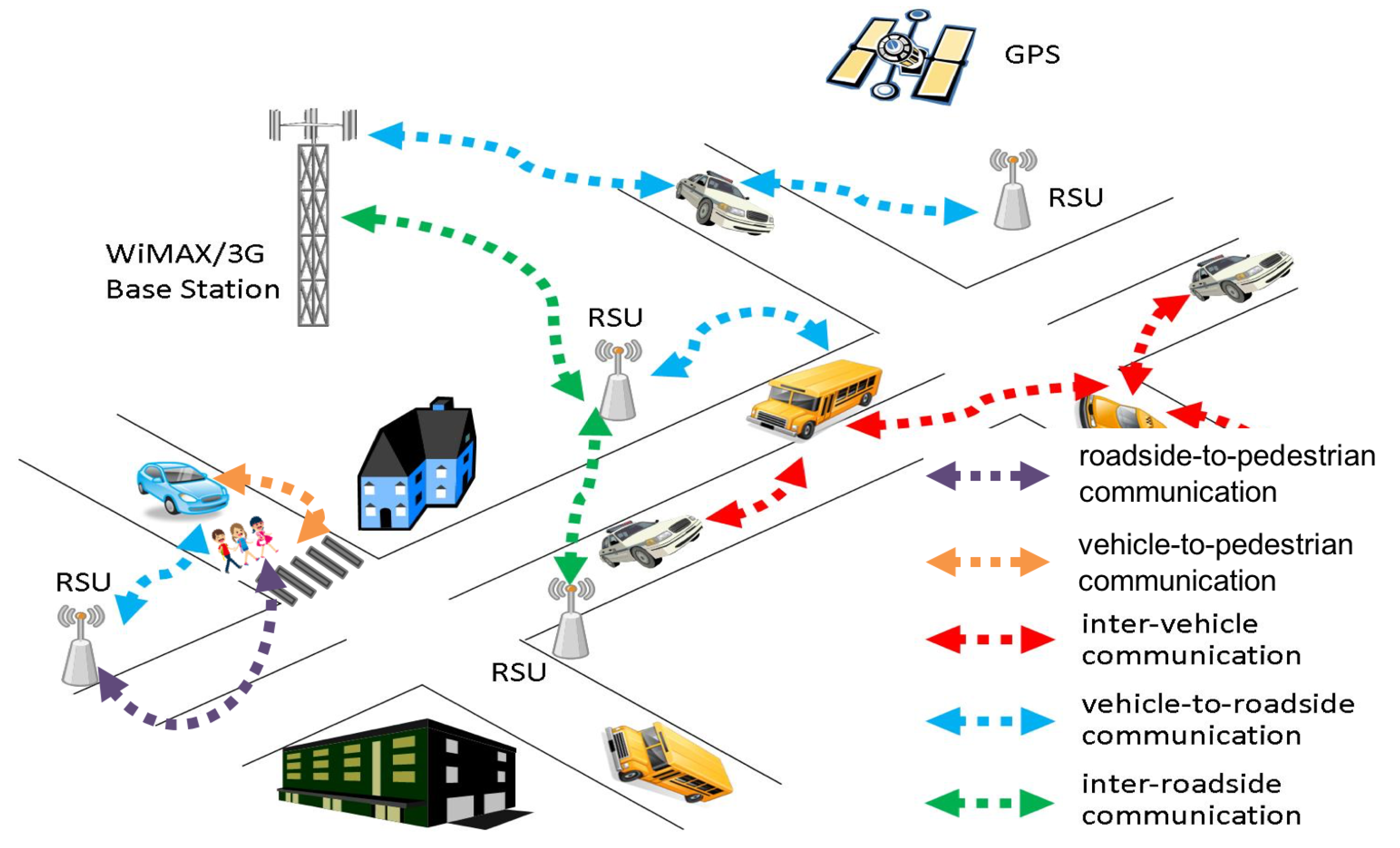
Figure 2.
Current Analysis of Journey Times.
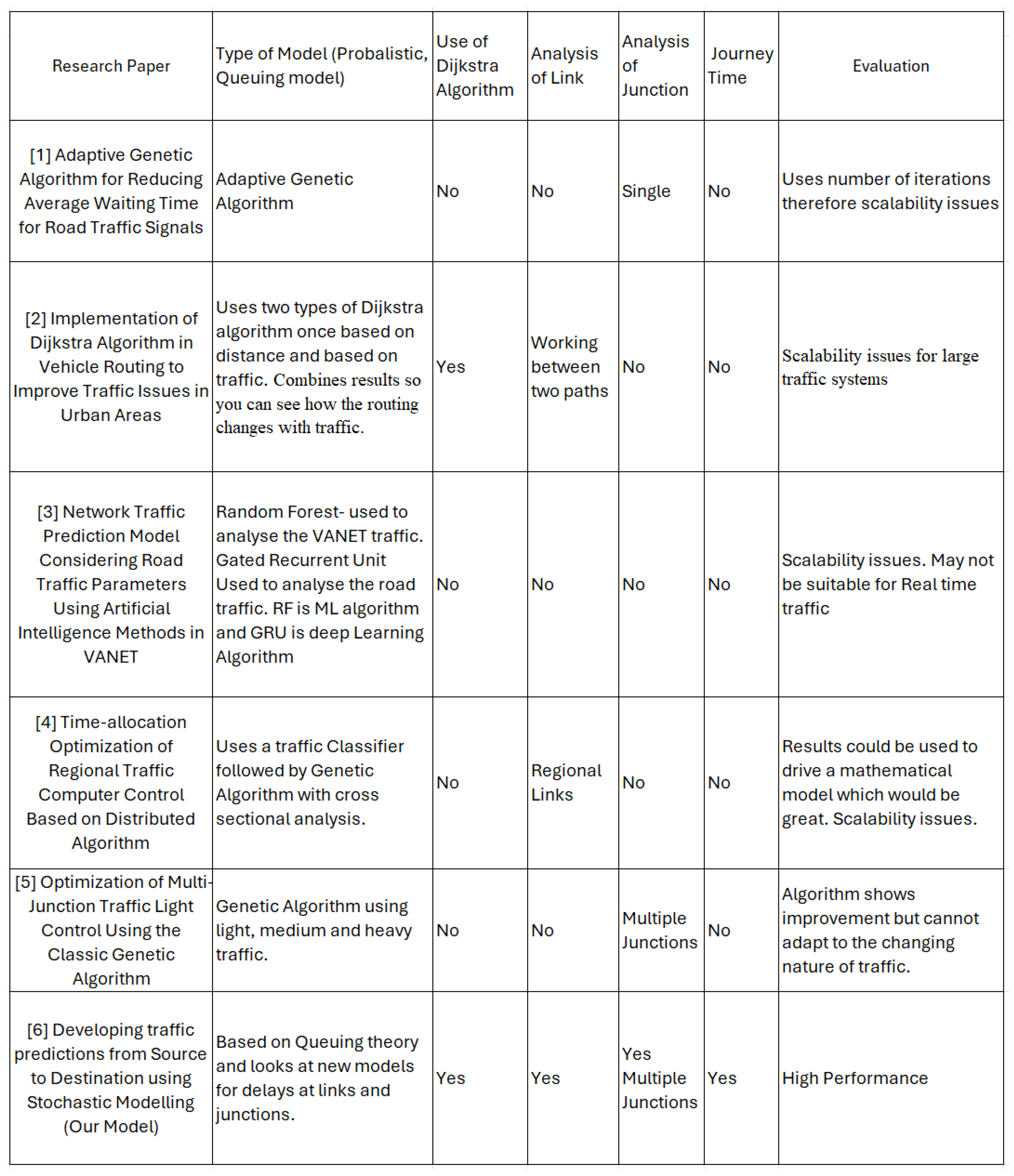
Figure 3.
A Zero-Server Markov Chain.
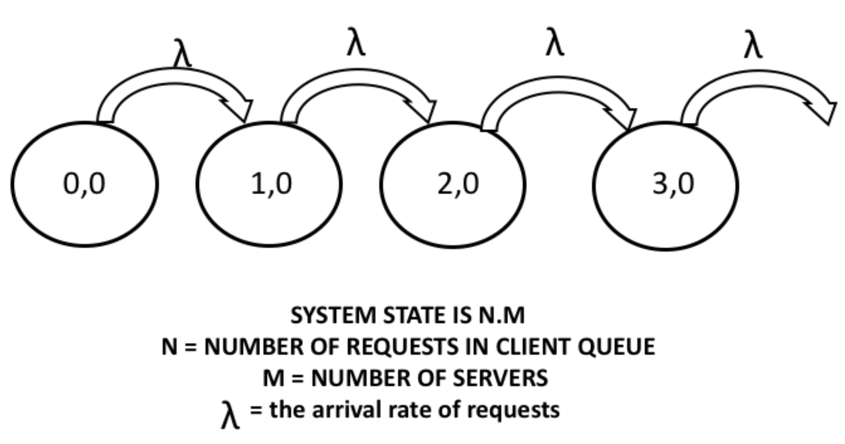
Figure 4.
Markov Model for Non-exhaustive Service.
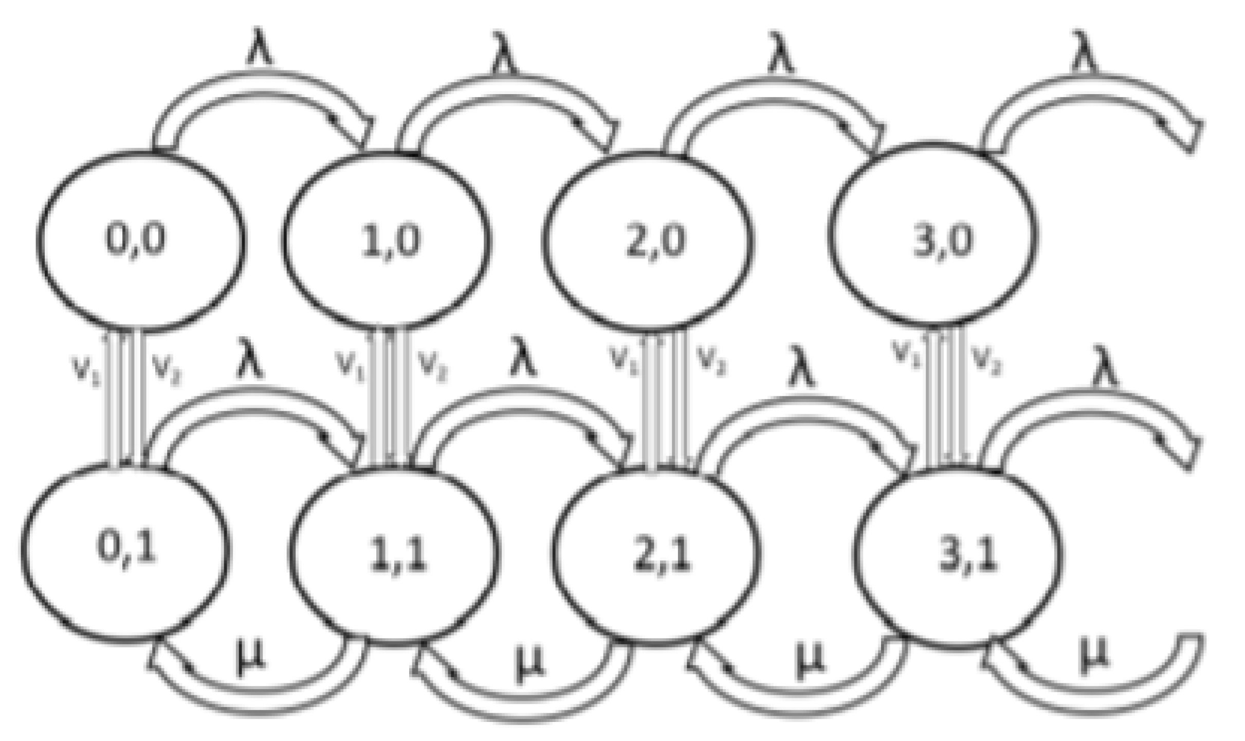
Figure 5.
Graph of One Junction.
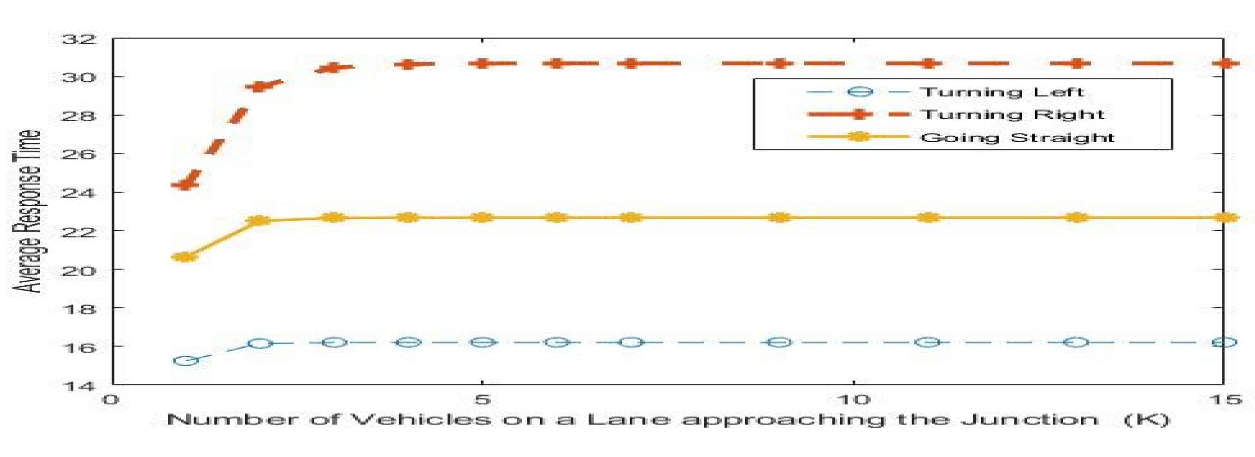
Figure 6.
Graph of Multiple Junction Analysis.
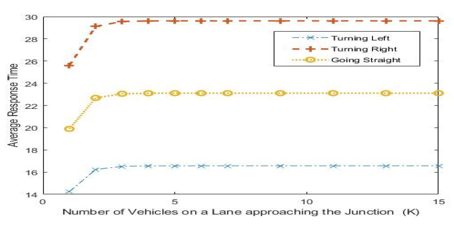
Figure 7.
Markov Chain Model.
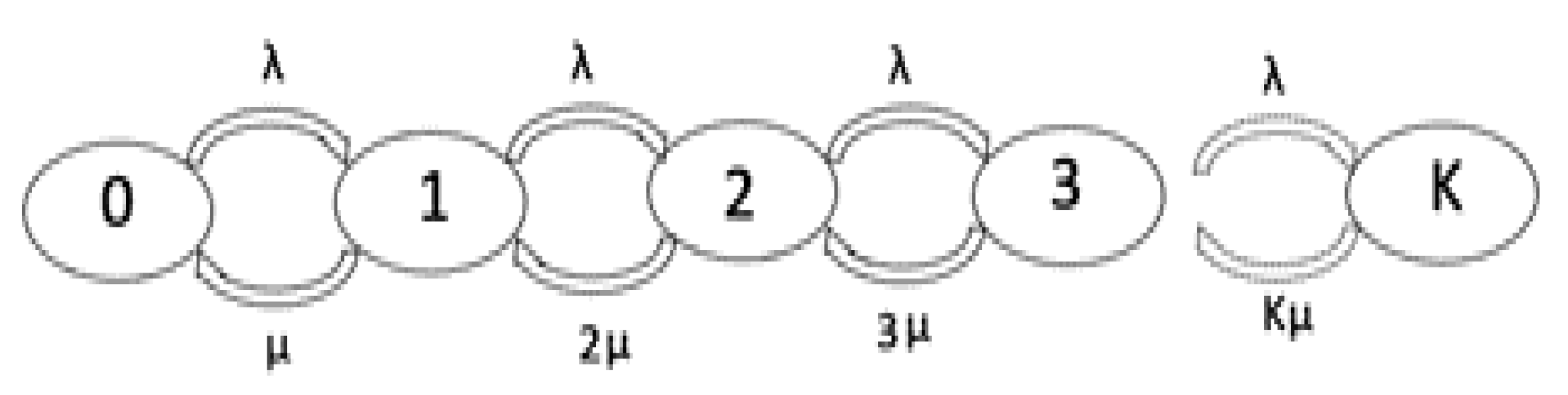
Figure 8.
Link of a Junction.
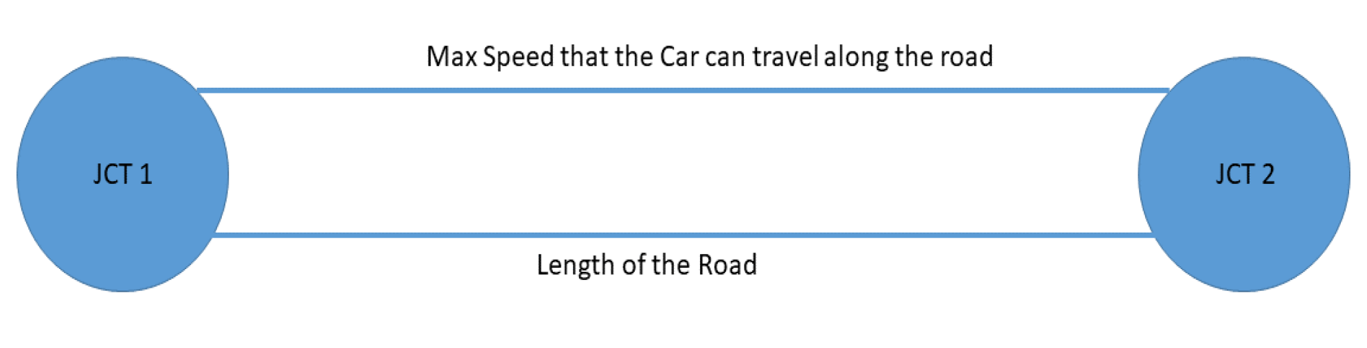
Figure 9.
Three Junction Scenario in Leicester, UK.
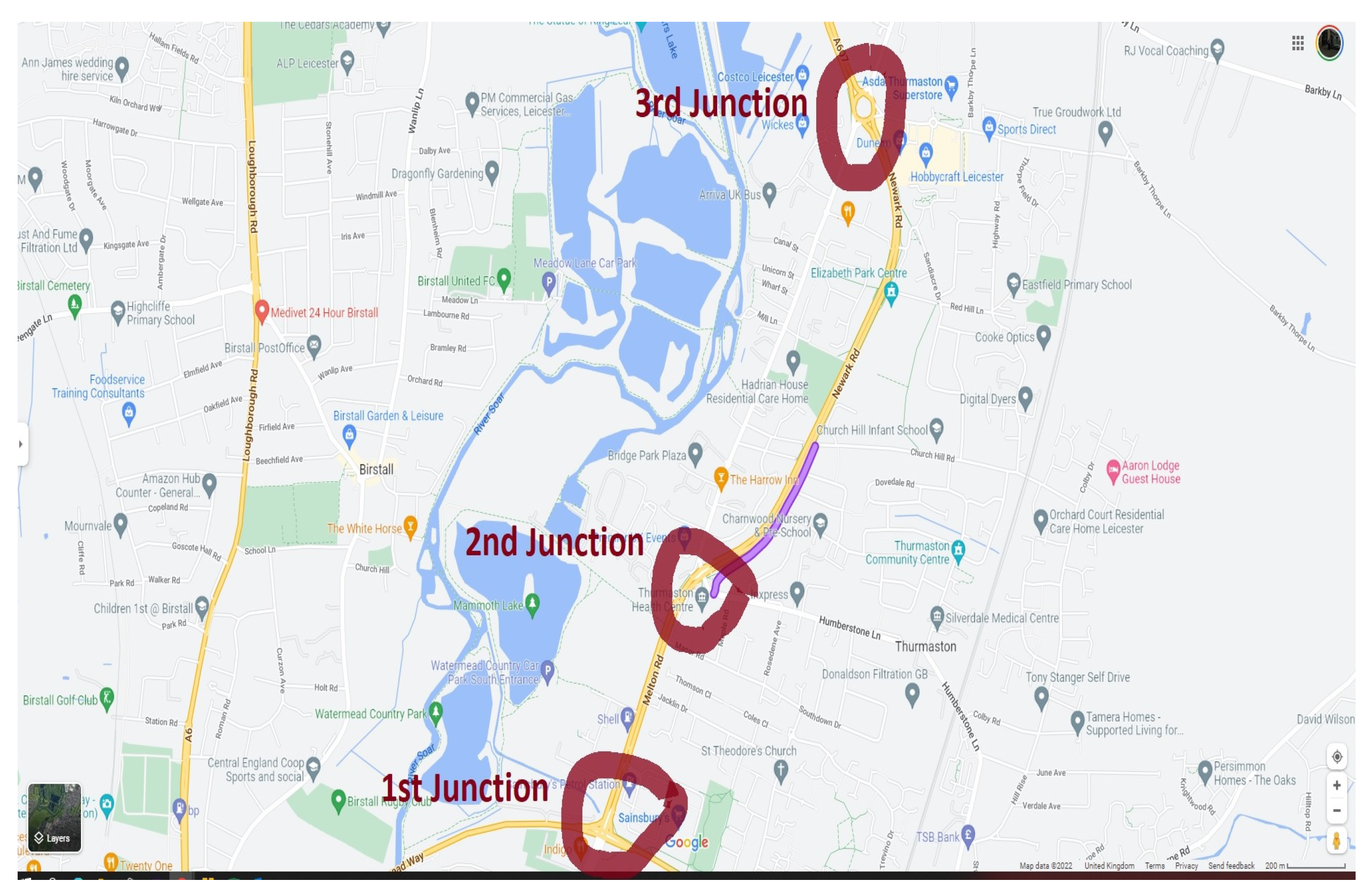
Figure 10.
Three Junction Scenario.
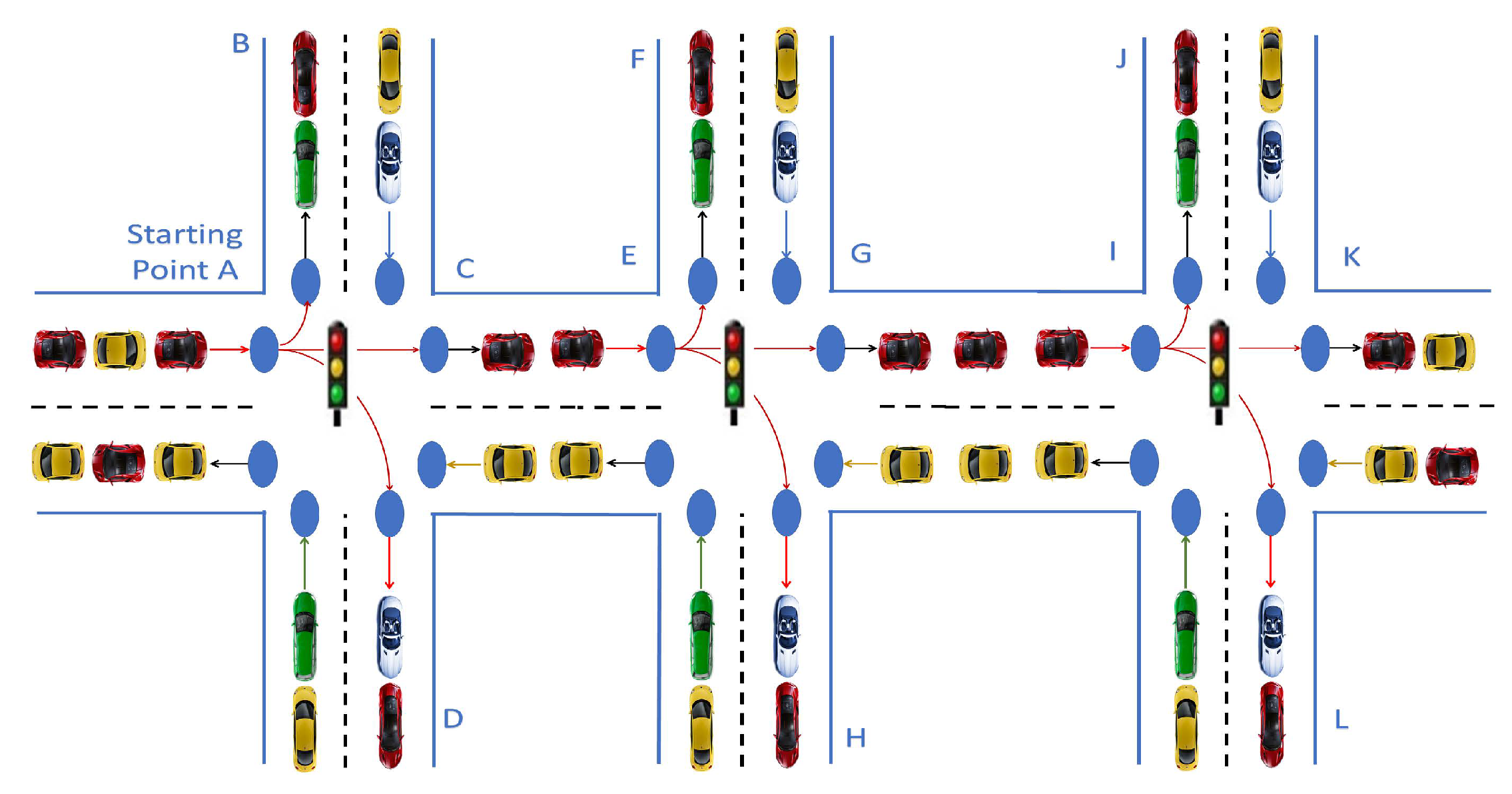
Figure 11.
Three Junctions with Two Links Scenario.
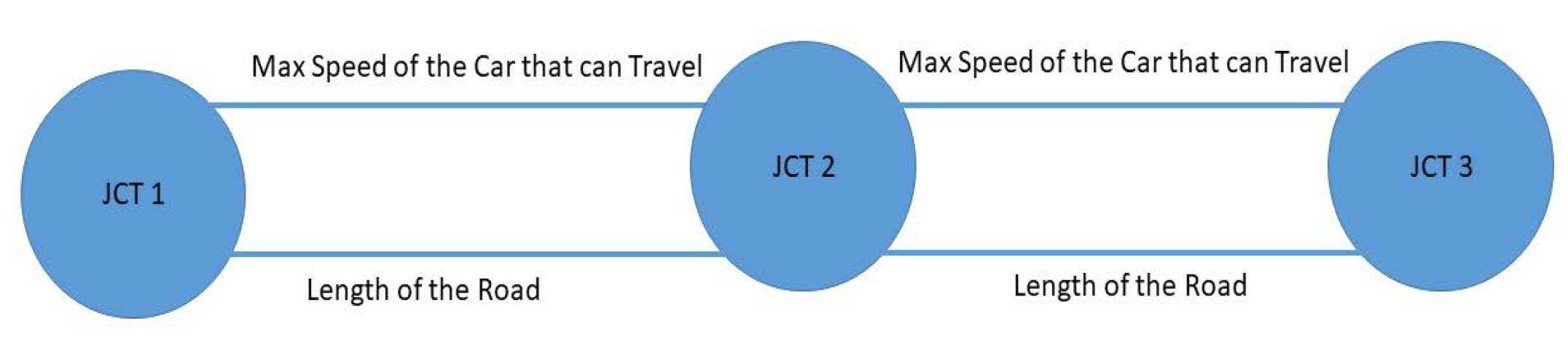
Figure 12.
Three Junctions without Link.
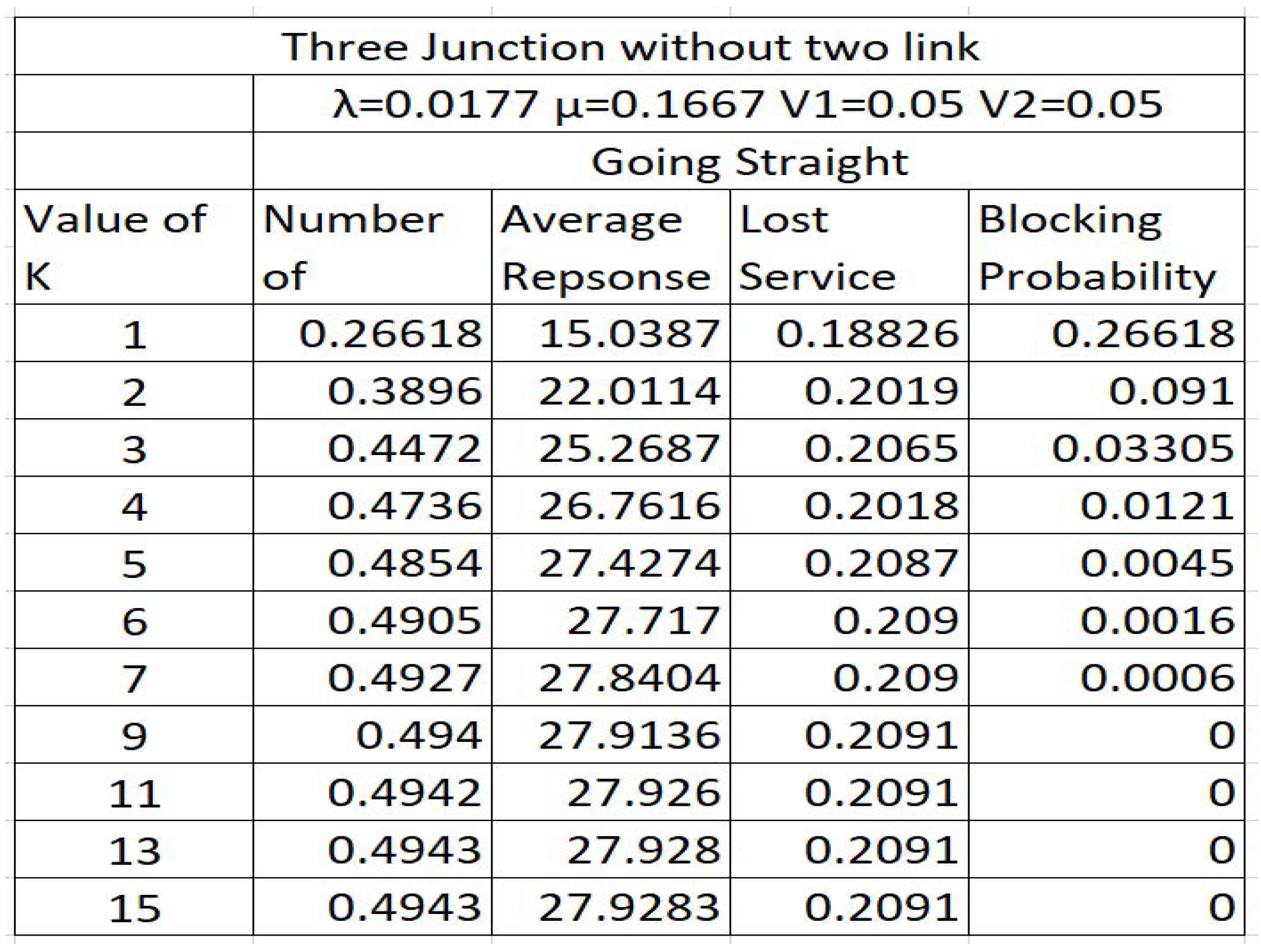
Figure 13.
Three Junctions with Link.
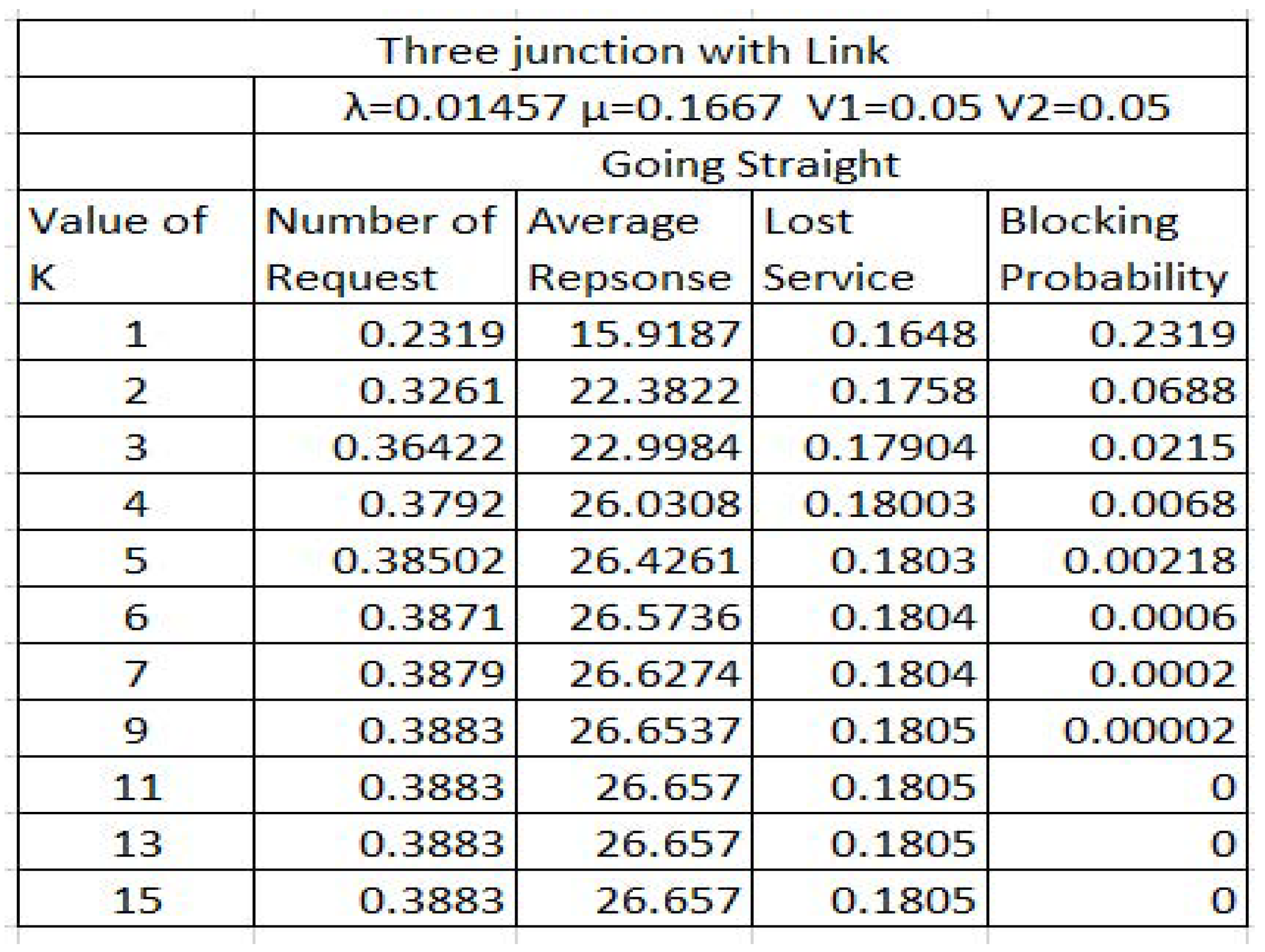
Figure 14.
Sumo Result of Three Junction.
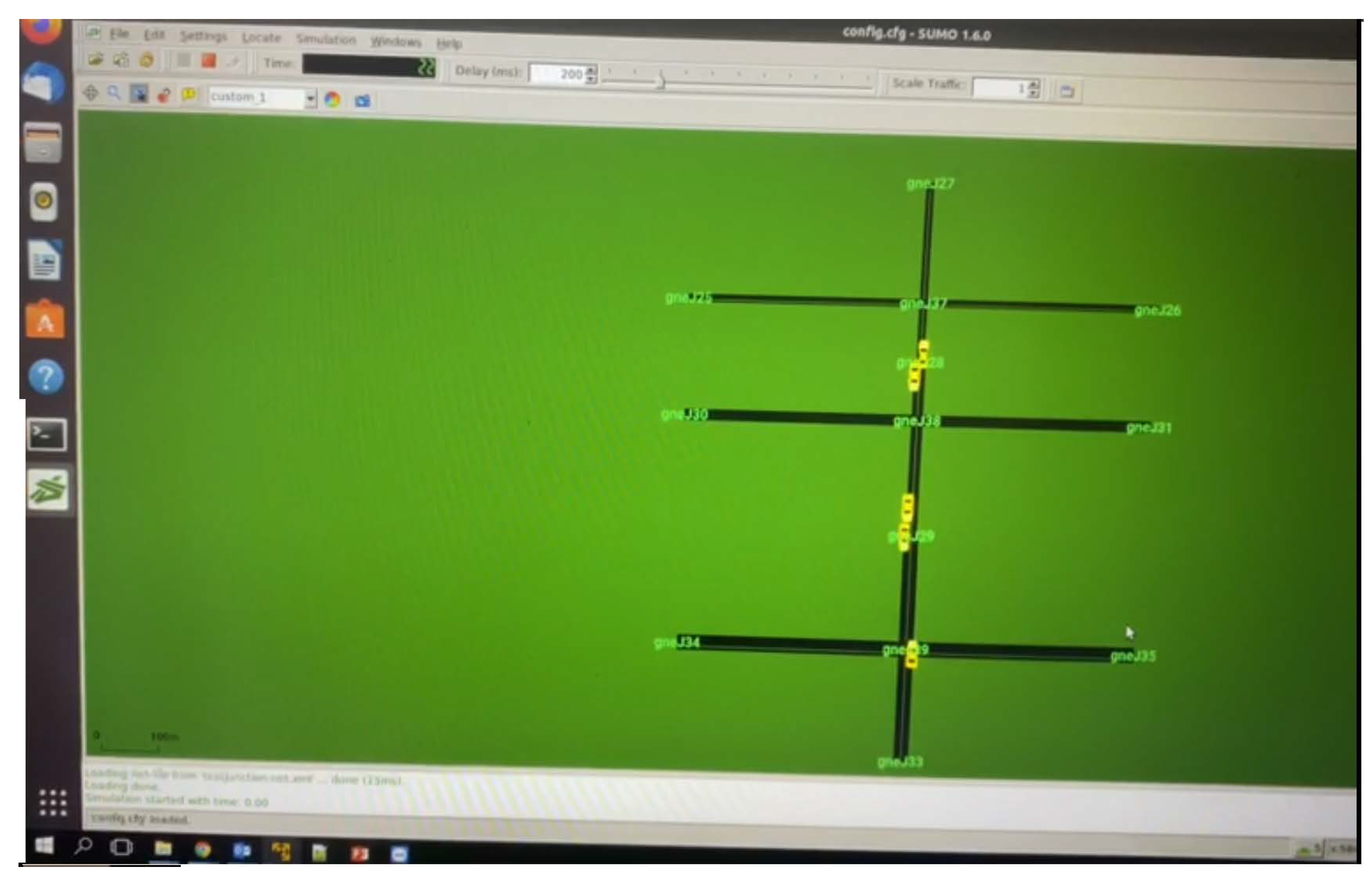
Figure 15.
Shortest Route Calculation.
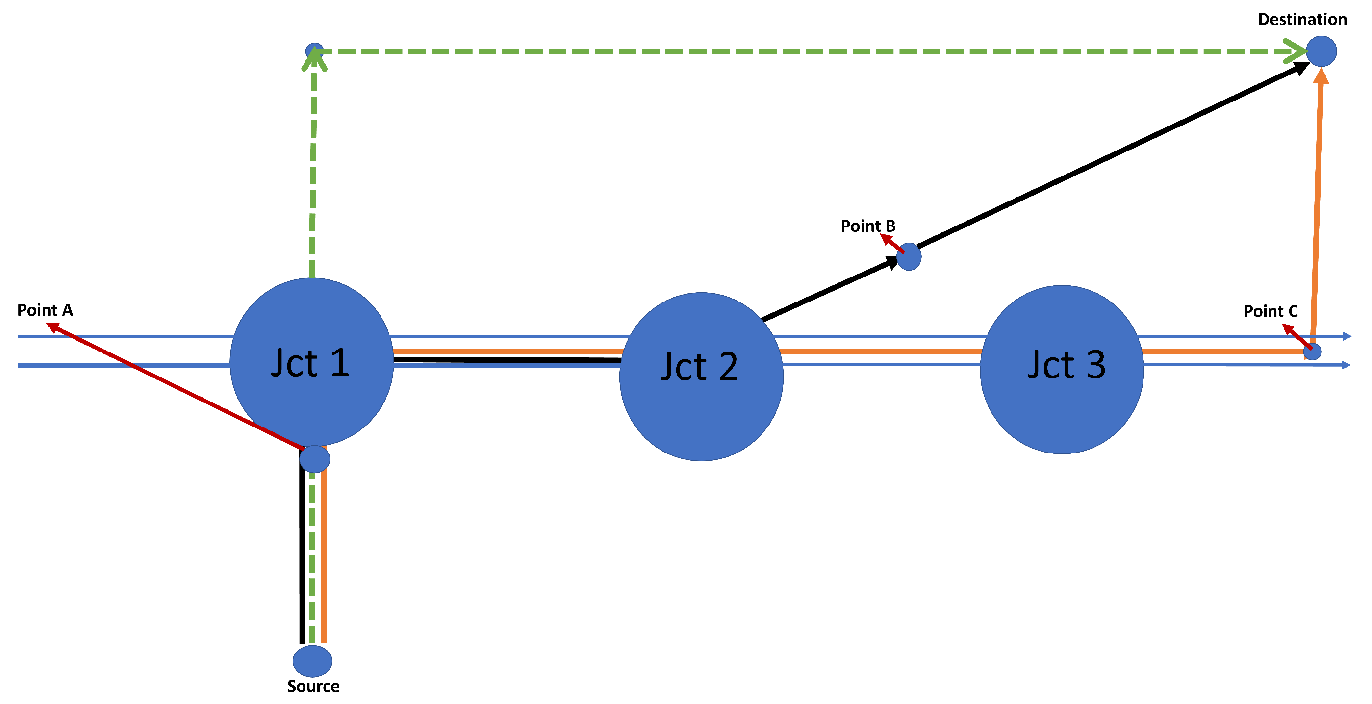

Table 1.
Understanding the Symbols for the Analysis.
| Symbol | Description | Meaning |
|---|---|---|
| Arrival rate of requests | The rate at which requests are made | |
| Service Rate | The rate at which requests are served | |
| State probability in Chain 0 | System in ZSMC | |
| State probability in Chain 1 | System in SBMC | |
| Transition rate from Chain 1 to Chain 0 | Moving from SBMC to ZSMC | |
| Transition rate from Chain 0 to Chain 1 | Moving from ZSMC to SBMC |
Table 2.
Final Travel Time for the Different Routes.
| Route | Travel Time (seconds) |
|---|---|
| Route 1 | 783.3076 |
| Route 2 | 758.0871 |
| Route 3 | 769.5277 |
Disclaimer/Publisher’s Note: The statements, opinions and data contained in all publications are solely those of the individual author(s) and contributor(s) and not of MDPI and/or the editor(s). MDPI and/or the editor(s) disclaim responsibility for any injury to people or property resulting from any ideas, methods, instructions or products referred to in the content. |
© 2024 by the authors. Licensee MDPI, Basel, Switzerland. This article is an open access article distributed under the terms and conditions of the Creative Commons Attribution (CC BY) license (http://creativecommons.org/licenses/by/4.0/).
Copyright: This open access article is published under a Creative Commons CC BY 4.0 license, which permit the free download, distribution, and reuse, provided that the author and preprint are cited in any reuse.


