
Submitted:
14 December 2024
Posted:
16 December 2024
You are already at the latest version
Abstract
We present a slightly more broader framework of variational calculus to accommodate differential equations that are not variational as they stand. We discuss two approaches: The first one utilizes antiexact differential forms as obstruction to variationality, make them vanish that gives constraints for all possible variations. The spproach we discuss describe s of differential equations introducing new functions that make equations variational and then reduce them using a functional constraints. The latter approach incorporates via a not completely standard scheme the classical Dirac reduction approach.
Keywords:
calculus of variations
; variationality
; homotopy operator
; Dirac reduction
; Lagrangian representation
; Dirac constraints
; Poisson operator
; symplectic structure
MSC: 49-02; 49N99
1. Introduction
Calculus of variations is currently a well-established vast discipline with methods ranging from functional analysis [13,17,44] through geometric formulation in jet spaces in terms of variational bicomplex [6,7,8,20,21,22,23,24,30,39,40,42,43,45,46,7].
One of the main problems in the calculus of variations is the Inverse Problem (IP). In basic formulation: given a system of differential equations, check if they are variational, i.e., if they are Euler-Lagrange equations. In this formulation, the solution of the problem is affirmative usually by modification of original problem, e.g., by adding new equations that correct non-variationality of original equations. One way is to use Hamiltonian structures, see e.g., [36] for further references. In a more restricted problem it reads as follows: given the differential equations ’as they stand’ (without any alteration), check if they are the Euler-Lagrange equations for some Lagrangian. The solution to this classical problem dates back to the works of Helmholtz [18], where the well-known Helmholtz conditions were formulated. A recent summary is presented in [20,29,40,47], the formulation in terms of exterior differential systems in [9,32,33], the summary from the viewpoint of classical mechanics is presented in [38], and the perspective from the functional-analytic viewpoint is given in the classical book by Vainberg [44].
In general we will focus on differential expressions over a domain understood as a system of differential equations on a mapping u. It can be composed into functional one-form as
where is an a priori chosen operator, mixing the orders of separate equations. The usual way one defines vertical exterior derivative and a related functional form
where, by definition, where is the total differential operator. Naturally, two functional forms (2) are assumed to be equivalent modulo a divergence term
One can define complementary vertical homotopy operator , defined [25,26,30,44] as
where , and is the linear homotopy between and the center of this homotopy. We assume that of the jet-manifold is connected and star-shaped. This homotopy operator proves to be nilpotent , moreover, there is a homotopy invariance formula
where is an injection to a specific solution .
Similar to [11,12,25,26] one can make use of the homotopy operator (3) to define the set of so called "antiexact" forms
likewise exact forms Suitably, the space of vertical forms can be decomposed into the direct sum as . In addition, one can define projector operators [11,12,25,26],
for which on
Proceeding to a variational representation of a priori given set of equations over a domain one can redefine its lack of variationality in terms of the related non-zero antiexact part: namely, the associated functional one-form (1) can not be represented as a vertical differential for some Lagrangian if the related antiexact part is nontrivial, that is
The paper is organized as follows: in the next section we present a hybrid varaitional problem that is based on antiexact forms, then next section provides some another ways to treating the inverse variational problem by means of introducing some auxiliary a priori Lagrangian one-forms reduced on suitably constructed submanifolds via the corresponding Dirac type constraints.
2. General Approach to a Hybrid Variation Problem
In general, an arbitrary smooth differential system can be rewritten as a functional 1-form
which is naturally decomposable into the direct sum components as
within which the density
is called a quasi-Lagrangian. The splitting (9) can be rewritten as
where, by definition, We can then interpret the identity (11) in the following way: the differential system under regard can be considered as a solution for the following ’optimization’ problem:
for vector fields As the condition (12), in general, is not solvable for all vector fields it is natural to reduce the whole system on the functional submanifold
The obtained this way differential system
becomes a priori Lagrangian on the functional submanifold as
where the Lagrangian is well defined on The latter partially solves the inverse problem of variational representation for the one-form suitably reduced on the functional submanifold . A slight modification of this scheme, based on the hybrid variational analysis, is worked out below.
2.1. The Reduction Scheme and a Related Hybrid Variational Problem
Let us consider a smooth differential system on the jet -manifold and analyze its virtually assumed Lagrangian structure, that is the existence of such a smooth mapping that this differential system is equivalent to the gradient grad which can be written down in the simplest case as
where one assumes that and , , is some nondegenerate operator endomorphism of the cotangent space . In the general case it is also well known that the problem under regard is not practically resolvable, if the differential system grad for some nonlinear and nondegenerate mapping . Yet, if we are interested in representing a given differential system within some kind of a hybrid variational formalism, one can try to express the relationship (16) in the differential geometric language on the jet-manifold as a differential form
where a mapping at denotes the usual [1,11,12,25,26,44] Poincare homotopy operator and is the natural bi-linear form on The representation (17) makes it possible to write down the following hybrid variational problem
on a functional submanifold defined via the functional relationship
The latter easily gives rise to the gradient relationship
for the Lagrangian and all completely equivalent to that of (17), reduced on the submanifold Thus, one can formulate the following proposition.
Proposition 1.
Any smooth differential system on the jet -manifold admits the hybrid variational representation
on the functional submanifold ,defined by the relationship(19).
As a simple example one can consider the Burgers type dissipative evolution equation
on the jet-manifold for a function where a parametric function satisfies the adjoint evolution equation
on the related jet-manifold Having taken the nondegenerate operator endomorphism where we can easily check that the submanifold is defiend by the differential form vanishing identically. The latter makes it possible to state that the corresponding hybrid variational interpretation (21) becomes a true variational problem for the combined Burgers type system (22) and (23).
2.2. An optimal control problem aspect and the related Dirac type reduction scheme
As a typical example, let us consider a dynamical system
on a toric functional manifold which a priori is not of variational type, make its smooth functional parametrical extension
with respect to a toric functional variable for some smooth differential functional relationship on the product and pose the following Bellman-Pontriagin type optimal control problem [3,31] subject to some smooth Lagrangian density on a temporal interval
for a fixed under the condition that the evolution flow (25) possesses a smooth conserved quantity that is on the combined manifold for all The latter, in particular, means that we need to determine such an additional evolution flow
on the extended control manifold which will ensure the existence of the mentioned above smooth conserved quantity The problem above is solved [31] by means of construction of the extended Lagrangian functional
supplemented with Lagrangian multipliers and almost everywhere with respect to the temporal parameter and next determining its critical points:
for all jointly with the condition for The obtained functional relationship (29) under the condition reduces to the following generalized Noether-Lax condition
on the Lagrangian multiplier as the following Noether-Lax equality
holds a priori for any smooth conservation law of the joint dynamical system
on the combined manifold
A solution to the condition (30) allows the unique representation as the direct sum of its skew symmetric and strictly symmetric components, satisfying, respectively, the following differential-functional equations:
where, by definition, on and
where, by definition, on for all Under the a priori assumed condition that the evolution flow (32) is a Hamiltonian system on the functional manifold with respect to the related symplectic structure mapping the differential-functional equation (33) is always [1,2,4] solvable, giving rise to the known differential-geometric relationship
subject to which the following compatible vector field representation
holds on Simultaneously, the differential-functional equation (34) is also always [1,2,4] solvable under the condition that for some conserved quantity of the evolution flow (25) regardless of whether the evolution flow (25) on is Hamiltonian or not. The latter means, evidently, that it is also of variational type, which can be suitably reduced via the Dirac scheme on the functional submanifold
concerving its variational type on following from the stated above Hamiltonian representation (36).
2.3. Example: Burgers Equation
Concerning the diffusion type Burgers equation example, considered before,
on the functional manifold , treated within the optimal control problem scheme above, there is suggested the following way of embedding the flow (38) into the Dirac type constrained variariational picture:
- as a result, owing to the fact that the reduced on the submanifold dynamical system (38) persists to be Hamiltonian too, it will represent a true Burgers dynamical system as the one a priori representable in the variational Lagrangian form on this submanifold.
Subject to this Burgers dynamical system (38) the analytic scheme above gives rise to the following evolution flow
on the parametric functional manifold which jointly with the flow (38) represents the following Hamiltonian system:
where is the corresponding canonical symplectic structure mapping on :
and is the related to it conserved Hamiltonian function:
Having now applied the classical Dirac type reduction scheme to the Hamiltonian system (43) upon the submanifold one obtains a true Burgers dynamical system (38) as a Hamiltonian system on this submanifold a priori possessing, respectively, the related variational Lagrangian representation. To demonstrate this property, we will make use of the fact that the obtained Hamiltonian system possesses [4,5,34,35] a countable hierarchy of functionally independent conserved quantities amongst them the Hamiltonian (45), whose functional gradients are calculated analytically via the recursion scheme:
where the gradient recursion operator is given by the following integro-differential operator expression:
Having calculated the conserved gradient expression ∈
and taken into account that it is invariant with respect to the vector field (43) and ensuing from the linear Noether-Lax relationship
one can proceed to the invariant reduction of the Burgers evolution flow (38) upon the functional submanifold Preliminarily, we need to take the invariant Lagrangian function density and reduce our Hamiltonian flow (43) on the 6-dimensional invariant submanifold
as a flow on taking into account [4,14,15,16] the classical Gelfand-Dickey relationship:
determining on the submanifold the nondegenerate symplectic structure From (50) one easily ensues that the Hamiltonian flow (43) on the submanifold being Hamiltonian with respect to the constructed above symplectic structure can be reduced via the Dirac scheme upon the submanifold
thus reducing it to the initial Burgers flow (42), equivalently representing it as a Lagrangian variational problem on the jet-submanifold
3. Schwinger’s Variational Principle as a Constrained Problem
In this section we study Schiwnger’s ’third way’ of formulating variational problem [10,28,41]. In this approach we make independent variations of field, its tangent and cotangent components. At first it seems that one requires space for this variation, however, one use only and a constraint.
Consider a functional manifold M and a Lagrangian
representable as smooth mapping in local coordinates Its Schwinger extension is defined as a mapping where is some analytical expression, whose simplest form looks as
where variables and are assumed to be independent. Then the following proposition holds.
Proposition 2.
Proof.
In replace by an arbitrary element , and introduce a vector of Lagrange multipliers for the constraint This gives (53).
From the variation with respect to v and the multipliers p independently we obtain
This gives Euler-Lagrange equations for the density and the definition of momentum . □
One can see that by construction, is the canonical momentum playing the role of a Lagrange multiplier subject to the tangent element Since the Hamiltonian function is defined as modulo the determining relationship
one gets right away the classical Hamiltonian equations
Turn back now to our problem of Lagrangian representation of a given evolution equation
on a jet-manifold whose Lagrangian form is either not known or not existing on the whole. To suggest a partial solution to this problem, one can consider a close enough to (55) Lagrangian evolution equation
on a jet-manifold whose invariant reduction on the functional submanifold
defined by the evolution invariant constraints will coincide with the given evolution equation (55). This means that there exists some smooth extended Schwinger type functional
on the whole manifold for which the least action condition
with respect to variables and the corresponding Lagrangian multipliers reduces on the submanifold to the given evolution equation (55). This means that on the submanifold
The latter makes it possible to deduce from (59) the multiplier
and, suitably, the next multiplier Thus, one can formulate the following proposition.
4. Conclusions
We proposed some ways of formulation of the variational problem for problems that are not variational. One uses antiexact forms to construct a constraints for space of all possible variations. The other approach extends the number of variables and equations to make the new system variational and then reduce the extended jet space to submanifold that vanish these additional variables. Still, the algorithmic way of such extension is to be found.
Acknowledgments
The research of R.K. was supported by the GACR grant GA22-00091S, the grant 8J20DE004 of the Ministry of Education, Youth and Sports of the CR, and the Masaryk University grant MUNI/A/1092/2021. A.P. is grateful to the Department of Mathematical Sciences for invitation to visit the UAE University within the UAEU grants G00003658 and G00004159.
Appendix A. Dirac Constraints
To unify all notions related to Dirac’s theory of constraints, we give a short summary. We will base on a few resources [1,19,27,37].
We consider a finite-dimensional symplectic manifold with respect to the symplectic form endowed with a set of smooth functional constraints These constraints naturally determine the smooth submanifold under condition of independence of these constraints, i.e.,
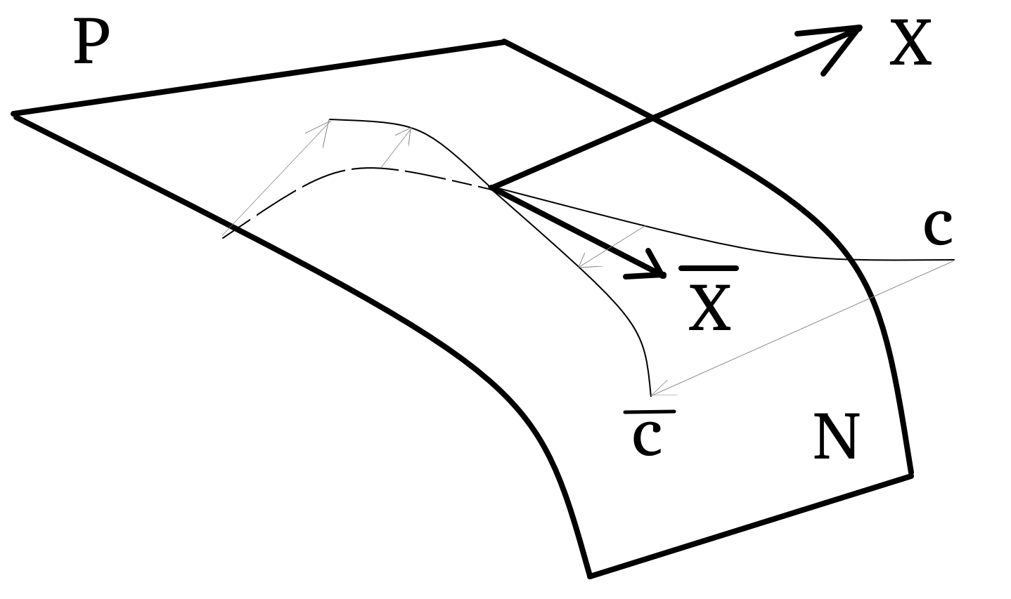
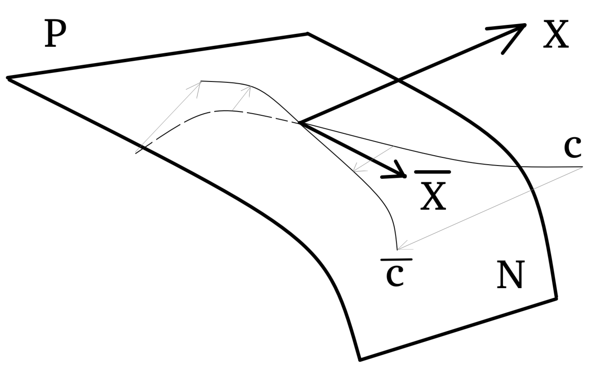
Any vector field defined by a smooth mapping via the relationship and called Hamiltonian, can be projected to the vector on the invariant submanifold defined by the projected Hamiltonian by In particular, this mapping projects any trajectory onto as presented in Fig. Figure A1.
Figure A1.
The projection of X from the symplectic space P onto a submanifold N. Then the trajectory c is also projected onto the trajectory in N.
Figure A1.
The projection of X from the symplectic space P onto a submanifold N. Then the trajectory c is also projected onto the trajectory in N.
The first step is to find the projection on the submanifold defined by the conditions Thus, one can write down the decomposition
where are so called Lagrange multipliers and are the related symplectic skew-gradient vector fields, connected with the symplectic structure via the relationship for Choosing now as generated by a smooth function and taking into account the definition of its Poisson bracket with an arbitrary smooth function we easily obtain that
for every If the matrix is nondegenerate on the submanifold it allows to determine the vector of the Lagrange multipliers as
where is the related vector of the so called second order constraints functions. Having substituted the result (A3) into the decomposition (A1) and taken its convolution with any differential one derives finally the classical Dirac bracket expression
on the submanifold for arbitrary smooth functions reduced on the submanifold
If we are interested in studying the evolution of a specially chosen vector field reduced on the invariant submanifold the condition should be a priorisatsified. If it is not a case, that is yet already and where there should be considered the Hamiltonian flow subject to the Poisson bracket (A4)
reduced already on the submanifold If additional constraints satisfy the conditions for some constant matrix they are called the first class constraintsand should not be taken into account for constructing the reduced Dirac bracket (A4). The first class constraints are responsible for so called gauge transformations. Adding the secondary constraints and reiterating the algorithm, the latter stops at some point. These and other related questions are discussed in detail in physics-oriented books [19,37].
References
- R. Abraham, J. Marsden, Foundations of Mechanics, Second Edition, Benjamin Cummings, NY, 1984.
- V.I. Arnold, Mathematical Methods of Classical Mechanics, Springer, NY, 1989.
- R.E. Bellman, Dynamic Programming, Dover, 2003.
- D. Blackmore, A.K. Prykarpatsky and V.H. Samoylenko,Nonlinear Dynamical Systems of Mathematical Physics, World Scientific, NJ, 2011.
- Prykarpatsky, Y.A.; Urbaniak, I.; Kycia, R.A.; Prykarpatski, A.K. Dark Type Dynamical Systems: The Integrability Algorithm and Applications, Algorithms 2022, 15, 266. [CrossRef]
- R. Aldrovandi, R.A. Kraenkel, On exterior variational calculus, J. Phys. A: Math. Gen. 21 1329 (1988). [CrossRef]
- R. Aldrovandi, J.G. Pereira, An Introduction to Geometrical Physics, 2nd edition, World Scientific 2016; Chapter 20.
- I.M Anderson, Variational Bicomplex, unpublished script.
- I. Anderson, G. Thompson, The inverse problem of the calculus of variations for ordinary differential equations, 98, 473, Memoirs of the American Mathematical Society, 1992.
- W. Dittrich, The Development of the Action Principle: A Didactic History from Euler-Lagrange to Schwinger, Springer, 2021.
- D.G.B. Edelen, Applied Exterior Calculus, Dover Publications, Revised edition, 2011.
- D.G.B. Edelen, Isovector Methods for Equations of Balance, Springer, 1980.
- I.M. Gelfand, S.V. Fomin, Calculus of Variations, Dover Publications, 2000.
- I.M. Gelfand, L.A. Dickey, Integrable nonlinear equations and Liouville’s theorem, Funct. Anal. Appl. 13 (1979), 8–20.
- L.A. Dickey, Integrable nonlinear equations and Liouville’s theorem, I. Communications in Mathematical Physics, Commun. Math. Phys. 83 (1981), 345–360.
- L.A. Dickey, Integrable nonlinear equations and Liouville’s theorem, II, Communications in Mathematical Physics, 82 (1981), 361–375.
- M. Giaquinta, S. Hildebrandt, Calculus of Variations, 2 vols. Springer 2010.
- H. Helmholtz, Ueber die physikalische Bedeutung des Prinicips der kleinsten Wirkung, J. Reine Angew. Math. 137 (1887).
- M. Henneaux, C. Teitelboim, Quantization of Gauge Systems, Princeton University Press, 1994.
- I. Khavkine, Presymplectic current and the inverse problem of the calculus of variations, J. Math. Phys. 54, 111502 (2013). [CrossRef]
- D. Krupka, Introduction to Global Variational Geometry, Atlantis Press, 2015.
- D. Krupka, Global variational theory in fibred spaces, in Handbook of Global Analysis, Elsevier 2007.
- O. Krupková, G.E. O. Krupková, G.E. Prince, Second Order Ordinary Differential Equations in Jet Bundles and the Inverse Problem of the Calculus of Variations, in Handbook of Global Analysis, Elsevier 2007.
- O. Krupkova, The Geometry of Ordinary Variational Equations, Springer 1997.
- R.A. Kycia, The Poincare Lemma, Antiexact Forms, and Fermionic Quantum Harmonic Oscillator, Results Math 75, 122 (2020). [CrossRef]
- R.A. Kycia, The Poincare lemma for codifferential, anticoexact forms, and applications to physics, Results Math 77, 182 (2022). [CrossRef]
- J.E. Marsden, T.S. Ratiu, Introduction to Mechanics and Symmetry: A Basic Exposition of Classical Mechanical Systems, Springer, 2nd edition 2023.
- K. A. Milton, Schwinger’s Quantum Action Principle: From Dirac’s Formulation Through Feynman’s Path Integrals, the Schwinger-Keldysh Method, Quantum Field Theory, to Source Theory, Springer, 2015.
- Z. Muzsnay, G. Thompson, Inverse problem of the calculus of variations on Lie groups, Differential Geometry and its Applications, 23, 3, 257–281 (2005). [CrossRef]
- P.J. Olver, Applications of Lie Groups to Differential Equations, 2nd edition, Springer, 2000.
- L.S. Pontryagin,V.G. Boltyanski, R.S. Gamkrelidze and E.F. Mishchenko, The Mathematical Theory of Optimal Processes, Interscience, 1962.
- T. Doa, G. Prince, New progress in the inverse problem in the calculus of variations, Differential Geometry and its Applications, 45, 148–179 (2016). [CrossRef]
- G.E. Prince, D.M. King, The inverse problem in the calculus of variations: nonexistence of Lagrangians, F. Cantrijn, B. Langerock (Eds.), Differential Geometric Methods on Mechanics and Field Theory: Volume in Honour of Willy Sarlet, Academia Press, Gent, 131–140 (2007).
- A.K. Prykarpatski, P.Y. Pukach, M.I. Vovk, Symplectic Geometry Aspects of the Parametrically-Dependent Kardar–Parisi–Zhang Equation of Spin Glasses Theory, Its Integrability and Related Thermodynamic Stability. Entropy 2023, 25, 308. [CrossRef]
- A.K. Prykarpatski, V.A. Bovdi, On the Lie-Algebraic Integrability of the Calogero-Degasperis Dynamical System and Its Generalizations, Contemporary Mathematics, Contemporary Mathematics, 4(4) 2023, 750-768; http://ojs.wiserpub.com/index.php/CM/.
- A.K. Prykarpatsky , I.V. Mykytiuk, Algebraic Integrability of Nonlinear Dynamical Systems on Manifolds, Springer 1998.
- H.J. Rothe, K.D. Rothe, Classical and Quantum Dynamics of Constrained Hamiltonian Systems, World Scientific Publishing Company 2010.
- R. M. Santilli, Foundations of Theoretical Mechanics I, Springer-Verlag Berlin Heidelberg 1978.
- D. J. Saunders, The Geometry of Jet Bundles, Cambridge 1989.
- D.J. Saunders, Thirty years of the inverse problem in the calculus of variations, Reports on Mathematical Physics, 66 1 43–53 (2010). [CrossRef]
- J. Schwinger at al., Classical Electrodynamics, Westview Press, 1998.
- T. Tsujishita, On variation bicomplexes associated to differential equations, Osaka J. Math. 19 (1982), 311-363.
- W.M. Tulczyjew, The Euler-Lagrange resolution, in Lecture Notes in Mathematics 836 -48, Springer-Verlag, 1980.
- M.M. Vainberg, Variational Methods for the Study of Nonlinear Operators, Holden-Day 1964.
- A. Vinogradov, A spectral sequence associated with a non-linear differential equation, and the algebro-geometric foundations of Lagrangian field theory with constraints, Sov. Math. Dokl. 19 (1978) 144-148.
- R. Vitolo, Variational sequences, in Handbook of Global Analysis, Elsevier 2007.
- D. Zenkov, The Inverse Problem of the Calculus of Variations, Atlantis Press, 2015.
Disclaimer/Publisher’s Note: The statements, opinions and data contained in all publications are solely those of the individual author(s) and contributor(s) and not of MDPI and/or the editor(s). MDPI and/or the editor(s) disclaim responsibility for any injury to people or property resulting from any ideas, methods, instructions or products referred to in the content. |
© 1996 by the authors. Licensee MDPI, Basel, Switzerland. This article is an open access article distributed under the terms and conditions of the Creative Commons Attribution (CC BY) license (https://creativecommons.org/licenses/by/4.0/).
Copyright: This open access article is published under a Creative Commons CC BY 4.0 license, which permit the free download, distribution, and reuse, provided that the author and preprint are cited in any reuse.


