Submitted:
09 December 2024
Posted:
10 December 2024
You are already at the latest version
Abstract
This study investigates the relationship among lane width, velocity, and accident rates to enhance understanding their impact on road safety and transportation. Analysis of data from 320 urban arterial sections in Utah indicated that narrower lane widths can improve road safety. Reduced vehicle speeds were related to narrower lanes on urban arterials, which did not result in increased collision rates. Reducing one foot in lane width led to an average speed decrease exceeding one mph. Additional factors influencing speed on urban arterials encompass the number of lanes, the existence of medians, on-street parking, roadside obstructions, and block length. Safety modeling indicated no clear correlation between lane width and total crash frequency per mile. Injury crash rates positively correlated with lane width and speed, suggesting that broader lanes and elevated speeds augment the probability of injury crashes. Additional critical elements affecting crash statistics comprised the number of lanes and the Average Annual Daily Traffic (AADT) per lane (in thousands). The study endorses the reduction of lane widths as a viable approach to augment road safety and boost urban transportation infrastructure. The results provide essential direction for policymakers and transportation authorities aiming to enhance road safety and efficiency.
Keywords:
lane width
; speed
; crash likelihood
; cross-sectional road design
; urban arterial
; safety modeling
1. Introduction
Reducing vehicle lane widths is an effective method for decreasing vehicle speeds and enhancing road safety. The street design guidelines, formulated by the American Society of Civil Engineers (ASCE), the Institute of Transportation Engineers (ITE), the National Association of Home Builders (NAHB), and the Urban Land Institute (ULI), advocate for the selection of minimum lane widths that fulfill fundamental requirements without superfluity. This method reduces construction as well as maintenance expenses while producing a more sustainable and livable society. Additionally, narrower lanes can create space for infrastructure that facilitates active mobility.
The effect of narrower travel lanes on safety remains contentious, as research presents inconclusive results about the consistent enhancement of road safety through lower lane widths. An initial study by Swift et al. (1997) indicated that narrower lanes on residential streets were associated with reduced injury-related accidents [1]. Recent studies suggest that the safety implications of smaller lanes can differ based on traffic volume and roadway type. Narrow lanes have been shown to enhance safety on rural roads, but on highways and urban arterial roads, they are frequently associated with an increased risk of collisions [2,3,4,5]. The correlation between lane width and driving speeds is intricate and not entirely comprehended. Narrower lanes typically correlate with decreased speeds, enhancing traffic safety; however, other elements like road markings and medians also affect drivers' perceptions of lane width and speed, particularly on curved sections compared to straight highways [6]. This underscores the necessity of meticulously considering multiple factors—such as traffic volume, capacity, level of service, speed, cross-sectional alignment, development type, and other geometric characteristics—when examining the relationship between lane width and vehicle speeds [7].
The paper comprehensively investigates the relationships among lane width, speed, and crash rates on urban arterial roadways in Utah. This analysis examines the influence of lane width alterations on driving speeds to enhance the understanding of the relationship between lane width and traffic safety. Data on safety metrics (including total and injury crash rates), roadway capacity, pedestrian traffic volume, and agency expenditures (including construction and maintenance costs) are gathered and evaluated to assess current practices and pinpoint possibilities and problems in road width design. Furthermore, implementing narrower roads can enhance community livability by promoting active transportation methods.
2. Literature Review
2.1. Safety
2.1.1. Lane Width
Reducing lane widths on urban arterials can create additional space for pedestrians and bicycles, including wider sidewalks, landscaped buffers, shorter pedestrian crossings, and dedicated bike lanes. It can also facilitate the development of supplementary on-street parking areas. Nevertheless, safety must be considered when determining adequate lane widths for these routes. Prior research has yielded inconclusive findings concerning the correlation between lane width and road safety on urban arterials, suggesting that this relationship may be contingent upon several contributing factors [7,8].
Studies indicate that the impact of lane width on safety outcomes varies across urban and rural environments. Research in rural regions has demonstrated a significant correlation between accident risk and road design features, including lane, shoulder, and median widths [9,10,11]. Nonetheless, other research indicates that lane and shoulder widths exert negligible effects on crash severity, whereas the type of shoulder plays a more crucial role, decreasing crashes by 30–70% [12]. These findings contrast previous studies on two-lane rural roadways, which linked broader shoulders to heightened crash severity [13].
Likewise, studies examining the correlation between lane width and safety in metropolitan environments yield inconclusive findings. A study investigating non-freeway urban roads found an association between broader vehicle lanes, smaller shoulders, and a decreased incidence of roadside and midblock crashes [14]. Conversely, several studies on urban streets demonstrated that smaller lanes reduce accidents [8,15,16]. The contradictory results emphasize the intricacy of assessing the effect of lane width on safety in urban environments.
Manuel et al. (2014) investigated the impact of road width on safety for urban collector highways using negative binomial (NB) safety performance functions (SPFs). Their findings revealed that longer segments, elevated traffic volumes, increased access-point density, and midblock alterations (such as crossroads or driveways) were positively associated with higher collisions. In contrast, roadway width showed a negative and statistically significant correlation with crashes, indicating that narrower roadways may be linked to decreased crash frequency.
Lane width, route curvature, roadside development, and traffic control also affect vehicle speed. A previous study identified two principal methodologies for measuring this relationship: quasi-experimental studies (before and after) of individual roadway segments and comparative studies of various routes with differing lane widths [17]. The research determined that the literature lacks consensus on the correlation between lane width and speed.
In the NCHRP 330 report, Douglas Harwood (1990) analyzed the efficient application of roadway width on urban arterials at 35 locations in five states [18]. He emphasized assessing several options for employing streets with identical curb-to-curb dimensions. Harwood accounted for other variables that could affect efficacy to guarantee precise outcomes, including traffic volume, vehicle composition, capacity (level of service), prevailing speeds, cross-sectional alignment, kind of development, and access to neighboring properties. The research was specifically confined to urban arterials with speed limits of 45 mph or lower, and its findings were predominantly derived from lane width.
- Lane width narrower than 11 feet can be used effectively for urban arterial improvements, while narrower lanes may result in some accident types.
- 10 feet lane width is widely accepted by engineers with reduced or unchanged accident rates.
- Based on its impact on the accident rate, a lane width of less than 10 feet should be used cautiously.
Roadside elements, such as street trees and nearby parking, significantly influence traffic management and give drivers a sense of spatial orientation. The positioning and visibility of roadside objects are crucial for traffic safety. In addition to establishing a safe zone for roadside elements, several geometric designs are linked to road safety [19]. Lane width is a feature that can enhance safety. Hauer's study indicates that wide lanes do not correlate with safety, asserting that the threshold for safer roads is 11 feet [20]. Dumbaugh (2000) found that 11 ft lanes have 11% fewer mid-block collisions than 12.5 ft lanes. This contrast is far more pertinent for harmful and lethal collisions [19]. The driver's assessment of the road environment and response to associated dangers is the most important aspect of enhancing safety. The rationale for increased accidents on broader highways is as follows.
"Features like wider lanes and clear zones seem to diminish the driver's perception of risk, providing an inflated yet misleading sense of security, which may lead to behaviors that heighten the probability of a crash."
It has been suggested that roadway design should prioritize "drivers' perception of risk" over rigid compliance with traditional technical requirements. When drivers assess the safe speed as exceeding the posted speed limit, they are more inclined to exceed it. Moreover, integrating practical road design elements and enacting traffic calming strategies can substantially improve safety, promoting driver conduct that more closely aligns with traffic safety goals.
2.1.2. Shoulders
One of the critical variables that influence crashes is the shoulder. Roads with shoulders can indirectly influence crash frequencies by affecting average vehicle speed [21,22,23]. This suggests that the presence of shoulder lanes may increase vehicle speeds, which, in turn, produce higher crash frequencies. Removing or narrowing shoulder lanes is likely a more effective way of managing speeds and, consequently, reducing collisions than narrowing lane widths [23].
Increasing shoulder width is directly associated with higher crash rates [22,24]. For instance, Bamzai et al. (2011) suggested that shoulders narrower than 2.44 meters could potentially reduce shoulder-related crashes [24]. Additionally, Gitelman et al. (2019) discovered that widening unpaved shoulders beyond 0.9 meters increased the risk of crashes, particularly injuries and total crashes, with a 5% increase in crash risk for each additional 0.1-meter extension [25]. However, the lowest crash risks were observed with total shoulder widths of around 3 meters or wider and narrower shoulders of less than 1 meter.
On the other hand, another body of literature found that roads with shoulders are likely to have lower crash frequencies [25,26,27]. For example, Gitelman et al. (2019) found that widening the shoulder to 2.2 meters increased crash risk. However, crash frequency decreased when the shoulder was expanded beyond this point. A driving simulation study also indicated that shoulders could reduce head-on collisions, as drivers tend to steer farther away from oncoming traffic [21].
2.1.3. Number of Lanes
Previous studies have also shown that the number of lanes plays a significant role in road safety [28,29,30]. For instance, Abdel-Aty and Radwan (2000) found that crash rates increased as the number of lanes on urban road sections grew [28]. This is likely because a higher number of lanes often leads to more frequent lane changes, increasing vehicle conflicts and the likelihood of crashes [30]. In contrast, other studies suggest that roads with more than two lanes tend to have lower crash rates across all levels of crash severity [31,32]. One explanation is that wider roads provide more space for vehicles to maneuver and avoid crashes in potentially hazardous situations [33]. Another contributing factor is that many crashes analyzed occurred on undivided, single-carriageway roads, which are more prone to risky vehicle interactions, such as head-on collisions, leading to severe outcomes [33].
2.1.4. Parking
On-street parking is another variable that can impact crash frequency. It is highly correlated with average speeds and, consequently, crash frequency. On-street parking provides safe environments, as identified by Dumbaugh & Gattis (2005), who found that 11% fewer crashes occurred on livable streets with high roadside activities, including on-street parking, than in comparison road sections [19]. The authors attributed this to drivers' consciousness when driving through a crowded area, causing fewer collisions.
On-street parking serves two essential functions: it acts as a traffic calming measure and provides a protective barrier between pedestrians and vehicles [34]. Research shows that on-street parking is adequate in calming traffic in areas with speed limits of 40 kph or lower [35]. It also enhances pedestrian safety and comfort by creating a physical separation from vehicle traffic [36,37]. Additionally, on-street parking offers cyclists protection from high-speed vehicles, which can help reduce the occurrence of bicycle crashes [38].
However, road segments with one-sided or two-sided parking may increase the risk of pedestrian-vehicle crashes compared to those without on-street parking, particularly under specific road conditions [15,19,39]. In urban environments, this heightened risk is often linked to driver behavior influenced by the presence of parked vehicles. On roads with parked cars, drivers tend to experience higher stress, reduce their speed, and position their vehicles farther from the centerline to avoid oncoming traffic [40]. A review by Biswas et al. (2017) also emphasized that the impact of on-street parking varies depending on the type of road [34]. On major roads, on-street parking is considered unsafe, with recommendations to limit parking near pedestrian crossings and intersections. In contrast, parallel parking (as opposed to angled parking) may be more suitable for minor streets with lower traffic volumes and slower speeds.
2.1.5. Enclosure
In urban design, the obstruction of the visible sky in a specific location is typically termed the degree of street "enclosure." Street enclosure refers to the cumulative impact of substantial objects, such as buildings and trees, that delineate the spatial boundaries of a streetscape and limit extended sight lines [41]. Figure 1 depicts an open streetscape (left) compared to an enclosed streetscape (right).
Aultman-Hall and Harvey (2015) suggest that streetscapes with more open views and less enclosure often encourage higher speeds and riskier driving behaviors, resulting in more traffic crashes, particularly on urban arterials [41]. On the other hand, certain roadside landscapes or objects, often perceived as unpleasant or visually cluttered, can also contribute to collisions, injuries, and fatalities [42,43].
Crashes in urban environments are less severe in smaller, more confined streetscapes. In such conditions, drivers typically navigate at reduced speeds owing to the visual limitations imposed by tighter or more confined spaces, especially in urban settings characterized by intricate traffic patterns and varied road users [44]. This suggests that, instead of presuming that dense and intricate urban roadside settings intrinsically diminish traffic safety, the safety of urban arterials is primarily affected by promoting moderate speeds and discouraging hazardous behaviors within these confined areas. Urban design quality about enclosure involves streets or public areas delineated by vertical structures, such as uninterrupted sequences of buildings, walls, or trees, which foster a sense of enclosure or room-like [45]. Ewing and Handy (2009) define enclosure by parameters, including the ratio of street walls on either side of the street segment, the extent of visible sky both ahead and across the roadway, and the existence of long sightlines [45]. In 1965, Don Appleyard and his associates suggested an alternative correlation between the roadside environment and travel velocity in their work, The View from the Road. It was proposed that when objects like trees, buildings, and parked cars are situated near the driver, they serve as reference points that assist the driver in assessing their speed, so typically decreasing their driving velocity. When immovable objects are positioned farther from the road, drivers lack visual cues and are more inclined to accelerate. Drivers frequently note this phenomenon on highways, particularly in rural regions.
2.2. Capacity and Speed
Several studies have examined the relationship between lane width, geometric features, and saturation flow rates [46,47,48,49,50]. Many of these studies identified a positive correlation between lane width and saturation flow rates [8,51,52]. Specifically, Shao et al. (2011) proposed a straightforward model linking lane width, saturation flow, and curve radius, demonstrating that increasing both lane width and curve radius results in higher saturation flow rates [47].
Chandra (2004) used field data to examine the impact of lane width on roadway capacity. The findings indicate that capacity and carriageway width adhere to a quadratic relationship. Furthermore, effective lane width is influenced by shoulder conditions and can reduce roadway capacity [53].
The Highway Capacity Manual (HCM) states that a 1-foot reduction in lane width at signalized crossings results in a 3.33% decrease in capacity; however, for lanes narrower than 10 feet, there is no substantial drop in capacity [52]. Given that lane width affects the saturation flow rate, a study by Potts et al. (2007) examined the actual saturation flow rates at signalized crossings. It contrasted them with the estimations provided by the Highway Capacity Manual (HCM) [8]. The statistical analysis performed in the study revealed a correlation between lane width and the average saturation flow rate, with the comprehensive results reported in the following section. 9.5 ft lanes compared to 11 and 12 ft lanes have 4.3% lower saturation flow rates. 11 or 12-ft lanes have 4.3 to 4.4% lower saturation flow rates than 13-ft lanes. The results of this study indicated that actual saturation flow rates are generally lower than values suggested by the HCM. It is worth noting that, besides actual lane width, side friction factors, including but not limited to parking, pedestrian, and bus stops, play a significant role in road capacity and average speed.
A recent study by Patkar & Dhamaniya (2019) has shown a linear relationship between increased side friction factors and reduced effective lane width and capacity, correspondingly [53]. Similarly, it was observed that stream speed would be reduced. Later, it was shown that a 3.2% capacity reduction followed a 2% increase in side friction factors [54]. After reviewing the literature on the relationship between lane width and speed, most studies suggest no significant relationship between the two. Even though narrower lanes (9 ft) experience a lower average speed than 10 ft lanes, the difference is insignificant. However, narrower lanes will reduce lateral movements, which, as a result, increases safety. Road markings and medians can also affect drivers' perceived lane width and driving speed. These factors influence curves more than straight road segments [6].
2.3. Pedestrian Volume
The relationship between lane width and pedestrian volume is being addressed cursory. Nonetheless, pedestrian volume is more frequently analyzed in connection with the number of lanes affected by a road diet. Numerous municipal, regional, and state agencies have evaluated road diets that facilitate various travel modes instead of conventional roadway design by diminishing vehicle traffic lanes and redistributing right-of-way for alternative modes. A road diet generally denotes an economic safety intervention for a roadway with an average daily traffic volume of 25,000 or fewer, transforming an existing four-lane undivided road into a three-lane configuration with one lane in each direction and a central two-way left-turn lane [54]. The surplus width resulting from eliminating a lane can be used for bicycle lanes or expanded walkways. Numerous studies have sought to evaluate the effect of a road diet on pedestrian traffic. Most studies suggest a significant rise in pedestrian volume following the implementation of road diet programs.
Gudz et al. (2016) examined bicycle and pedestrian traffic alterations following a road diet initiative in Davis, California [55]. The number of bikers surged by 243% at a statistically significant level following the implementation of the road diet, whereas pedestrian counts showed a negligible reduction that lacked statistical significance. Ntonifor (2017) examined alterations in pedestrian volume along a section of Wilson Blvd in Arlington County, Virginia, before and after executing a road diet project that decreased driving lanes from four to two, incorporating a two-way center left-turn lane [56]. The counts before and after were analyzed at AM and PM peak hours, coinciding with several customer complaints. The assessment of pedestrian volume had a minor decline relative to other traffic metrics, including traffic volume, trip time, and speed.
Conversely, it is unsurprising that the volume of bicycles markedly rose following the implementation of the road diet, mainly attributable to the introduction of bike lanes on the roadway. Anderson et al. (2015) analyzed alterations in pedestrian volume through a case study in Orlando, Florida [57]. Pedestrian traffic fell by 23 percent at the crossings during peak hours. However, bicycle counts increased by 30 percent. This outcome aligns with the findings of Ntonifor (2017). Conversely, varying directional outcomes from the road diet initiative in New York indicated that pedestrian traffic rose following the 4th Avenue, Sunset Park Traffic Calming project. This project modified optimal lane lengths and expanded medians at intersections to facilitate safer pedestrian crossings. No research has investigated the correlation between lane width and pedestrian volume. Although one study examined the impact of modifying lane width and expanding median width, it remains inadequate to definitively establish a relationship. Consequently, research on the correlation between lane width and pedestrian volume is essential for enhancing road safety.
3. Methods
3.1. Study Sites
This study investigated arterials in urban areas of Utah. According to the Highway Safety Manual (AASHTO, 2018), an area is considered urban if 50,000 or more people live there. While inconsistent with the U.S. Census, this has become our definition of urban (the census would define an area with 50,000 people as urbanized and classify small towns as urban). Table 1 presents descriptive statistics for roadway study sections in an urban area in Utah. The average length is 0.79 miles, with a standard deviation of 0.63. In addition, the average lane width is 11.9 feet, with a standard deviation of 0.75 feet. Figure 2 shows the locations of principal and minor arterials in urban areas of Utah.
3.2. Units of Analysis
Roadway units are generally characterized in two principal manners for analytical purposes. The initial strategy emphasizes segments situated between junctions [8,58], wherein midblock segments run from one intersection to the subsequent one or to a location where the roadway type alters. These segments are anticipated to exhibit uniformity in attributes such as Average Annual Daily Traffic (AADT) and design specifications (e.g., lane count and median type). The Highway Safety Manual recommends that segment lengths be a minimum of 0.10 miles to enhance efficiency and accuracy. The second method examines extended sections of roadway, frequently integrating many segments [7,32,59]. The Highway Capacity Manual categorizes these as urban street facilities, generally extending 1-2 miles, characterized by uniform attributes like lane configuration, shoulder width, and Average Annual Daily Traffic (AADT). Although both strategies pursue homogeneity, they diverge in their statistical effects. Method 1 uses shorter segments, enabling a bigger sample size; nevertheless, this may lead to an increased number of zero-crash instances, occasionally misleadingly attributed to the brevity of the segments. Method 2 employs extended sections, diminishing zero-crash occurrences but perhaps decreasing sample size and statistical power due to the incorporation of many segments with diverse designs. Table 2 delineates the segmentation outcomes for UDOT arterials employing both methodologies. This study designated road sections as the units of analysis. Identifying homogenous portions, however time-consuming and resulting in a reduced sample size, decreased the incidence of zero-crash occurrences. Additionally, road segments that traverse many intersections are frequently prioritized in local highway enhancement initiatives and generally align with regions where AADT data is readily obtainable from UDOT. Utilizing road sections instead of segments diminished the interdependence across nearby sections, thereby maintaining the independence assumption essential for regression analysis.
3.3. Data Collection
Although UDOT supplies secondary data for certain road design variables, many other variables require manual observation. To address this, we employed Google Streetmap imagery to augment the database. We instituted the following procedure to ensure the reliability of data collected by different personnel and to accurately delineate uniform roadway segments.
- Step 1: Training Observers and Conducting Inter-rater Reliability Assessments
To ensure consistency and reliability in measurements across different research team members, we used Cronbach's alpha, a statistical method for assessing internal consistency among ratings. Cronbach's alpha values range from 0 to 1, with values closer to 1 indicating higher consistency and reliability in the data and values closer to 0 suggesting lower consistency. A value of 0.7 or higher is considered acceptable, indicating high consistency even with varying effect sizes.
Twenty-one roadway sections were randomly selected from the total sample pool, and five researchers independently collected data on 18 variables for these sections. After two weeks of data collection using Google Satellite Imagery and the Iteris Clear Guide, the statistical analysis showed Cronbach's alpha values of 0.7 or higher for all 18 variables, confirming strong consistency in the ratings (see Figure 3). As a result, the pilot test validated that the raters could proceed independently with data collection for the entire sample, following the established protocol.
- Step 2. Identifying Homogenous Segments of Roadway
In the next phase, researchers were responsible for determining the homogeneity of roadway sections. Each data collector was assigned a sample of approximately 380 roadway sections from 1,883 urban road segments in Utah. The team analyzed the cross-sectional road attributes using Google Satellite Imagery and Clear Guide to assess homogeneity, focusing on seven specific criteria (see Table 3). The findings were recorded as binary variables: "1" for sections meeting the criteria for further data collection and "0" for those that did not.
- Step 3. Collecting Roadway Data
In the concluding phase, an extensive database was established, consisting of roughly 700 uniform roadway segments. During a six-week period, five researchers gathered data on 18 factors utilizing Google Earth Pro's satellite imagery maps and Street View, in addition to the Iteris Clear Guide website. We employed Google Earth Pro's distance measurement tool to ascertain lane width, median width, shoulder width, and the Euclidean distance between the starting and ending points of the segment. At three reference positions within each section, the mean values for lane width, median width, and shoulder width were documented. The aerial perspective in Google Earth Pro additionally furnished data concerning the quantity of through lanes and the varieties of medians, shoulders, walkways, bike lanes, crossroads, and parking lanes. Minor discrepancies in the roadway segments were omitted throughout the data analysis. Bus stops were located utilizing the search tool in Google Earth Pro, while the Street View feature evaluated the route environment, concentrating on factors such as "sky ahead" and "adjacent objects." For the "sky ahead" variable, if less than 50% of the view from the horizon upward was obscured, it was assigned a value of 1; otherwise, it was assigned a value of 0. The "objects" variable was quantified by calculating the percentage of the area within 50 feet of the pavement edge that included entities such as buildings, trees, and bus shelters. If over 50% of the section had such objects, it was documented as 1; otherwise, it was documented as 0.
Along with Google Earth Pro, ArcGIS software was used to generate shapefiles for the selected samples and to calculate the total length of each roadway segment. We then divided this length by the Euclidean distance to derive a measure of curvature for each section. To obtain speed limit information for each roadway, we utilized the Iteris Clear Guide website along with UDOT's speed limit shapefile. Additionally, block length, representing the average distance between consecutive intersections (or intersection frequency), was measured. This was determined using the number of intersections and segment length as outlined in Equation 1, with an additional 1 added to the denominator to account for the section's start and endpoints.
We also estimated the Annual Average Daily Traffic (AADT) per lane to gauge the average traffic flow in each lane, as it may correlate with speed. This metric was included in our dataset to account for the effect of normalized traffic in our model. For crash data, we used a similar approach. Since roadway section lengths vary, we adjusted crash and injury crash counts on a per-mile basis. To maintain these values as count data suitable for analysis with count regression models (commonly applied in crash analysis), we rounded the crash rates to the nearest integer. We also factored in the influence of on-street parking and parked cars on safety and traffic speed by normalizing parked car counts relative to the length of each section. All data for each roadway section was compiled into an Excel spreadsheet, creating a comprehensive database that was used for our modeling analysis.
The width of a roadway lane is commonly thought to influence both safety and speed for a given section. Previous research, expert insights, and real-world applications have produced varying and sometimes conflicting results regarding the association between lane width, speed, and safety (refer to Literature Review). To clarify this relationship, our analysis aimed to quantify the connection between lane width, speed, and crashes while considering various roadway designs and other factors. We gathered data on these variables across 829 homogeneous sections, using traffic volume, speed, and crash data from 2021. Speed data were obtained from StreetLight, which provided daily measures for the 50th, 85th, and 95th percentile speeds. Crash data, sourced from the Utah Department of Public Safety (UDPS), were limited to non-intersection crashes and included records of all crashes, injury crashes, and fatal crashes occurring in 2021.
We chose StreetLight data because it met the requirements of this study and has proven reliable in analyzing transportation behavior for over a decade, utilized by DOTs, MPOs, and other agencies across North America. StreetLight data has also been validated by various third parties, including government agencies such as the FHWA and academic institutions like Texas A&M.
During data collection, we encountered roadways with lane widths exceeding 14 feet. Upon review, we found that this issue was due to the lack of striping distinguishing on-street parking from the roadway. We opted to exclude these sections from our dataset since an ambiguous roadway definition could influence driver behavior and thus affect our analysis.
After removing these sections and conducting data preprocessing to address errors and inconsistencies, 389 sections were included in the final dataset. To enhance model accuracy regarding road classification, we categorized the data into urban databases, with 325 of the 389 sections located in urban areas. Another challenge involved potentially unreliable speed data. StreetLight data shows that five urban roadway sections had median 24-hour speeds below 10 mph. Such low speeds seem improbable over 24 hours, even for roads with traffic control devices like signals or stop signs. Whether accurate or not, outliers of this nature could skew the results by disproportionately influencing regression coefficients. Consequently, we removed these five sections from the urban sample, resulting in a20 urban sections with median speeds exceeding 10 mph. Overall, StreetLight's speed values are typically reasonable.
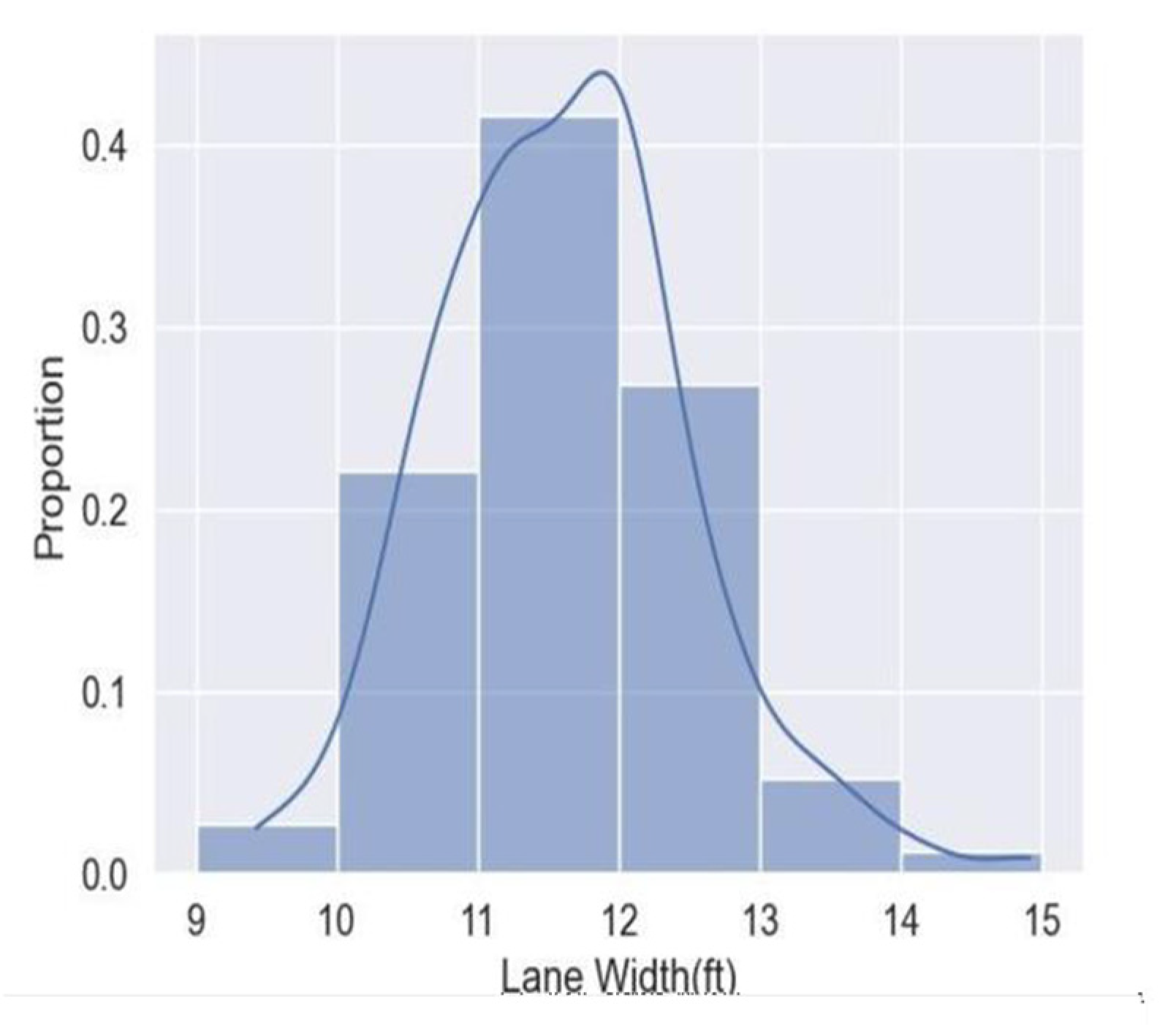
The correlation coefficient between the posted speed limit and the 85th percentile speed—a measure typically aligned with speed limit determinations—is 0.701 for urban sections. This indicates a reasonable level of correlation that supports the validity and reliability of StreetLight's speed data. Our primary independent variable of interest is lane width. As illustrated in Figure 4, the most prevalent roadway width in Utah is between 11 feet and less than 12 feet, with the next most common range being 12 feet to less than 13 feet.
Figure 1.
Lane Width Distribution of Urban and in the Collected Database
4. Results
4.1. Descriptive Statistics
To gain deeper insights into the database, we generated descriptive statistics in Table 4. In addition to the collected data, we added various dummy variables to the dataset to aid in modeling. These variables assume a value of 1 if present and 0 if absent. We also included and tested the natural logarithm of lane width, hypothesizing that the average speed may be nonlinearly related to these variables.
4.2. Modeling Speed
4.2.1. Linear Regression
Linear regression is a statistical method used to represent the relationship between a dependent variable and one or more independent variables. It assumes a linear relationship exists between the dependent and independent variables. Linear regression seeks to identify the optimal line or plane that characterizes the connection, facilitating the prediction of the dependent variable's value based on the values of the independent variables. This research utilized a multiple linear regression model to examine and forecast speed. The model allowed us to analyze the correlation between speed and several independent variables, including lane width, geometric factors, annual average daily traffic, and roadside elements. The association between each independent variable and the dependent variable is established by keeping all other variables in the regression equation constant.
4.2.2. Urban Arterial Speeds
The speed modeling started with a scatterplot of lane width vs. 85th percentile speed for UDOT urban arterials (see Figure 5). This dataset includes 320 roadway sections. There appears to be a weak but upward-sloping relationship between the two. The simple correlation coefficient between the two is 0.105, which is significant at the 0.065 level and short of the standard of 0.05. We would expect a correlation coefficient as large as lane widths by chance 6.5 percent of the time. The conventional significance level used in most statistical studies is 0.05, suggesting we would expect an effect this large by chance only 5 percent of the time (or for only one out of 20 random samples if there is no relationship between lane width and speed). Of course, this disregards the effect of any confounding variables, such as the number of lanes or the presence of a non-traversable median.
We then estimated multiple regression models using the urban area dataset. We found the most significant variables after estimating numerous regression models with different sets of variables available in our dataset.
We began by modeling the 50th percentile using StreetLight speed data. The 50th percentile speed is at or below 50 percent of the drivers traveling on a road section. It is the median speed of travel. The 50th percentile speed is taken from data collected during a 24-hour weekday. Controlling for other variables, the 50th percentile speed for our sample had a weak relationship to lane width. While the variable lane width had a positive sign, implying faster speeds with wider lanes (as expected), the significance level of lane width was 0.149, short of the standard 0.05 level.
Next, we modeled the 85th percentile speed for our independent variables, following the same procedure as for the 50th percentile or median speed, testing different independent variables. Traffic engineers and planners often use the 85th percentile speed to represent the upper end of the speed range. Posted speed limits are usually based on 85th percentile speeds. The results demonstrate that several variables, including lane width, significantly impact the 85th percentile speed driven on a given roadway section. In the final model, only statistically significant independent variables were retained.
The R2 is 0.405, meaning that the model explains more than 40 percent of the variance in the 85th percentile speed. We tested for multicollinearity, and there was none. The highest variance inflation factor (VIF) is 1.334, where values greater than 5.0 signal multicollinearity. We tested logged forms of the dependent and independent variables (the non-binary variables) with no significant change in results.
The lane width's significance level for the 85th percentile speed is 0.02, a result that would not be expected by chance. With a regression coefficient value of 1.012 compared to 0.674 in the 50th percentile speed model, lane width appears to have more impact on higher-speed traffic than typical speed traffic. Table 5 presents the best-fit regression model for the 85th percentile speed on UDOT urban arterials.
Following this logic, we decided to model the 95th percentile speed for our sample of UDOT urban arterials. The 95th percentile speed represents the uppermost end of the speed range and is also used by traffic engineers and transportation planners, though not as pervasively as the 85th percentile speed. The regression coefficient of lane width is 1.088, and the significance level is 0.011, showing again that lane width significantly impacts vehicle speed at the upper end of the speed range. Table 6 presents the best-fit regression model for the 95th percentile speeds on urban arterials.
Controlling for other variables, each additional foot of lane width increases the 85th percentile speed and the 95th percentile speed by more than one mph. The difference between a roadway with 14-foot lanes and 10-foot lanes would be more than four mph. This conclusion comes with caveats. First, our sample is significant but not that large. Second, our sample consists solely of state-owned and operated arterials in Utah. There is almost certainly less variance in the dataset than there would be if collectors or locally owned arterials were included. Third, while we tested for inter-rater reliability, there was an element of subjectivity in different raters' estimates of independent variables.
StreetLight speed data are also based on a sample, albeit a large one. Regarding the other variables, the number of lanes positively impacts speed. Specifically, the 85th percentile speed increases by 1.09 mph for each additional lane. Therefore, adding two lanes to a roadway (one in each direction) will increase about the same speed as increasing lane width by two feet. This observation has also been shown in road diet projects where fewer lanes result in lower speeds since the prudent driver sets the pace on the roadway with only one lane in each direction. A similar relationship is observed for block length within the roadway section. The results indicate that the longer the blocks along the roadway, the higher the midblock speed.
Conversely, non-traversable medians in a roadway can significantly reduce speed. Non-traversable medians are the most influential variable in reducing 85th-percentile speeds by 3.72 mph. The objects variable represents the extent of roadside objects alongside the roadway. Hence, it can be concluded that more buildings, trees, and other objects alongside a roadway section can reduce drivers' speed by nearly 3 mph. Sky Ahead has about two-thirds of this side effect. Additionally, the coefficient of on-street parking shows that the user's perception of the road can be influenced by side friction. Therefore, the "width" of the road is mainly influenced by drivers' perceptions, which affect the speed at which they drive.
It is important to note that the variables included in this model were selected after searching through all collected variables. The excluded variables either had unexpected signs or were insignificant in the roadway speed model. There was one exception. AADT per lane in thousands was one of those variables with a positive sign and a statistically significant p-value. Due to congestion, it was expected that the sign would be negative. Throughout 24 hours, congestion is not a factor in state urban arterials. Indeed, perhaps due to platooning, faster vehicles set the pace for slower vehicles.
4.3. Modeling Crashes
4.3.1. Count Regression Models
Traffic safety studies have employed various statistical models to analyze the relationship between cross-section design features and crash frequency, including Poisson and negative binomial models [28,30,60,61,62,63,64,65], zero-inflated negative binomial models [64,66,67], negative binomial models with random effects [64], Conway–Maxwell–Poisson generalized linear models [62], negative binomial models with random parameters [68], and dual-state negative binomial Markov switching models [69,70].
Our dependent variable is the crash count on a roadway section, excluding intersection crashes, as these are primarily influenced by conflicting movements at intersections rather than midblock speeds. When the outcome variable is a count with nonnegative integer values, many small values, and few large ones, two main analysis methods can be used: Poisson regression and negative binomial regression.
The Poisson and negative binomial models differ in their assumptions regarding the distribution of the dependent variable. Negative binomial regression is preferred when the dependent variable exhibits overdispersion, meaning the variance of the counts exceeds the mean. Overdispersion is commonly assessed using the Pearson and χ2 statistics, divided by the degrees of freedom, known as dispersion statistics. If these statistics exceed 1.0, the model is considered overdispersed. Based on these indicators, our data on crash counts show overdispersion, making the negative binomial model more suitable than the Poisson model for our analysis.
We started with three outcome variables—total crashes, injury crashes, and fatal crashes—but reduced it to two because fatal crashes are so rare. Only 3 percent of roadway sections in our sample experienced fatal crashes in 2021. Another statistical complication results from the fact that the variables of interest, crash counts and injury crash counts, were initially count variables for an entire section of roadway, each of varying length. Upon converting it to a total crash rate per mile and an injury crash rate per mile, the resultant output consisted of decimal values, which were subsequently rounded to restore the variable to its original count format, representing the total number of crashes and injury crashes per mile. This allowed us to apply a count model to the resulting dependent variable, the crash analysis norm.
A fourth statistical challenge is the excess of zero values in the injury count variable. While total crash counts on urban arterials generally follow a negative binomial distribution, 32% of urban sections report no injury crashes. To address this "zero inflation," a two-stage hurdle model is used. The first stage estimates a binary logistic regression to differentiate between sections with and without injury crashes. The second stage applies a negative binomial regression to estimate injury crashes for sections with any injury incidents. Each model was finalized after a thorough variable selection process, ensuring the expected signs were obtained.
4.3.2. Urban Arterial Crashes
The crash modeling started by estimating multiple models using the urban area dataset. This dataset includes 320 roadway sections, and the most significant variables were found after estimating numerous regression models with different sets of variables available in our dataset.
We began by modeling total crashes per mile, including property damage-only crashes (level 1 crashes from levels 1 to 5). Using negative binomial regression, the only variables that proved significant were the number of travel lanes and AADT per lane in thousands of vehicles. More travel lanes suggest more weaving in and out of traffic, as aggressive drivers change lanes often carelessly. The preceding discussion of road diets applies here. More AADT per lane in thousands suggests more exposure to potential crashes and less space between vehicles for crash avoidance. Notably, neither lane width nor 85th percentile speed (nor, parenthetically, 95th percentile speed) proved to be significant predictors of total crashes per mile. One could certainly imagine that lower-speed environments and the stop-and-go traffic accompanying them lead to more fender benders that offset more serious crashes in higher-speed environments. One could also imagine that narrower lanes cause drivers to exercise greater caution since the driving environment is less forgiving, one effect offsetting the other.
We next estimated a two-stage hurdle model for injury crashes per mile (level 2 through level 5). Hurdle modeling is a statistical technique for analyzing count data with many zero values. In such cases, traditional count models like Poisson or negative binomial regression may be inappropriate since they assume that the count variable follows a particular distribution and does not account for the excess zeros [71]. Hurdle modeling addresses this issue by breaking down the count data into two parts. A binary part represents the presence or absence of the event of interest (i.e., whether the count is zero), and a counting part represents the number of such events (i.e., positive counts). The binary part is modeled using binary logistic regression, while the count part is modeled using a truncated count model (e.g., zero-truncated Poisson or negative binomial regression). By separately modeling the binary and counting parts of the data, we attempt to account for the excess zeros in our crash data and improve the accuracy of the statistical analysis.
4.3.3. Binary Logistic Regression of Injury Crash Occurrence
Binary logistic regression is a statistical method that models the relationship between a binary dependent variable (with two possible outcomes) and one or more independent variables. The dependent variable is represented as a function of the independent variables by a logit function, which converts any real-valued input into a value ranging from 0 to 1. The logit function calculates the likelihood that the dependent variable assumes a specific value contingent upon the independent variables. Our hurdle model employs this methodology to analyze the correlation between the incidence or absence of crashes and other predictor factors.
Using the urban dataset, our optimal model for predicting injury crash occurrences incorporates lane width and the 85th percentile speed, together with the variables that demonstrated significance for total collision counts (refer to Table 7). Both are statistically significant at the 0.05 level and have positive coefficients. The correlation between velocity and injury-related collisions is evident. The correlation between lane width and injury crashes may be attributed to more prudent driver conduct when vehicles possess reduced clearance in multilane cross sections. The coefficient for lane width in the binary logistic model is 0.325, indicating that a one-unit (ft) increase in lane width correlates with an odds increase of a crash occurring by a factor of e raised to the power of 0.325, or 1.383. This is known as an odds ratio. A 1 ft increase in lane width correlates with a 38.3 percent rise in the probability of a route segment experiencing an injury collision. The p-value for this coefficient is 0.025, signifying statistical significance at a high confidence level. The coefficient for the 85th percentile speed in the binary logistic model is 0.046, indicating that a one-unit increase in lane width (mph) correlates with an increase in the probabilities of a crash by a factor of e raised to the power of 0.046, or 1.047. This is again termed an odds ratio. A one mph increase in the 85th percentile speed correlates with a 4.7 percent rise in the likelihood of an injury crash. The p-value for this coefficient is 0.012, signifying statistical significance at a high confidence level. Additional critical factors in the binary crash model are the number of lanes and the Average Annual Daily Traffic (AADT) per lane, measured in thousands. Both exhibit the anticipated good indicators. An increase in travel lanes indicates heightened weaving in traffic, as assertive drivers frequently alter their lanes. A higher AADT per lane indicates increased exposure to potential collisions and reduced spacing between vehicles for accident prevention.
4.3.4. Negative Binomial Regression
This analysis of injury crashes uses negative binomial regression within our hurdle model, following the adjustment for zero inflation (Table 8). We analyzed positive values of injury collisions. Only two independent variables demonstrated statistical significance: AADT (in thousands) and non-traversable median. Both lane width and 85th percentile speed were not statistically significant. This contradicts our previous finding that the incidence of injury crashes, treated as a binary variable, is associated with both lane width and the 85th percentile speed. The fundamental concept of a hurdle model is that various processes may influence the occurrence of an event, and if it occurs, so does the frequency of similar events. The anticipated number of crashes is just the product of the chance of a collision and the expected number of crashes, if applicable that occur. Consequently, it can be asserted with certainty that broader lanes on urban arterials correlate with increased injury crashes.
5. Discussion and Conclusions
In conclusion, this paper comprehensively studies the relationship between lane width, speed, and crash rates on urban arterial sections throughout Utah. The study comprises two key components: a thorough literature review investigating the effects of narrower travel lanes and geometric design features on speed, safety, and transportation impacts and statistical analyses examining various factors affecting roadway performance.
The literature review unequivocally confirms the potential impact of narrower travel lanes on speed, safety, and other transportation aspects. The statistical analyses yield significant findings for urban arterials. In urban areas, narrowing lane width leads to substantial reductions in vehicle speeds without increasing crash rates. The additional space gained from narrower lanes presents opportunities for implementing various safety and pedestrian-friendly enhancements. Consequently, we recommend revising the current minimum lane width standard, particularly in low-speed, highly urbanized areas, and potentially exploring further reductions in specific cases while considering exceptions for areas with heavy truck traffic.
The speed models demonstrate the significant influence of lane width on speed for urban arterials, with narrower lanes consistently associated with lower speeds. Other variables, such as the number of lanes, non-traversable medians, on-street parking density, roadside objects, and average block length, also impact speed on urban arterials.
This study provides compelling evidence supporting the feasibility and safety advantages of reducing lane widths on Utah's urban arterials. These findings give transportation policymakers and practitioners valuable insights into shaping lane width policies to enhance road safety and operational performance. Narrower lanes free up space for other uses, such as bike lanes and median refuge islands. However, further research with larger sample sizes in rural areas is essential to deepen our understanding of safety impacts. Implementing the recommended revisions can potentially optimize Utah's transportation infrastructure, accommodating diverse users while ensuring safer roadways for all.
Author Contributions
Conceptualization, R.E.; investigation, B.A., W.Y., N.P., H.K., and N.T.; data curation, B.A., W.Y., N.P., H.K., and N.T.; writing—original draft preparation, B.A., W.Y., N.P., H.K., and N.T.; writing—review and editing, R.E. and W.Y.; supervision, R.E.; funding acquisition, R.E. All authors have read and agreed to the published version of the manuscript. All authors have read and agreed to the published version of the manuscript. .
Funding
This research was funded by the Utah Department of Transportation, grant number 22-8095—“Transportation benefits and costs of reducing lane widths on urban and rural arterials.
Data Availability Statement
Dataset available on request from the authors.
Conflicts of Interest
The authors declare no conflicts of interest.
References
- Swift, P.; Painter, D.; Goldstein, M. Residential Street Typology and Injury Accident Frequency. Congress for the New Urbanism, Denver, Co. USA 1997.
- Abdel-Rahim, A.; Sonnen, J. Potential Safety Effects of Lane Width and Shoulder Width on Two-Lane Rural State Highways in Idaho. 2012, 52p.
- Pokorny, P.; Jensen, J.K.; Gross, F.; Pitera, K. Safety Effects of Traffic Lane and Shoulder Widths on Two-Lane Undivided Rural Roads: A Matched Case-Control Study from Norway. Accid Anal Prev 2020, 144, 105614. [CrossRef]
- Rahman, Z.; Memarian, A.; Madanu, S.; Iqbal, G.; Anahideh, H.; Mattingly, S.P.; Rosenberger, J.M. Assessment of the Impact of Lane Width on Arterial Crashes. Journal of Transportation Safety and Security 2018, 10, 229–250. [CrossRef]
- Rista, E.; Goswamy, A.; Wang, B.; Barrette, T.; Hamzeie, R.; Russo, B.; Bou-Saab, G.; Savolainen, P.T. Examining the Safety Impacts of Narrow Lane Widths on Urban/Suburban Arterials: Estimation of a Panel Data Random Parameters Negative Binomial Model. Journal of Transportation Safety and Security 2018, 10, 213 – 228. [CrossRef]
- Godley, S.T.; Triggs, T.J.; Fildes, B.N. Perceptual Lane Width, Wide Perceptual Road Centre Markings and Driving Speeds. Ergonomics 2004, 47, 237–256. [CrossRef]
- Manuel, A.; El-Basyouny, K.; Islam, Md.T. Investigating the Safety Effects of Road Width on Urban Collector Roadways. Saf Sci 2014, 62, 305–311. [CrossRef]
- Potts, I.B.; Harwood, D.W.; Richard, K.R. Relationship of Lane Width to Safety on Urban and Suburban Arterials. Transp Res Rec 2007, 63–82. [CrossRef]
- Ahmed, M.; Huang, H.; Abdel-Aty, M.; Guevara, B. Exploring a Bayesian Hierarchical Approach for Developing Safety Performance Functions for a Mountainous Freeway. Accid Anal Prev 2011, 43, 1581–1589. [CrossRef]
- P; Ande, A.; Abdel-Aty, M. A Novel Approach for Analyzing Severe Crash Patterns on Multilane Highways. Accid Anal Prev 2009, 41, 985–994. [CrossRef]
- Zhu, H.; Dixon, K.K.; Washington, S.; Jared, D.M. Predicting Single-Vehicle Fatal Crashes for Two-Lane Rural Highways in Southeastern United States. Transportation Research Record: Journal of the Transportation Research Board 2010, 2147, 88–96. [CrossRef]
- Nowakowska, M. Logistic Models in Crash Severity Classification Based on Road Characteristics. Transportation Research Record: Journal of the Transportation Research Board 2010, 2148, 16–26. [CrossRef]
- Gårder, P. Segment Characteristics and Severity of Head-on Crashes on Two-Lane Rural Highways in Maine. Accid Anal Prev 2006, 38, 652–661. [CrossRef]
- Dumbaugh, E. Design of Safe Urban Roadsides. Transportation Research Record: Journal of the Transportation Research Board 2006, 1961, 74–82. [CrossRef]
- Hauer, E.; Council, F.M.; Mohammedshah, Y. Safety Models for Urban Four-Lane Undivided Road Segments. Transp Res Rec 2004, 96–105. [CrossRef]
- Strathman, J.G.; Dueker, K.J.; Zhang, J.; Williams, T. Analysis of Design Attributes and Crashes on the Oregon Highway System.; 2001; Vol. 2;.
- Parsons Transportation Group Relationship Between Lane Width and Speed Review of Relevant Literature. 2003, 1–6.
- Harwood W, D. Effective Utilization of Street Width on Urban Arterials; 1990; ISBN 0-309-04853-2.
- Dumbaugh, E.; Gattis, J.L. Safe Streets, Livable Streets. Journal of the American Planning Association 2005, 71, 283–300. [CrossRef]
- Hauer, E. Lane Width and Safety. Literature. 2000.
- Bobermin, M.P.; Silva, M.M.; Ferreira, S. Driving Simulators to Evaluate Road Geometric Design Effects on Driver Behaviour: A Systematic Review. Accid Anal Prev 2021, 150, 105923. [CrossRef]
- Ewan, L.; Al-Kaisy, A.; Hossain, F. Safety Effects of Road Geometry and Roadside Features on Low-Volume Roads in Oregon. Transp Res Rec 2016, 2580, 47–55. [CrossRef]
- Gargoum, S.A.; El-Basyouny, K. Exploring the Association between Speed and Safety: A Path Analysis Approach. Accid Anal Prev 2016, 93, 32–40. [CrossRef]
- Bamzai, R.; Lee, Y.; Li, Z. SAFETY IMPACTS OF HIGHWAY SHOULDER ATTRIBUTES IN ILLINOIS; 2011;
- Gitelman, V.; Doveh, E.; Carmel, R.; Hakkert, S. The Influence of Shoulder Characteristics on the Safety Level of Two-Lane Roads: A Case-Study. Accid Anal Prev 2019, 122, 108–118. [CrossRef]
- Arévalo-Támara, A.; Orozco-Fontalvo, M.; Cantillo, V. Factors Influencing Crash Frequency on Colombian Rural Roads. Promet - Traffic - Traffico 2020, 32, 449–460. [CrossRef]
- Gross, F.; Jovanis, P.P. Estimation of the Safety Effectiveness of Lane and Shoulder Width: Case-Control Approach. J Transp Eng 2007, 133, 362–369. [CrossRef]
- Abdel-Aty, M.A.; Radwan, A.E. Modeling Traffic Accident Occurrence and Involvement. Accid Anal Prev 2000, 32, 633–642. [CrossRef]
- Council, F.M.; Stewart, J.R. Safety Effects of the Conversion of Rural Two-Lane to Four-Lane Roadways Based on Cross-Sectional Models. Transp Res Rec 1999, 35–43. [CrossRef]
- Milton, J.; Mannering, F. The Relationship among Highway Geometrics, Traffic-Related Elements and Motor-Vehicle Accident Frequencies. Transportation (Amst) 1998, 25, 395–413. [CrossRef]
- Ma, J.; Kockelman, K.M. Poisson Regression for Models of Injury Count, by Severity. Transportation Research Record: Journal of the Transportation Research Board 2006, 24–34.
- Park, J.; Abdel-Aty, M.; Wang, J.-H.; Lee, C. Assessment of Safety Effects for Widening Urban Roadways in Developing Crash Modification Functions Using Nonlinearizing Link Functions. Accid Anal Prev 2015, 79, 80–87. [CrossRef]
- Imprialou, M.I.M.; Quddus, M.; Pitfield, D.E.; Lord, D. Re-Visiting Crash-Speed Relationships: A New Perspective in Crash Modelling. Accid Anal Prev 2016, 86, 173–185. [CrossRef]
- Biswas, S.; Chandra, S.; Ghosh, I. Effects of On-Street Parking in Urban Context: A Critical Review. Transportation in Developing Economies 2017, 3, 1–14. [CrossRef]
- Krieger, A.; Lennertz, W. Andres Duany and Elizabeth Plater-Zyberk : Towns and Town-Making Principles; Harvard University Graduate School of Design, 1991;
- De Cerreño, A.L.C. Dynamics of On-Street Parking in Large Central Cities. Transp Res Rec 2004, 130–137. [CrossRef]
- Ossenbruggen, P.J.; Pendharkar, J.; Ivan, J. Roadway Safety in Rural and Small Urbanized Areas. Accid Anal Prev 2001, 33, 485–498. [CrossRef]
- Søren, B.; Jensen, U. Road Safety and Perceived Risk of Cycle Facilities in Copenhagen. Presentation to AGM of European Cyclists Federation 2007, 1–9.
- Kraidi, R.; Evdorides, H. Pedestrian Safety Models for Urban Environments with High Roadside Activities. Saf Sci 2020, 130, 104847. [CrossRef]
- Edquist, J.; Rudin-Brown, C.M.; Lenné, M.G. The Effects of On-Street Parking and Road Environment Visual Complexity on Travel Speed and Reaction Time. Accid Anal Prev 2012, 45, 759–765. [CrossRef]
- Harvey, C.; Aultman-hall, L. Urban Streetscape Design and Crash Severity. 2015, 1–8. [CrossRef]
- Moradi, A.; Saeed, S.; Nazari, H.; Rahmani, K. Sleepiness and the Risk of Road Traffic Accidents : A Systematic Review and Meta-Analysis of Previous Studies. Transportation Research Part F: Psychology and Behaviour 2019, 65, 620–629. [CrossRef]
- Young, K.L.; Salmon, P.M. Examining the Relationship between Driver Distraction and Driving Errors : A Discussion of Theory , Studies and Methods. Saf Sci 2012, 50, 165–174. [CrossRef]
- Naderi, J.R. Landscape Design in Clear Zone Effect of Landscape Variables on Pedestrian Health and Driver Safety. Transportation Research Record: Journal of the Transportation Research Board 2003, 1851, 119–130. [CrossRef]
- Ewing, R.; Handy, S. Measuring the Unmeasurable : Urban Design Qualities Related to Walkability Measuring the Unmeasurable : Urban Design Qualities Related to Walkability. 2009. [CrossRef]
- Potts, I.B.; Harwood, D.W.; Richard, K.R. Relationship of Lane Width to Safety on Urban and Suburban Arterials. Transp Res Rec 2007, 63–82. [CrossRef]
- Ewing, R.; Yang, W.; Promy, N.S.; Kaniewska, J.; Tabassum, N. Selective State DOT Lane Width Standards and Guidelines to Reduce Speeds and Improve Safety. Infrastructures (Basel) 2024, 9, 141. [CrossRef]
- Shao, C.Q.; Rong, J.; Liu, X.M. Study on the Saturation Flow Rate and Its Influence Factors at Signalized Intersections in China. Procedia Soc Behav Sci 2011, 16, 504–514. [CrossRef]
- Susilo, B.H.; Solihin, Y. Modification of Saturation Flow Formula by Width of Road Approach. Procedia Soc Behav Sci 2011, 16, 620–629. [CrossRef]
- Chen, P.; Nakamura, H.; Asano, M. Saturation Flow Rate Analysis for Shared Left-Turn Lane at Signalized Intersections in Japan. Procedia Soc Behav Sci 2011, 16, 548–559. [CrossRef]
- Shao, C.Q.; Rong, J.; Liu, X.M. Study on the Saturation Flow Rate and Its Influence Factors at Signalized Intersections in China. Procedia Soc Behav Sci 2011, 16, 504–514. [CrossRef]
- Susilo, B.H.; Solihin, Y. Modification of Saturation Flow Formula by Width of Road Approach. Procedia Soc Behav Sci 2011, 16, 620–629. [CrossRef]
- Chandra, S.; Kumar, U. Effect of Lane Width on Capacity under Mixed Traffic Conditions in India. J Transp Eng 2003, 129, 155–160. [CrossRef]
- FHWA Road Diets (Roadway Reconfiguration); 2010;
- Gudz, E.M.; Fang, K.; Handy, S.L. When a Diet Prompts a Gain Impact of a Road Diet on Bicycling in Davis, California. Transp Res Rec 2016, 2587, 61–67. [CrossRef]
- Ntonifor, C. THESIS TITLE: Valuation of The Impacts of Road Diet Implementation: Wilson Boulevard Road Diet, Arlington County Virginia.
- Anderson, G.; Searfoss, L. Safer Streets, Stronger Economies. Smart Growth America 2015, 40.
- Liu, C.; Zhao, M.; Li, W.; Sharma, A. Multivariate Random Parameters Zero-Inflated Negative Binomial Regression for Analyzing Urban Midblock Crashes. Anal Methods Accid Res 2018, 17, 32 – 46. [CrossRef]
- Chen, T.; Sze, N.N.; Chen, S.; Labi, S. Urban Road Space Allocation Incorporating the Safety and Construction Cost Impacts of Lane and Footpath Widths. J Safety Res 2020, 75, 222–232. [CrossRef]
- Hadi, M.A.; Aruldhas, J.; Chow, L.F.; Wattleworth, J.A. Estimating Safety Effects of Cross-Section Design for Various Highway Types Using Negative Binomial Regression. Transp Res Rec 1995, 169–177.
- Jones, B.; Janssen, L.; Mannering, F. Analysis of the Frequency and Duration of Freeway Accidents in Seattle. Accid Anal Prev 1991, 23, 239–255. [CrossRef]
- Lord, D.; Park, P.Y.J. Investigating the Effects of the Fixed and Varying Dispersion Parameters of Poisson-Gamma Models on Empirical Bayes Estimates. Accid Anal Prev 2008, 40, 1441–1457. [CrossRef]
- Poch, M.; Mannering, F. Negative Binomial Analysis of Intersection-Accident Frequencies. J Transp Eng 1996, 122, 105–113. [CrossRef]
- Shankar, V.; Mannering, F.; Barfield, W. Effect of Roadway Geometrics and Environmental Factors on Rural Freeway Accident Frequencies. Accid Anal Prev 1995, 27, 371–389. [CrossRef]
- Zhao, J.; Liu, Y.; Wang, T. Increasing Signalized Intersection Capacity with Unconventional Use of Special Width Approach Lanes. Computer-Aided Civil and Infrastructure Engineering 2016, 31, 794–810. [CrossRef]
- Carson, J.; Mannering, F. The Effect of Ice Warning Signs on Ice-Accident Frequencies and Severities. Accid Anal Prev 2001, 33, 99–109. [CrossRef]
- Lee, J.; Mannering, F. Impact of Roadside Features on the Frequency and Severity of Run-off-Roadway Accidents: An Empirical Analysis. Accid Anal Prev 2002, 34, 149–161. [CrossRef]
- Anastasopoulos, P.C.; Mannering, F.L. A Note on Modeling Vehicle Accident Frequencies with Random-Parameters Count Models. Accid Anal Prev 2009, 41, 153–159. [CrossRef]
- Malyshkina, N. V.; Mannering, F.L. Zero-State Markov Switching Count-Data Models: An Empirical Assessment. Accid Anal Prev 2010, 42, 122–130. [CrossRef]
- Malyshkina, N. V.; Mannering, F.L. Empirical Assessment of the Impact of Highway Design Exceptions on the Frequency and Severity of Vehicle Accidents. Accid Anal Prev 2010, 42, 131–139. [CrossRef]
- McDowell, A. From the Help Desk: Hurdle Models. The Stata Journal: Promoting communications on statistics and Stata 2003, 3, 178–184. [CrossRef]
Figure 1.
Example of Open Streetscape(a) and Enclosed Streetscape(b) (Sourced from Aultman-hall & Harvey, 2015).
Figure 1.
Example of Open Streetscape(a) and Enclosed Streetscape(b) (Sourced from Aultman-hall & Harvey, 2015).
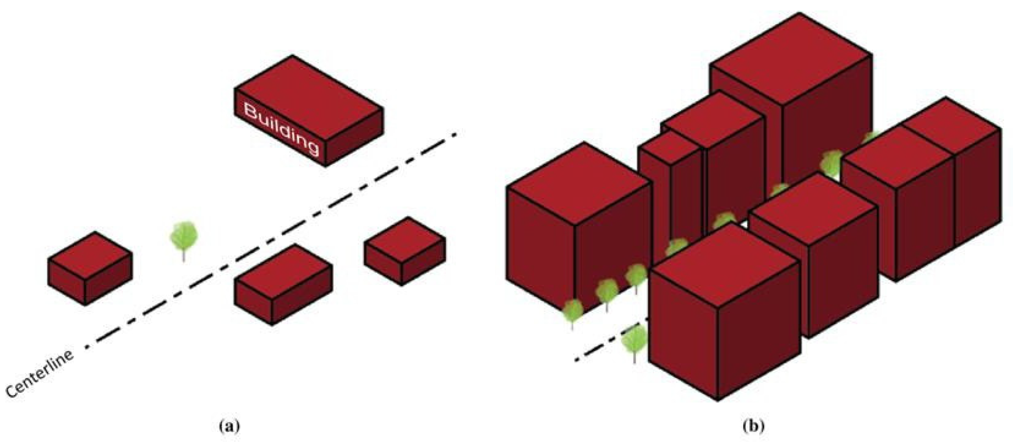
Figure 2.
Geographic Map of Study Sections.
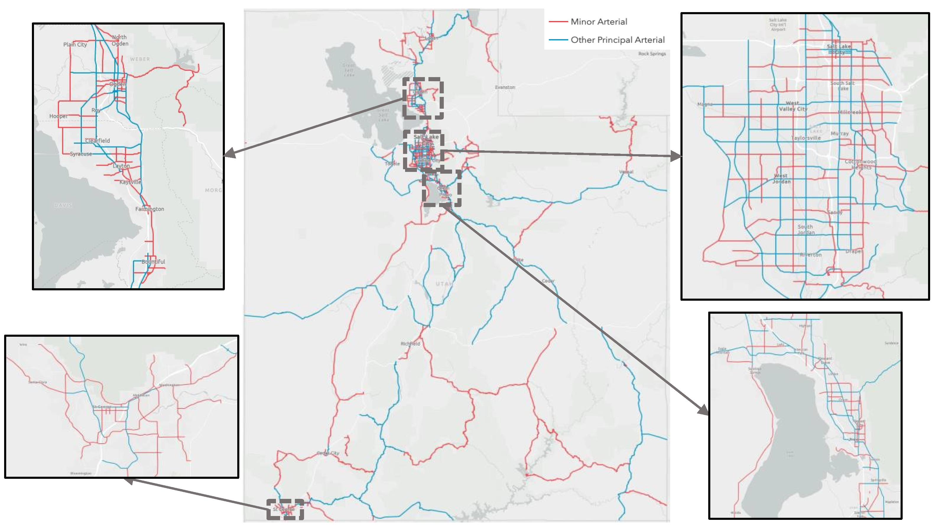
Figure 3.
Inter-rater Reliability Test Results for Cronbach's Alpha.
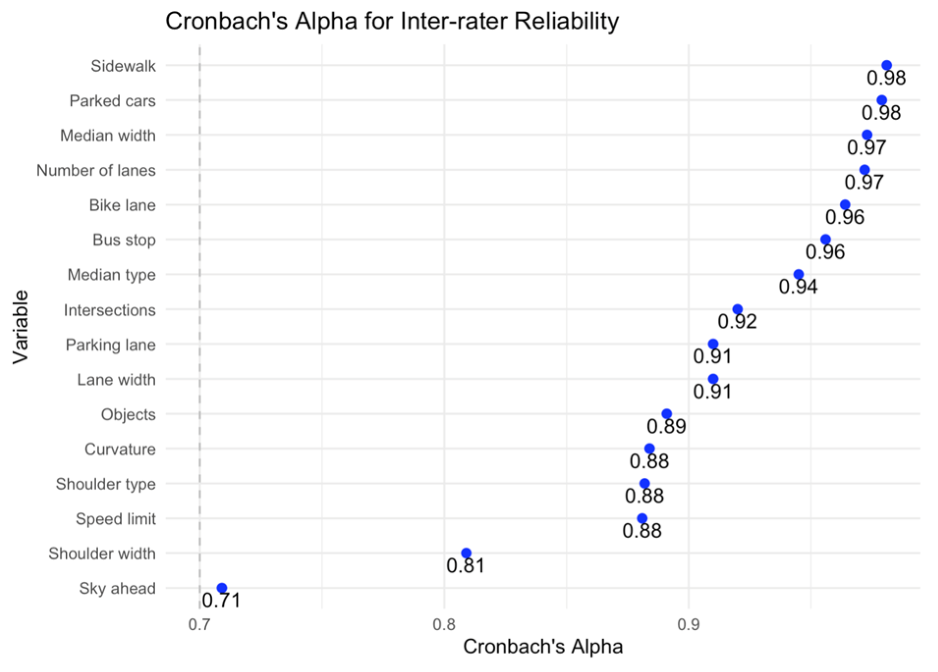
Figure 5.
Scatterplot of Lane Width (in ft) vs. 85th Percentile Speed (in mph) for UDOT Urban Arterials.
Figure 5.
Scatterplot of Lane Width (in ft) vs. 85th Percentile Speed (in mph) for UDOT Urban Arterials.
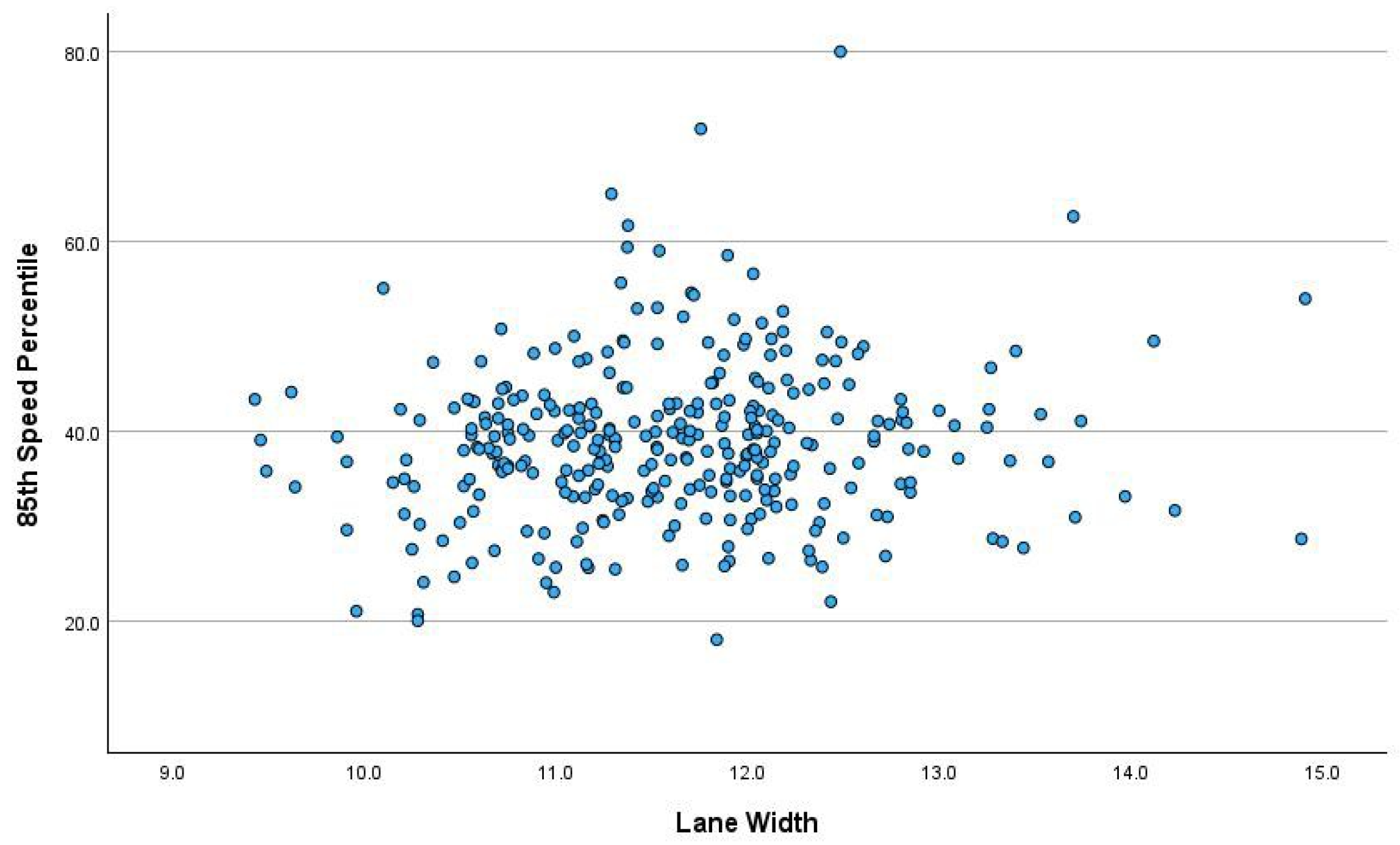

Table 1.
Descriptive Statistics of Roadway Study Sections.
| Count | Mean | Median | Min. | Max. | S.D. |
| Average Length (Miles) | 0.79 | 0.63 | 0.05 | 5.13 | 0.56 |
| Average Lane Width(ft) | 11.90 | 11.98 | 9.5 | 21.11 | 0.75 |
Table 2.
Units of Analysis and Characteristics.
| Analysis units | Method 1: Midblock segments | Method 2: Sections of road |
|
Unit characteristics |
- Total number of units: 4,125 - Mean length: 0.9 mi. - Range: 0.1 to 35mi. 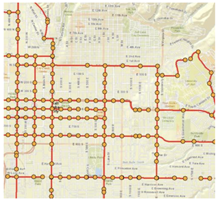
|
- Total number of units: 1,869 - Mean length: 2.0 mi. - Range: 0.1 to 49.3 mi. 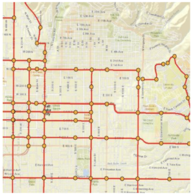
|
|
Data collection time |
- Relatively shorter time per sample | - Relatively longer to examine multiple midblock segments |
|
Number of crashes |
- Zero-crash samples: 16% (644 out of 4,125) of the total cases - Mean crashes per unit: 14 - Range: 0 to 355 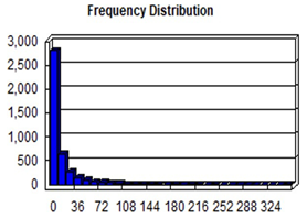
|
- Zero-crash samples: 5% (85 out of 1,869) of the total cases - Mean crashes per unit: 31 - Range: 0 to 355 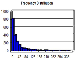
|
Table 3.
Observation Protocol for Identifying Homogenous Roadway Sections.
| Criteria | Observation Protocol |
| Number of lanes | The count of through lanes in both directions was tracked, eliminating flush medians and turning lanes adjacent to intersections. Any alteration in the number of lanes was recorded as "0," but a consistent lane design was recorded as "1." |
| Posted speed limit | A change in the speed limit was recorded as "0," and a uniform speed limit was recorded as "1." |
| Lane width | Lane width was measured at multiple random points along the section. A difference greater than 1 ft was recorded as "0," and a uniform lane width was recorded as "1." |
| Median width/type | Any significant changes in median width (e.g., from 12 ft to 13 ft) or changes in median type (e.g., from traversable to non-traversable) have been recorded as "0." A constant median was documented as "1." |
| Shoulder width/type | Any significant changes in shoulder width (e.g., from 2 ft to 3 ft) or shoulder type (e.g., present in one direction and absent in the other) were recorded as "0." A consistent shoulder was recorded as "1." |
| Sidewalk | Any significant changes in the presence of sidewalks (e.g., from present to absent) were recorded as "0." Consistency in sidewalk presence was recorded as "1." |
| Bike lane | For the presence of bike lanes, if there is any significant change (e.g., from present to absent), it is recorded as 0. If the condition remains uniform across the section, it is recorded as 1. |
Table 4.
Statistical Distribution of Collected Data for Arterial Sections in Urban Areas.
| Variable | Mean | STD | Min | 25% | 50% | 75% | Max |
| Length (miles) | 0.57 | 0.29 | 0.13 | 0.32 | 0.51 | 0.80 | 1.51 |
| Lane Width (ft) | 11.62 | 0.90 | 9.43 | 11.01 | 11.63 | 12.11 | 14.91 |
| Lane ≥ 12 ft (dummy) | 0.34 | 0.47 | 0.0 | 0.0 | 0.0 | 1.0 | 1.0 |
| Ln (Lane Width) | 2.45 | 0.08 | 2.24 | 2.40 | 2.45 | 2.49 | 2.70 |
| Num. Lanes | 3.96 | 1.38 | 2.0 | 4.0 | 4.0 | 4.0 | 8.0 |
| Median (dummy) | 0.80 | 0.40 | 0.0 | 1.0 | 1.0 | 1.0 | 1.0 |
| Nontraversable Median (dummy) |
0.19 | 0.40 | 0.0 | 0.0 | 0.0 | 0.0 | 1.0 |
| Median Width (ft) | 10.86 | 7.02 | 0.00 | 8.97 | 12.30 | 14.07 | 41.73 |
| Shoulder (dummy) | 0.68 | 0.47 | 0.0 | 0.0 | 1.0 | 1.0 | 1.0 |
| Shoulder Width (ft) | 6.43 | 5.40 | 0.00 | 0.00 | 6.71 | 10.61 | 31.62 |
| Sidewalk (dummy) | 0.93 | 0.26 | 0.0 | 1.0 | 1.0 | 1.0 | 1.0 |
| Bike Lane (dummy) | 0.19 | 0.39 | 0.0 | 0.0 | 0.0 | 0.0 | 1.0 |
| Bus Stop (dummy) | 0.60 | 0.49 | 0.0 | 0.0 | 1.0 | 1.0 | 1.0 |
| Parking Lane (dummy) | 0.03 | 0.18 | 0.0 | 0.0 | 0.0 | 0.0 | 1.0 |
| Num. Parked Cars | 6.04 | 15.68 | 0.00 | 0.00 | 0.00 | 4.25 | 169.00 |
| Parked Cars (/Mile) | 12.84 | 33.11 | 0.00 | 0.00 | 0.00 | 9.76 | 362.02 |
| Curve Length (ft) | 3041.70 | 1548.27 | 699.61 | 1705.15 | 2682.23 | 4334.57 | 7995.77 |
| Euclidean Length (ft) | 3017.45 | 1528.49 | 700.83 | 1639.08 | 2677.24 | 4268.39 | 8036.47 |
| Curvature (degree) | 1.01 | 0.14 | 0.79 | 1.00 | 1.00 | 1.00 | 3.37 |
| Sky Ahead | 0.75 | 0.44 | 0.0 | 0.0 | 1.0 | 1.0 | 1.0 |
| Objects | 0.79 | 0.41 | 0.0 | 1.0 | 1.0 | 1.0 | 1.0 |
| Intersections | 3.56 | 2.96 | 0.0 | 1.0 | 3.0 | 5.0 | 15.0 |
| Block Length (mi) | 0.16 | 0.13 | 0.02 | 0.09 | 0.13 | 0.18 | 1.04 |
| Speed Limit (mph) | 38.30 | 6.54 | 25.0 | 35.0 | 40.0 | 40.0 | 70.0 |
| AADT (in 1000s) | 22.85 | 11.37 | 0.99 | 14.42 | 20.80 | 30.08 | 61.09 |
| AADT (in 1000s per lane) | 5.80 | 2.15 | 0.25 | 4.44 | 5.55 | 7.06 | 13.63 |
| 50th Percentile Speed | 29.69 | 8.75 | 3.00 | 24.35 | 29.67 | 34.49 | 62.90 |
| 85th Percentile Speed | 38.56 | 8.66 | 13.00 | 33.65 | 38.38 | 42.79 | 80.00 |
| 95th Percentile Speed | 43.70 | 8.29 | 23.81 | 38.56 | 43.07 | 47.05 | 89.00 |
| All Crash Count | 6.06 | 6.61 | 0.0 | 1.0 | 4.0 | 8.0 | 41.0 |
| Injury Crash Count | 1.88 | 2.45 | 0.0 | 0.0 | 1.0 | 3.0 | 16.0 |
| Fatal Crash Count | 0.04 | 0.21 | 0.0 | 0.0 | 0.0 | 0.0 | 2.0 |
| All Crash Count (/Mile) | 11.01 | 11.72 | 0.0 | 3.0 | 7.5 | 15.0 | 83.0 |
| Injury Crash Count(/Mile) | 3.34 | 3.95 | 0.0 | 0.0 | 2.0 | 4.3 | 26.0 |
| Fatal Crash Count(/Mile) | 0.05 | 0.028 | 0.0 | 0.0 | 0.0 | 0.0 | 2.0 |
Table 5.
Linear Regression Model for 85th Percentile Speeds on UDOT Urban Arterials.
| Variable | Coefficient | Std. error | t-statistic | p-value |
| (Intercept) | 16.689 | 5.666 | 2.945 | 0.003*** |
| Lane width (ft) | 1.012 | 0.431 | 2.346 | 0.020*** |
| Number of lanes | 1.090 | 0.303 | 3.602 | <0.001*** |
| Non-traversable median (dummy) | -3.720 | 1.060 | -3.508 | 0.001*** |
| Parked cars (/mile) | -0.041 | 0.011 | -3.607 | <0.001*** |
| Sky ahead (dummy) | 2.004 | 0.937 | 2.139 | 0.033** |
| Objects* | -2.789 | 0.985 | -2.832 | 0.005*** |
| Block length (ft) | 0.005 | 0.001 | 8.919 | <0.001*** |
| AADT (in 1000s per lane) | 0.650 | 0.172 | 3.779 | <0.001*** |
| R2 | 0.405 | |||
*Significance < 0.01***, <0.05**, 0.1*.
Table 6.
Linear Regression Model for 95th percentile Speeds on UDOT Urban Arterials.
| Variable. | Coefficient | Std. error | t-statistic | p-value |
| (Intercept) | 20.809 | 5.620 | 3.703 | <0.001*** |
| Lane width (ft) | 1.088 | 0.428 | 2.543 | 0.011** |
| Number of lanes | 1.282 | 0.300 | 4.271 | <0.001*** |
| Non-traversable median (dummy) | -3.953 | 1.052 | -3.759 | <0.001*** |
| Parked cars (/mile) | -0.041 | 0.011 | -3.621 | <0.001*** |
| Sky ahead (dummy) | 1.808 | 0.929 | 1.947 | 0.052* |
| Objects (dummy) | -3.282 | 0.977 | -3.360 | 0.001*** |
| Block length (ft) | 0.005 | 0.001 | 8.982 | <0.001*** |
| AADT (in 1000s per lane) | 0.591 | 0.170 | 3.467 | 0.001*** |
| R2 | 0.421 | |||
*Significance < 0.01***, <0.05**, 0.1*.
Table 7.
Binary Model of Injury Crash Occurrence in Urban Areas.
| Variable | Coefficient | Std. error | Wald statistic | p-value | exp (Coeff) |
| (Constant) | -7.674 | 1.891 | 16.464 | <0.001*** | 0.000 |
| Lane width (ft) | 0.325 | 0.145 | 5.025 | 0.025** | 1.383 |
| Number of lanes | 0.331 | 0.102 | 10.477 | 0.001*** | 1.393 |
| AADT per lane | 0.295 | 0.069 | 18.195 | <0.001*** | 1.343 |
| 85th percentile speed | 0.046 | 0.018 | 6.282 | 0.012** | 1.047 |
| pseudo R2 | 0.204 | ||||
*Significance < 0.01***, <0.05**, 0.1*.
Table 8.
Negative Binomial Regression Model of Urban Injury Crashes.
| Variable | Coefficient | Std. error | Z-value | p-value |
| (Constant) | -0.91 | 2.90 | -0.31 | 0.750 |
| AADT (in 1000) | 0.03 | 0.00 | 6.30 | <0.001*** |
| 85th percentile speed (mph) | 0.04 | 0.07 | 0.48 | 0.630 |
| Lane width (ft) | 0.17 | 0.24 | 0.71 | 0.480 |
| Non-traversable median | -0.39 | 0.12 | -3.29 | <0.001*** |
| Number of lanes | 0.07 | 0.05 | 1.58 | 0.111 |
*Significance < 0.01***, <0.05**, 0.1*.
Disclaimer/Publisher’s Note: The statements, opinions and data contained in all publications are solely those of the individual author(s) and contributor(s) and not of MDPI and/or the editor(s). MDPI and/or the editor(s) disclaim responsibility for any injury to people or property resulting from any ideas, methods, instructions or products referred to in the content. |
© 2024 by the authors. Licensee MDPI, Basel, Switzerland. This article is an open access article distributed under the terms and conditions of the Creative Commons Attribution (CC BY) license (http://creativecommons.org/licenses/by/4.0/).
Copyright: This open access article is published under a Creative Commons CC BY 4.0 license, which permit the free download, distribution, and reuse, provided that the author and preprint are cited in any reuse.


