Submitted:
07 December 2024
Posted:
09 December 2024
You are already at the latest version
Abstract
The UK retail landscape has undergone significant changes over the past decade, driven by factors such as the rise of online shopping, economic downturns, and, more recently, the COVID-19 pandemic. Accurately measuring pedestrian flows in retail areas with high spatial and temporal resolution is essential for selecting the most suitable forecast model for different retail locations. However, several studies have adopted a one-solution-fits-all approach, overseeing important local characteristics only sometimes captured by the best global model. In this work, we investigate the optimal forecasting method to predict pedestrian footfall in diverse retail areas in Great Britain. After reviewing six representative time series forecasting models, our results indicate that the LSTM model outperforms traditional methods in most areas. However, pedestrian counts at certain locations with particular spatial characteristics are better forecasted with other algorithms.
Keywords:
Forecasting
; Human mobility
; Footfall
1. Introduction
Functional characteristics of urban areas and local activity patterns are some of the main factors that dictate the suitability of a site for a store location on very granular scales [1,2]. The development of retailing also depends largely on changes in pedestrian flow, which cannot be understood simply as exploring the regional footfall pattern. Footfall (FF) plays an important role here, serving as a proxy for the activity and vitality of retail areas [3].
High street footfall can easily fall despite the population growth, and this was seen to be the case during the 2008 economic downturn, as Genecon reports a 10% footfall decline in the UK high streets, excluding Central London (2008–2011) [4]. In consequence, footfall, as such, can be used as a more accurate and up-to-date measure of the potential customer base around retail areas on a daily or weekly basis, helping retailers plan business activities, such as scheduling the opening/ close time and personnel, production, and transportation, or formulate long-term business plans, such as risk management [5,6]. Footfall prediction can also help the government take emergency measures in advance to prevent overcrowding and reduce crowd risk. For example, overcrowding in Oxford Street, the world’s biggest high street, led to temporary tube station closures 113 times in 2015 [7]. Especially in the context of the global COVID-19 pandemic, the risk of overcrowding has expanded to more than physical injuries. In other words, footfall research is a prerequisite for any business.
However, the existing research on crowd flow prediction mainly focuses on short-term crowd behaviour modelling at the micro level. For example, Zhang et al. proposed a cellular automata model for simulating pedestrian flow [8]. Liu et al. introduced a graph convolutional network (GCN) to predict the crowd flow in a walking street [9]. Therefore, from a theoretical point of view, there is an important gap in the prediction of footfall in retail areas on a large scale due to the limitation of data acquisition in the past. Traditionally, forecasting models focused on AR and MA have been considered among the most accurate forecasting approaches in over a half-century [10]. More recently, and acknowledging the shortcomings of such parametric models, several studies have introduced the non-parametric approaches based on ML algorithms on the forecasting of temporal datasets [11,12] since they do not presuppose the nature of time series distribution. Empirical research has shown that ML models perform quite well on temporal data forecasting and usually outperform the statistical approaches [13,14,15,16]. Parmezan et al. applied various indicators, including MSE, Theil’s U coefficient, POCID, and a multi-criteria performance measure, to evaluate the prediction performance of statistical and ML models. They demonstrated that the SARIMA model is the only statistical time series prediction model that performs better than some ML models on several datasets [17]. However, another comparative study by Gautam and Singh indicates that parametric models are competitive with ML models and perform better for some datasets evaluated by symmetric mean absolute percentage error (sMAPE) [18]. Finally, Han et al. conducted a comparative study on the prediction performance of various models on both generated and real-world data, adopting traditional ML models as benchmarks and MAE together with MAPE as accuracy indicators. Results indicate that XGBoost, LSTM, and hybrid models produce stable predictions [19].
In this work, using data from a network of Wi-Fi sensors at retail locations across Great Britain, we applied different time series forecasting methods to analyse the pedestrian flow in hundreds of retail areas. We identified the behaviour of each model concerning specific spatiotemporal locations to provide a comprehensive guide for users to choose the optimal models for predicting footfall in retail areas.
The research question addressed here is: What is the optimal pedestrian flow forecasting approach for retail areas in Great Britain? In an attempt to answer the research question, this paper also aims to address the following objectives:
- What are the most commonly used and best-performing time series prediction models for pedestrian flow forecasting? How do we compare the performance of different forecasting models?;
- Does the best forecasting model differ for different retail areas in GB?
- Is the difference among the optimal footfall prediction approaches related to some spatial characteristics of different locations?
The rest of this paper is structured as follows: First, in the methods section, we discuss, analyse, and assess the footfall dataset compared with other human mobility datasets freely available. Then, we discuss the forecasting methods employed in this work, providing different metrics to evaluate their accuracy. Then, in the discussion section, we evaluate the statistical and spatial distribution of the footfall counts related to their spatial location and their influence on the accuracy of the different forecasting methods. Finally, we elaborate on conclusions, recommendations, and possible paths to extend this research.
This study can be used as a reference for future research on pedestrian flow prediction in GB retail areas.
2. Materials and Methods
Figure 1 shows our workflow to analyse the FF data, define different FF forecasting model and relate them to the street type and output area classification around each location to understand why some methods performed better that others depending on the location. In the rest of this section, we elaborate on each one of these components.
Datasets
While retail geographical analysis has been covered in previous research [20,21], the analysis and prediction of pedestrian dynamics within large sample locations based on recorded activity patterns on a finer temporal scale is scarce. Research of micro-scale retail geography based on the demand side could only be conducted through manual surveying in the past, which required a costly and laborious process and without continuous data acquisition. However, these shortcomings have been addressed since the rapid development and wide-scale application of smartphones, Wi-Fi, GPS, and Bluetooth technologies. The Consumer Data Research Centre (cdrc.ac.uk), in collaboration with the Local Data Company (www.localdatacompany.com), set up the SmartStreetSensor project for collecting and analysing Wi-Fi probe requests where a network of Wi-Fi sensors has been installed in retail establishments across the UK, including shopping centres, out-of-town retail parks and urban town centres [22].
Several studies have used this data for a wide range of applications[3,23,24,25]. Particularly, the research of Lugomer [3] demonstrated that the footfall patterns in retail areas exhibit different dynamic characteristics on different days of the week.
The footfall data comprises more than 1000 Wi-Fi Sensors attached to retail areas across the UK, with the vast majority in London (Figure 2).
The project employs a proprietary sensor network that records mobile device signals to discover available Wi-Fi access points. Once captured, the data is processed into five-minute aggregated counts, and each record has the following structure: sensor, timestamp, footfall count, location, device, and address (latitude, longitude). We refer the reader to [26] for the full technical definition.
Figure 3 illustrates the time series of average footfall counts in Great Britain retail areas. The footfall shows a dramatic fluctuation since 2020 due to the COVID-19 epidemic. In addition, the data for some dates from September to October 2019 are missing due to technical issues in the data collection process.
Data Pre-Processing
Since it’s hard to avoid various technical problems of Wi-Fi sensors attached to each location during the data acquisition period, such as power outages or accidental damage, the footfall data is somehow inconsistent within most areas, which needs to be filtered and interpolated at the first stage. Moreover, the 5-minute interval for the original aggregated footfall contains significant white noise interference. Therefore, to reduce the amount of calculation and improve the prediction accuracy, the interval of footfall data used in forecasting must be appropriately expanded.
The original footfall data was resampled for one hour, and the missing data was interpolated linearly. To avoid the influence of the COVID-19 pandemic and missing data, the selected time frame for this study was from January 2018 to August 2019. Later in this section, we will discuss splitting the dataset into two groups: training and testing data. For now, it is worth mentioning that locations with more than 40% of missing data in the training set or more than 20% of missing data in the test set were removed. After this data-cleaning procedure, 314 locations were used in this work.
2.1. Footfall Data as Time Series
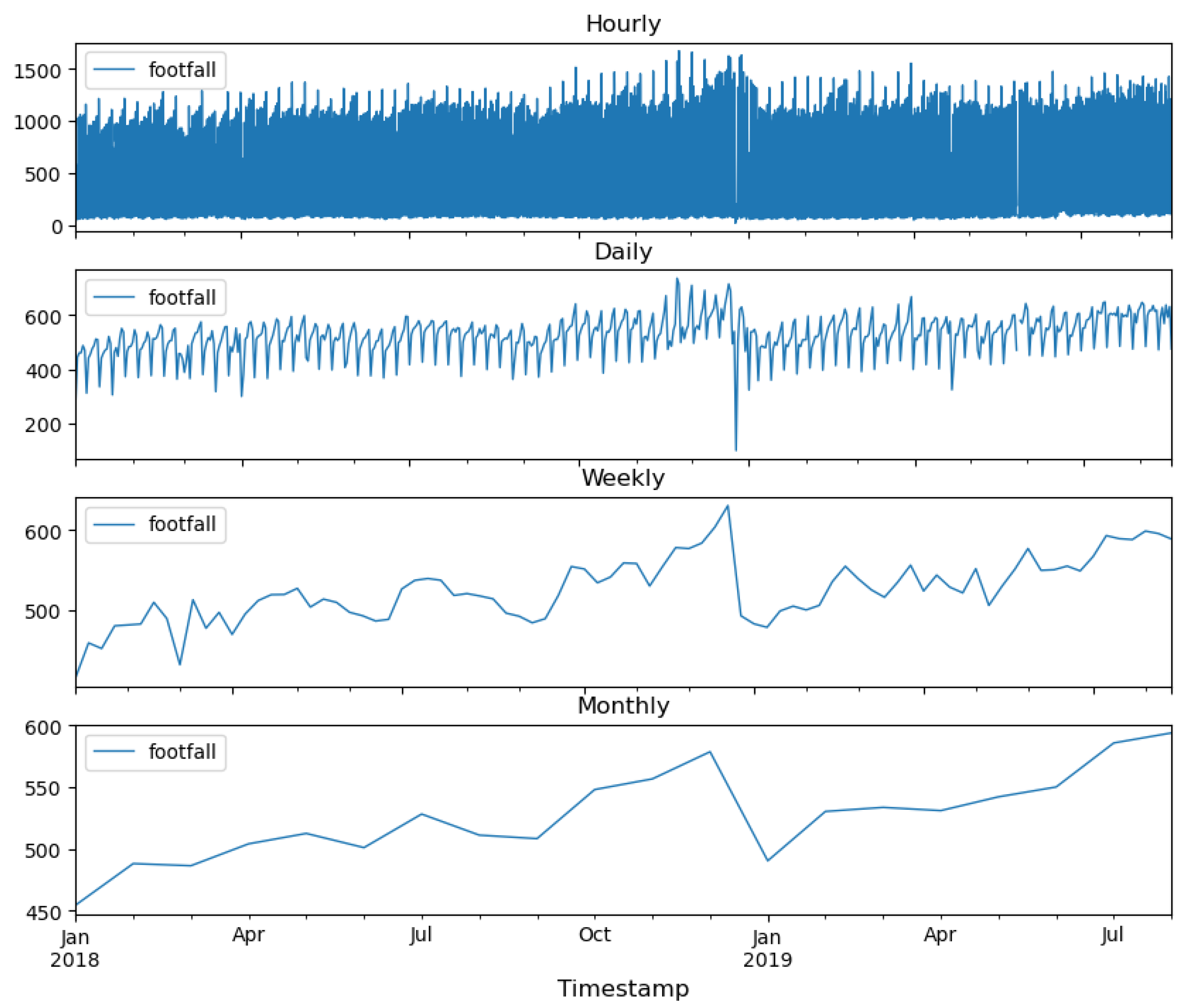
Figure 5 shows the FF data as a Time Series aggregated by different seasonalities. The sharp decay after December 26 is clear in all panels, while during Easter week, the fall in FF is only observable at precisely the Weekly aggregation.
Figure 4 illustrates the average hourly distribution of footfall on a different day of the week, which shows a strong similarity in pattern between Monday to Thursday, compared with Friday, Saturday, and Sunday, which show a distinct distribution.
Figure 4.
Hourly footfall distribution. (a) by day of the week. (b) footfall counts.
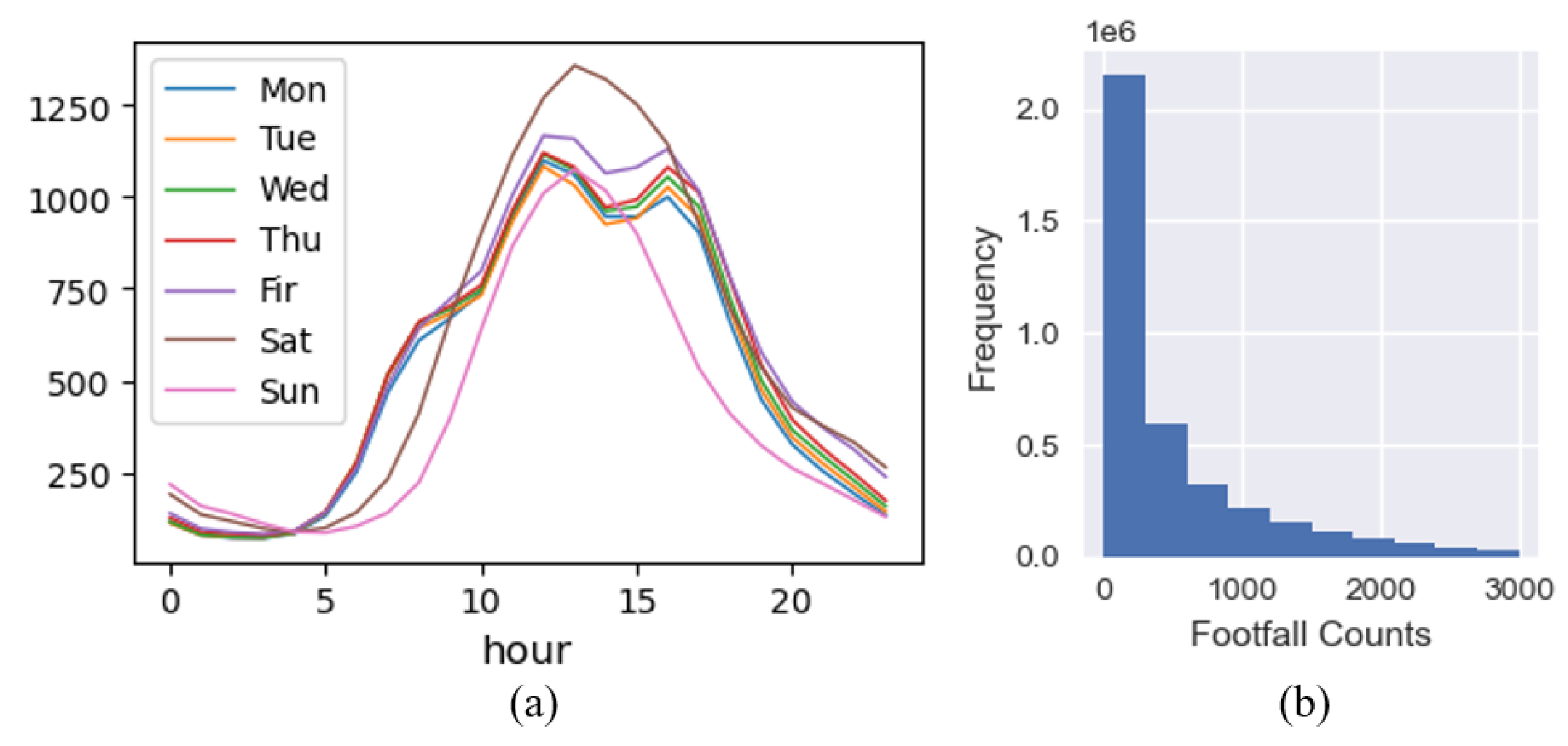
Figure 5.
Footfall time series after cleansing.
Assessment
The FF signal’s trend and seasonal components (Figure 5) depict the non-random nature of this data, and that is detecting the ups and downs in FF activity around different retail locations. To further assess these features, we compared our data with three external sources measuring human activity: 1) extraordinary events, 2) public transport figures, and 3) Google popular times.
Extraordinary Events
The Notting Hill Carnival is a massive yearly event in London that attracts thousands of visitors over three days. 2018, the carnival occurred from Saturday, the 25th, to Monday, August 27.
No sensor is installed around Nothing Hill tube station. Still, there are two locations around High Street Kensington station, location 709 and location 957, which are popular locations for getting into the event. Figure 6 shows the change between an average Monday and Carnival Monday of location 709 in 2018. In the former, the typical morning/afternoon peaks at rush hour, plus a peek at lunchtime, are clear, while on Carnival day, there is only one peak at 2 pm and from 10 am to 5 pm, the volume of FF is in orders of more than 1,500 people per hour. The data captured by these sensors successfully detect the change in FF around this area due to the unusual amount of activity and pedestrian flows.
The second, easy-to-spot event is the decline in FF due to the COVID-19 pandemic. After the outbreak of the pandemic, public transport journeys were severely affected by the soaring number of cases; from Feb 2020 to May 2020 and from Oct 2020 to Feb 2021, there were two cliff-like drops in public traffic journeys, which coincided with two major lockdowns of London. By inspecting Figure 6, we can observe how it practically disappeared from the graph during the first major lockdown in the UK (March 2022).
Public Transport
We related the FF counts to the entry and exit figures for nearby underground stations to assess whether these sensors capture the activity trends around different areas. The data is open source, reported by the Transport for London (TfL) authority [27].
The annual counts for the London underground are collected and represent each day in autumn each year. Therefore, the footfall data for September, October and November 2018 is adopted for comparison. We conducted a simple Pearson correlation analysis of locations vs stations (Figure 7) over 88 retail areas where the distance location-station is less than one kilometre. The results indicate that the distribution of FF counts on different weekdays (Monday to Thursday, Friday, Saturday, and Sunday) is highly similar to the passenger counts of nearby tube stations, with a median correlation coefficient greater than 0.8.
In Appendix A, we showed an example of a particular popular station in London, Piccadilly Circus, to further show the value of the FF data. We also refer the reader to Appendix A for the Google Popular Times comparison.
Convert Format
After conducting the coordinate and projection conversion in the ArcGis software, the Euclidean Distance to roads and Output Area information were calculated and attached to each location.
Join Spatial Characteristics
To associate FF locations with their urban environment, we joined the footfall data with:
- Open Road Data from Digimap, Ordnance Survey (digimap.edina.ac.uk). The data offers a high-level view of the road network with generalised geometry and network connectivity in Great Britain.
- Output Areas 2011 Classification from the CDRC (data.cdrc.ac.uk/dataset/output-area-classification-2011). The 2011 Classification for Output Areas (2011 OAC) is a hierarchical geodemographic classification across the UK that identifies areas of the country with similar characteristics that contain the following breakdown of Output Areas into different groups and sub-groups.
2.2. Pedestrian Footfall Prediction
Before applying any forecasting methods, the standard approach is to split the dataset into training and test datasets. In this work, the training set was split from January 1/1/2018, to July 28/08/2019, and the validation set was split from July 29/08/2019 for three weeks.
Classic Forecasting Methods
The approaches for time series forecasting [28,29] rely on the basic idea that historical data contains intrinsic patterns which convey the key information for the future description of the phenomenon investigated. Nevertheless, these patterns are usually non-trivial to identify, and their discovery becomes one of the primary goals of time series processing: the features the patterns found will repeat and which sort of changes they might suffer over time [30]. This idea led to the decomposition of the time series components, namely trend, seasonality, cyclic and residuals, which form the basis of many classic time series decomposition methods. Time series forecasting methods can be categorized by whether to use parameters as parametric or non-parametric methods [18], or by methodology as statistical and machine learning (ML) models [31]
The classic methods employed in this work are:
It is worth mentioning that the literature about these methods is vast. In this work, we refer to [33] to develop these classical models.
Machine Learning Approaches
There is a close connection between the nature of time series forecasting and the regression analysis of the ML classification. The classic support vector machine [37], Bayesian network [38] and Gaussian process [39] have all achieved good results in time series forecasting. The early artificial neural network (ANN) is also used to obtain the long-term trend in time series. With the rise of neural networks, deep learning can also be regarded as an effective tool for forecasting time series.
Long Short-Term Memory Model (LSTM)
The LSTM recurrent network [40] is a special Recurrent Neural Network (RNN) designed to solve the traditional RNN problem when dealing with long-series data-designed gradient disappearing problems. By introducing a three-gating mechanism, a forget, input, and output gate, the flow of information is controlled through a single LSTM unit. This model has been successfully applied in time series analysis, classification and prediction [40,41,42] in both univariate and multivariate domains [43]
The standard gate system, as described in [44], has the following logic:
- Forget the door (Forget Gate): Forget door step determines the time before memory in the current time step needs to be forgotten.
-
Input Gate: The input gate determines how much of the current input information will be kept in the memory cell.The updated formula of the memory content is:
- Memory cell state update: The state of the memory cell at the current time step is determined by both the results of the forget Gate and the input gate:
-
Output (Output door Gate): The output door step determines the time to hide the status update, which is the final output of the LSTM hidden state.The update formula for the hidden state is:
Together, these gates and the cell state form a complex memory system that allows LSTM to effectively process sequential data, making them well-suited for tasks like time series forecasting. In summary, the model determines which information from the previous time step is relevant and should be retained and which information can be discarded. Second, it learns new information from the current input and integrates it with the retained information. Finally, it outputs a portion of its updated state to the next time step. This entire process constitutes a single-time step in the LSTM.
Identifying the Optimal Forecasting Method
To statistically identify forecast accuracy equivalence for two sets of predictions, we applied the Diebold-Mariano (DM) Test [45]. With the assumption that the difference between the first list of predictions and the actual values is and the second list of forecasts and the actual value is . The length of the time series is T. Then d can be defined based on different criteria (crit), whereas in the measure of MSE,
The null hypothesis is , and the test statistics follow the student-T distribution with degree of freedom .
The DM test is adopted to identify whether the forecasts of the two prediction methods have a significant distinction.
Spatial Distribution Analysis
This part of the analysis mainly adopts the classification approaches to explore whether the different results of the optimal prediction method of locations are related to some spatial characteristics, that is, the relationship with roads and land type.
The Random Forests (RF) algorithm represents a family of models involved in building an ensemble of decision trees, where each tree is formed through a bootstrap sample of the data. Then, each tree node is split according to the best of a subset of randomly chosen predictors [46]. Moreover, the outputs from each tree are averaged to obtain an ensemble prediction of the target variable that can be used as classification tools [47].
The RF model could help identify spatial factors highly correlated with the optimal prediction method of retail locations and illustrate the influence of different factors quantitatively.
3. Results
Optimal Prediction Methods Statistics
The results shown in Table 1 confirm that the LSTM prediction model is the optimal method with the lowest RMSE for 83.76% of locations, where 76.81% of the predictions meet the DM test, which means the LSTM model outperforms other prediction methods on footfall forecasts within 64.33% of all locations with a statistical significance.
The rest of the methods only account for a small proportion of the total, not exceeding 1.6%. In addition, Figure 8 indicates the MA approach does not perform well in predicting incomplete datasets.
To further study the prediction performance of other statistical time series prediction models, we counted the times each method performs best, excluding the LSTM model and those that satisfy the DM test.
Table 2 illustrates that MA, as the best prediction method with the lowest RMSE, has the most significant proportion among different locations, followed by SARIMA and HW, and the Naïve approach holds a minor proportion.
However, the number of the best prediction methods for different locations that meet the DM test only accounts for half of the total, meaning that half of the locations simultaneously have more than one optimal prediction method. As a result, different forecasting methods have no significant difference in the distribution of predicted pedestrian footfall in these retail areas. In addition, Figure 9 indicates these statistical approaches show little preference for datasets with different missing data ratios. Still, it should be noted that HW and MA locations show the smallest missing data ratio in both Figure 8 and Figure 9.
Pedestrian Footfall Distribution
Figure 10 shows the average footfall distribution of locations with different optimal methods by hourly, weekly, and monthly.
Figure 10a indicates significant hourly distribution differences among these locations. The average hourly change is the most stable within locations where SARIMA is the optimal model. It also has the most negligible total flow, compared with locations with the best predicting method LSTM with the highest average footfall, which can also be seen in the weekly and monthly figures. The peak of the average hourly flow of locations with the optimal method HW appears later in the day.
Figure 10b shows locations where MA is the optimal method have a more significant peak on Saturday in the average weekly footfall distribution. Also, the peak of locations with SARIMA appears on Friday, which is different from other locations. It can be seen from Figure 10c that locations with HW or MA as the best forecasting method show a more apparent seasonal trend in the average monthly footfall distribution, compared with Naïve, SARIMA and LSTM.
However, it should be noted that, except for locations where the optimal prediction method is LSTM, the number of other locations is relatively small, so the analysis of the results could be affected by some exceptional cases and might not be universal.
Spatial Characteristics
To try to make sense of the differences observed in best forecasting method among some locations, we used the datasets listed in Section 2.1.
Distance to Different Types of Roads
Figure 11 illustrates the average Euclidean Distance from classified locations to different types of roads.
Results indicate that locations with SARIMA, the optimal method, are closest to the main roads, including the A road and the B road, compared with the LSTM locations with the longest average Distance to the A road and the Naïve locations with the longest average Distance to the B road. In addition, The HW locations are nearest to the local roads. Also, the MA locations have the longest Distance to local roads and access roads, compared with the SARIMA locations close to the local roads and access roads. It can be seen from Figure 20 that Naïve locations have the longest average Distance to the motorway, compared with the MA locations that are closest to the motorway.
Output Area Classification
Figure 12 illustrates the land classification counts by different locations. Results show that cosmopolitans, densely populated urban areas where most of the population live, account for the largest proportion in most locations except for Naïve locations. In addition, LSTM locations cover a wide variety of land types.
Multi-Relationships with Spatial Factors
Figure 13 shows the correlation matrix of continuous variables. No significant correlation among variables was observed.
The RF classifier model is not well-fitted for predicting the optimal method for each location through spatial characteristic variables. The training accuracy is 0.98, and the test accuracy is 0.61. Results shown in Figure 14 indicate that the optimal footfall prediction method of locations relates more to the Distance between locations on different roads. – We need to consider presenting this part as it is quite important, but it is a whole new paper
At Appendix B we showed a particular case of study for two locations on a famous high street in London, Oxford Circus.
4. Discussion
Results of the comparison among the performance of different prediction models show that the performance of the LSTM model is the most stable, even in retail areas where the LSTM is not the optimal footfall forecasting model, the prediction error is relatively small, which means that the LSTM model has a very good fit for the pedestrian flow prediction in all sorts of retail areas across the UK.
Other forecasting models apply to certain types of footfall data with different time series characteristics.
For example, in areas where the Naïve approach performs well, the flow distribution varies greatly in different periods within the research time range. This may be due to recent changes in the external environment that have affected the flow of people in a local area, resulting in a footfall distribution similar to a random walk time series. -Laura’s paper - where can the random walk be trusted? The daily footfall distribution for MA locations has three distinctive peaks in the morning, noon, and evening. The distribution on weekdays is also different from other areas. For example, compared with other locations where Saturday is the highest pedestrian flow peak in a week, the peak in MA locations appears earlier on Friday. Moreover, the overall time series in the MA locations tends to be more stable, with no obvious trend at a large scale.
The footfall distribution in locations where the HW model performs well is similar to SARIMA locations. The difference is mainly in the distribution on working days. Within a week, the pedestrian flow changes in the SARIMA areas are more dramatic. Similarities in performance between HW and SARIMA models might be related to the common features shared among ES and ARIMA models. A statistical framework introduced by Geurts, Box and Jenkins indicates that the predictions produced by some linear ES models serve as a particular case of ARIMA [36].
The differences in footfall distribution in these retail areas might also be related to their spatial characteristics, indirectly leading to differences in optimal forecasting methods for locations. Therefore, this study mainly explores the differences in land and road types of locations with different optimal prediction methods.
To a certain extent, the statistical analysis explained the differences in the pedestrian flow distribution in these retail areas.
Locations with Naïve the optimal method are relatively farther from B roads and motorways and closer to minor roads and local access roads. The spatial characteristics of MA locations are just the opposite of the Naïve locations.
The spatial characteristics of HW and SARIMA locations are quite similar regarding their relations to traffic distribution. The only difference is that SARIMA locations are farther away from A and B roads. In contrast, HW locations are closer to them.
However, the RF model does not fit well, which means that the pedestrian flow characteristics/optimal prediction method of one certain retail location might be related to more sophisticated spatial characteristics.
Limitations
Reflecting on the optimal pedestrian flow forecasting approach for retail areas in Great Britain, our results have demonstrated that it differs in different locations despite the LSTM model being best for most areas. However, some limitations on the data and methodology have yet to be addressed.
One limitation is that the predictive performance might be related to the division of the test set for different locations. However, this shortcoming can be solved by introducing cross-validation, which requires a large amount of calculation and a sufficiently long time series period.
Another limitation is the need for more sample size. Although the LDC has installed over a thousand Wi-Fi sensors to capture pedestrian footfall in Great Britain, due to technical problems, only 311 locations can be used for prediction. At the same time, the more complex spatial features behind these locations need to be excavated.
In terms of the train/test split, future work could introduce cross-validation to identify the best prediction approach and make the conclusion more general. Different forecast periods could also be considered, corresponding to actual uses.
5. Conclusions
This research employs a comparative study approach to identify the optimal footfall prediction method in retail areas across Great Britain. This work responds to the need to further explore the footfall dataset in GB retail areas, especially in forecasting the temporal pedestrian dynamics, which has great practical importance for retailing in different formats in making business decisions as well as helping the government take emergency measures in advance to reduce the crowd risk. A simulation study has been conducted to compare the statistics and machine learning models. To conduct the empirical comparison, 5-time series prediction methods are selected, namely the Naïve, Moving Averages, Holt-Winters, SARIMA, and LSTM. In addition, MSE and Diebold-Mariano tests are used to test the forecasting performance. A significant statistical difference is shown in the footfall time series and spatial characteristics of locations classified through their optimal footfall forecasting methods.
However, it is acknowledged that future work and improvements could be undertaken in several ways. Multiple variables, such as precipitation and temperature, could be introduced to reduce even further the prediction error in modelling the pedestrian flow. Other trending time series forecasting models achieve good results; for example, fbProphet, the open-source algorithm of Facebook, performs well in dealing with outliers and missing values [48].
Finally, in recent years, the XGBoost model [49] has gain notoriety for its efficiency, flexibility and scalability capabilities, making it widely applicable to classification, regression, and ranking tasks. A key advantage of XGBoost is its proficiency in handling complex relationships. The input features in this study include only one variable which is the main reason to exclude this popular model from this study.
Author Contributions
Conceptualization, Y.W. and R.M.; methodology, R.M.; software, Y.W.; validation, R.M., Y.W.; resources, Y.W. and R.M.; data curation, Y.M.; writing —original draft preparation, Y.W.; writing—review and editing, R.M.; supervision, R.M. All authors have read and agreed to the published version of the manuscript.
Funding
This research received no external funding.
Data Availability Statement
The footfall data presented in this article is not readily available because the CDRC labelled as Safeguarded data: data to which access is restricted due to license conditions, but where data are not considered ‘personally-identifiable’ or otherwise sensitive (from: https://data.cdrc.ac.uk/protecting-data). Access is available via a remote service with registration and project approval requirements (https://data.cdrc.ac.uk/using-our-data-services) The road network presented in this article is not readily available because the Digimap Collections (https://digimap.edina.ac.uk/) provide maps and mapping data to UK colleges and universities. Institutions should subscribe to the service so their members can access the data (https://digimap.edina.ac.uk/help/about/eligibility/). The road network could be obtained from open sources, such as OpenStreetMap, and it would make no difference in the results obtained. The Output Area Classification (2011) is open data provided by the CDRC. The data is available at https://data.cdrc.ac.uk/dataset/output-area-classification-2011.
Acknowledgments
We acknowledge the support of the CDRC in approving our application for the footfall data.
Conflicts of Interest
The authors declare no conflicts of interest.
Appendix A. Assessment
Appendix A.1. Picadilly Circus Underground Station
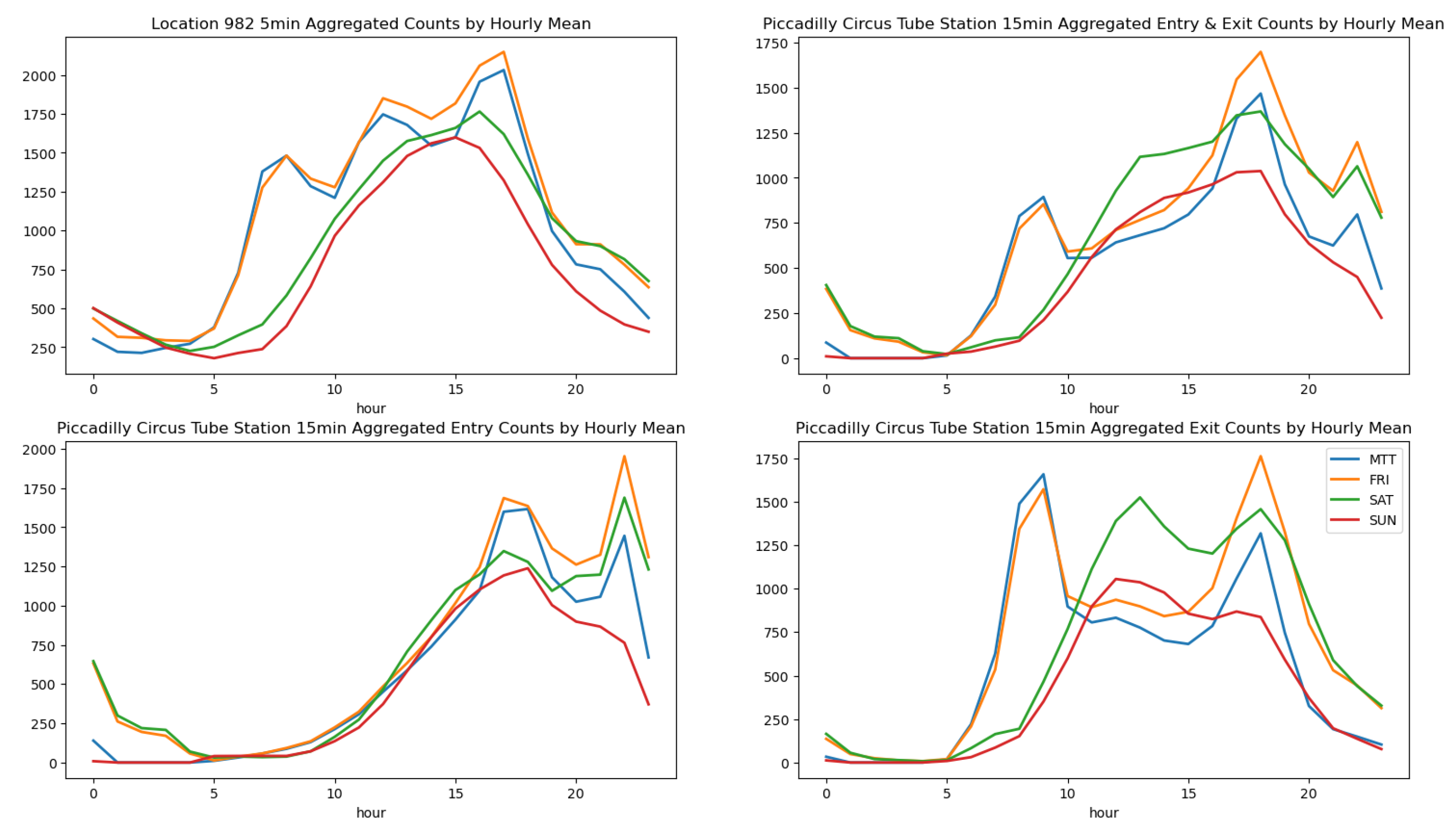
In Figure A1, the correlation between the two is more significant on weekends. However, for some well-known large retail areas, the distribution of footfall on weekends might be more related to the number of tube exits.
Figure A1.
Hourly footfall distribution of location 982 and nearby tube station flows.
Appendix A.2. Google Popular Times
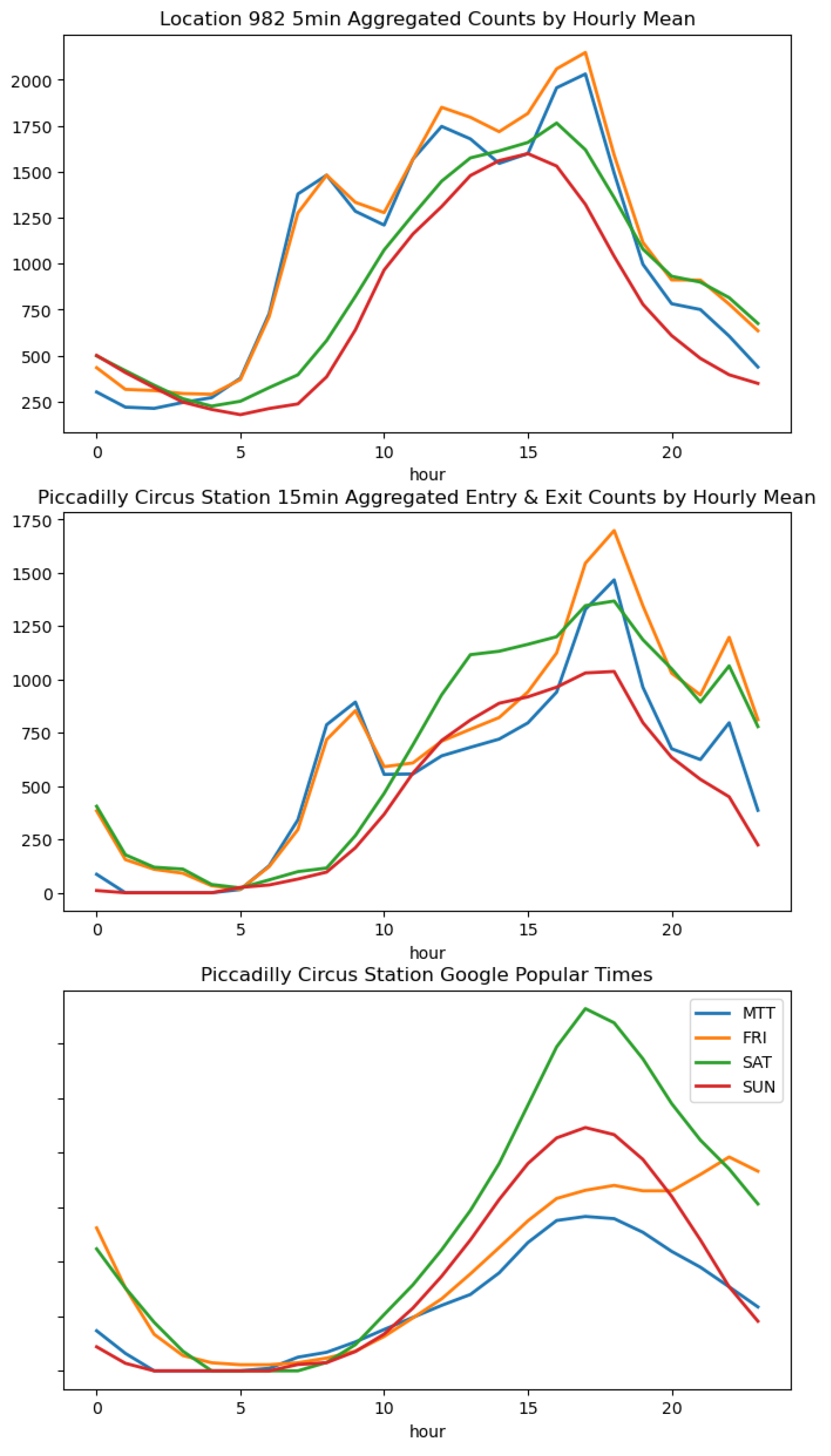
The distribution of the pedestrian flow of 6 selected retail areas in autumn 2018 is somewhat similar to the popular times of the Google map, with the overall median of Pearson correlation higher than 0.7. The differences in correlations across weekdays are also similar to the TfL data in that the correlation on weekends is higher than on workdays, which is reflected in Figure A2. Location 982 on Regent Street is about 100 metres from the Piccadilly Circus station. As seen from Figure A3, the pedestrian flow data shows similar troughs and peaks at around 5 am and 5 pm, respectively. However, due to the differences in the data acquisition time (Google Weekly popular Times uses an annual average and is updated to 2022), it can be seen that the pedestrian flow of some stations has undergone significant changes, which is mainly reflected in the decrease in the ratio of passengers on weekdays and the decrease in morning rush hour.
Figure A2.
Box plot of Pearson correlation of FF in retail areas and Google popular times of nearby tube station on different days of the week. The MTT label refers to Monday-Thursday.
Figure A2.
Box plot of Pearson correlation of FF in retail areas and Google popular times of nearby tube station on different days of the week. The MTT label refers to Monday-Thursday.
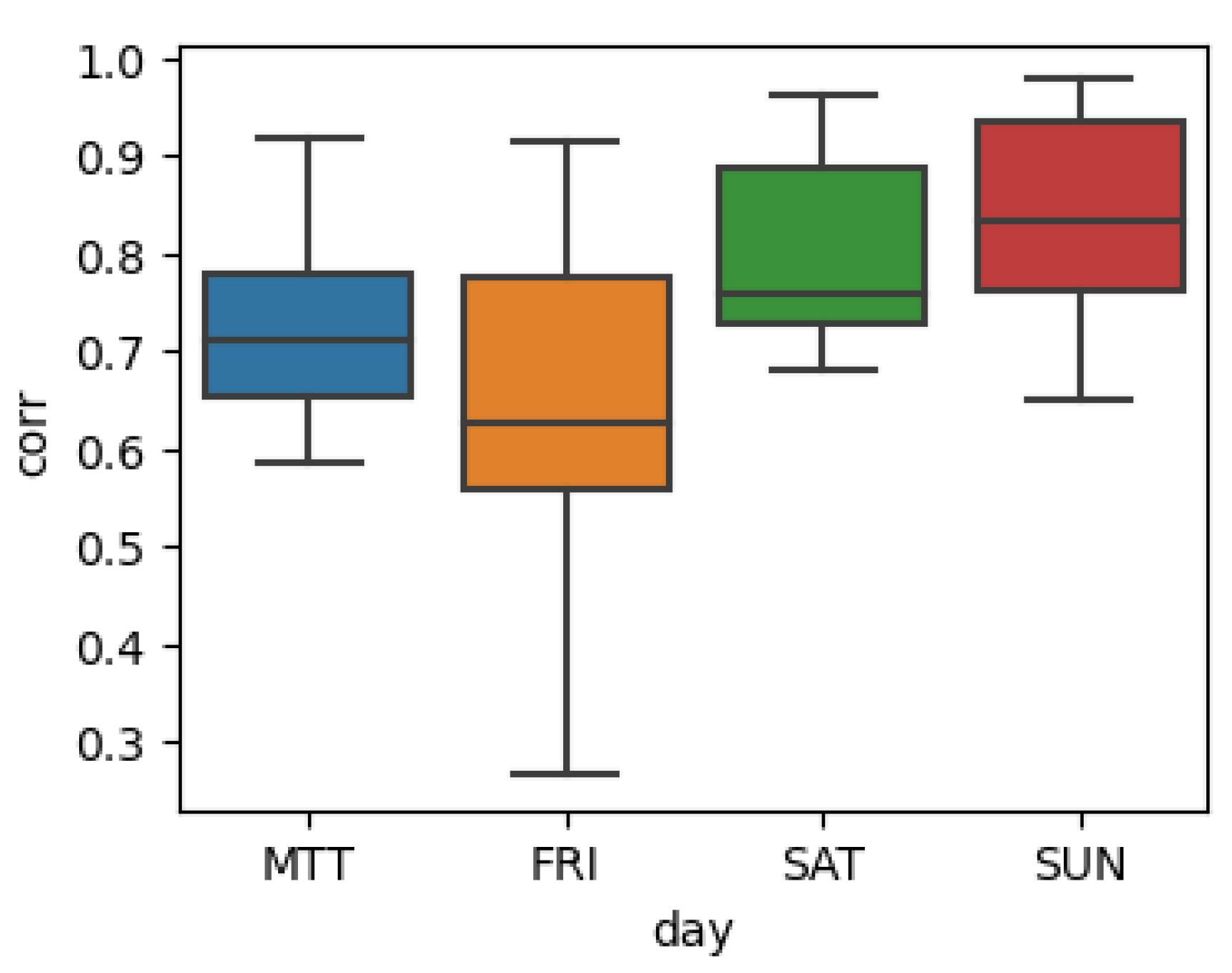
Figure A3.
Hourly footfall distribution of location 982, passenger flow and Google popular times of nearby Piccadilly Circus Station.
Figure A3.
Hourly footfall distribution of location 982, passenger flow and Google popular times of nearby Piccadilly Circus Station.
Appendix B. Case of Study
Appendix Case Study
Location 639, at 163 High Street, Greater London, is our case study to identify the best prediction method.
Figure A4.
Footfall time series of location 639.
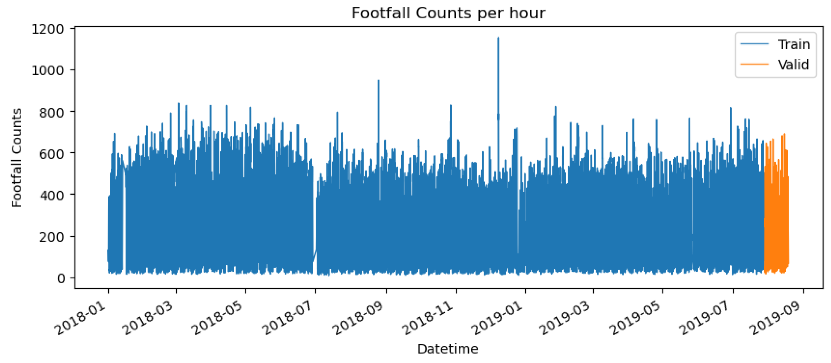
Figure A5.
Decompose of footfall time series by daily mean of location 639.
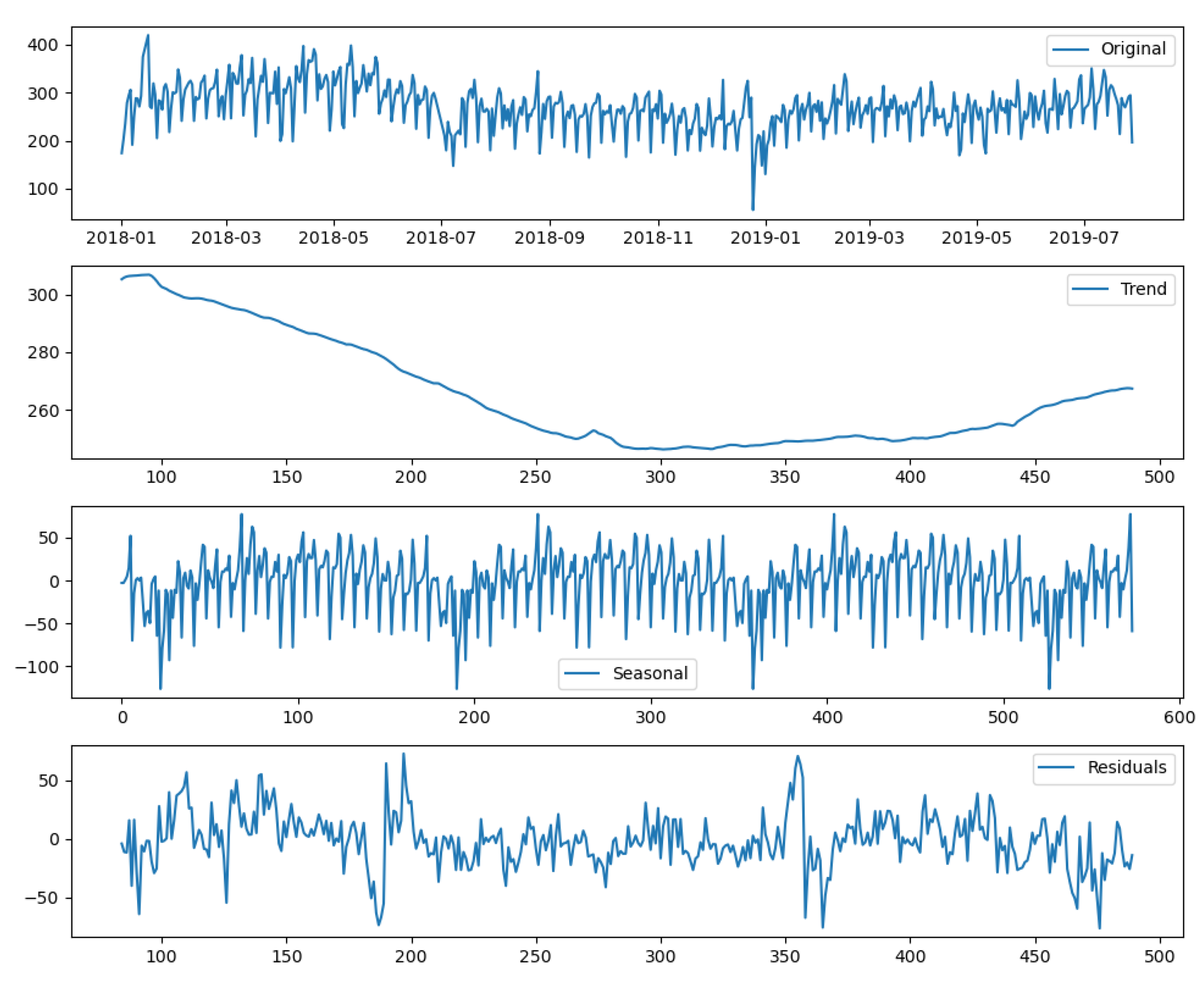
To estimate the parameters in HW and SARIMA models. For example, Figure A5 shows the components of footfall time series by daily mean. It can be seen from the seasonal component that in addition to week, there is also a complex periodicity for around half a year.
Figure A6.
Stationary test on footfall time series by daily mean of location 639.
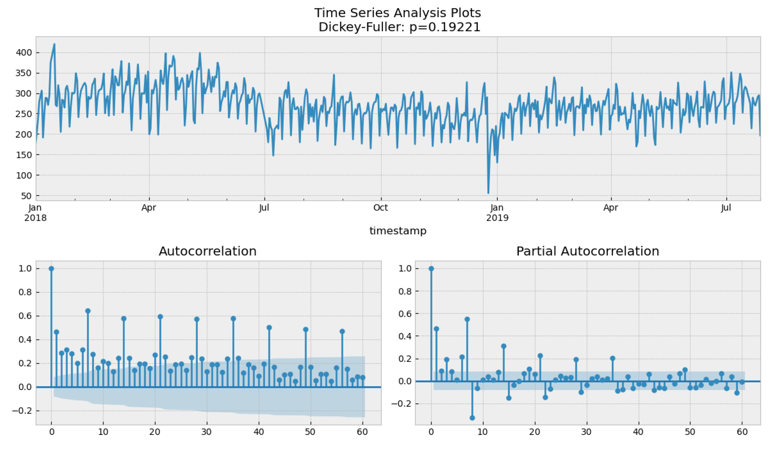
Figure A6 illustrates that the initial time series are non-stationary; the Dickey-Fuller test accepted the null hypothesis that a unit root is present. Figure 10 shows a visible fluctuation in the trend component. Therefore, the mean is not constant, and the variance is not stable throughout the series, indicating differentiation is needed in estimating the parameters of the SARIMA model.
The procedure of Auto-SARIMA indicates the SARIMA model with parameters (5, 1, 0) and (5, 1, 0) 7 has the lowest AIC, BIC and HQIC and shows a smaller RMSE than other parameter selections in empirical studies, indicating that these parameters are suitable for model fitting as well as prediction.
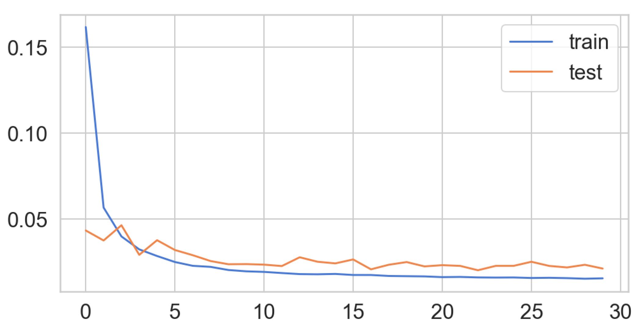
Figure A7 shows the train and test loss of the LSTM model. Results indicate that after 30 iterations, the loss curve drops to a stable stage and could be implemented to fit the time series.
Figure A7.
Train and test loss of LSTM of location 639.
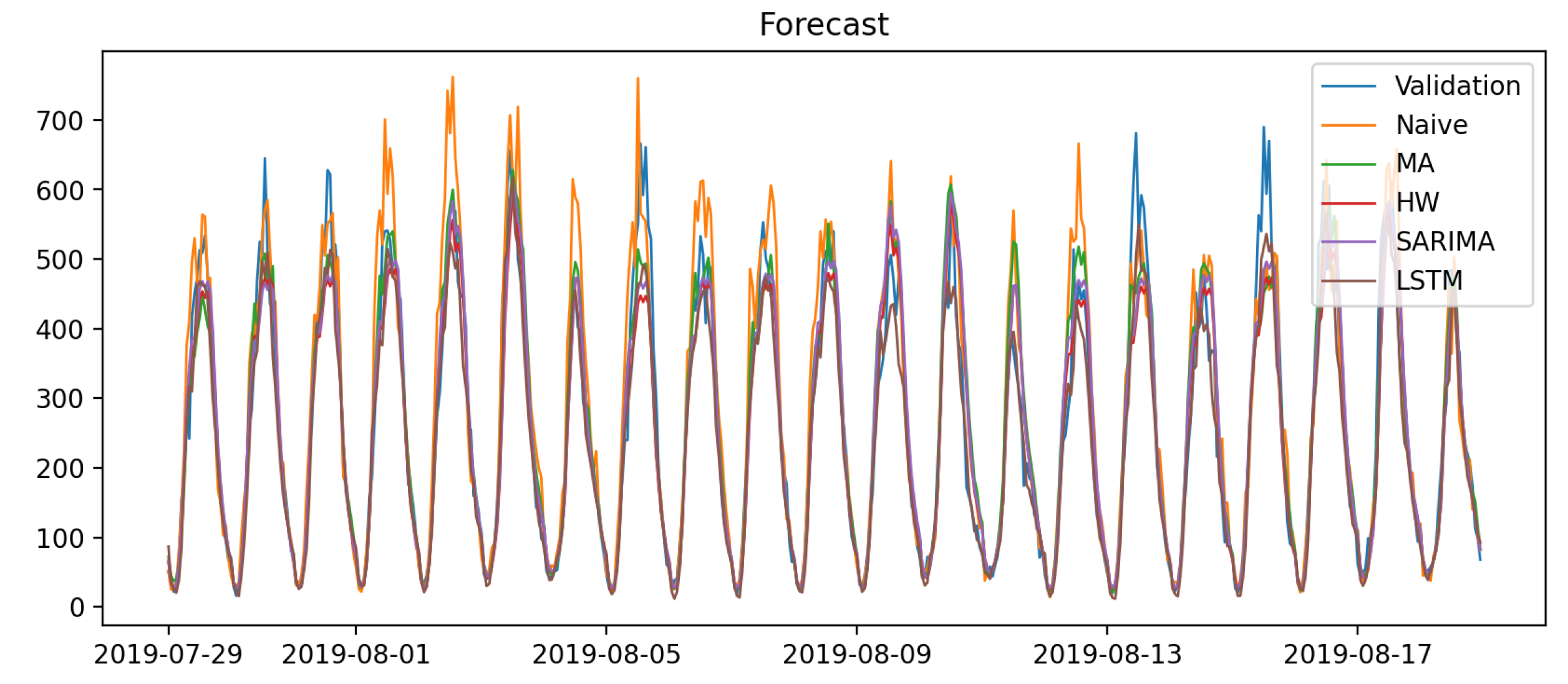
Results demonstrate that LSTM outperforms other models and becomes the optimal footfall prediction method in location 639 with a statistical significance.
Figure A8.
Forecasts on the test set—location 639.
References
- Waddington, T.; Clarke, G.; Clarke, M.C.; Hood, N.; Newing, A. Accounting for temporal demand variations in retail location models. Geographical Analysis 2019, 51, 426–447.
- Brown, S. Retail location theory: evolution and evaluation. International Review of Retail, Distribution and Consumer Research 1993, 3, 185–229.
- Lugomer, K.; Longley, P. Towards a comprehensive temporal classification of footfall patterns in the cities of Great Britain. In Proceedings of the Leibniz International Proceedings in Informatics, LIPIcs. Schloss Dagstuhl–Leibniz-Zentrum fuer Informatik, 2018, Vol. 114, p. 43.
- of Housing Communities & Local Government, M., 2019.
- Parker, C.; Ntounis, N.; Millington, S.; Quin, S.; Castillo-Villar, F.R. Improving the vitality and viability of the UK High Street by 2020: Identifying priorities and a framework for action. Journal of Place Management and Development 2017, 10, 310–348.
- Chapados, N.; Joliveau, M.; L’Ecuyer, P.; Rousseau, L.M. Retail store scheduling for profit. European Journal of Operational Research 2014, 239, 609–624.
- H, G., 2015.
- Zhang, P.; Li, X.Y.; Deng, H.Y.; Lin, Z.Y.; Zhang, X.N.; Wong, S.C. Potential field cellular automata model for overcrowded pedestrian flow. Transportmetrica A: Transport Science 2020, 16, 749–775. [CrossRef]
- Liu, M.; Li, L.; Li, Q.; Bai, Y.; Hu, C. Pedestrian flow prediction in open public places using graph convolutional network. ISPRS International Journal of Geo-Information 2021, 10, 455. [CrossRef]
- De Gooijer, J.G.; Hyndman, R.J. 25 years of time series forecasting. International journal of forecasting 2006, 22, 443–473.
- Sapankevych, N.I.; Sankar, R. Time series prediction using support vector machines: a survey. IEEE computational intelligence magazine 2009, 4, 24–38.
- Parmezan, A.R.S.; Batista, G.E. A study of the use of complexity measures in the similarity search process adopted by kNN algorithm for time series prediction. 2015 IEEE 14th International Conference on Machine Learning and Applications, ICMLA 2015 2016, pp. 45–51. [CrossRef]
- Cortez, P. Sensitivity analysis for time lag selection to forecast seasonal time series using neural networks and support vector machines. Proceedings of the International Joint Conference on Neural Networks 2010. [CrossRef]
- Kandananond, K. A comparison of various forecasting methods for autocorrelated time series. International Journal of Engineering Business Management 2012, 4, 1–6. [CrossRef]
- Ristanoski, G.; Liu, W.; Bailey, J. A time-dependent enhanced support vector machine for time series regression. Proceedings of the ACM SIGKDD International Conference on Knowledge Discovery and Data Mining 2013, Part F1288, 946–954. [CrossRef]
- Zhang, X.; Zhang, T.; Young, A.A.; Li, X. Applications and comparisons of four time series models in epidemiological surveillance data. PLoS ONE 2014, 9, e88075. [CrossRef]
- Parmezan, A.R.S.; Souza, V.M.; Batista, G.E. Evaluation of statistical and machine learning models for time series prediction: Identifying the state-of-the-art and the best conditions for the use of each model. Information Sciences 2019, 484, 302–337. [CrossRef]
- Gautam, A.; Singh, V. Parametric versus non-parametric time series forecasting methods: A review. Journal of Engineering Science and Technology Review 2020, 13, 165–171. [CrossRef]
- Weldegebriel, H.T.; Liu, H.; Haq, A.U.; Bugingo, E.; Zhang, D. A New Hybrid Convolutional Neural Network and eXtreme Gradient Boosting Classifier for Recognizing Handwritten Ethiopian Characters. IEEE Access 2020, 8, 17804–17818. [CrossRef]
- Guy, C. Retail location analysis. In Applied Geography; Routledge, 2002; pp. 450–462.
- Wang, W.; Wang, L.; Wang, X.; Wang, Y. Geographical Determinants of Regional Retail Sales: Evidence from 12,500 Retail Shops in Qiannan County, China. ISPRS International Journal of Geo-Information 2022, 11, 302.
- Consumer Data Research Centre SmartStreetSensor project. https://data.cdrc.ac.uk/dataset/local-data-company-ucl-smartstreetsensor-footfall-data-research-aggregated-data. Accessed: 01-06-2024.
- Soundararaj, B.; Cheshire, J.; Longley, P. Estimating real-time high-street footfall from Wi-Fi probe requests. International Journal of Geographical Information Science 2020, 34, 325–343.
- Murcio, R.; Soundararaj, B.; Lugomer, K. Movements in Cities: footfall and its spatio-temporal distribution. Consumer data research 2018, pp. 84–95.
- Trasberg, T.; Soundararaj, B.; Cheshire, J. Using Wi-Fi probe requests from mobile phones to quantify the impact of pedestrian flows on retail turnover. Computers, Environment and Urban Systems 2021, 87, 101601.
- Soundararaj, B. Estimating Footfall From Passive Wi-Fi Signals: Case Study with Smart Street Sensor Project. PhD thesis, UCL (University College London), 2019.
- TFL London Underground passenger counts data. https://api-portal.tfl.gov.uk/docs. Accessed: 2019-06-12. A valid API Key is needed to access the data.
- Box, G.E.; Jenkins, G.M.; Reinsel, G.C.; Ljung, G.M. Time series analysis: forecasting and control; John Wiley & Sons, 2015.
- Wei, W.W. Multivariate time series analysis and applications; John Wiley & Sons, 2019.
- Utlaut, T.L. Introduction to Time Series Analysis and Forecasting; Vol. 40, Hoboken, N.J. : Wiley-Interscience, 2008; pp. 476–478. [CrossRef]
- Sezer, O.B.; Gudelek, M.U.; Ozbayoglu, A.M. Financial time series forecasting with deep learning: A systematic literature review: 2005–2019. Applied Soft Computing Journal 2020, 90, 106181. [CrossRef]
- Ball, R.; Bartov, E. How naive is the stock market’s use of earnings information? Journal of Accounting and Economics 1996, 21, 319–337. [CrossRef]
- Hyndman, R. Forecasting: principles and practice; OTexts, 2018.
- Winters, P.R. Forecasting Sales by Exponentially Weighted Moving Averages. Management Science 1960, 6, 324–342. [CrossRef]
- Holt, C.C. Forecasting seasonals and trends by exponentially weighted moving averages. International Journal of Forecasting 2004, 20, 5–10. [CrossRef]
- Geurts, M.; Box, G.E.P.; Jenkins, G.M. Time Series Analysis: Forecasting and Control, rev. ed ed.; Vol. 14, San Francisco ; London : Holden-Day: San Francisco, 1977; p. 269. [CrossRef]
- Cristianini, N.; Shawe-Taylor, J. An introduction to support vector machines and other kernel-based learning methods; Cambridge university press, 2000.
- Cooper. A Bayesian Method for the Induction of Probabilistic Networks from Data. Machine Learning 1992, 9, 309–347. [CrossRef]
- Rasmussen, C.E. Gaussian processes in machine learning. In Summer school on machine learning; Springer, 2003; pp. 63–71.
- Hochreiter, S.; Schmidhuber, J. Long Short-Term Memory. Neural Computation 1997, 9, 1735–1780. [CrossRef]
- Graves, A.; Jaitly, N.; Mohamed, A.R. Hybrid speech recognition with Deep Bidirectional LSTM. 2013 IEEE Workshop on Automatic Speech Recognition and Understanding, ASRU 2013 - Proceedings 2013, pp. 273–278. [CrossRef]
- Greff, K.; Srivastava, R.K.; Koutnik, J.; Steunebrink, B.R.; Schmidhuber, J. LSTM: A Search Space Odyssey. IEEE Transactions on Neural Networks and Learning Systems 2017, 28, 2222–2232. [CrossRef]
- Zhang, L.; Zhang, L.; Du, B. Deep learning for remote sensing data: A technical tutorial on the state of the art. IEEE Geoscience and Remote Sensing Magazine 2016, 4, 22–40. [CrossRef]
- Fu, R.; Zhang, Z.; Li, L. Using LSTM and GRU neural network methods for traffic flow prediction. In Proceedings of the 2016 31st Youth academic annual conference of Chinese association of automation (YAC). IEEE, 2016, pp. 324–328.
- Diebold, F.X.; Mariano, R.S. Comparing predictive accuracy. Journal of Business & economic statistics 2002, 20, 134–144.
- Chen, W.; Zhang, S.; Li, R.; Shahabi, H. Performance evaluation of the GIS-based data mining techniques of best-first decision tree, random forest, and naïve Bayes tree for landslide susceptibility modeling. Science of the Total Environment 2018, 644, 1006–1018. [CrossRef]
- Taalab, K.; Cheng, T.; Zhang, Y. Mapping landslide susceptibility and types using Random Forest. Big Earth Data 2018, 2, 159–178. [CrossRef]
- Chikkakrishna, N.K.; Hardik, C.; Deepika, K.; Sparsha, N. Short-term traffic prediction using sarima and FbPROPHET. 2019 IEEE 16th India Council International Conference, INDICON 2019 - Symposium Proceedings 2019. [CrossRef]
- Chen, T.; Guestrin, C. XGBoost: A scalable tree boosting system. Proceedings of the 22nd ACM SIGKDD International Conference on Knowledge Discovery and Data Mining 2016, pp. 785–794.
Figure 1.
Proposed workflow to select the optimal footfall forecasting algorithm. Footfall derived from Wi-Fi signals.
Figure 1.
Proposed workflow to select the optimal footfall forecasting algorithm. Footfall derived from Wi-Fi signals.
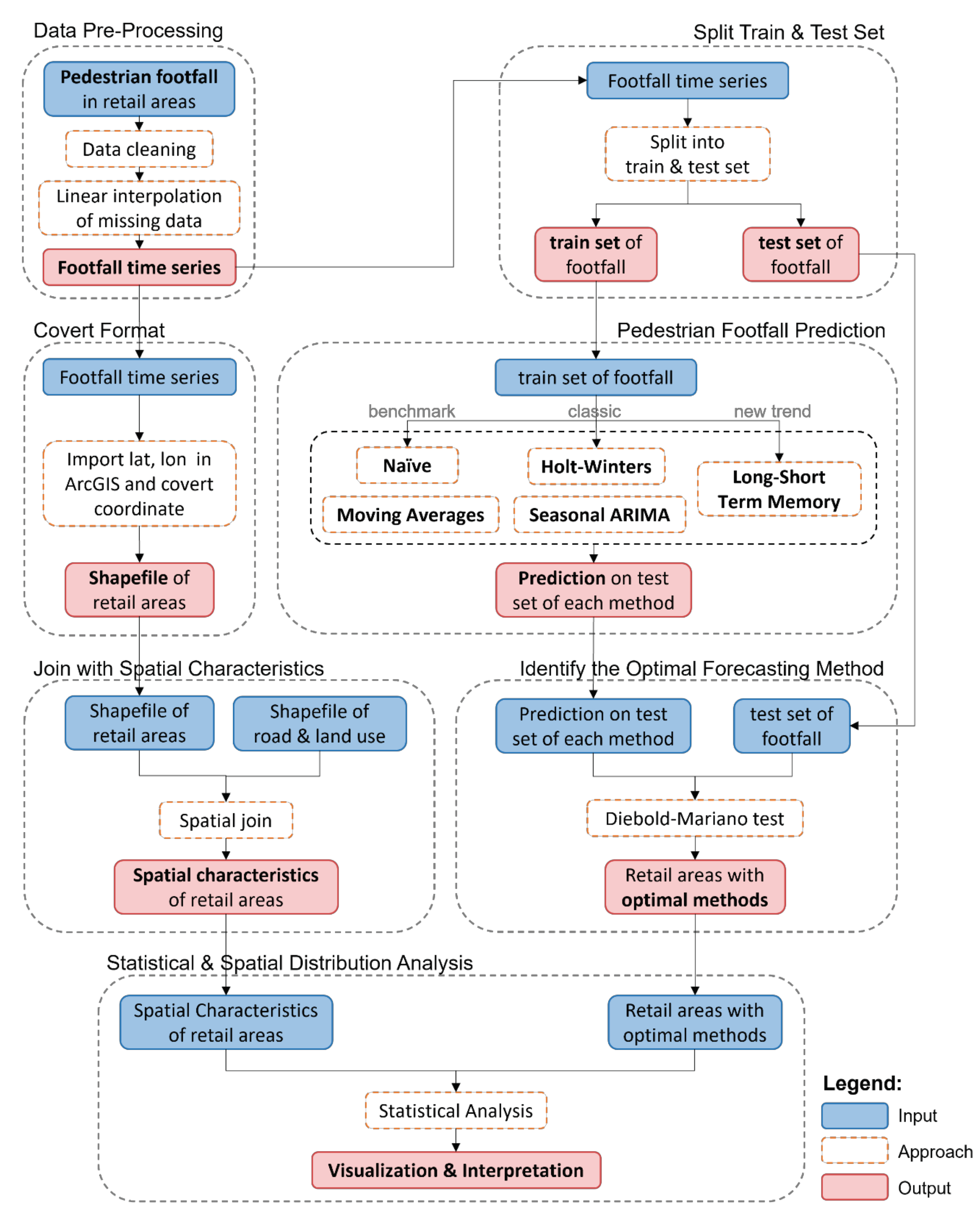
Figure 2.
Spatial distribution of Wi-Fi sensors in Great Britain.
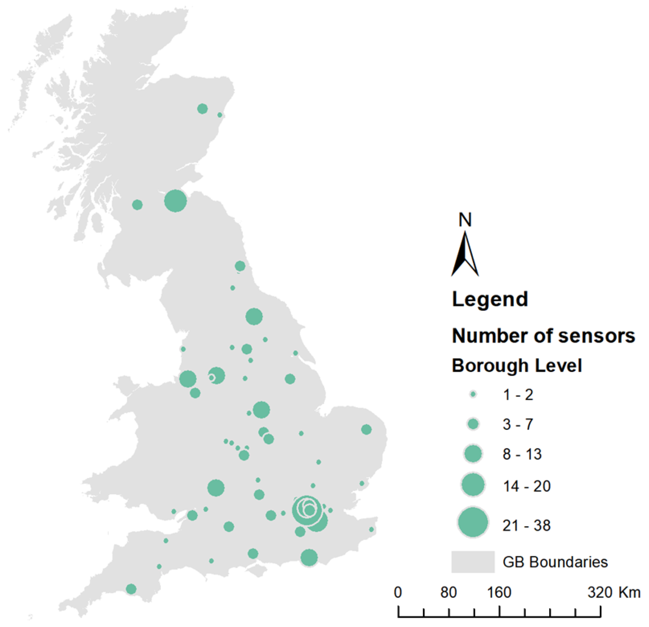
Figure 3.
Average footfall counts every 5 minutes in GB retail areas.
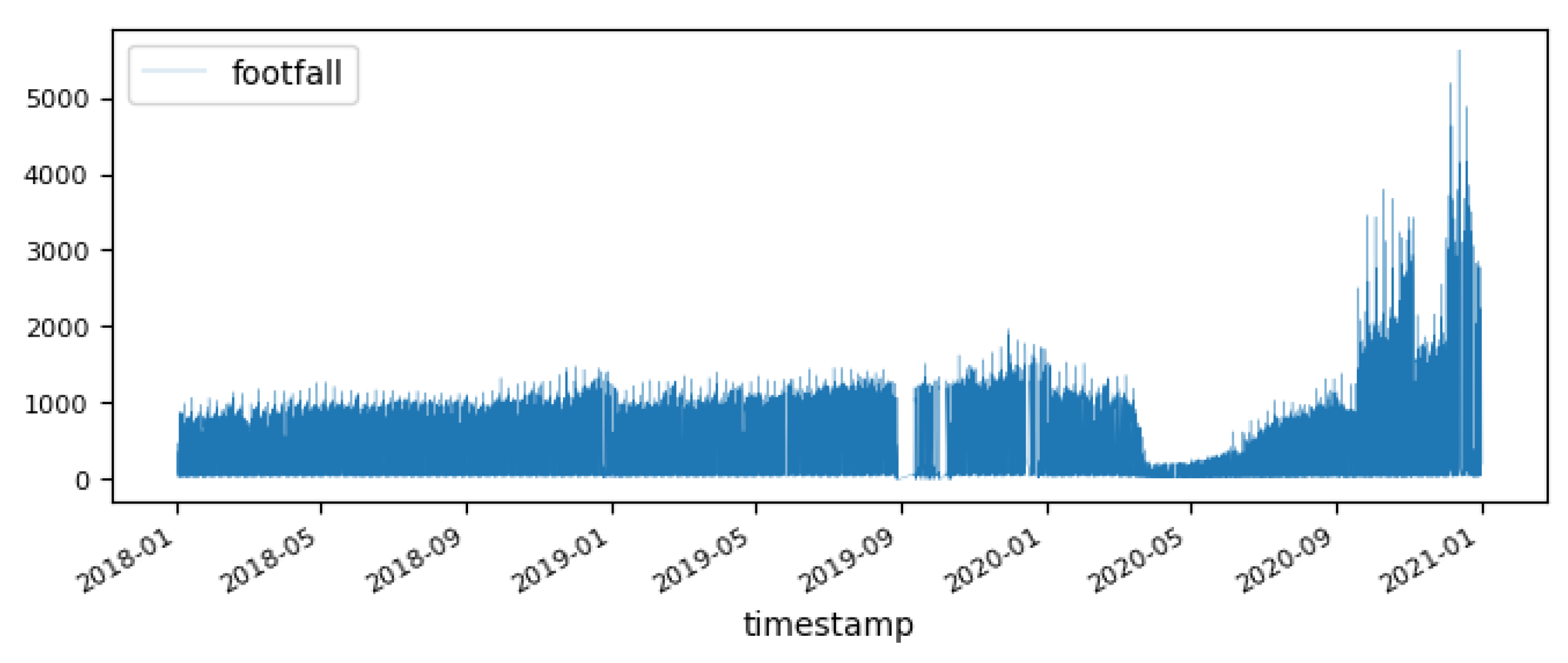
Figure 6.
Hourly footfall distribution of location 709.
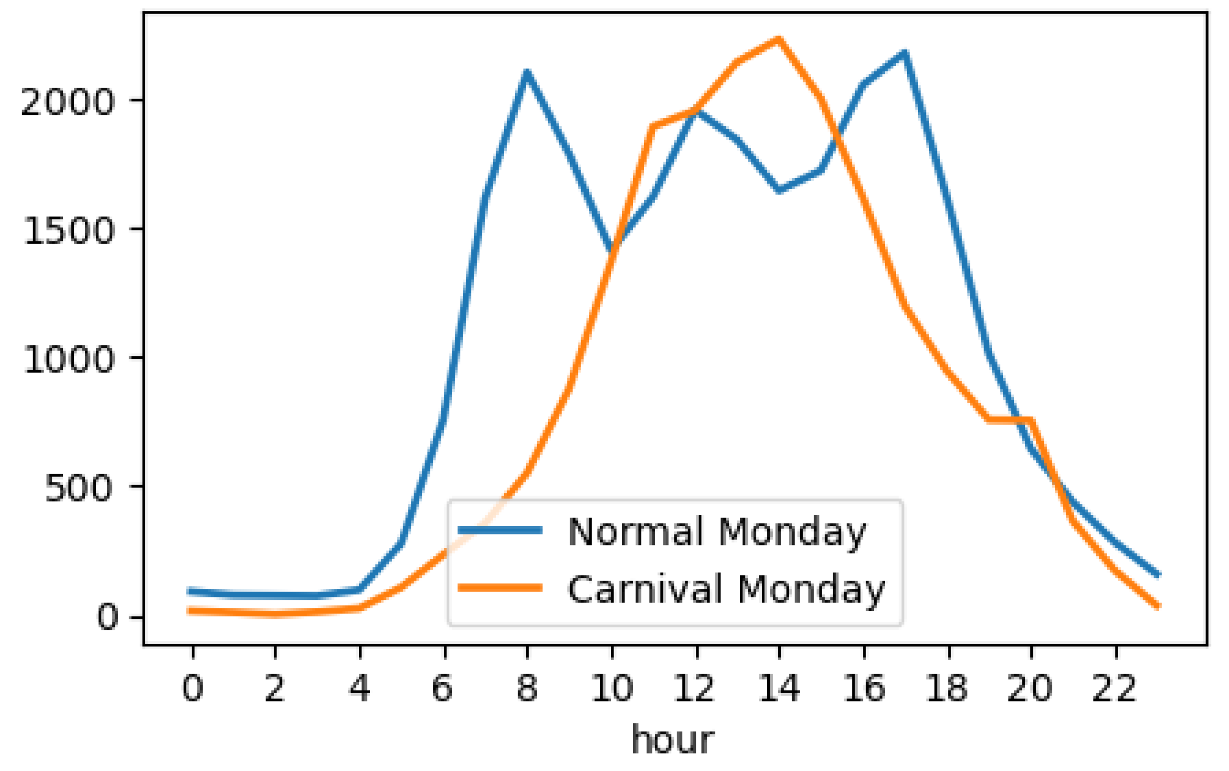
Figure 7.
Pearson correlation between FF in retail areas and nearby underground flows on different days of the week. The label MTT represents Monday to Thursday measures.
Figure 7.
Pearson correlation between FF in retail areas and nearby underground flows on different days of the week. The label MTT represents Monday to Thursday measures.
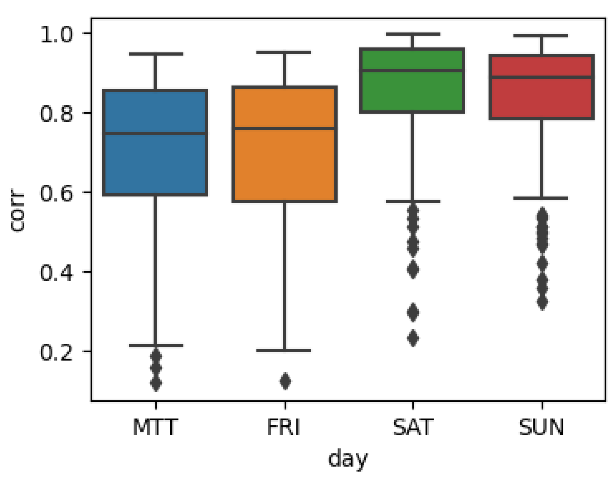
Figure 8.
Footfall prediction results. (a) Optimal method counts. (b) Statistics of average missing data ratio.
Figure 8.
Footfall prediction results. (a) Optimal method counts. (b) Statistics of average missing data ratio.
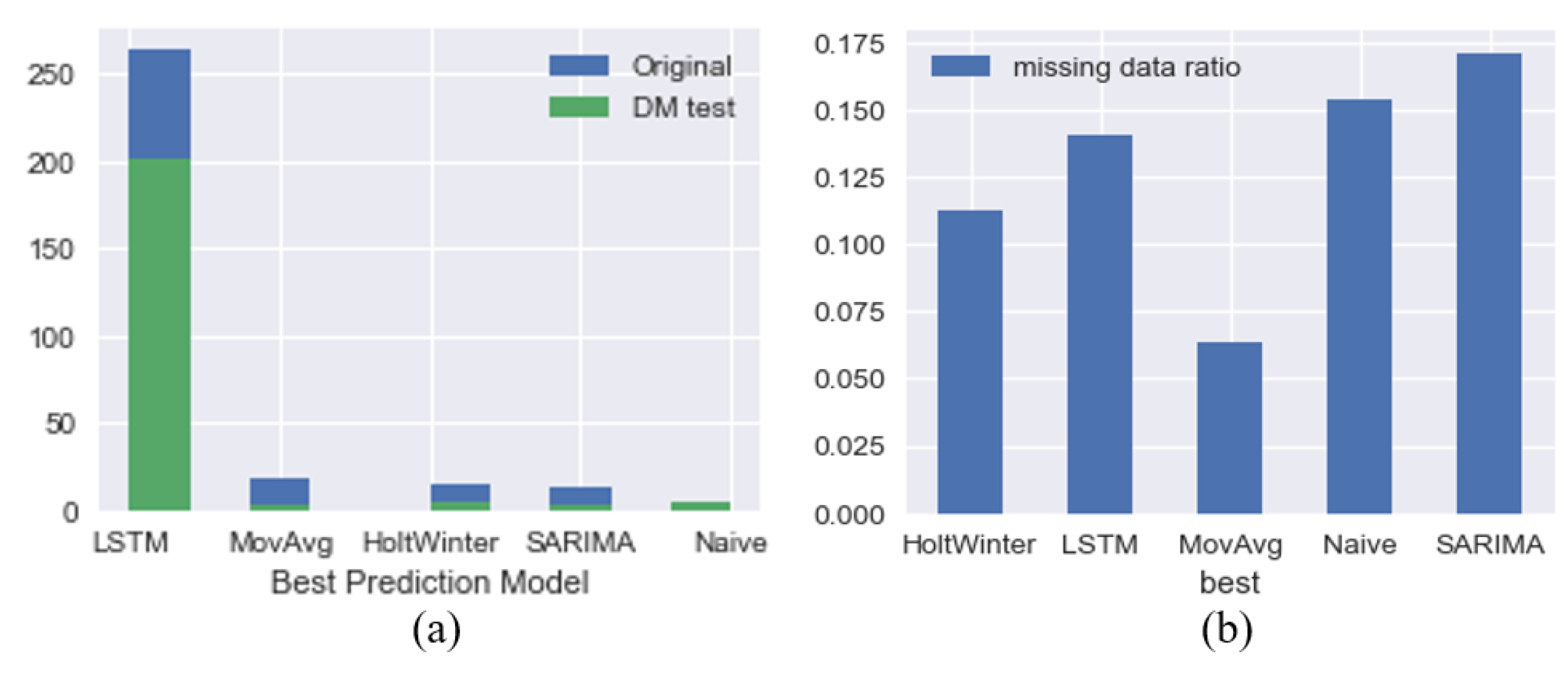
Figure 9.
Footfall prediction results. (a) Optimal method counts, (b) Statistics of average missing data ratio (without LSTM).
Figure 9.
Footfall prediction results. (a) Optimal method counts, (b) Statistics of average missing data ratio (without LSTM).
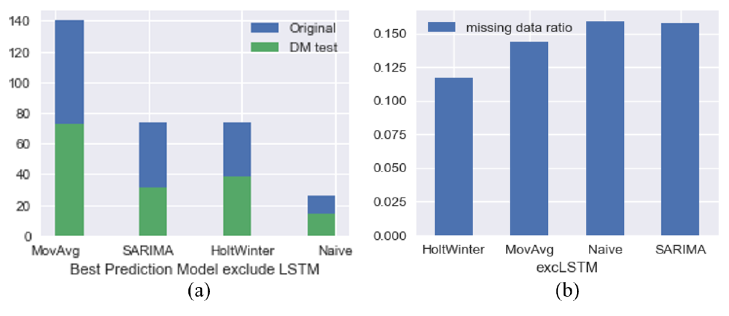
Figure 10.
Average footfall distribution of locations with different optimal methods. by (a) Hour. (b) Day of the week. (c) Month.
Figure 10.
Average footfall distribution of locations with different optimal methods. by (a) Hour. (b) Day of the week. (c) Month.
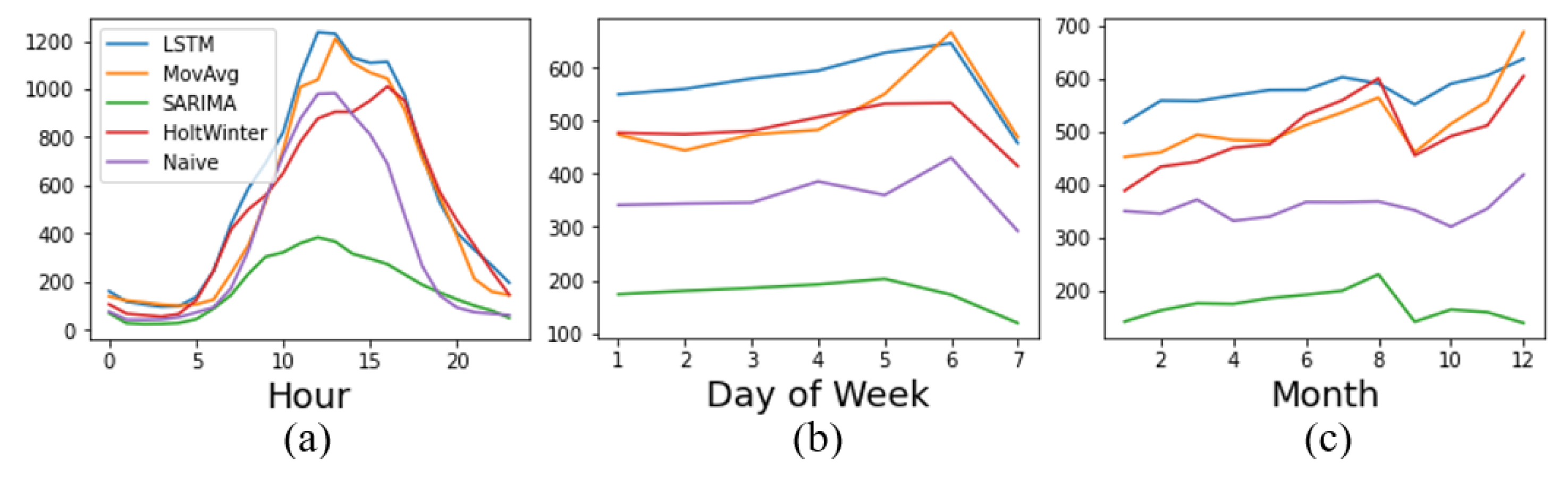
Figure 11.
Average distance from different locations to roads.
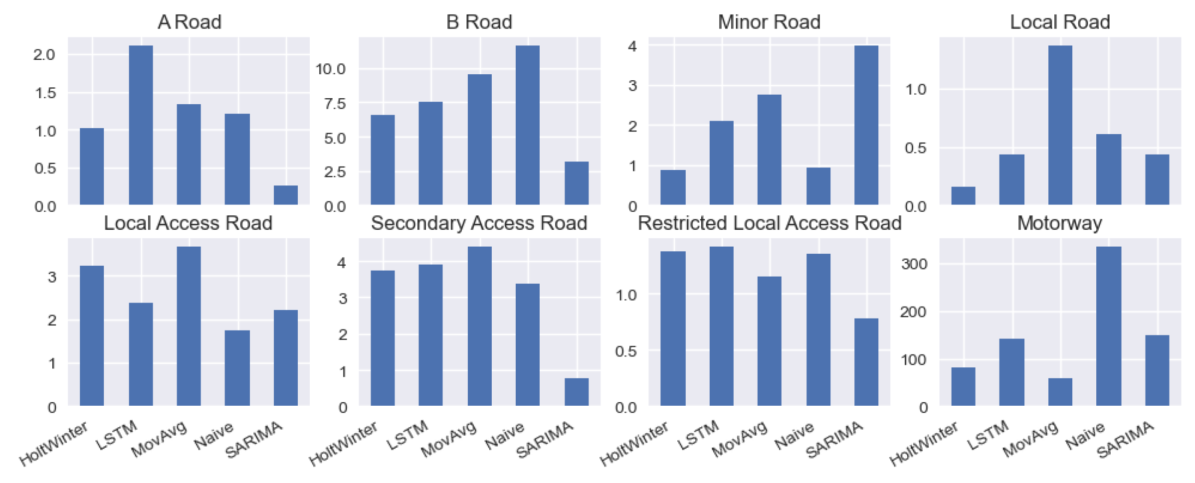
Figure 12.
Land classification statistics on locations with different optimal prediction methods.
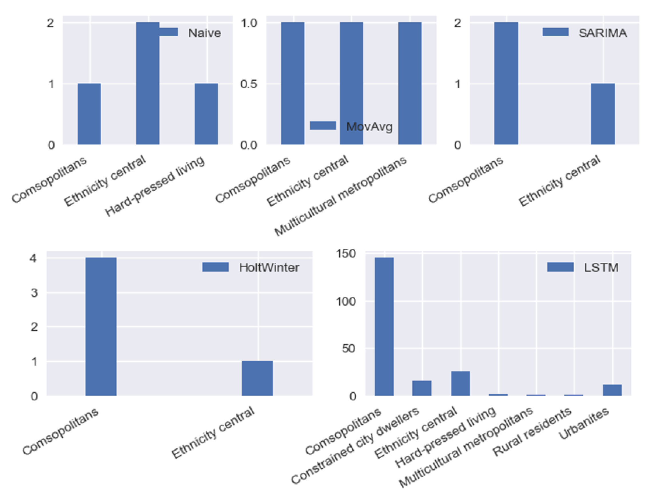
Figure 13.
Correlation matrix of continuous variables.
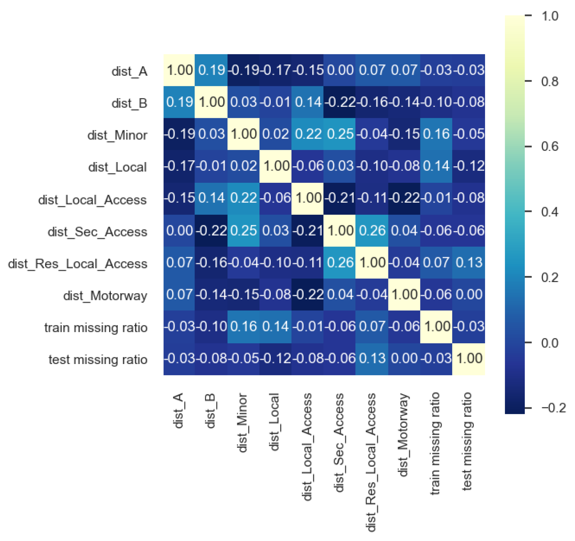
Figure 14.
Importance of top 10 variables.
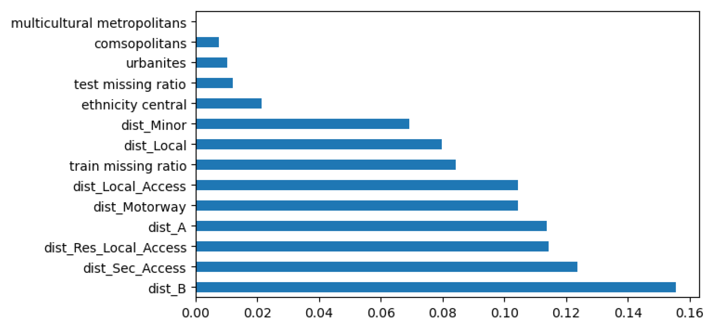

Table 1.
Performance of different time series prediction models.
| Best Method | Significance | ||||
|---|---|---|---|---|---|
| Method | RMSE | Counts | % | Counts | % |
| 254.24 | 5 | 1.59% | 4 | 1.84% | |
| 216.68 | 18 | 5.73% | 3 | 1.38% | |
| 254.24 | 15 | 4.78% | 5 | 2.30% | |
| 221.61 | 13 | 4.14% | 3 | 1.38% | |
| 224.67 | 263 | 83.76% | 202 | 93.10% | |
| NA | 314 | 100.00% | 217 | 100.00% | |
Table 2.
Performance of different time series prediction models.
| Best Method | Significance | ||||
|---|---|---|---|---|---|
| Method | RMSE | Counts | % | Counts | % |
| 254.24 | 26 | 8.28% | 14 | 1.27% | |
| 216.68 | 140 | 44.59% | 73 | 0.96% | |
| 221.61 | 74 | 23.57% | 39 | 1.59% | |
| 224.67 | 74 | 23.57% | 31 | 0.96% | |
| NA | 314 | 100.00% | 157 | 100.00% | |
Disclaimer/Publisher’s Note: The statements, opinions and data contained in all publications are solely those of the individual author(s) and contributor(s) and not of MDPI and/or the editor(s). MDPI and/or the editor(s) disclaim responsibility for any injury to people or property resulting from any ideas, methods, instructions or products referred to in the content. |
© 2024 by the authors. Licensee MDPI, Basel, Switzerland. This article is an open access article distributed under the terms and conditions of the Creative Commons Attribution (CC BY) license (http://creativecommons.org/licenses/by/4.0/).
Copyright: This open access article is published under a Creative Commons CC BY 4.0 license, which permit the free download, distribution, and reuse, provided that the author and preprint are cited in any reuse.


