

Submitted:
03 December 2024
Posted:
06 December 2024
You are already at the latest version
Abstract
We propose a method – based on a filtered Markov process – to convert 10–min rain–rate time series into 1–min time series – i.e. quasi instantaneous rainfall – the latter to be used as input to the Synthetic Storm Technique – a very reliable tool – for calculating rain–attenuation time series in satellite communication systems, or to estimate runoff, erosion, pollutant transport and other applications in hydrology. To develop the method, we use a very large data bank of 1–min rain–rate time series collected in several sites with different climatic cnditions. We first convert them into 10–min rain–rate time series – to obtain the measured data provided by some Meteorological Institutes – then, from this latter data, we develop the method that generates 1–min rain–rate time series and compare them with the measured ones. The two time series agree very well. Afterwards, we use them to simulate rain attenuation time series at 20.7 GHz, in 35.5° slant paths to geostationary satellites. The two simulated rain attenuation probability distributions show very small differences, therefore we conclude that the rain–rate conversion method is very reliable.
Keywords:
Instantaneous rainfall
; filtered Markov process
; meteorology
; rain attenuation
; satellite communication
; rain rate conversion
; rain–rate time series
1. Introduction
The purpose of this paper is to develop and propose a method to convert 10–min rain–rate time series into 1–min rain–rate time series, the latter to be afterwards used, in the paper, as input to the Synthetic Storm Technique (SST) for simulating rain–attenuation time series [1], a very reliable tool that can even reconstruct missing intervals in time series [2]. The rationale for the need of such a method lies in the fact that several meteorological institues make available time series of quantity of water accumulated every 10 minutes (therefore providing 10–min rain–rate time series), compared to the past when, at most, the quantity of water collected referred from 1 day to 1 hour. Our previous theory on the de–integration of the accumulated rainfall – from 1 day to 1 hour water – refers only to the probability distributions of rain–rate [3,4].
To develop the method, we use a very large data bank of 1–min rain–rate time series collected in Spino d’Adda (Table 1), from 1993 to 2002, 10 years of practically all rain events occurred in the period. First, we convert them to 10–min rain–rate time series for obtaining the measured data bank allegedly provided by some Meteorological Institutes, and then we develop the method that can simulate 1–min rain–rate time series. The comparison between the experimental and simulated 1–min time series will provide how good and precise the method is. The conversion method is then studied and developed for the other sites listed in Table 1, to assess whether it works well also in different climatic regions.
The sites listed in Table 1 are useful study–cases because: (a) on–site 1–min rain–rate time series were continuously recorded for several years; (b) in these sites are located important NASA and ESA satellite ground stations (Gera Lario, Fucino, Madrid, White Sands); (c) long–term radio propagation experiments were performed (Fucino, Gera Lario, Spino d’Adda, Madrid, Prague, White Sands); (d) there are important cities (Madrid, Prague, Tampa, Vancouver).
Afterwards, we use the two sets of 1–min rain–rate time series (i.e., that measured and that simulated from 10–min rain–rate time series) as the input to the SST for simulating – as example of application – rain attenuation time series at 20.7 GHz in 35.5° slant paths to geostationary satellites at the sites of Table 1. The conclusion of our exercise is that the two rain attenuation probability distributions in an average year show no significant differences that can affect satellite systems design at centimeter or millimeter frequencies, so that the method can be used very reliably for this purpose.
The theory, however, can be potentially useful not only in satellite communications and radio propagation studies, but also in other fields. In agriculture, for example, the measured daily rainfall needs to be disaggregated to predict runoff, erosion and pollutant transport [5,6,7,8]. In hydrology, the kinetic energy determines the potential ability of the rainfall to detach soil and it is used as a rain erosivity index [6]. Kinetic energy is strictly linked to the rain rate, therefore data of instantaneous rain rate (as 1–min rain rate times series can be considered) could improve the estimates in these fields.
After this introductory section, in Section 2 we study the 1–min and 10–min rain–rate data bank of Spino d’Adda, our “laboratory” site; in Section 3 we develop the method to convert into 1-min rain rate time series, termed in Spino d’Adda; in Section 4 we develop and confirm the method for the other sites of Table 1; in Section 5 we recall the theory of the Synthetic Storm Technique and report its application to the sites of Table 1; in Section 6 we draw a conclusion.
2. Exploratory Data Analysis in Spino d’Adda
In this Section we use the 10–year 1–min rain rate data bank collected in Spino d’Adda, our “laboratoty” site, to study how the experimental 1–min rain–rate time series (mm/h) are connected with the corresponding 10–min time series (mm/h). The latter is generated by , according to the following relationhsip, applied to disjoint and contiguous 10–min intervals during the rainfall event:
Figure 1 shows an example of this linear tranformation. We notice, of course, that is smoothed, therefore any application using will underestimate the effect of the “instantaneous” largest rain rates whose intensity can be significantly reduced.
Since we transform (mm/h) into an estimated/simulated , the first step is to study the distribution of within intervals of 10 min conditioned to . These conditional distribution will be useful to simulate from . This is possible because, as shown in the example of Figure 1, both , and are available for Spino d’Adda and the other sites listed in Table 1, for several years. By considering the full data bank of similar results, we have therefore calculated the conditional histograms of within 10–min intervals, in the following ranges of : 0–2, 2–4, 4–6, 6–8, 8–10, 10–15, 15–20, 20–30, 30–40, > 40 mm/h (samples with range maximum value are included in that range). Notice that the first range starts at 0.2 mm/h because of rain–gauge technology. Figure 2, Figure 3, Figure 4, Figure 5 and Figure 6 show these histograms.
From these figures we assume that a log–normal probability density function (PDF) can adequately model the central part of the experimental histograms, therefore we have calculated mean value and standard deviation of – natural logarithm – and assumed a log–normal probability PDF chacterized by the values reported in Table 2, together with the correlation coefficient between two successive samples within the same 10–min interval. These parameters are fundamental because they will be used in Section 3 to simulate from .

Table 1.
Mean value, standard deviation of and correlation coefficient between two successive samples within the same 10–min interval, for the indicated ranges. The first range starts at 0.2 mm/h.
Table 1.
Mean value, standard deviation of and correlation coefficient between two successive samples within the same 10–min interval, for the indicated ranges. The first range starts at 0.2 mm/h.
| (mm/h) | Mean | Standard Deviation | Correlation Coefficient |
| 0–2 | –0.60 | 0.75 | 0.94 |
| 2–4 | 0.94 | 0.37 | 0.76 |
| 4–6 | 1.51 | 0.41 | 0.70 |
| 6–8 | 1.83 | 0.49 | 0.72 |
| 8–10 | 2.07 | 0.52 | 0.68 |
| 10–15 | 2.35 | 0.61 | 0.72 |
| 15–20 | 2.62 | 0.76 | 0.71 |
| 20–30 | 3.03 | 0.68 | 0.70 |
| 30–40 | 3.32 | 0.77 | 0.75 |
| > 40 | 3.95 | 0.72 | 0.76 |
3. From to
In this section we describe how to convert into the final 1-min rain rate series to . In Appendix A we report the list of mathematical symbols. First, we show how to get the first version of , termed simulated . First, we estimate the sample from the previous sample within a 10–min interval, then we filter to reduce the high–frequency noise introduced by the simulation. In all cases, the experimental quantity of water collected in each 10–min interval in conserved by using a suitable scaling factor.
3.1. Simulation Steps
Since any conditional PDF is modelled as log–normal within each 10–min interval, we model the bivariate probability density function between two succesive values and , in the 10–min interval, as log–normal – we think this modelling can adequately describe at least the central part of the bivariate probability density – therefore can be estimated from by considering the conditional log–normal PDF, as follows.
Since within the same 10–min rain rate range (see Table 2) and , Eqs.(2)(3) become:
Now, we can detail the simulation steps:
- Sample 1 of (t). According to the sample 1 of – in a real application this would be the first value of the provided by Meteorological Institutes – the mean value and the standard deviation of the conditional PDF and the correlation coefficient are selected from Table 1.
-
A standard Gaussian random number is generated and denormalized according to the values of step 1, according to the following relationships:For example, let mm/h and (randomly generated), then (from Table 2) , , , therefore mm/h.
- Samples 2 to 10. A standard Gaussian random number is generated for each sample as in step 2, but now it is denormalized according to Eqs (4)(5). Continuing the example of step 2: mm/h; let (randomly generated), then and , therefore mm/h. Since the next sample depends only the previous one, the simulation process is a first–order Markov process [12].
-
The 1–min rain–rate sample is scaled to conserve the quantity of water of the original sample, the latter given by:Now, the quantity of water in the simulation is given by:Since in general, , to conserve the quantity of water each 1–min sample must be scaled to obtain the rain–rate time series :
- The simulation process is repeated by considering the successve value , till the last sample of the rain event. The passage from sample 10 simulated from to the sample 1 of the next sample is memoryless, therefore step 1 is repeated without recalling sample 10 of the previous interval. Moreover, notice that we neglect the “border” distortion due to the last 10–min sample of in a rain event because this interval may not be completely rainy (an information lost, of course, also in real experimental data).
The 1–sample memory steps 1–4 and the memoryless step 5 simplify the simulation but introduce high frequency noise as shown in Figure 7. This noise can be reduced by digital filtering, as we show in the next sub–section.
3.2. Optimum Filter
To reduce the noise produced by the sumulation steps, is filtered with a low–pass Butterworth filter of order 10 [13,14] therefore producing . Also must be scaled to conserve the experimental quantity of water of the 10–min interval. In conclusion, by filtering and scaling we get the final 1–min rain–rate time series , according to:
With:
The only parameter which defines the transfer function of the filter is its cut–off frequency , where is the Nyquist frequency [13,14].
To determine the optimum value , we consider the error (mm/h) between the rain rate simulated and the rain rate measured at equal probabiltiy exceeded:
Figure 8 shows mean value and standard deviation of versus . It can be noted that: (a) the mean error is very small in the entire range ( mm/h); (b) the standard deviation is minimum at about , therefore, in the following we fix for all simulations.
Figure 9 show the same time series of Figure 7 after the full simulation process just described. Finally, Figure 10 shows the overall result of this exercise by drawing the probability distrbution (PD) that the 1–min rain rate in abscissa is exceeded in the experimental data, i.e. , and in the simulated 1–min data, . The two curves are almost indistinguishable, in agreement with the error and standard deviation reported in Figure 8 at .
4. From to in Other Sites
In this section we apply the method obtained in our “laboratory” of Spino d’Adda at the sites reported in Table 1, for which 1–min rate times series are available for many years. First, in Figure 11, we show the scatterplots between mean values, standard deviations and correlation cofficients of Spino d’Adda (the values of Table 2) versus those of the othe sites of Table 1 (Appendix B reports the numerical values). We can see a very tight relationship between the mean values. This means that the rain rate process, although in sites with different weather and rainfall intensity, can be modelled with log–normal PDFs with the same mean value. Differences arise in the standard deviation and correlation coefficient, although these differences do not impact significantly on the simulation predictions as we show next.
Figure 11.
Scatterplots of mean values (left panel), standard deviations (central panel) and correlation coefficients (right panel) between the values of the sites of Table 1 and Spino d’Adda. Gera Lario: green; Fucino: blue; Madrid: cyan; Prague: yellow; Tampa: red; White Sands: magenta; Vancouver: black.
Figure 11.
Scatterplots of mean values (left panel), standard deviations (central panel) and correlation coefficients (right panel) between the values of the sites of Table 1 and Spino d’Adda. Gera Lario: green; Fucino: blue; Madrid: cyan; Prague: yellow; Tampa: red; White Sands: magenta; Vancouver: black.
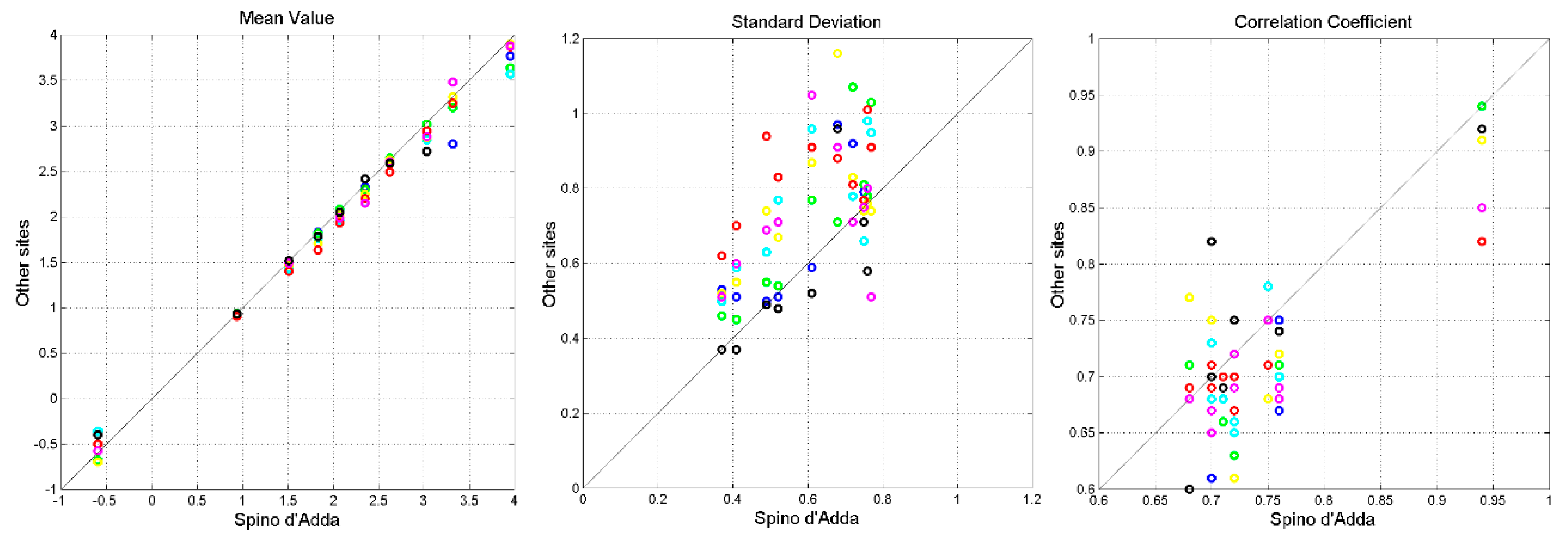
Figure 12.
Gera Lario. Probability distrbution that the 1–min rain rate in abscissa is exceeded in the experimental data, , blue line, and in the simulated 1–min data, , black line. Left panel: is obtained by using local values of the conditional PDFs; Right panel: is obtained by using Spino d’Adda conditional PDFs (Table 2).
Figure 12.
Gera Lario. Probability distrbution that the 1–min rain rate in abscissa is exceeded in the experimental data, , blue line, and in the simulated 1–min data, , black line. Left panel: is obtained by using local values of the conditional PDFs; Right panel: is obtained by using Spino d’Adda conditional PDFs (Table 2).
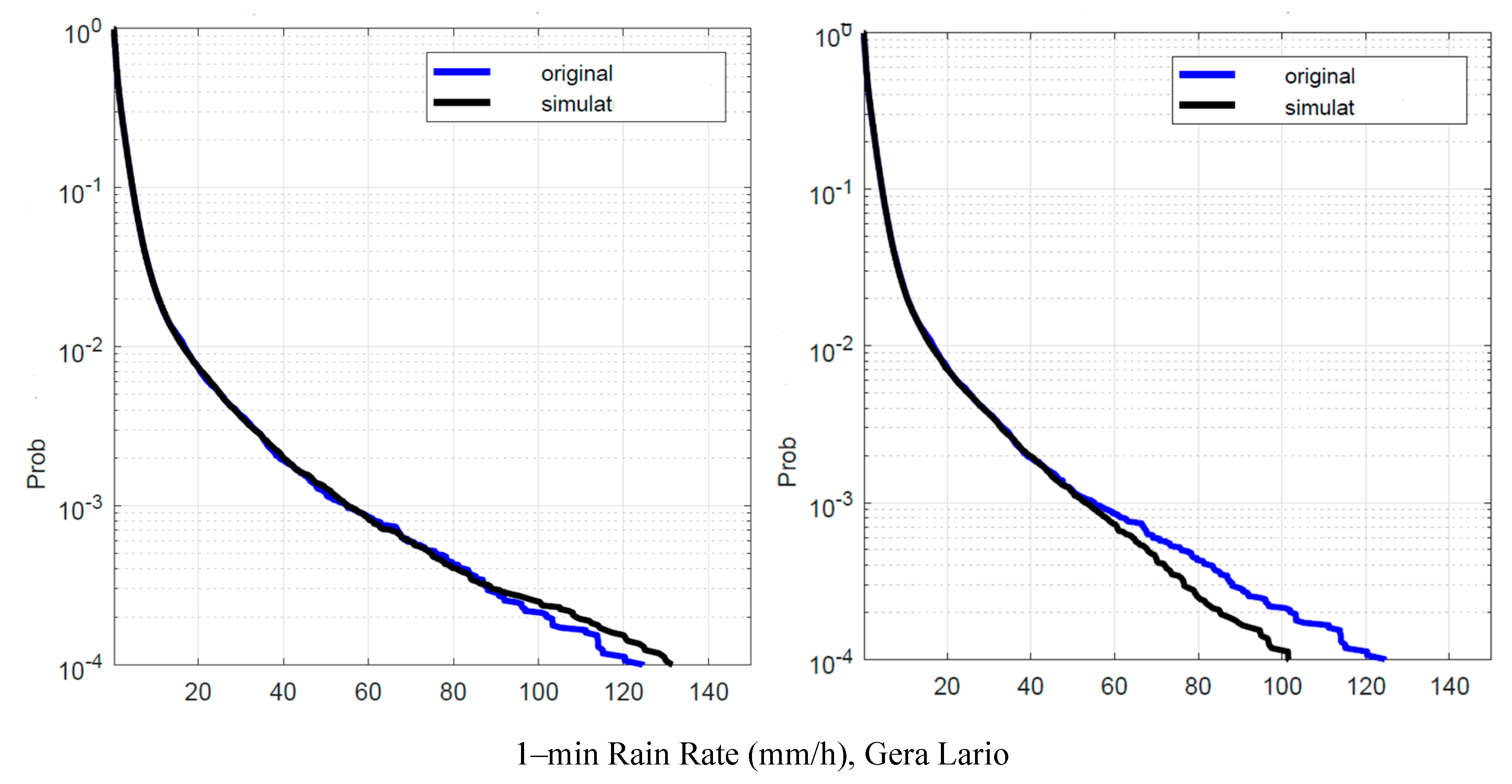
Figure 13.
Fucino. Probability distrbution that the 1–min rain rate in abscissa is exceeded in the experimental data, , blue line, and in the simulated 1–min data, , black line. Left panel: is obtained by using local values of the conditional PDFs; Right panel: is obtained by using Spino d’Adda conditional PDFs (Table 2).
Figure 13.
Fucino. Probability distrbution that the 1–min rain rate in abscissa is exceeded in the experimental data, , blue line, and in the simulated 1–min data, , black line. Left panel: is obtained by using local values of the conditional PDFs; Right panel: is obtained by using Spino d’Adda conditional PDFs (Table 2).
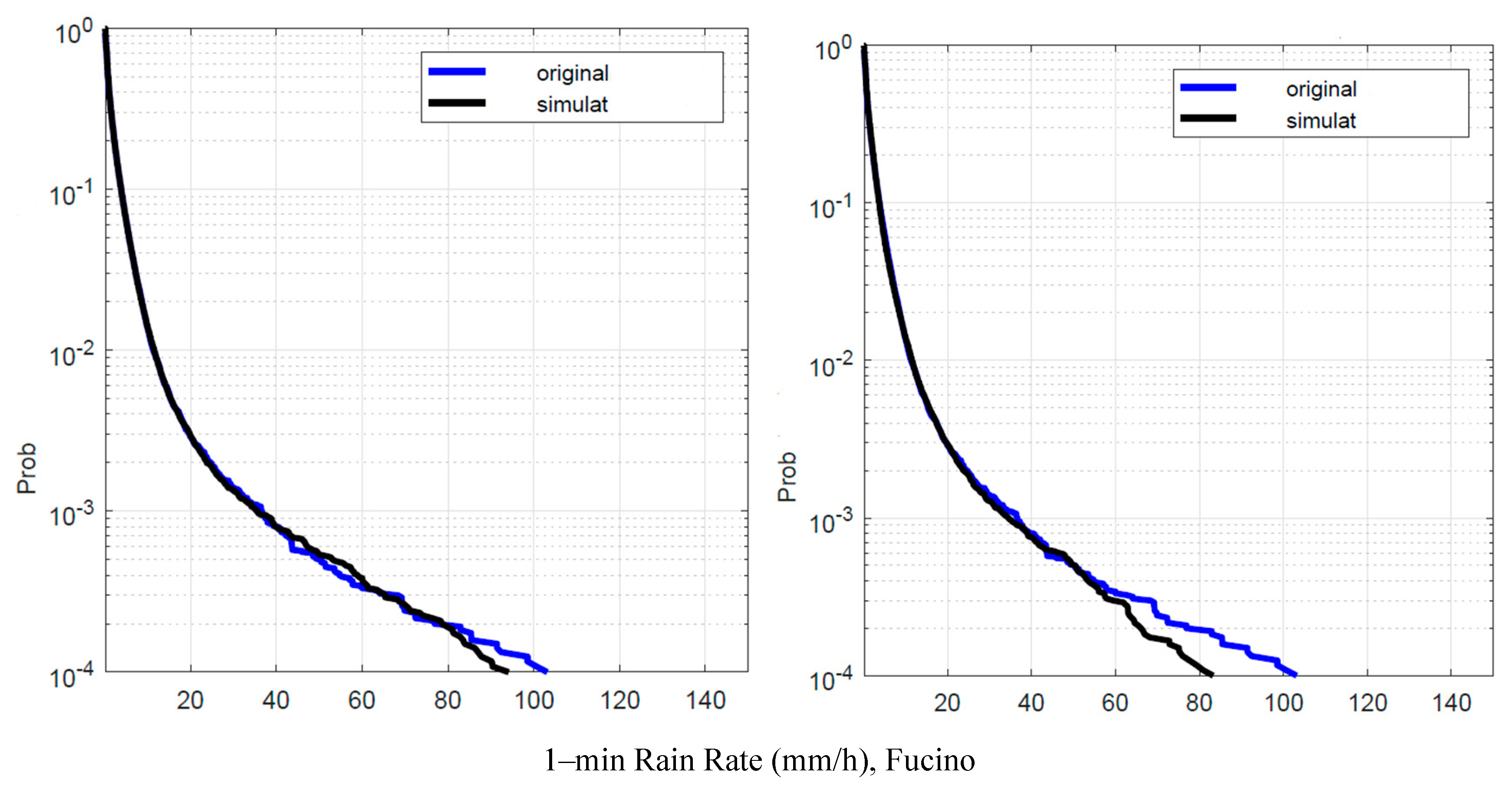
From these figures we notice that the simulation with the local conditional PDFs (Appendix B) gives better results than that with the parameters of Spino d’Adda (Table 2), as expected. However, notice that in the simulations with the data of Spino d’Adda, the largest errors mostly occur at the lowest probabilities. In real applications, as the one we show in the next sections, these probabilities correspond to few minutes. For example, in Madrid – Figure 14, the worst site for this comparison –, in the arithmetic average year of the 9–year period here considered, for about 2.2% of the time, i.e. about min. Now, Figure 14 shows that the error is less than mm/h for probabilities smaller than therefore only for minutes the errror is larger than minutes. In other words, for almost all the time the error is negligible.
Figure 14.
Madrid. Probability distrbution that the 1–min rain rate in abscissa is exceeded in the experimental data, , blue line, and in the simulated 1–min data, , black line. Left panel: is obtained by using local values of the conditional PDFs; Right panel: is obtained by using Spino d’Adda conditional PDFs (Table 2).
Figure 14.
Madrid. Probability distrbution that the 1–min rain rate in abscissa is exceeded in the experimental data, , blue line, and in the simulated 1–min data, , black line. Left panel: is obtained by using local values of the conditional PDFs; Right panel: is obtained by using Spino d’Adda conditional PDFs (Table 2).
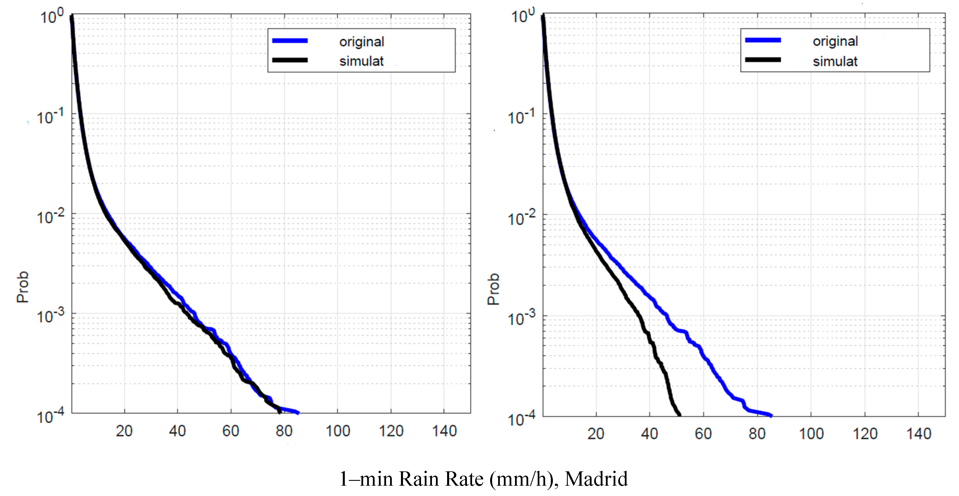
Figure 15.
Prague. Probability distrbution that the 1–min rain rate in abscissa is exceeded in the experimental data, , blue line, and in the simulated 1–min data, , black line. Left panel: is obtained by using local values of the conditional PDFs; Right panel: is obtained by using Spino d’Adda conditional PDFs (Table 2).
Figure 15.
Prague. Probability distrbution that the 1–min rain rate in abscissa is exceeded in the experimental data, , blue line, and in the simulated 1–min data, , black line. Left panel: is obtained by using local values of the conditional PDFs; Right panel: is obtained by using Spino d’Adda conditional PDFs (Table 2).
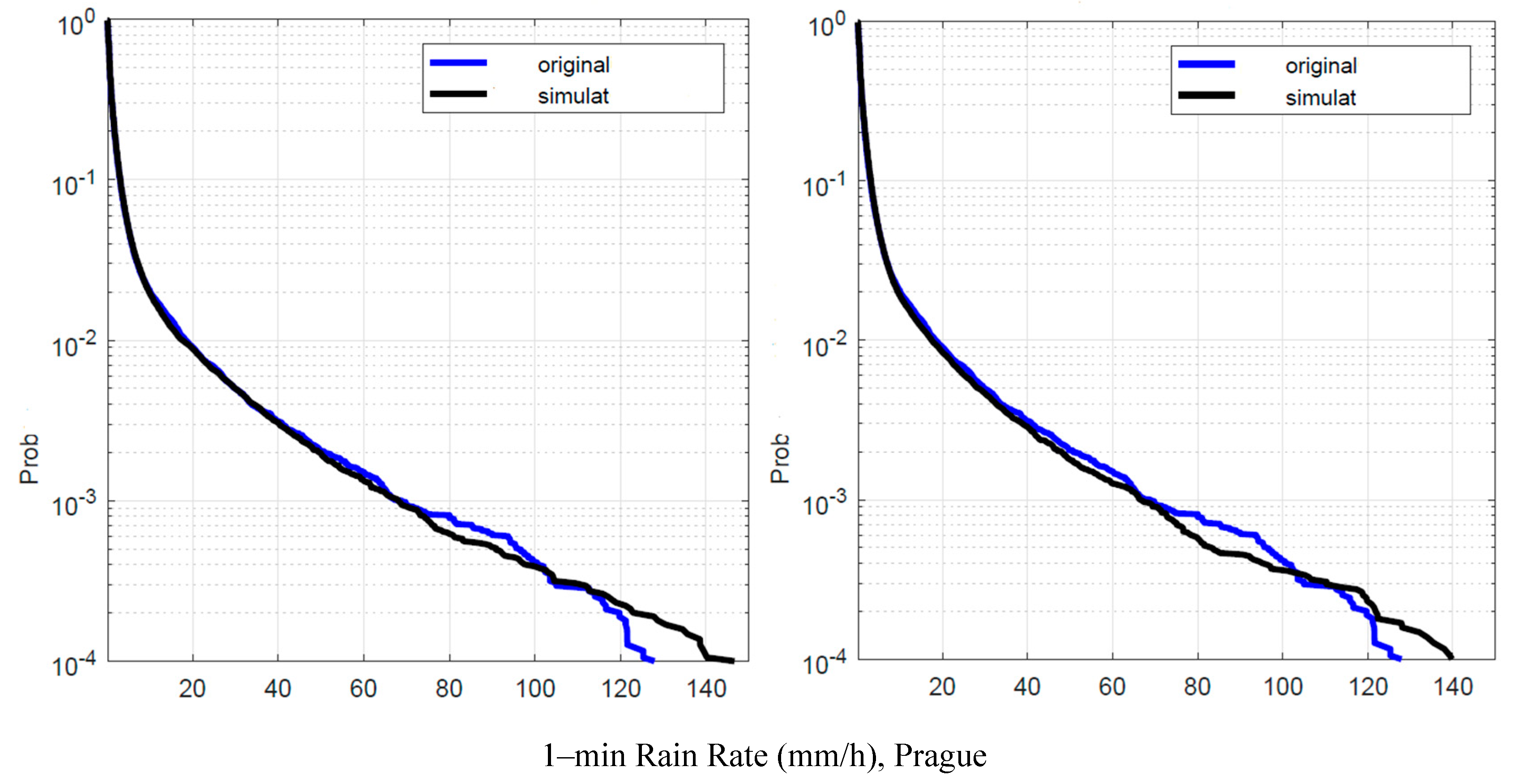
Figure 16.
Tampa. Probability distrbution that the 1–min rain rate in abscissa is exceeded in the experimental data, , blue line, and in the simulated 1–min data, , black line. Left panel: is obtained by using local values of the conditional PDFs; Right panel: is obtained by using Spino d’Adda conditional PDFs (Table 2).
Figure 16.
Tampa. Probability distrbution that the 1–min rain rate in abscissa is exceeded in the experimental data, , blue line, and in the simulated 1–min data, , black line. Left panel: is obtained by using local values of the conditional PDFs; Right panel: is obtained by using Spino d’Adda conditional PDFs (Table 2).
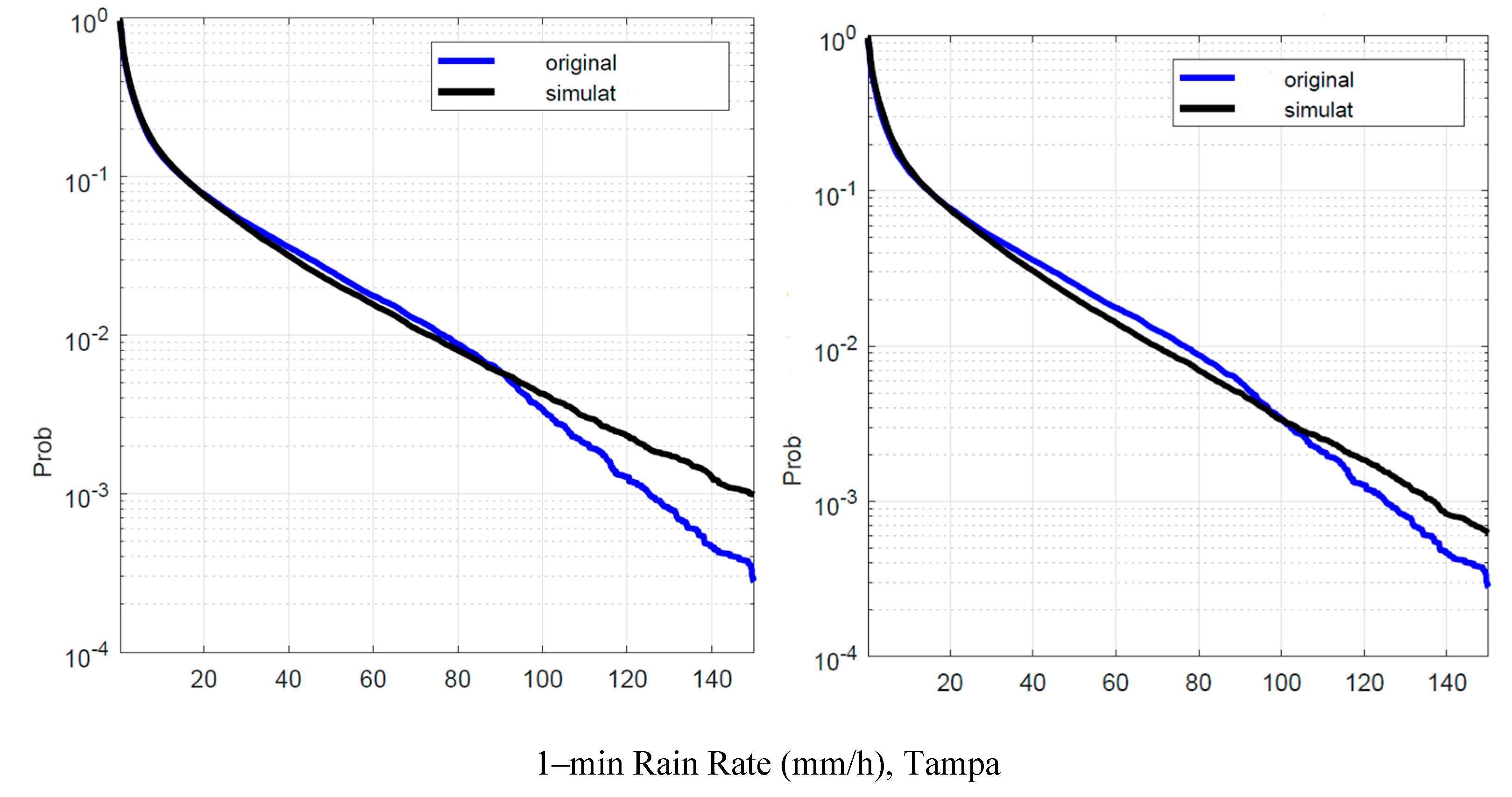
Figure 16.
White Sands. Probability distrbution that the 1–min rain rate in abscissa is exceeded in the experimental data, , blue line, and in the simulated 1–min data, , black line. Left panel: is obtained by using local values of the conditional PDFs; Right panel: is obtained by using Spino d’Adda conditional PDFs (Table 2).
Figure 16.
White Sands. Probability distrbution that the 1–min rain rate in abscissa is exceeded in the experimental data, , blue line, and in the simulated 1–min data, , black line. Left panel: is obtained by using local values of the conditional PDFs; Right panel: is obtained by using Spino d’Adda conditional PDFs (Table 2).
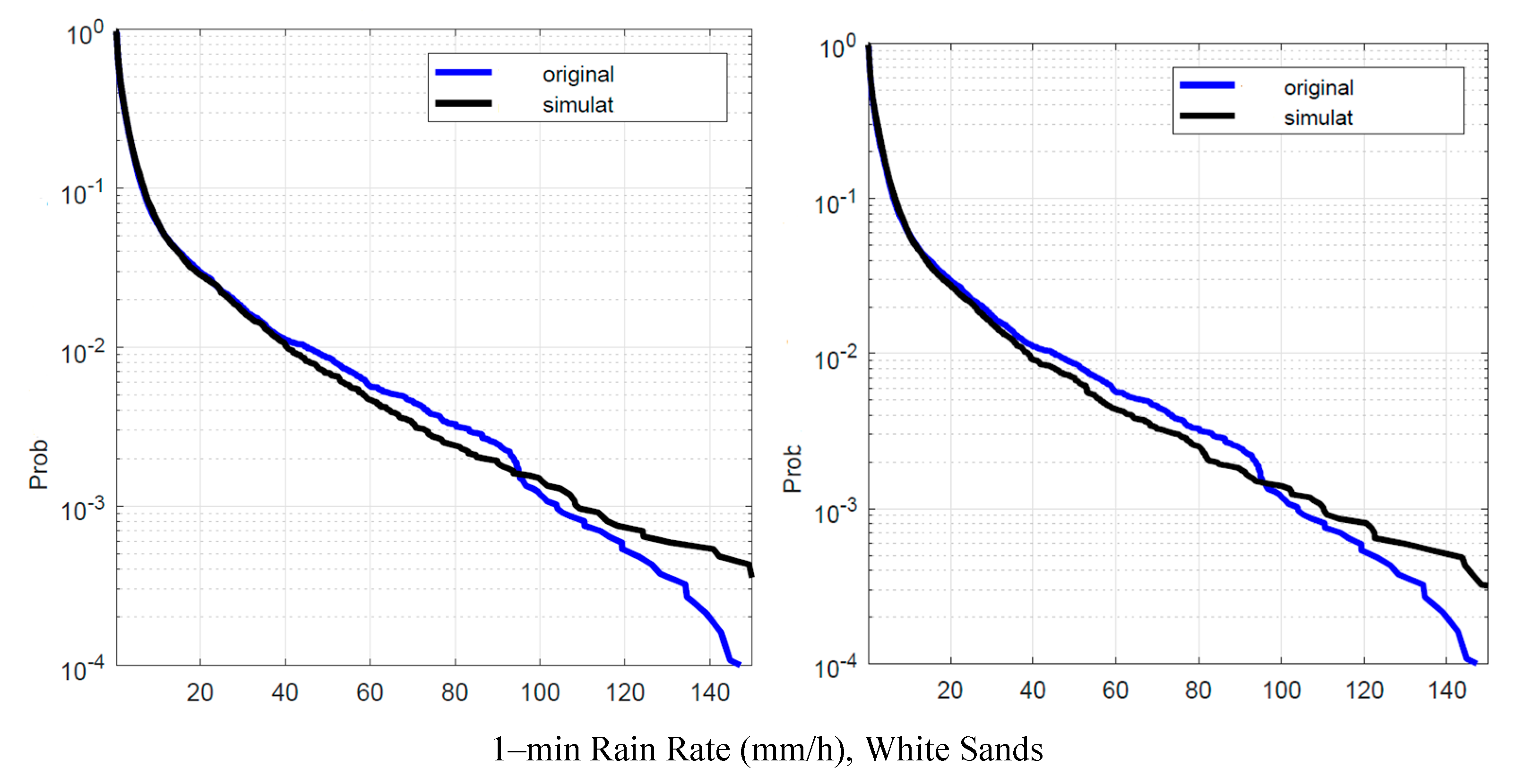
Figure 17.
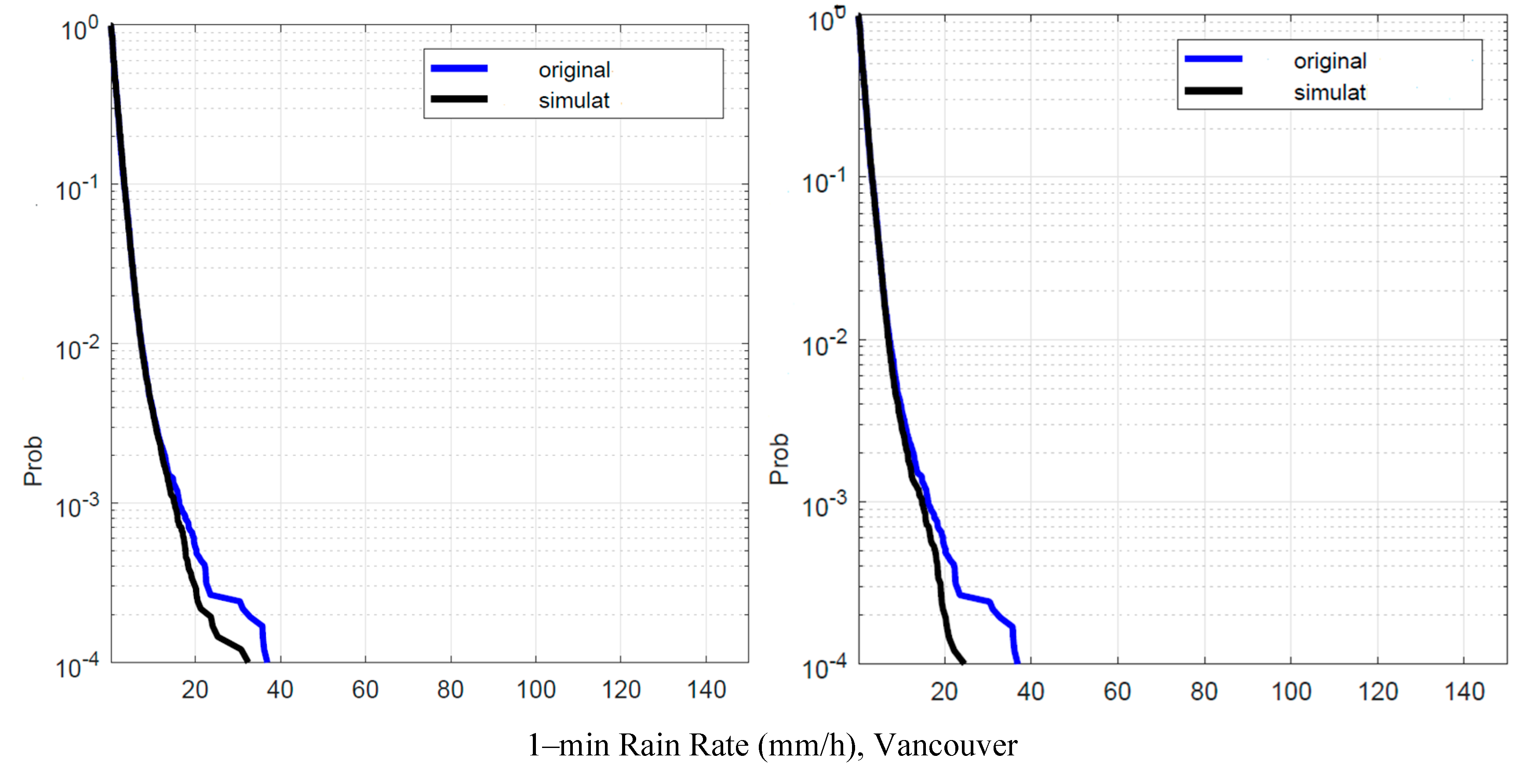
Vancouver. Probability distrbution that the 1–min rain rate in abscissa is exceeded in the experimental data, , blue line, and in the simulated 1–min data, , black line. Left panel: is obtained by using local values of the conditional PDFs; Right panel: is obtained by using Spino d’Adda conditional PDFs (Table 2).
Figure 17.
Vancouver. Probability distrbution that the 1–min rain rate in abscissa is exceeded in the experimental data, , blue line, and in the simulated 1–min data, , black line. Left panel: is obtained by using local values of the conditional PDFs; Right panel: is obtained by using Spino d’Adda conditional PDFs (Table 2).
In the next section, as an example of the possible applications, we apply the theory to the important case of estimating the rain attenuation in slant paths to satellites in the Geostationary orbit with a powerful tool, the Synthetic Storm Technique.
5. Rain Attenuation in Slant Paths to Geostationary Satellites: The Synthetic Storm Technique
In this section, as an example of the possible applications of the conversion of into , we use the theory to estimate the rain attenuation in slant paths to geostationary satellites by using the a very reliable tool available today, namely the Synthetic Storm Technique (SST), which need as input 1–min rain–rate time series [1]. We first recall briefly the SST theory and then we appply it to the sites of Table 1, by simulating, at each site, reliable rain attenuation time series in 35.5° slant paths to a geostationary satellite with a 20.7 GHz carrier, circular polarization of the electromagnetic wave.
5.1. Synthetic Storm Technique
Satellite communication links at centimeter and millimeter wave frequencies are faded by rainfall. For a reliable link‒budget design, we need to know, at the very least, the annual probability distribution function – i.e. the fraction of time in an average year – of rain attenuation (dB) measured/predicted in the up‒ or down‒links to a satellite. Instead of long and expensive measurements of beacon attenuation, prediction models are used for estimating from locally, measured or estimated, annual probability distributions, of 1‒min rain rate . The Synthetic Storm Technique [1] is a powerful and accurate tool, as is now recognized, that can produce all the necessary statistics of rain attenuation, not only , but also fade durations and rate of change of attenuation because it provides reliable rain attenuation time series and their power spectra [15,16]. From knowing the rain‒rate time series (mm/h), recorded at a site, the SST can generate rain attenuation time series , with time resolution of the order of one second – at any frequency and polarization, and for any slant path above about 10°. Because it reproduces reliable , it has been used in the last 30 years for many purposes, by several researchers [17,18,19,20,21,22,23,24]. In this paper we consider only ; fade durations and rate–of–change will be studied in a future work.
5.2. Application of the SST to All Sites
We apply the SST twice: first by using as input the experimental 1–min rain–rate time series, namely , secondly by using the simulated . Figure 10 shows the annual average rain–attenuation probability distributions obtained with and with . There are no appreciable differences that can impact on satellite system design.
Figure 18.
Average annual probability distrbution – namely, the fraction of time of a year – that the rain attenuation (dB) in abscissa is exceeded, estimated with the SST; cyan line: experimental , magenta line: simulated .
Figure 18.
Average annual probability distrbution – namely, the fraction of time of a year – that the rain attenuation (dB) in abscissa is exceeded, estimated with the SST; cyan line: experimental , magenta line: simulated .
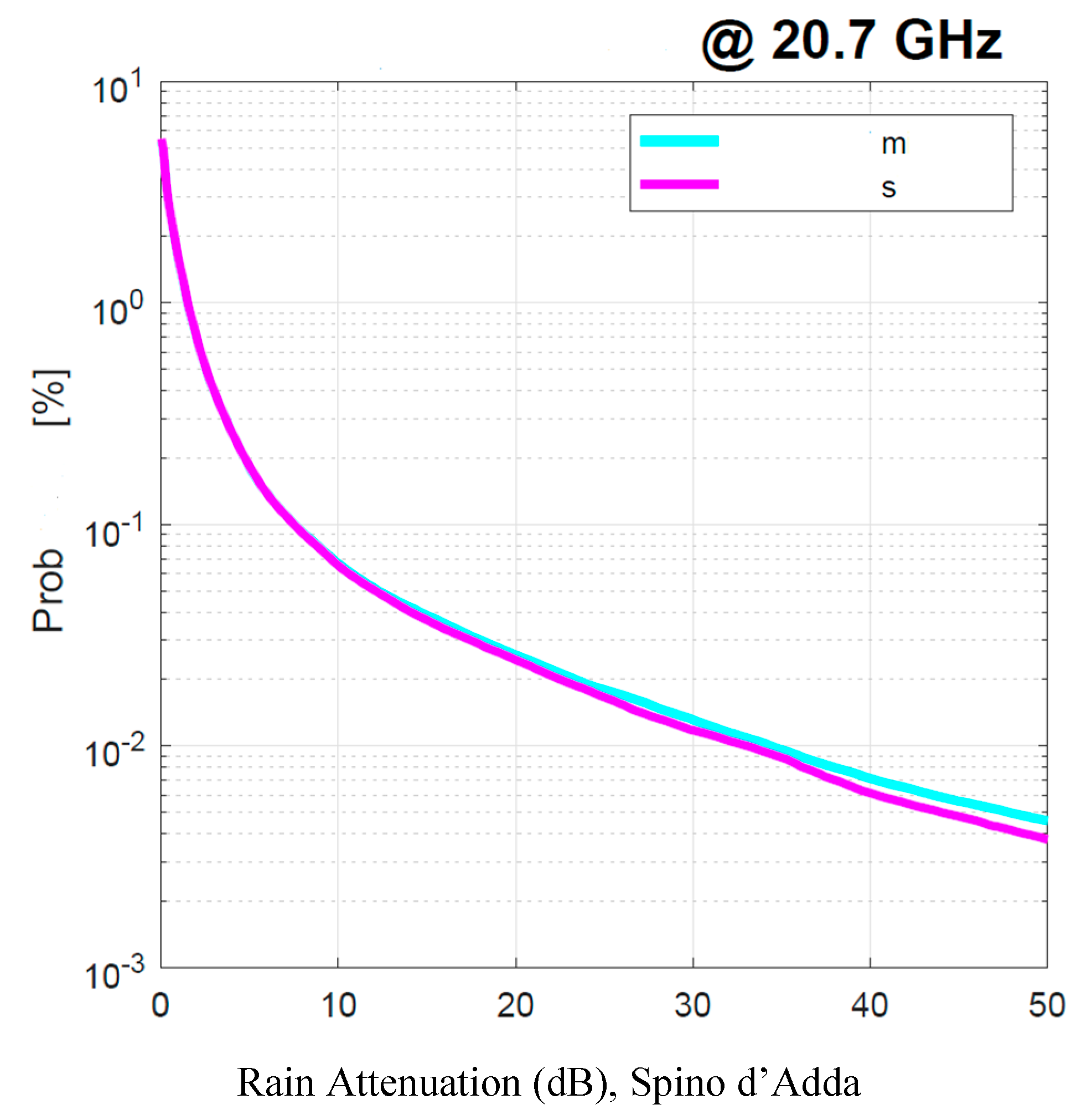
Figure 18.
Gera Lario. Average annual probability distrbution that the rain attenuation (dB) in abscissa is exceeded, estimated with the SST; blue line: experimental , black line: simulated . Left panel: is obtained by using local values of the conditional rain rate PDFs; Right panel: is obtained by using Spino d’Adda conditional PDFs (Table 2).
Figure 18.
Gera Lario. Average annual probability distrbution that the rain attenuation (dB) in abscissa is exceeded, estimated with the SST; blue line: experimental , black line: simulated . Left panel: is obtained by using local values of the conditional rain rate PDFs; Right panel: is obtained by using Spino d’Adda conditional PDFs (Table 2).

Figure 19.
Fucino. Average annual probability distrbution that the rain attenuation (dB) in abscissa is exceeded, estimated with the SST; blue line: experimental , black line: simulated . Left panel: is obtained by using local values of the conditional rain rate PDFs; Right panel: is obtained by using Spino d’Adda conditional PDFs (Table 2).
Figure 19.
Fucino. Average annual probability distrbution that the rain attenuation (dB) in abscissa is exceeded, estimated with the SST; blue line: experimental , black line: simulated . Left panel: is obtained by using local values of the conditional rain rate PDFs; Right panel: is obtained by using Spino d’Adda conditional PDFs (Table 2).
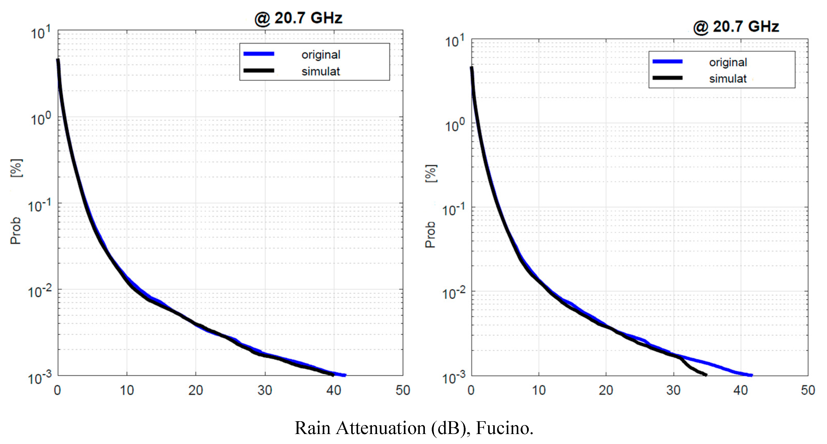
Figure 20.
Madrid. Average annual probability distrbution that the rain attenuation (dB) in abscissa is exceeded, estimated with the SST; blue line: experimental , black line: simulated . Left panel: is obtained by using local values of the conditional rain rate PDFs; Right panel: is obtained by using Spino d’Adda conditional PDFs (Table 2).
Figure 20.
Madrid. Average annual probability distrbution that the rain attenuation (dB) in abscissa is exceeded, estimated with the SST; blue line: experimental , black line: simulated . Left panel: is obtained by using local values of the conditional rain rate PDFs; Right panel: is obtained by using Spino d’Adda conditional PDFs (Table 2).
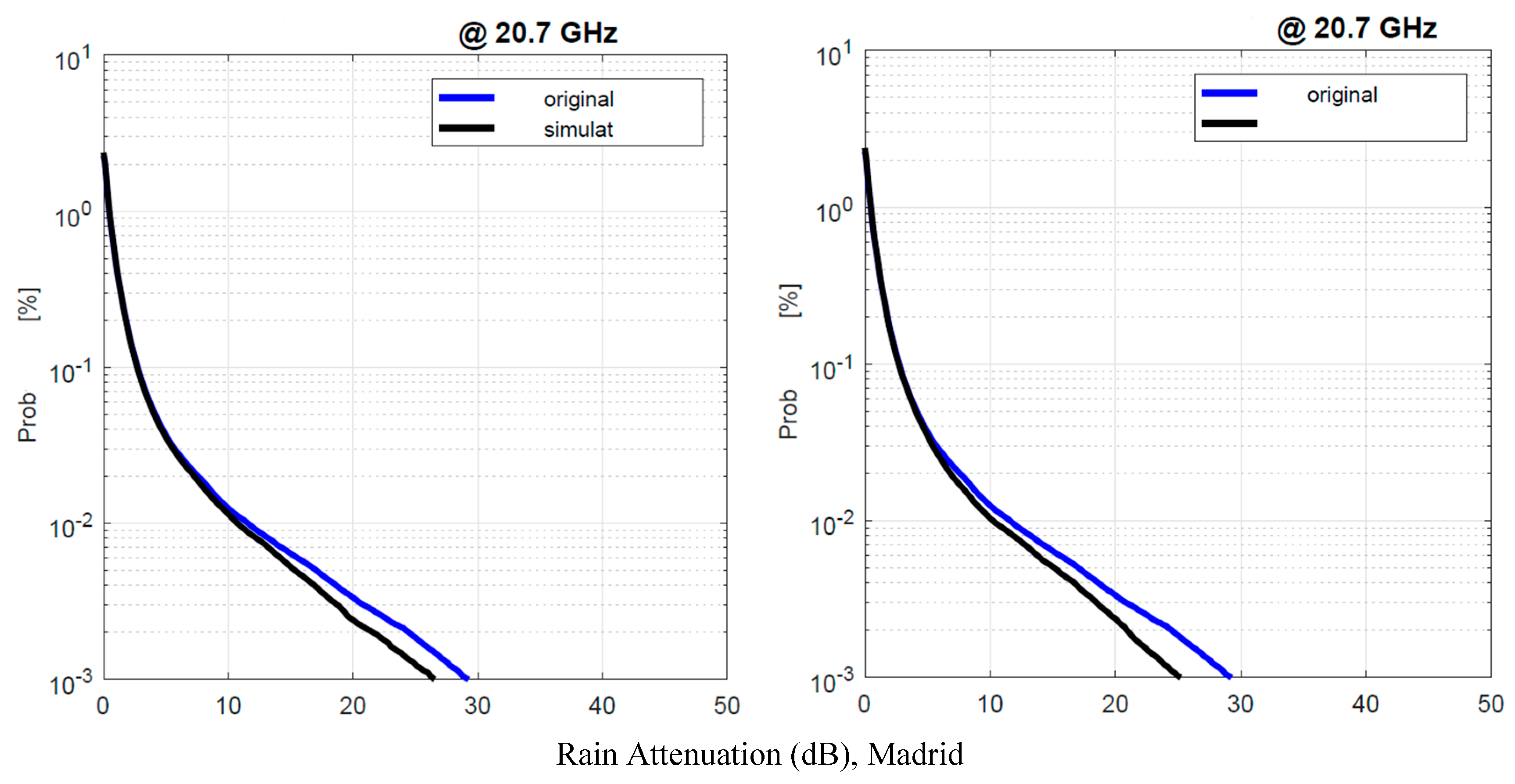
Figure 21.
Prague. Average annual probability distrbution that the rain attenuation (dB) in abscissa is exceeded, estimated with the SST; blue line: experimental , black line: simulated . Left panel: is obtained by using local values of the conditional rain rate PDFs; Right panel: is obtained by using Spino d’Adda conditional PDFs (Table 2).
Figure 21.
Prague. Average annual probability distrbution that the rain attenuation (dB) in abscissa is exceeded, estimated with the SST; blue line: experimental , black line: simulated . Left panel: is obtained by using local values of the conditional rain rate PDFs; Right panel: is obtained by using Spino d’Adda conditional PDFs (Table 2).
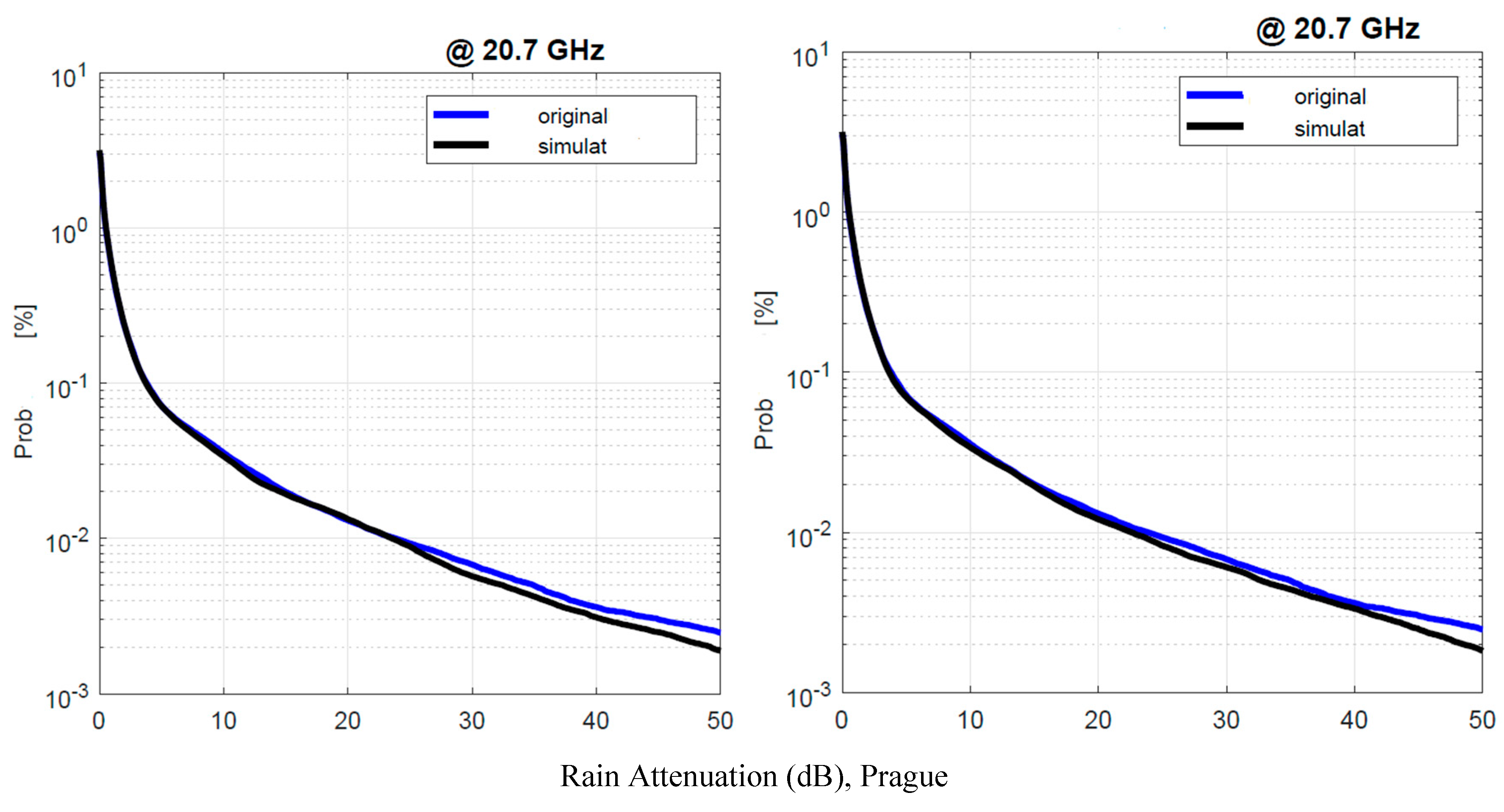
Figure 22.
Tampa. Average annual probability distrbution that the rain attenuation (dB) in abscissa is exceeded, estimated with the SST; blue line: experimental , black line: simulated . Left panel: is obtained by using local values of the conditional rain rate PDFs; Right panel: is obtained by using Spino d’Adda conditional PDFs (Table 2).
Figure 22.
Tampa. Average annual probability distrbution that the rain attenuation (dB) in abscissa is exceeded, estimated with the SST; blue line: experimental , black line: simulated . Left panel: is obtained by using local values of the conditional rain rate PDFs; Right panel: is obtained by using Spino d’Adda conditional PDFs (Table 2).
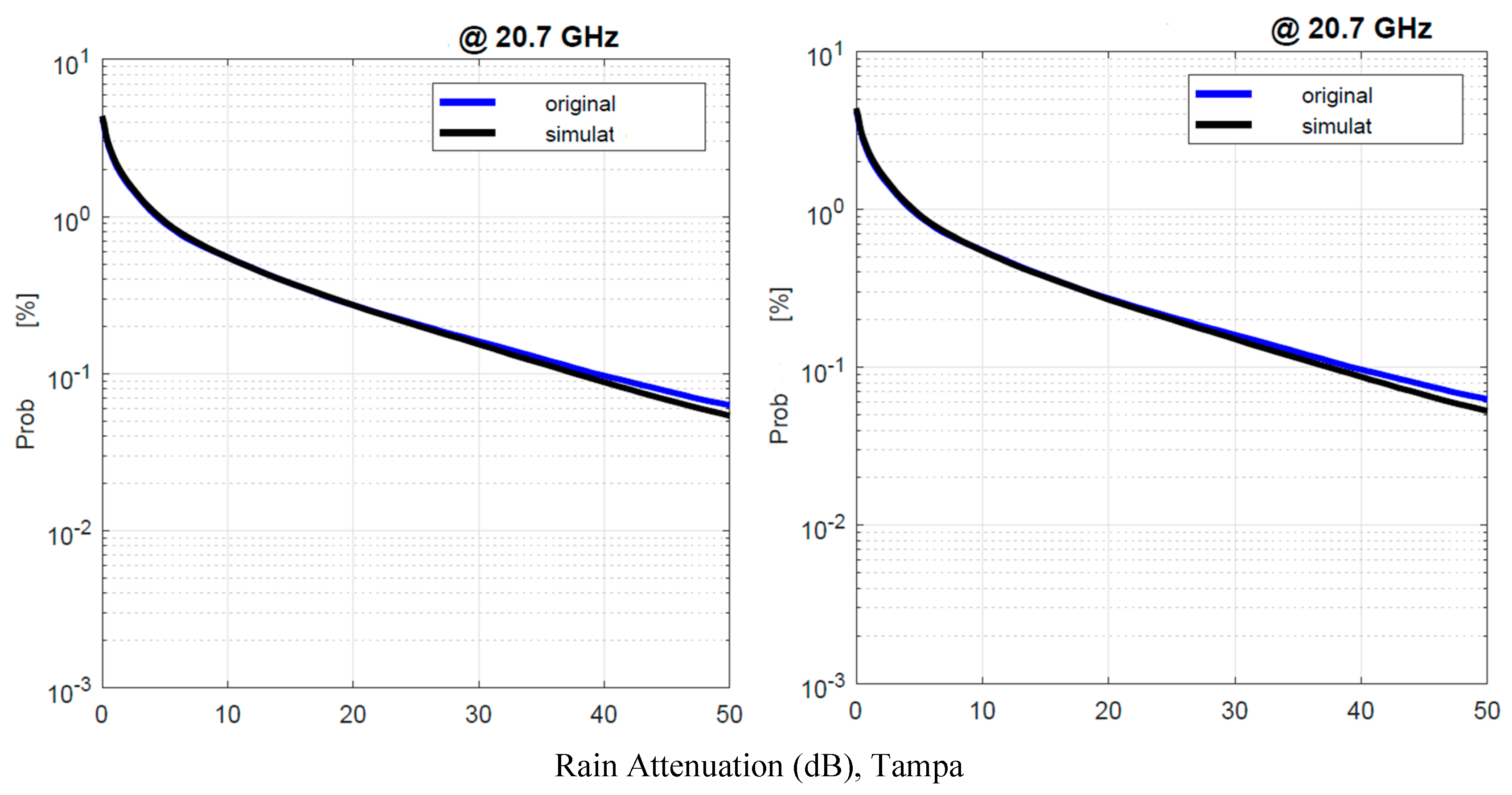
Figure 23.
White Sands. Average annual probability distrbution that the rain attenuation (dB) in abscissa is exceeded, estimated with the SST; blue line: experimental , black line: simulated . Left panel: is obtained by using local values of the conditional rain rate PDFs; Right panel: is obtained by using Spino d’Adda conditional PDFs (Table 2).
Figure 23.
White Sands. Average annual probability distrbution that the rain attenuation (dB) in abscissa is exceeded, estimated with the SST; blue line: experimental , black line: simulated . Left panel: is obtained by using local values of the conditional rain rate PDFs; Right panel: is obtained by using Spino d’Adda conditional PDFs (Table 2).
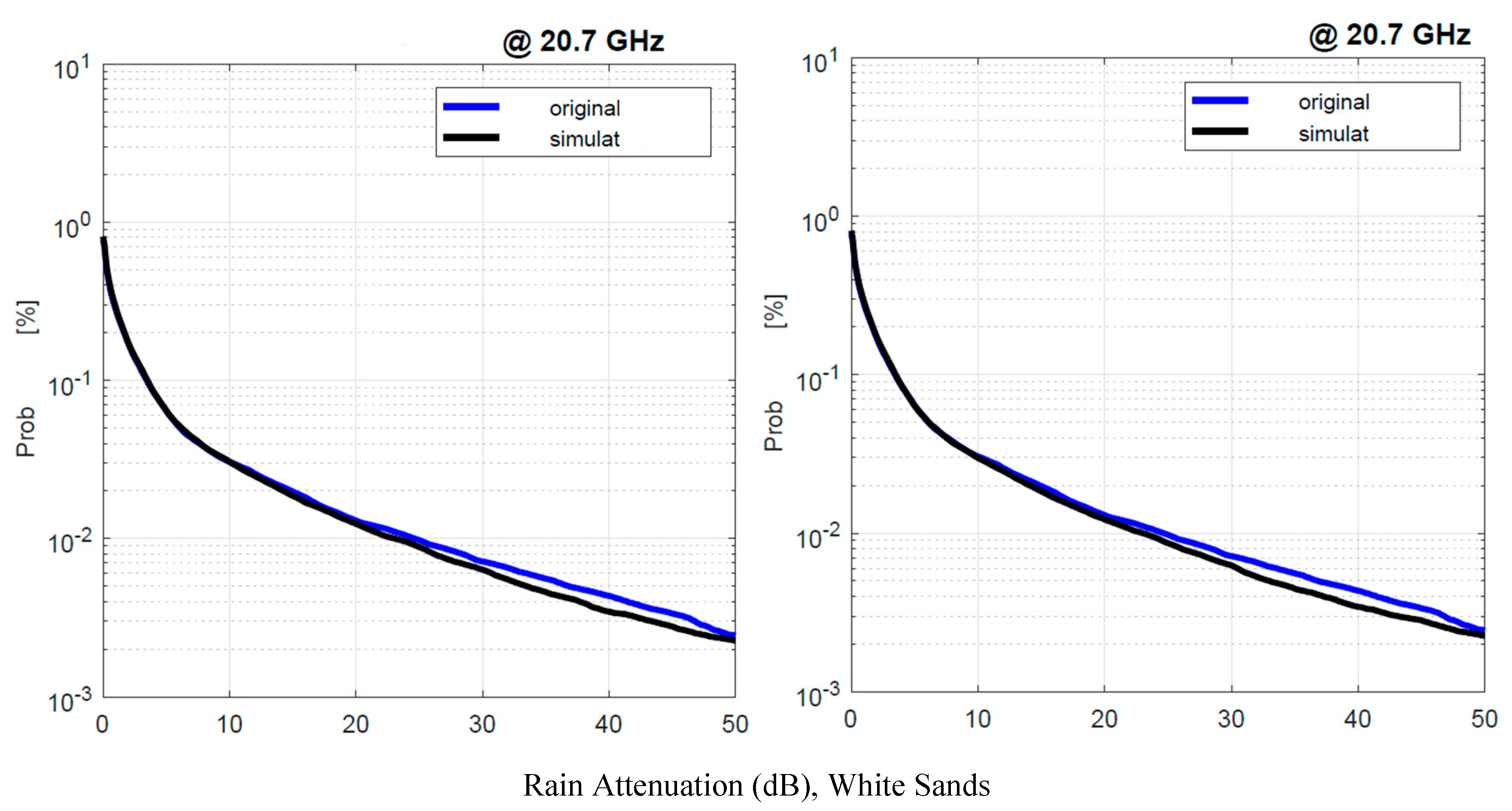
Figure 24.
Vancouver. Average annual probability distrbution that the rain attenuation (dB) in abscissa is exceeded, estimated with the SST; blue line: experimental , black line: simulated . Left panel: is obtained by using local values of the conditional rain rate PDFs; Right panel: is obtained by using Spino d’Adda conditional PDFs (Table 2).
Figure 24.
Vancouver. Average annual probability distrbution that the rain attenuation (dB) in abscissa is exceeded, estimated with the SST; blue line: experimental , black line: simulated . Left panel: is obtained by using local values of the conditional rain rate PDFs; Right panel: is obtained by using Spino d’Adda conditional PDFs (Table 2).
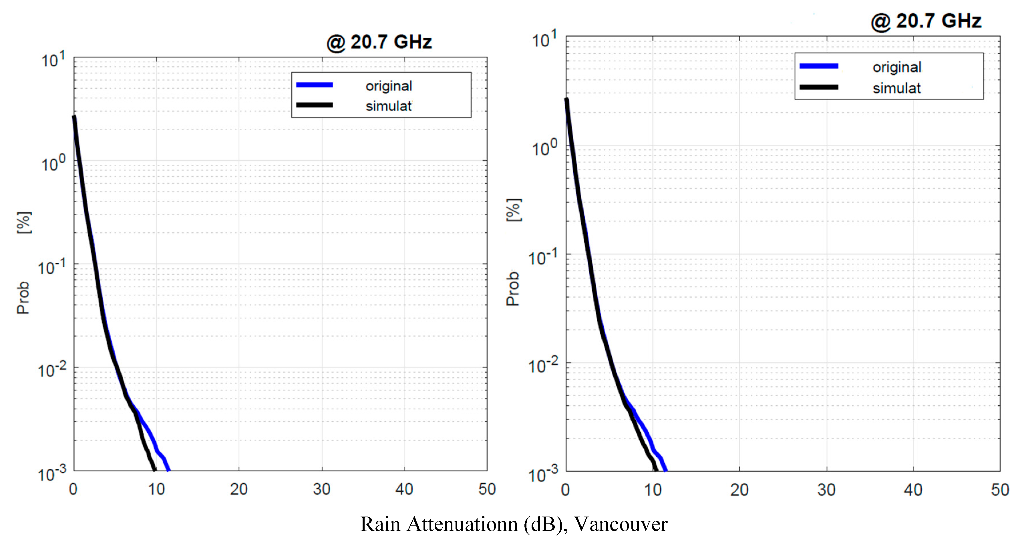
Now, since for satellite communications the tolerated outage probabilty due to rain attenuation, i.e. , is in the range (%) (i.e. outage time from 525 to 52.5 minutes, respectively), from these figures it turns out that for most probability range there are no signficant differences between rain attenuation estimated with local or with Spino d’Adda parameters.
5. Conclusions
We have developed a method –a filtered Markov process – to convert 10–min rain–rate time series into 1–min rain–rate time series, the latter to be used as input to the Synthetic Storm Technique for calculating rain–attenuation time series in satellite communication systems, in hydrology and to estimate runoff, erosiont, pollutant transport. The rationale for the need of such a method lies in the fact that now several meteorological services make available time series of quantity of water collected every 10 minutes, compared to the past when, at most, the quantity referred to 1 hour. To develop and validate the method, we have used a very large data bank of 1–min rain–rate time series, collected in sites of different climatic conditions, which we have converted into 10–min time series to simulate the alleged data provided by meteorological services. From them, we have estimateof the original 1–min rain rate time seies. The simulated 1–min rain–rate time series are very similar to the original ones, therefore we think that the method can be reliably used in the fields mentioned above.
In conclusion, we have reached two important results:
- a)
- The conversion of into is very accurate, even using the rain rate conversion parameters of Spino d’Adda.
- b)
- obtained by using as SST input the rain rate parameters of Spino d’Adda is indistinguishable with that simulated with the local conversion parameters, in a large probability range useful for practical applications in satellite communications.
Author Contributions
Conceptualization, E.M..; methodology, E.M..; software, E.M. and C.R.; validation, E.M. and C.R.; investigation, E.M. and C.R.; data curation, E.M. and C.R.; writing—original draft preparation, E.M. and C.R.; writing—review and editing, E.M. and C.R.; visualization, E.M. and C.R.; All authors have read and agreed to the published version of the manuscript.
Funding
This research received no external funding.
Institutional Review Board Statement
Not applicable.
Informed Consent Statement
Not applicable.
Data Availability Statement
Data are available upon request to the authors.
Acknowledgments
We wish to thank Roberto Acosta, at NASA years ago, for providing the rain rate data of Tampa; Ondrej Fiser, Institute of Atmospheric Physics in Prague, for providing the rain rate data of Prague; José Manuel Riera, Universidad Politécnica de Madrid, for providing the rain rate data of Madrid.
Conflicts of Interest
The authors declare no conflicts of interest.
Appendix A. List of Mathematical Symbols
| Symbol | Definition |
| Rain attenuation | |
| Digital filter cut–off frequency | |
| Nyquist frequency | |
| Optimum digital filter cut–off frequency | |
| Log average value | |
| Log conditonal average value | |
| Quantity of water accumulated in 10 minutes, experimental | |
| Quantity of water accumulated in 10 minutes, simulated | |
| Quantity of water accumulated in 10 minutes, simulated and filtered. | |
| Annual average probability distribution of rain attenuation, simulated | |
| Probability distribution of 1–min rain rate, experimental | |
| Probability distribution of 1–min rain rate, simulated | |
| 1–min rain rate time series, experimental | |
| 10–min rain rate time series, experimental | |
| 1–min rain rate time series, simulated, not filtered, not scaled | |
| 1–min rain rate time series, simulated, not filtered, scaled | |
| 1–min rain rate time series, simulated, filtered, scaled | |
| 1–min rain rate time series, simulated, double–filtered, scaled: final simulated time series. | |
| Log standard deviation | |
| Conditional log standard deviation | |
| standard Gaussian random variable | |
| Denormalized Gaussian random variable | |
| error at equal probability |
Appendix B. Conditional PDFs Parameters
Table A1.
Gera Lario. Mean value, standard deviation of and correlation coefficient between two successive samples within the same 10–min interval, for the indicated ranges. The first range starts at 0.2 mm/h.
Table A1.
Gera Lario. Mean value, standard deviation of and correlation coefficient between two successive samples within the same 10–min interval, for the indicated ranges. The first range starts at 0.2 mm/h.
| (mm/h) | Mean | Standard Deviation | Correlation Coefficient |
| 0–2 | –0.68 | 0.81 | 0.94 |
| 2–4 | 0.94 | 0.46 | 0.71 |
| 4–6 | 1.50 | 0.45 | 0.65 |
| 6–8 | 1.82 | 0.55 | 0.63 |
| 8–10 | 2.08 | 0.54 | 0.71 |
| 10–15 | 2.30 | 0.77 | 0.70 |
| 15–20 | 2.64 | 0.78 | 0.66 |
| 20–30 | 3.02 | 0.71 | 0.73 |
| 30–40 | 3.20 | 1.03 | 0.58 |
| > 40 | 3.64 | 1.07 | 0.72 |
Table A2.
Fucino. Mean value, standard deviation of and correlation coefficient between two successive samples within the same 10–min interval, for the indicated ranges. The first range starts at 0.2 mm/h.
Table A2.
Fucino. Mean value, standard deviation of and correlation coefficient between two successive samples within the same 10–min interval, for the indicated ranges. The first range starts at 0.2 mm/h.
| (mm/h) | Mean | Standard Deviation | Correlation Coefficient |
| 0–2 | –0.69 | 0.79 | 0.92 |
| 2–4 | 0.91 | 0.53 | 0.67 |
| 4–6 | 1.47 | 0.51 | 0.65 |
| 6–8 | 1.83 | 0.50 | 0.63 |
| 8–10 | 2.08 | 0.51 | 0.60 |
| 10–15 | 2.33 | 0.59 | 0.61 |
| 15–20 | 2.63 | 0.78 | 0.58 |
| 20–30 | 2.86 | 0.97 | 0.61 |
| 30–40 | 2.80 | 0.95 | 0.75 |
| > 40 | 3.77 | 0.92 | 0.75 |
Table A3.
Madrid. Mean value, standard deviation of and correlation coefficient between two successive samples within the same 10–min interval, for the indicated ranges. The first range starts at 0.2 mm/h.
Table A3.
Madrid. Mean value, standard deviation of and correlation coefficient between two successive samples within the same 10–min interval, for the indicated ranges. The first range starts at 0.2 mm/h.
| (mm/h) | Mean | Standard Deviation | Correlation Coefficient |
| 0–2 | –0.36 | 0.66 | 0.85 |
| 2–4 | 0.90 | 0.50 | 0.70 |
| 4–6 | 1.43 | 0.59 | 0.68 |
| 6–8 | 1.77 | 0.63 | 0.65 |
| 8–10 | 1.97 | 0.77 | 0.60 |
| 10–15 | 2.16 | 0.96 | 0.66 |
| 15–20 | 2.49 | 0.98 | 0.68 |
| 20–30 | 2.85 | 0.96 | 0.73 |
| 30–40 | 3.25 | 0.95 | 0.78 |
| > 40 | 3.57 | 0.78 | 0.72 |
Table A4.
Prague. Mean value, standard deviation of and correlation coefficient between two successive samples within the same 10–min interval, for the indicated ranges. The first range starts at 0.2 mm/h.
Table A4.
Prague. Mean value, standard deviation of and correlation coefficient between two successive samples within the same 10–min interval, for the indicated ranges. The first range starts at 0.2 mm/h.
| (mm/h) | Mean | Standard Deviation | Correlation Coefficient |
| 0–2 | –0.70 | 0.74 | 0.91 |
| 2–4 | 0.91 | 0.52 | 0.72 |
| 4–6 | 1.47 | 0.55 | 0.65 |
| 6–8 | 1.71 | 0.74 | 0.61 |
| 8–10 | 2.02 | 0.67 | 0.77 |
| 10–15 | 2.25 | 0.87 | 0.7 |
| 15–20 | 2.63 | 0.76 | 0.56 |
| 20–30 | 2.87 | 1.16 | 0.75 |
| 30–40 | 3.32 | 0.74 | 0.68 |
| > 40 | 3.90 | 0.83 | 0.69 |
Table A5.
Tampa. Mean value, standard deviation of and correlation coefficient between two successive samples within the same 10–min interval, for the indicated ranges. The first range starts at 0.2 mm/h.
Table A5.
Tampa. Mean value, standard deviation of and correlation coefficient between two successive samples within the same 10–min interval, for the indicated ranges. The first range starts at 0.2 mm/h.
| (mm/h) | Mean | Standard Deviation | Correlation Coefficient |
| 0–2 | –0.50 | 0.77 | 0.82 |
| 2–4 | 0.90 | 0.62 | 0.69 |
| 4–6 | 1.40 | 0.70 | 0.71 |
| 6–8 | 1.63 | 0.94 | 0.70 |
| 8–10 | 1.93 | 0.83 | 0.69 |
| 10–15 | 2.20 | 0.91 | 0.67 |
| 15–20 | 2.49 | 1.01 | 0.70 |
| 20–30 | 2.94 | 0.88 | 0.69 |
| 30–40 | 3.25 | 0.91 | 0.71 |
| > 40 | 3.87 | 0.81 | 0.69 |
Table A6.
White Sands. Mean value, standard deviation of and correlation coefficient between two successive samples within the same 10–min interval, for the indicated ranges. The first range starts at 0.2 mm/h.
Table A6.
White Sands. Mean value, standard deviation of and correlation coefficient between two successive samples within the same 10–min interval, for the indicated ranges. The first range starts at 0.2 mm/h.
| (mm/h) | Mean | Standard Deviation | Correlation Coefficient |
| 0–2 | –0.58 | 0.75 | 0.85 |
| 2–4 | 0.93 | 0.51 | 0.68 |
| 4–6 | 1.49 | 0.6 | 0.67 |
| 6–8 | 1.78 | 0.69 | 0.69 |
| 8–10 | 1.99 | 0.71 | 0.68 |
| 10–15 | 2.15 | 1.05 | 0.72 |
| 15–20 | 2.6 | 0.8 | 0.69 |
| 20–30 | 2.88 | 0.91 | 0.65 |
| 30–40 | 3.48 | 0.51 | 0.75 |
| > 40 | 3.88 | 0.71 | 0.69 |
Table A7.
Vancouver. Mean value, standard deviation of and correlation coefficient between two successive samples within the same 10–min interval, for the indicated ranges. The first range starts at 0.2 mm/h.
Table A7.
Vancouver. Mean value, standard deviation of and correlation coefficient between two successive samples within the same 10–min interval, for the indicated ranges. The first range starts at 0.2 mm/h.
| (mm/h) | Mean | Standard Deviation | Correlation Coefficient |
| 0–2 | –0.40 | 0.71 | 0.92 |
| 2–4 | 0.93 | 0.37 | 0.74 |
| 4–6 | 1.52 | 0.37 | 0.70 |
| 6–8 | 1.78 | 0.49 | 0.55 |
| 8–10 | 2.05 | 0.48 | 0.60 |
| 10–15 | 2.42 | 0.52 | 0.75 |
| 15–20 | 2.59 | 0.58 | 0.69 |
| 20–30 | 2.72 | 0.96 | 0.82 |
| 30–40 | –– | –– | –– |
| > 40 | –– | –– | –– |
References
- Matricciani, E. Physical–mathematical model of the dynamics of rain attenuation based on rain–rate time series and a two–layer vertical structure of precipitation. Radio Sci. 1996, 31, 281–295. [Google Scholar] [CrossRef]
- Matricciani, E.; Riva, C. The search for the most reliable long‒term rain attenuation cdf of a slant path and the impact on pre‒diction models. IEEE Trans. Antennas Propag. 2005, 53, 3075–3079. [Google Scholar] [CrossRef]
- Matricciani, E. A Mathematical Theory of De–Integrating Long–Time Integrated Rainfall and Its Application for Predicting 1–Min Rain Rate Statistics. International Journal of Satellite Communication and Networking 2011, 29, 501–530. [Google Scholar] [CrossRef]
- Matricciani, E. A mathematical theory of de–integrating long–time integrated rainfall statistics. Part II: from 1 day to 1 minute. International Journal of Satellite Communications and Networking 2013, 31, 77–102. [Google Scholar] [CrossRef]
- Connolly, R.D.; Schirmer, J.; Dunn, P.K. A daily rainfall disaggregation model. Agricultural and Forest Meteorology 1998, 92, 105–117. [Google Scholar] [CrossRef]
- Salles, C.; Poesen, J.; Sempere-Torres, D. Kinetic energy and its functional relationship with intensity. Journal of Hydrology. 2002, 257, 256–270. [Google Scholar] [CrossRef]
- Van Dijk, A.I.J.M.; Bruijnzeel, L.A.; Rosewell, C.J. Rainfall intensity–kinetic energy relationships: a critical literature appraisal. Journal of Hydrology 2002, 261, 1–23. [Google Scholar] [CrossRef]
- Ali, S.; Rahman, A.; Shaik, R. A Review of Event–Based Conceptual Rainfall–Runoff Models: A Case for Australia. Encyclopedia 2024, 4, 966–983. [Google Scholar] [CrossRef]
- Papoulis Papoulis, A. Probability & Statistics; Prentice Hall: Hoboken, NJ, USA, 1990. [Google Scholar]
- Lindgren, B.W. Statistical Theory, 2nd ed.; MacMillan Company: New York, NY, USA, 1968. [Google Scholar]
- Bury, K.V. (1975), Statistical Models in Applied Science, John Wiley.
- Kleinrock, L. Queueing Systems, John Wiley & Sons: New York, USA. 1975.
- Haykin, S.; Van Veen, B. Signals and Systems, 2nd ed.; John Wiley & Sons: New York, USA, 2003. [Google Scholar]
- Haykin, S. Communication Sysyems, 4th ed.; John Wiley & Sons: New York, USA, 2001. [Google Scholar]
- Matricciani, E. Prediction of fade durations due to rain in satellite communication systems. Radio Sci. 1997, 32, 935–941. [Google Scholar] [CrossRef]
- Matricciani, E. Physical–mathematical model of dynamics of rain attenuation with application to power spectrum. Electron. Lett. 1994, 30, 522–524. [Google Scholar] [CrossRef]
- Kanellopoulos, S.; Panagopoulos, A.; Matricciani, E.; Kanellopoulos, J. Annual and Diurnal Slant Path Rain Attenuation Statistics in Athens Obtained With the Synthetic Storm Technique. IEEE Trans. Antennas Propag. 2006, 54, 2357–2364. [Google Scholar] [CrossRef]
- Sánchez‒Lago, I.; Fontán, F.P.; Mariño, P.; Fiebig, U.C. Validation of the Synthetic Storm Technique as Part of a Time‒Series Generator for Satellite Links. IEEE Antennas Wirel. Propag. Lett. 2007, 6, 372–375. [Google Scholar] [CrossRef]
- Mahmudah, H.; Wijayanti, A.; Mauludiyanto, A.; Hendrantoro, G.; Matsushima, A. Analysis of Tropical Attenuation Statistics using Synthetic Storm for Millimeter‒Wave Wireless Network Design. In Proceedings of the 5th IFIP International Conference on Wireless and Optical Communications Networks (WOCN ’08), Surabaya, East Java, Indonesia, 5‒7 May 2008. [Google Scholar]
- Lyras, N.K.; Kourogiorgas, C.I.; Panagopoulos, A.D.; Ventouras, S. Rain Attenuation Statistics at Ka and Q band in Athens using SST and Short Scale Dynamic Diversity Gain Evaluation. In Proceedings of the 2016 Loughborough Antennas & Propagation Conference (LAPC), Loughborough, UK, 14–15 November 2016. [Google Scholar]
- Nandi, A. Prediction of Rain Attenuation Statistics from Measured Rain Rate Statistics using Synthetic Storm Technique for Micro and Millimeter Wave Communication Systems. In Proceedings of the 2018 IEEE MTT‒S International Microwave and RF Conference (IMaRC), Kolkata, India, 28‒30 November 2018. [Google Scholar]
- Jong, S.L.; Riva, C.; D’Amico, M.; Lam, H.Y.; Yunus, M.M.; Din, J. Performance of synthetic storm technique in estimating fade dynamics in equatorial Malaysia. Int. J. Satell. Commun. Netw. 2018, 36, 416–426. [Google Scholar] [CrossRef]
- Papafragkakis, A.Z.; Kourogiorgas, C.I.; Panagopoulos, A.D. Performance Evaluation of Ka‒ and Q‒band Earth–Space Diversity Systems in Attica, Greece using the Synthetic Storm Technique. In Proceedings of the 13th European Conference on Antennas and Propagation (EuCAP 2019), Krakow, Poland, 31 March‒5 April 2019. [Google Scholar]
- Das, D.; Animesh Maitra, A. Application of Synthetic Storm Technique to Predict Time Series of Rain Attenuation from Rain Rate Measurement for a Tropical Location. In Proceedings of the 5th International Conference on Computers and Devices for Communication (CODEC), Kolkata, India, 17‒19 December 2021. [Google Scholar]
Figure 1.
(cyan) and corresponding (magenta). Both rain rates are expressed in mm/h. Spino d’Adda, 20 October 2000, event starts at 10:32.
Figure 1.
(cyan) and corresponding (magenta). Both rain rates are expressed in mm/h. Spino d’Adda, 20 October 2000, event starts at 10:32.
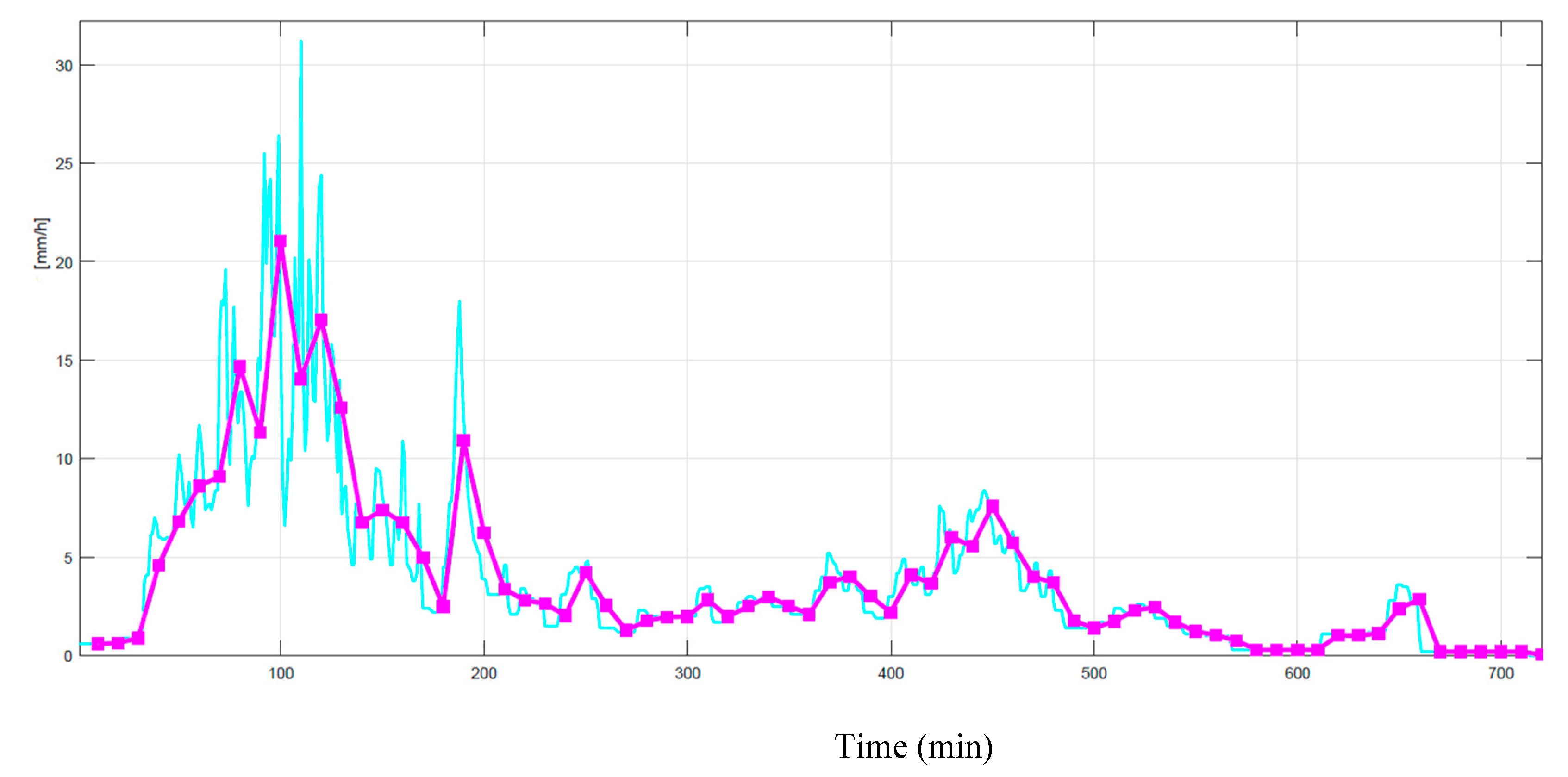
Figure 2.
Histograms of in the range mm/h of (left panel) and mm/h (right panel) of .
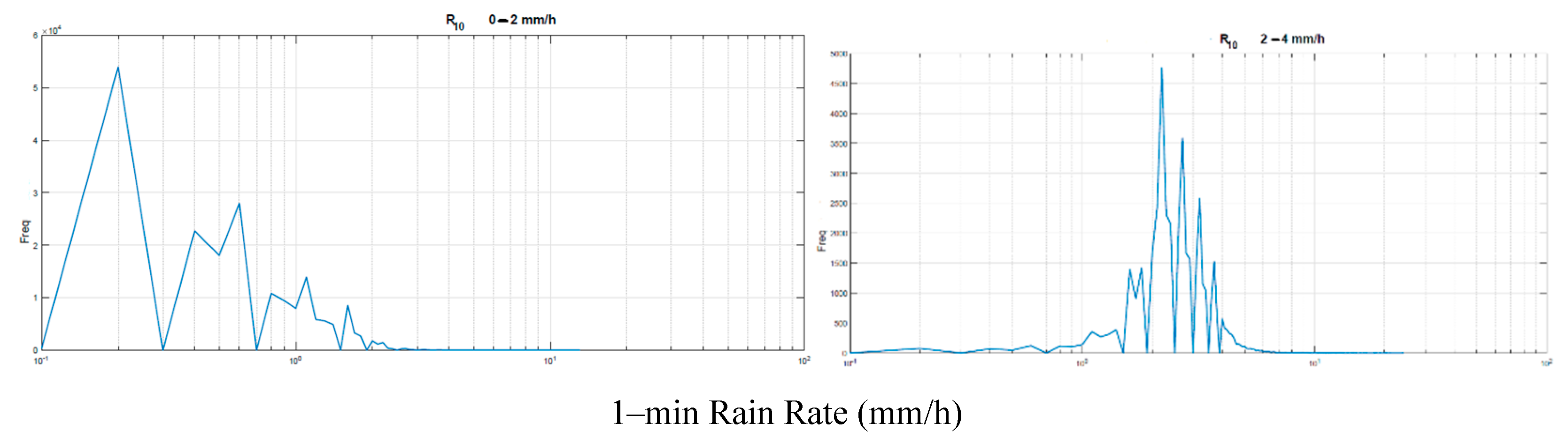
Figure 3.
Histograms of in the range mm/h of (left panel) and mm/h /right panel) of .

Figure 4.
Histograms of in the range mm/h of (left panel) and mm/h /right panel) of .
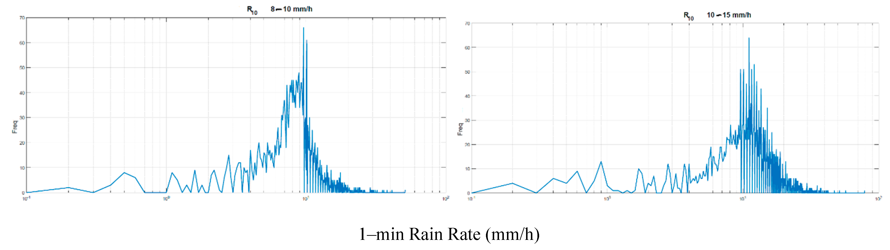
Figure 5.
Histograms of in the range mm/h of (left panel) and mm/h /right panel) of .
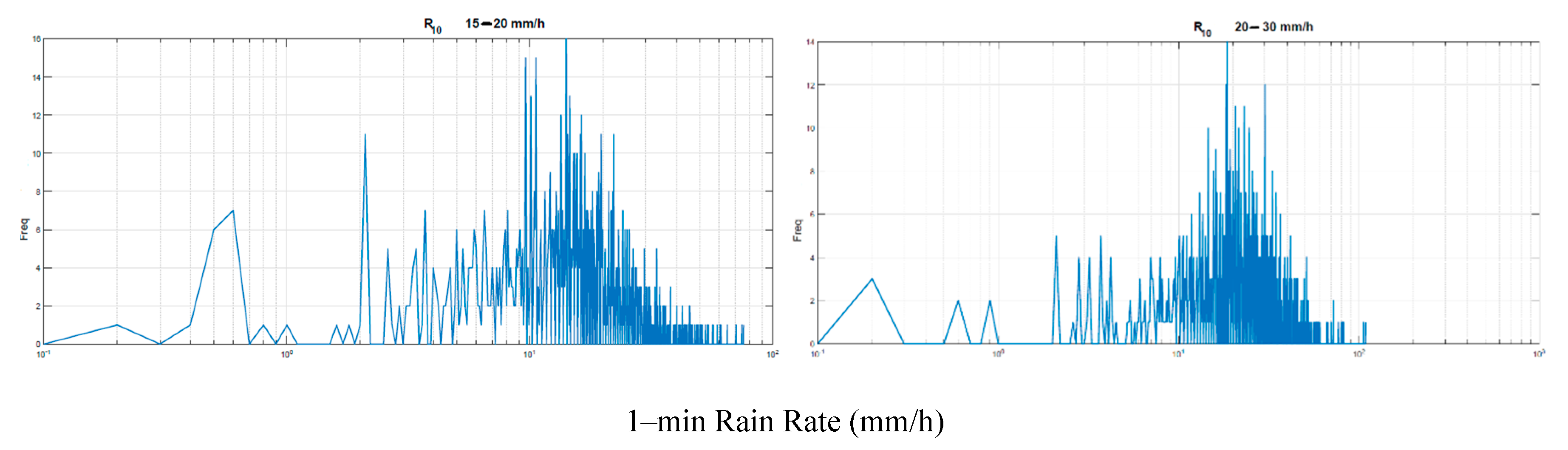
Figure 6.
Histograms of in the range mm/h of (left panel) and mm/h /right panel) of .
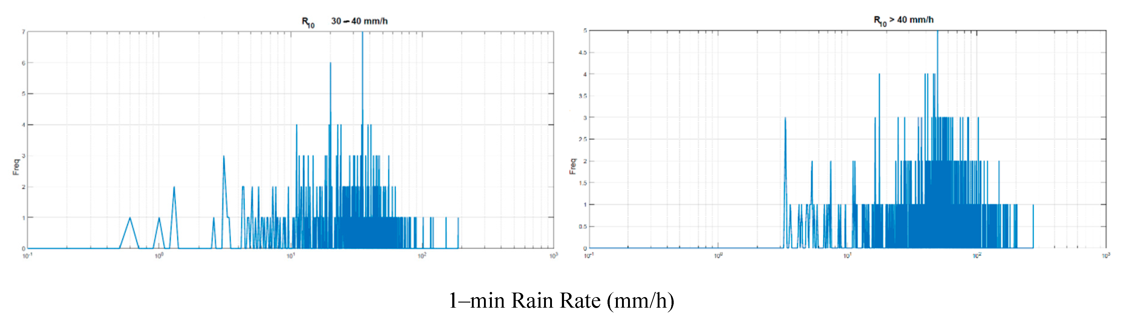
Figure 7.
Experimental (mm/h) (blue, original) and simulated (mm/h) time series (black, simul). Left: low intensity rain rate event; Right panel: high intensity rain–rate event. The 10–min quantity of water is conserved.
Figure 7.
Experimental (mm/h) (blue, original) and simulated (mm/h) time series (black, simul). Left: low intensity rain rate event; Right panel: high intensity rain–rate event. The 10–min quantity of water is conserved.
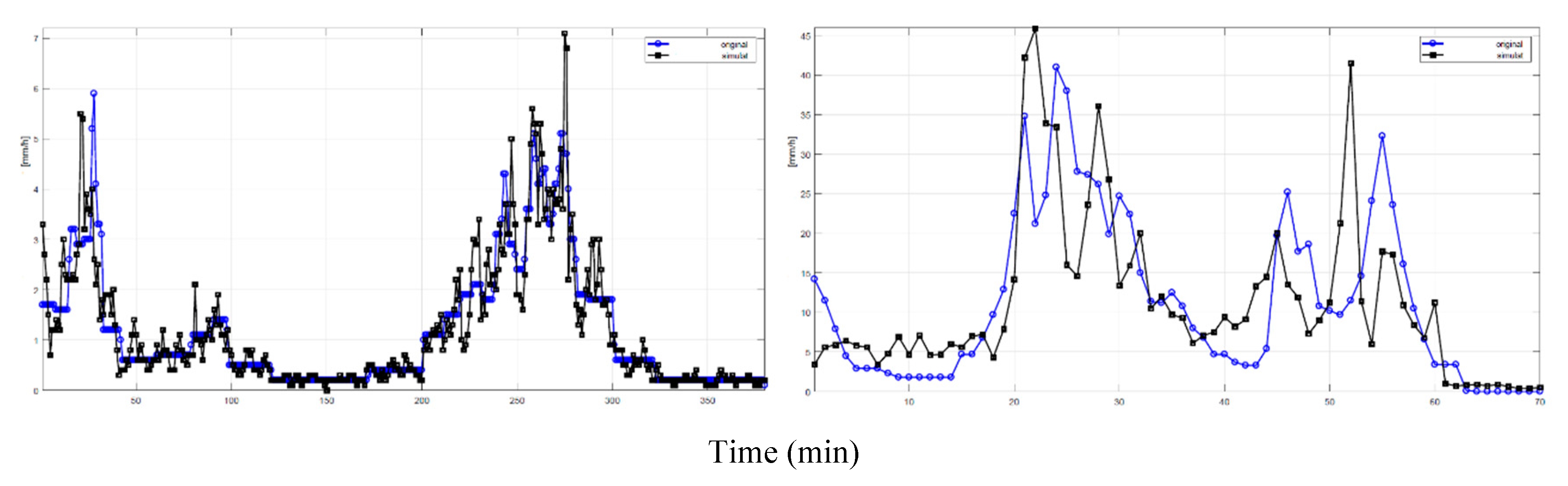
Figure 8.
Mean value (left panel, mm/h) and standard deviation (right panel, mm/h) of versus .
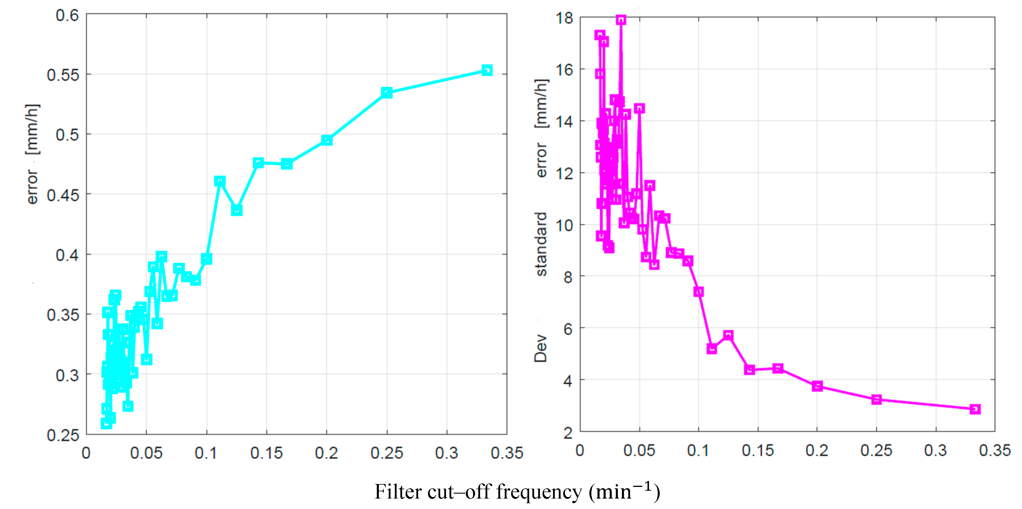
Figure 9.
Example of 1–min rain–rate time series, measured (blue line, original) and simulated (red line, gener), after filtering and water conservation. Left panel: a low rain rate event; Right panel: a high intensity rain rate event (see also Figure 7).
Figure 9.
Example of 1–min rain–rate time series, measured (blue line, original) and simulated (red line, gener), after filtering and water conservation. Left panel: a low rain rate event; Right panel: a high intensity rain rate event (see also Figure 7).
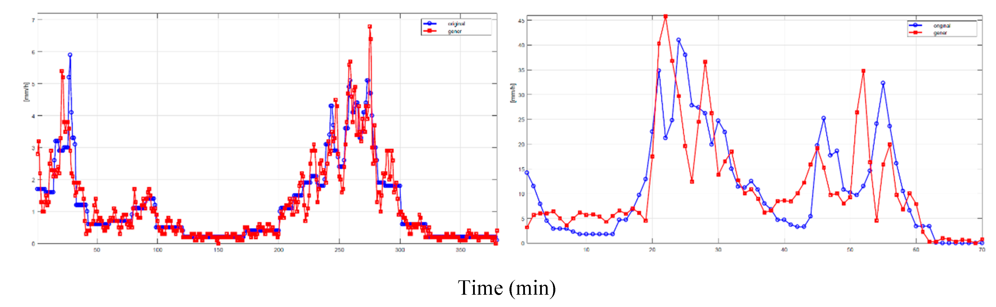
Figure 10.
Probability distrbution (PD) that the 1–min rain rate in abscissa is exceeded in the experimental data , blue line (original), and in the simulated 1–min data, , black line (simul).
Figure 10.
Probability distrbution (PD) that the 1–min rain rate in abscissa is exceeded in the experimental data , blue line (original), and in the simulated 1–min data, , black line (simul).
Table 1.
Geographical coordinates, altitude, number of years of continuous rain–rate time series measurements and wind speed at 700 mb (this latter parameter is necessary to apply the SST locally), at the indicated sites.
Table 1.
Geographical coordinates, altitude, number of years of continuous rain–rate time series measurements and wind speed at 700 mb (this latter parameter is necessary to apply the SST locally), at the indicated sites.
| Site | Latitude N (°) | Longitude E (°) | (m) | Continuous Observation Time (Years) |
~700 mb height () |
|---|---|---|---|---|---|
| Spino d’Adda (Italy) | 45.4 | 9.5 | 84 | 10 (1993–2002) | 10.6 |
| Gera Lario (Italy) | 46.2 | 9.4 | 210 | 5 (1978–1982) | 8.2 |
| Fucino (Italy) | 42.0 | 13.6 | 680 | 5 (1978–1982) | 10.4 |
| Madrid (Spain) | 40.4 | 356.3 | 630 | 9 (2006–2014) | 10.9 |
| Prague (Czech Republic) | 50.0 | 14.5 | 250 | 5 (1999–2003) | 12.6 |
| Tampa (Florida) | 28.1 | 277.6 | 50 | 4 (1995–1998) | 9.2 |
| White Sands (New Mexico) | 32.5 | 253.4 | 1463 | 5 (1994–1998) | 9.1 |
| Vancouver (British Columbia) | 49.2 | 236.8 | 80 | 3 (1995, 1996, 1998) | 12.4 |
Disclaimer/Publisher’s Note: The statements, opinions and data contained in all publications are solely those of the individual author(s) and contributor(s) and not of MDPI and/or the editor(s). MDPI and/or the editor(s) disclaim responsibility for any injury to people or property resulting from any ideas, methods, instructions or products referred to in the content. |
© 2024 by the authors. Licensee MDPI, Basel, Switzerland. This article is an open access article distributed under the terms and conditions of the Creative Commons Attribution (CC BY) license (http://creativecommons.org/licenses/by/4.0/).
Copyright: This open access article is published under a Creative Commons CC BY 4.0 license, which permit the free download, distribution, and reuse, provided that the author and preprint are cited in any reuse.


