Submitted:
20 November 2024
Posted:
26 November 2024
You are already at the latest version
Abstract
Gait analysis with step length estimation is essential not only for assessing an individual's health status, mobility, and balance but also for designing a pedestrian navigation system in infrastructure-less environments. This study presents an improved methodology for gait analysis and step length estimation (SLE) by applying a sequential neural network (SNN), a kind of artificial neural network, to sensor data collected from a foot-mounted inertial measurement unit. Our proposed methodology employs a Butterworth filter and normalization technique to smooth the sensor signals. Key gait-related features are then extracted and fed to the SNN, predicting step length without involving any user-specific parameter. The performance of our proposed SNN-based SLE method is evaluated and compared with our previously developed peak-valley detection-based SLE in terms of accuracy. Ten participants including both male and female (aged 24-50) took part in a walking experiment on a 60-meter linear path, walking under two modes – normal and fast. The accuracy results show that our new SNN-based SLE method achieves superior performance with accuracy exceeding 99.4% for each participant and demonstrates greater resilience to variations in user dynamics compared to our previously developed traditional Peak-Valley detection-based SLE method, confirming the proposed SNN-based approach as a superior solution.
Keywords:
gait
; step length
; sensor
; sequential neural network (SNN)
; accuracy
1. Introduction
Gait analysis and step length estimation are crucial for understanding human mobility offering valuable insights into an individual’s overall health, balance, and overall mobility [1,2,3]. Abnormal gait patterns often indicate various health conditions, including neurological disorders, musculoskeletal injuries, and cardiovascular diseases [4]. For instance, individuals with Parkinson’s disease typically display distinctive gait patterns, such as shuffling, freezing, and festination [5,6]. Similarly, athletes with injuries or musculoskeletal imbalances may exhibit altered gait patterns, potentially increasing their risk of further injury [7]. Beyond healthcare, gait analysis is also crucial in sports and robotics. In sports, gait analysis can help athletes optimize their performance, reduce the risk of injury, and enhance their overall efficiency. For example, analyzing the gait patterns of runners can help identify areas for improvement, such as stride length, cadence, and foot strike pattern [8]. In robotics, gait analysis plays a key role in the development of humanoid robots with human-like movement patterns, enabling them to navigate complex environments and interact with humans more effectively [9].
Among various methodologies available for gait analysis and estimation of gait features like step frequency, step length, etc., both optical motion capture systems and instrumented walkways require dedicated infrastructure and are thus limited to laboratory environments or clinical settings only [10]. Light-weight and low-cost inertial sensors, however, offer a viable alternative due to their applicability for use not only in clinical settings but also in home environments [11] as well as for different walking modes [12]. This has led to growing interest in long-term health monitoring of patients with spinal cord injury or neurological disorders outside of hospital or laboratory environments using inertial sensors attached to body parts such as the foot, thigh, waist, arm, etc. [13,14,15]. Step length estimation (SLE) also plays a crucial role in designing positioning and navigation systems using the dead reckoning method [16,17].
Traditional SLE methods utilize either some biomechanical [18,19,20,21] or model-based techniques [22,23,24] or rely on the empirical relationship between human gait and step/stride length [25,26]. Biomechanical models use the geometric relationship between step length and body segments whereas model-based techniques leverage the relationship between acceleration variance or step frequency and step length. However, these traditional methods depend heavily on the predetermined threshold values and require calibration of user-specific parameters, as their performance can be severely affected by the gait characteristics, walking mode, and the inertial sensor’s placement on the user. To address these limitations, machine learning models, including deep learning, have effectively been applied to estimate step/stride length and to design pedestrian navigation systems based on the processing of inertial sensor measurements [27,28,29,30,31,32,33,34].
In [27], Wang et al., combined several machine learning models, including k-nearest neighbor (KNN) [28], support-vector networks [29], decision trees [30], AdaBoost [31], LightGBM [32] and extreme gradient boost [33] for recognition of the smartphone carrying or holding mode and estimation of the user’s stride length. In this study, both time-domain and frequency-domain features of accelerometer and gyroscope data collected during movement were used for stride length estimation. To mitigate the negative effects of noisy sensor data and complex human movement on the performances of the pedestrian navigation system, Zhang et al. integrated an online sequential extreme learning machine (OS-ELM) [34] with the dead-reckoning method and used a sliding-window-based scheme to process sensor measurements [35]. Sui and Chang proposed a self-supervised learning scheme in [36] to train a convolutional neural network (CNN) model [37] using an unlabeled large dataset for user’s stride length estimation in walking and running modes. Other researchers, such as in [39], used stacked autoencoder [38] to make an SLE model adaptable to the user dynamicity and smartphone carrying modes, while Ping et al. employed Bidirectional Long Short-term Memory (LSTM) [40] for stride length estimation across various gait patterns and different walking modes [41]. A deep convolutional neural network [42] was used in [43] to generalize the step length estimation method across different walking speeds, while Wang et al. [44] used a combination of LSTM [40] and Denoising Autoencoder [45] to design a generalized SLE model for different movement patterns. In [46], Park et al. combined bidirectional LSTM with CNN to generalize their SLE technique to different users and motion patterns.
Despite the success of these SLE techniques, most require excessive training using large datasets to achieve reliable results across different users and motion patterns. The signal measurements collected from the inertial sensors are time series data whereas human gait patterns during walking are generally cyclic in nature. Based on these two observations, the sequential neural networks present a promising alternative. Sequential neural networks (SNNs) can be more effective in designing an SLE technique capable of generalizing across gait patterns and walking modes, even while trained using a small labeled dataset. Therefore, in this paper, we employ a sequential neural network (SNN) [47] to design a robust SLE technique that addresses the heterogeneity in human gait and walking modes, avoiding the need for training using a large dataset. Moreover, our proposed SLE model processes the sensor data from an inertial measurement unit (IMU) mounted on a single foot rather than relying on smartphone-integrated inertial sensors, reducing challenges related to smartphone carrying modes or placement positions. The proposed SLE model’s performance was evaluated with ten pedestrian participants across two walking modes and compared with our previously developed traditional peak-valley detection-based SLE method [48] to demonstrate its superior performance. The key contributions of our present work on the SLE method are as follows.
- In this study, we aim to develop a robust Step Length Estimation (SLE) technique by employing a sequential neural network due to its significant potential to address challenges arising from variations in human gait and waking modes, while also reducing the need for extensive training using large datasets.
- The proposed SLE model uses a single foot-mounted inertial measurement unit equipped with only a 3D accelerometer and a 3D gyroscope sensor.
- Performance analysis comparing the proposed SLE model to the previously developed traditional SLE method demonstrates that the SNN based proposed SLE model achieves superior performance results [48].
The paper is organized as follows. Section 2 describes the proposed methodology including the functional architecture of the adopted SNN model and the detailed specification of the IMU used. The performance evaluation of the proposed SLE method along with its comparative analysis is carried out in Section 3. Section 4 presents the concluding remarks and indicates further scope of research in the current domain.
2. Proposed Methodology
Our proposed SLE technique employs a Sequential Neural Network [47], which is a feedforward neural network well-suited for regression tasks. The SNN model used by our proposed methodology is trained using labeled input data collected from IMU sensors, i.e., a supervised learning approach, specifically, regression is used to predict the step length by our proposed methodology. The flow chart of our proposed SLE technique is shown in Figure 1. First, a detailed description of the functional architecture of the machine learning (ML) model adopted in this study and its constituent layers is presented in this Section. Then, the working procedure of the proposed SLE technique is described comprehensively.
2.1. Functional Architecture of Sequential Neural Network (SNN)
The visual representation of the architecture of the adopted ML model sequential neural network (SNN) is given in Figure 2. The connections in the diagram are congested because the number of nodes in the input and hidden layers is quite large (14 and 24 respectively). This creates a large number of possible connections between the layers. The diagram shows a fully connected neural network, meaning every node in the input layer connects to every node in the hidden layer. This leads to a large number of connections. The model’s architecture is designed to learn complex patterns in the input data and make accurate predictions of the step length.
2.1.1. Input Layer
A single input vector consisting of 14 features, which are derived from both acceleration and angular sensor measurements, are fed into the network via this layer and then propagates through the subsequent layers.
The 14 features are:
- i.
- Mean acceleration in the x-axis direction denoted by .
- ii.
- Mean acceleration in the y-axis direction denoted by .
- iii.
- Mean acceleration in the z-axis direction denoted by .
- iv.
- Mean angular velocity in the x-axis direction denoted by .
- v.
- Mean angular velocity in the y-axis direction denoted by .
- vi.
- Mean angular velocity in the z-axis direction denoted by .
- vii.
- Standard deviation of acceleration in the x-axis direction denoted by .
- viii.
- Standard deviation of acceleration in the y-axis direction denoted by .
- ix.
- Standard deviation of acceleration in the z-axis direction denoted by .
- x.
- Standard deviation of angular velocity in the x-axis direction denoted by .
- xi.
- Standard deviation of angular velocity in the y-axis direction denoted by .
- xii.
- Standard deviation of angular velocity in the z-axis direction denoted by .
- xiii.
- Stride duration () - it represents the duration of each stride segment in seconds and is calculated as follows.where is the number of samples in the current stride segment and is the sampling frequency of the data, which is the number of samples per second.
- xiv.
- Stride frequency () - it represents the frequency of the stride segment, i.e., the number of strides per second. It is the reciprocal of the stride duration and thus, is calculated as
The input vector is thus represented as follows.
2.1.2. Hidden Layer
The hidden layers are the core of the neural network, where complex representations of the input data are learned. The proposed model consists of two hidden layers, each with a specific configuration as given below.
Dense Layer 1: This layer consists of 64 neurons or nodes. Each node applies a Rectified Linear Unit (ReLU) activation function to the output of the previous layer. Such activation function is commonly used in the hidden layers because it is faster to compute than other activation functions like sigmoid or tanh and also allows the model to learn more complex relationships between inputs and outputs. The ReLU activation function is defined as , where x is input to the neuron. It returns 0 for when x is negative but the value of x itself in case x is positive or 0. The layer is mathematically represented by
where is the output of the ith neuron in the first hidden layer, f is the ReLU activation function, is the number of input features (14 in this case), is the weight connecting the jth input feature to the ith neuron in the first hidden layer, is the jth input feature and is the bias term for the ith neuron in the first hidden layer.
Dropout Layer 1: This layer applies a regularization technique that helps to prevent overfitting by randomly dropping out of the units during training. This forces the model to learn multiple representations of the data and improves its generalization capabilities.
Dense Layer 2: This layer consists of 32 neurons, each of which also applies the ReLU activation function. The layer further transforms the output of the previous layer, learning more complex patterns and relationships in the data. It is mathematically represented by
where is the output of ith neuron in the second hidden layer, f is the ReLU activation function, is the number of neurons in the first hidden layer (64 in this case), is the weight connecting the jth neuron in the first hidden layer to the ith neuron in the second hidden layer, is the output of the jth neuron in the first hidden layer and is the bias term for the ith neuron in the second hidden layer.
Dropout Layer 2: This layer applies the same dropout technique as before, randomly dropping out of the units during training, for the same reason as the Dropout Layer 1.
2.1.3. Output Layer
The output layer is a fully connected layer with a single neuron, which gives the predicted step length. It uses a linear activation function, where the target variable is continuous, making it suitable for the regression tasks. The layer is mathematically represented by
where y is the predicted step length, is the linear activation function, is the number of neurons in the second hidden layer (32 in this case), is the weight connecting the jth neuron in the second hidden layer to the output layer, is the output of the jth neuron in the second hidden layer and is the bias term for the output layer.
2.2. Working Procedure of Proposed SLE
The proposed step length estimation technique works in several steps as discussed below.
2.2.1. Step 1: Data Collection
The proposed SLE technique collects data from the IMU sensor mounted on a single foot as shown in Figure 3. The MPU6050 chip used in this study integrates a three-axis accelerometer and a three-axis gyroscope sensor and is also paired with an ESP32-WROOM-32D, enabling it to track the motion with high accuracy and low power consumption. The gyroscope sensor measures the angular velocity, while the accelerometer is used to measure the acceleration. The orientation of the sensor module’s coordinate system is configured in such a way that its Y-axis points towards the toe, the Z-axis remains normal to the foot’s surface, while the X-axis follows the right-hand rule. This configuration allows the Y-axis acceleration to capture the foot’s forward and backward movements, the Z-axis acceleration to detect the foot’s upward and downward movements, and the X-axis acceleration to sense the foot’s left and right movements.
2.2.2. Step 2: Data Preprocessing
A low-pass filter is used to remove the high-frequency noise from the collected sensor measurements followed by a normalization procedure to smooth out the signal.
Preprocessing via Low-pass Filter - A low-pass filter is a type of filter that allows low-frequency signals to pass through while attenuating high-frequency signals. The Butterworth low-pass filter [49], which is a type of recursive digital filter widely used in signal processing applications, is used in this study. The cutoff frequency and sampling frequency used to design the Butterworth low-pass filter are 10 Hz and 100 Hz respectively. The effects of applying the Butterworth filter on the Z-axis acceleration signal and X-axis gyroscope signal are shown in Figure 4 and Figure 5 respectively.
Preprocessing via Normalization – The filtered sensor measurements are normalized to smooth out the signal. The normalization process involves subtracting the mean of a set of data elements from the individual data element and then dividing the subtracted value by its standard deviation. The following equation defines the normalization process.
where B is a vector of time series data having n elements and represented as B = [, , ⋯, ], and are the mean and standard deviation of this time series data. The mean of B is computed as follows.
The standard deviation of B is calculated by the following equation.
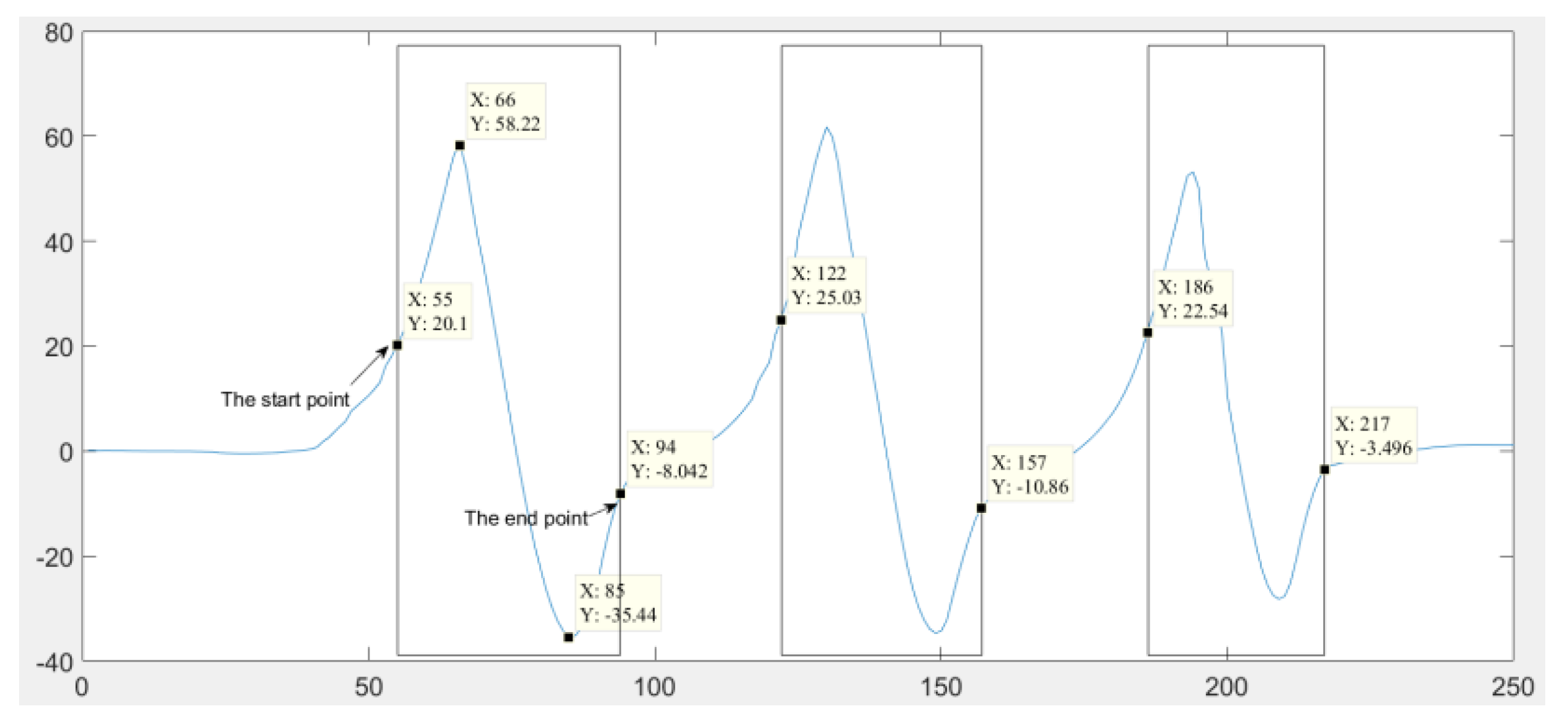
2.2.3. Step 3: Feature Extraction
The preprocessed data is segmented into strides, which are the basic units of movement. Each stride is a sequence of data points that corresponds to a single step. The features are then extracted by calculating the mean and standard deviation of the acceleration and angular velocity measurements obtained in each stride segment along with the stride duration and frequency as pointed out in subsection . The feature extraction process for acceleration and angular velocity signals are illustrated in Figure 8 and Figure 9 respectively. Considering S be the set of k () stride segments, where each segment ,where , is a sequence of multiple data points as shown in Figure 8 and 9. For each such segment , the mean and standard deviation are computed by applying equations 7 and 8 outlined in the previous subsection, whereas equations 1 and 2 given in subsection are used to derive the stride duration and stride frequency respectively. The feature vector for the stride segment (denoted as , ) is then constructed by concatenating the mean and standard deviation values of acceleration and angular velocity measurements corresponding to along with its stride duration and frequency. It is represented as follows.
The feature vectors for all stride segments are then collected into a matrix F, where each row corresponds to a single stride segment. The mathematical representation of feature matrix is given below.
The vector of observed step lengths, on the other hand, is represented by Y = [, , ⋯, ], based on the assumption that each stride segment represents one single step. Both the feature matrix and observed step length vector are split into the training and test datasets based on the rule that of the total dataset is included in the test dataset, whereas the remaining constitutes the training set.
2.2.4. Step 4: Model Training
The adopted SNN model is trained on the training dataset using a suitable optimization algorithm, such as Adam [50]. Adam is a stochastic gradient descent optimization algorithm, which adapts the learning rate for each parameter individually based on the magnitude of the gradient. The model is trained for a predetermined number of epochs with a certain batch size. The number of epochs indicates how many times the model is trained on the entire dataset, affecting how well the model converges to a good solution. A subset of the entire training dataset, on the other hand, constitutes a batch that is required to compute the gradient of the loss function and update the model’s parameters as well, thereby affecting the computational efficiency and accuracy of the model.
2.2.5. Step 5: Model Evaluation
The test dataset is used to evaluate the performances of the trained model in terms of mean squared error (MSE), which measures the average squared difference between the predicted and observed step lengths. MSE is calculated as follows.
where m is the number of data records in the test set, and denote the predicted and observed step length for the ith data record in the test set. Model evaluation is conducted to validate the trained model.
2.2.6. Step 6: Prediction of Step Length
Once the trained model is validated, it is then used to estimate the step length of a user based on a new input feature set.
3. Experimental Results and Discussions
The performance of our proposed SLE technique, based on the SNN model, was evaluated in terms of accuracy and compared with our previously proposed SLE method, which uses the Peak-Valley detection algorithm [48]. A 60-meter linear walking path was chosen for the experiment, with ten participants aged taking part in the study. A leave-one-out cross-validation approach was employed to assess the accuracy of our newly proposed SLE technique for each participant [51]. According to this approach, the gait features of each pedestrian used for step length prediction are included in the test set, while those of the remaining nine participants form the training set for the model. Additionally, the proposed method’s performance was tested under two different walking speeds—normal and fast—for each participant to demonstrate its effectiveness across varying walking modes.
The following equation calculates the accuracy of the proposed SLE method.
where and denote the step length estimated by the proposed method and the observed step length. At first, the experimental results obtained under normal walking and fast walking along with the basic body characteristics of each participant pedestrian are provided in Table 1 and Table 2 respectively. Then the accuracies of our newly proposed SNN-based SLE method and previously proposed peak-valley detection algorithm-based SLE method under two different walking modes, i.e., normal and fast are reported in Table 3 and Table 4 respectively.

Table 1.
Results of normal walking along with basic body characteristics of each participant pedestrian.
Table 1.
Results of normal walking along with basic body characteristics of each participant pedestrian.
| Participant | Walking | Average Step | Average | Height (m) | Weight (kg) | Gender |
|---|---|---|---|---|---|---|
| No. | Distance (m) | Length (m) | MSE loss | |||
| 1 | 60.2 | 0.599 | 0.03 | 1.706 | 80 | M |
| 2 | 60.2 | 0.593 | 0.03 | 1.706 | 67 | M |
| 3 | 60.4 | 0.667 | 0.06 | 1.803 | 75 | M |
| 4 | 60.1 | 0.628 | 0.04 | 1.803 | 57 | M |
| 5 | 59.8 | 0.609 | 0.07 | 1.706 | 58 | M |
| 6 | 60.3 | 0.591 | 0.06 | 1.706 | 60 | M |
| 7 | 60.4 | 0.612 | 0.04 | 1.625 | 56 | M |
| 8 | 60.6 | 0.552 | 0.03 | 1.574 | 40 | F |
| 9 | 59.9 | 0.562 | 0.08 | 1.752 | 70 | M |
| 10 | 60.8 | 0.588 | 0.02 | 1.706 | 70 | M |
Table 2.
Results of fast walking along with basic body characteristics of each participant pedestrian.
Table 2.
Results of fast walking along with basic body characteristics of each participant pedestrian.
| Participant | Walking | Average Step | Average | Height (m) | Weight (kg) | Gender |
|---|---|---|---|---|---|---|
| No. | Distance (m) | Length (m) | MSE loss | |||
| 1 | 60.4 | 0.703 | 0.07 | 1.706 | 80 | M |
| 2 | 60.7 | 0.666 | 0.08 | 1.706 | 67 | M |
| 3 | 60.3 | 0.701 | 0.08 | 1.803 | 75 | M |
| 4 | 60.9 | 0.738 | 0.04 | 1.803 | 57 | M |
| 5 | 60.4 | 0.679 | 0.07 | 1.706 | 58 | M |
| 6 | 60.8 | 0.612 | 0.06 | 1.706 | 60 | M |
| 7 | 60.7 | 0.674 | 0.08 | 1.625 | 56 | M |
| 8 | 59.8 | 0.601 | 0.07 | 1.574 | 40 | F |
| 9 | 59.6 | 0.672 | 0.08 | 1.752 | 70 | M |
| 10 | 60.7 | 0.702 | 0.09 | 1.706 | 70 | M |
Table 3.
Comparison of accuracy results under normal walking.
| Participant No. | Peak-Valley detection method (%) | SNN based method (%) |
|---|---|---|
| 1 | 92.03 | 99.61 |
| 2 | 92.27 | 99.52 |
| 3 | 98.29 | 99.76 |
| 4 | 97.44 | 99.55 |
| 5 | 96.54 | 99.78 |
| 6 | 93.83 | 99.68 |
| 7 | 98.31 | 99.46 |
| 8 | 88.35 | 99.78 |
| 9 | 93.68 | 99.52 |
| 10 | 98.29 | 99.67 |
Table 4.
Comparison of accuracy results under fast walking.
| Participant No. | Peak-Valley detection method (%) | SNN based method (%) |
|---|---|---|
| 1 | 96.62 | 99.52 |
| 2 | 96.4 | 99.55 |
| 3 | 93.43 | 99.46 |
| 4 | 98.37 | 99.61 |
| 5 | 97.6 | 99.52 |
| 6 | 92.77 | 99.56 |
| 7 | 97.79 | 99.67 |
| 8 | 93.94 | 99.61 |
| 9 | 96.3 | 99.46 |
| 10 | 94.78 | 99.52 |
The accuracy results reported in Table 3 and Table 4 show that the newly proposed step length estimator (Sequential neural network) boasts an impressive average accuracy exceeding , with a negligible average error rate of just . This remarkable achievement outperforms the traditional method based on the peak-valley detection algorithm, solidifying the proposed SNN-based approach as a superior solution. It is also evident from Table 3 and Table 4 that the SNN-based approach not only performs very well under two different walking modes compared to the traditional peak-valley detection-based approach but also the accuracy results of the former are not affected by user dynamicity. This happens because the newly proposed ML model-based method does not involve any user-specific parameter, thereby enhancing its resilience in its ability to adapt to the pedestrian’s dynamic pace changes, frequently occurring during walking, without compromising its accuracy.
4. Conclusions
This study demonstrates the effectiveness of an advanced ML-based step length estimator in delivering accurate step length estimates with minimal error. The proposed method is robust against noisy acceleration and angular velocity data from low-cost IMUs, achieving a low error rate of just over a 60-meter distance, as validated in experimental tests using a Sequential Neural Network (SNN).
Unlike traditional SLE methods that rely on peak-valley detection algorithms, our proposed SLE technique improves accuracy across different walking modes without requiring user-specific parameters or calibration. Using a straightforward, foot-mounted IMU with time data, this approach simplifies computations, enhancing performance overall. The accuracy and resilience of the SNN-based SLE method make it well-suited for applications such as monitoring the health status of patients with neurological disorders, and gait impairments, and also for the design of IMU sensor-based PDR systems tailored for indoor navigation.
Currently, the performance of the proposed SLE technique has been evaluated only on a linear path. Future research will extend this evaluation to non-linear paths with turns to assess its effectiveness in diverse walking environments. Additionally, we plan to validate the applicability of this method for monitoring gait health in patients with spinal cord injuries or neurological disorders by testing on a dataset that includes gait data from individuals with impaired movement as well as a wide range of ages and gait characteristics.
Author Contributions
Conceptualization, A.P. and P.S.; methodology, A.P.; software, A.P.; validation, A.P.; formal analysis, A.P., P.S., P.D. and N.R.; investigation, A.P.; resources, A.P. and P.S.; data curation, A.P.; writing—original draft preparation, A.P. and P.S.; writing—review and editing, P.D. and N.R.; visualization, A.P.; supervision, P.S.; project administration, A.P. and P.S.; All authors have read and agreed to the published version of the manuscript.
Funding
This research received no external funding.
Informed Consent Statement
Informed consent was obtained from all subjects involved in the study.
Acknowledgments
The authors gratefully acknowledge the facilities and support provided by the Director and all other staff members of the School of Mobile Computing and Communication, Jadavpur University, a Center of Excellence set up under the “University with potential for Excellence” Scheme of the UGC.
Conflicts of Interest
The authors declare no conflicts of interest.
References
- N. A. Abiad, Y. Kone, V. Renaudin and T. Robert, "Smartstep: A Robust STEP Detection Method Based on SMARTphone Inertial Signals Driven by Gait Learning," in IEEE Sensors Journal, vol. 22, no. 12, pp. 12288-12297, 15 June15, 2022. [CrossRef]
- Nahime Al Abiad, Enguerran Houdry, Carlos El Khoury, Valerie Renaudin, Thomas Robert, A method for calculating fall risk parameters from discrete stride time series regardless of sensor placement, Gait & Posture, Volume 111, 2024, Pages 182-184, ISSN 0966-6362. [CrossRef]
- Kelly A. Hawkins, Emily J. Fox, Janis J. Daly, Dorian K. Rose, Evangelos A. Christou, Theresa E. McGuirk, Dana M. Otzel, Katie A. Butera, Sudeshna A. Chatterjee, David J. Clark, Prefrontal over-activation during walking in people with mobility deficits: Interpretation and functional implications, Human Movement Science, Volume 59, 2018, Pages 46-55, ISSN 0167-9457. [CrossRef]
- Poleur M, Markati T, Servais L. The use of digital outcome measures in clinical trials in rare neurological diseases: a systematic literature review. Orphanet J Rare Dis. 2023 Aug 2;18(1):224. doi: 10.1186/s13023-023-02813-3. PMID: 37533072; PMCID: PMC10398976.
- S. V. Perumal and R. Sankar, "Gait monitoring system for patients with Parkinson’s disease using wearable sensors," 2016 IEEE Healthcare Innovation Point-Of-Care Technologies Conference (HI-POCT), Cancun, Mexico, 2016, pp. 21-24, doi: 10.1109/HIC.2016.7797687.
- Helena R. Gonçalves, Ana Rodrigues, Cristina P. Santos, Gait monitoring system for patients with Parkinson’s disease, Expert Systems with Applications, Volume 185, 2021, 115653, ISSN 0957-4174. [CrossRef]
- Hopin Lee, S. John Sullivan, Anthony G. Schneiders, The use of the dual-task paradigm in detecting gait performance deficits following a sports-related concussion: A systematic review and meta-analysis, Journal of Science and Medicine in Sport, Volume 16, Issue 1, 2013, Pages 2-7, ISSN 1440-2440. [CrossRef]
- Angkoon Phinyomark, Sean Osis, Blayne A. Hettinga, Reed Ferber, Kinematic gait patterns in healthy runners: A hierarchical cluster analysis, Journal of Biomechanics, Volume 48, Issue 14, 2015, Pages 3897-3904, ISSN 0021-9290. [CrossRef]
- Y. Tong, H. Liu and Z. Zhang, "Advancements in Humanoid Robots: A Comprehensive Review and Future Prospects," in IEEE/CAA Journal of Automatica Sinica, vol. 11, no. 2, pp. 301-328, February 2024, doi: 10.1109/JAS.2023.124140.
- Alexander Kvist, Fredrik Tinmark, Lucian Bezuidenhout, Mikael Reimeringer, David Moulaee Conradsson, Erika Franzén, Validation of algorithms for calculating spatiotemporal gait parameters during continuous turning using lumbar and foot mounted inertial measurement units, Journal of Biomechanics, Volume 162, 2024, 111907, ISSN 0021-9290.
- Guimarães, Vânia, Inês Sousa, and Miguel Velhote Correia. 2021. "A Deep Learning Approach for Foot Trajectory Estimation in Gait Analysis Using Inertial Sensors" Sensors 21, no. 22: 7517. [CrossRef]
- Hyang Jun Lee, Ji Sun Park, Hee Won Yang, Jeong Wook Shin, Ji Won Han, Ki Woong Kim, A normative study of the gait features measured by a wearable inertia sensor in a healthy old population, Gait & Posture, Volume 103, 2023, Pages 32-36, ISSN 0966-6362. [CrossRef]
- Rampp, A.; Barth, J.; Schülein, S.; Gaßmann, K.G.; Klucken, J.; Eskofier, B.M. Inertial Sensor-Based Stride Parameter Calculation From Gait Sequences in Geriatric Patients. IEEE Trans. Biomed. Eng. 2015, 62, 1089–1097.
- Chen, B.R.; Patel, S.; Buckley, T.; Rednic, R.; McClure, D.J.; Shih, L.; Tarsy, D.; Welsh, M.; Bonato, P. A web-based system for home monitoring of patients with Parkinson’s disease using wearable sensors. IEEE Trans. Biomed. Eng. 2011, 58, 831–836.
- Kluge, F.; Gaßner, H.; Hannink, J.; Pasluosta, C.; Klucken, J.; Eskofier, B.M. Towards Mobile Gait Analysis: Concurrent Validity and Test-Retest Reliability of an Inertial Measurement System for the Assessment of Spatio-Temporal Gait Parameters. Sensors 2017, 17, 1522.
- H. Xu, F. Meng, H. Liu, H. Shao and L. Sun, "An Adaptive Multi-Source Data Fusion Indoor Positioning Method Based on Collaborative Wi-Fi Fingerprinting and PDR Techniques," in IEEE Sensors Journal, doi: 10.1109/JSEN.2024.3443096.
- P. Sadhukhan et al., "IRT-SD-SLE: An Improved Real-Time Step Detection and Step Length Estimation Using Smartphone Accelerometer," in IEEE Sensors Journal, vol. 23, no. 24, pp. 30858-30868, 15 Dec.15, 2023, doi: 10.1109/JSEN.2023.3330097.
- Y. Jiang, Z. Li and J. Wang, "PTrack: Enhancing the Applicability of Pedestrian Tracking with Wearables," 2017 IEEE 37th International Conference on Distributed Computing Systems (ICDCS), Atlanta, GA, USA, 2017, pp. 2193-2199, doi: 10.1109/ICDCS.2017.111.
- J. -S. Hu, K. -C. Sun and C. -Y. Cheng, "A Kinematic Human-Walking Model for the Normal-Gait-Speed Estimation Using Tri-Axial Acceleration Signals at Waist Location," in IEEE Transactions on Biomedical Engineering, vol. 60, no. 8, pp. 2271-2279, Aug. 2013, doi: 10.1109/TBME.2013.2252345.
- D. Alvarez, R. C. Gonzalez, A. Lopez and J. C. Alvarez, "Comparison of Step Length Estimators from Weareable Accelerometer Devices," 2006 International Conference of the IEEE Engineering in Medicine and Biology Society, New York, NY, USA, 2006, pp. 5964-5967, doi: 10.1109/IEMBS.2006.259593.
- R. C. Gonzalez, D. Alvarez, A. M. Lopez and J. C. Alvarez, "Modified Pendulum Model for Mean Step Length Estimation," 2007 29th Annual International Conference of the IEEE Engineering in Medicine and Biology Society, Lyon, France, 2007, pp. 1371-1374, doi: 10.1109/IEMBS.2007.4352553.
- S. H. Shin, C. G. Park, J. W. Kim, H. S. Hong and J. M. Lee, "Adaptive Step Length Estimation Algorithm Using Low-Cost MEMS Inertial Sensors," 2007 IEEE Sensors Applications Symposium, San Diego, CA, USA, 2007, pp. 1-5, doi: 10.1109/SAS.2007.374406.
- Zhang, Honghui, Jinyi Zhang, Duo Zhou, Wei Wang, Jianyu Li, Feng Ran and Yuan Ji. “Axis-Exchanged Compensation and Gait Parameters Analysis for High Accuracy Indoor Pedestrian Dead Reckoning.” J. Sensors 2015 (2015): 915837:1-915837:13.
- Y. Yao, L. Pan, W. Fen, X. Xu, X. Liang and X. Xu, "A Robust Step Detection and Stride Length Estimation for Pedestrian Dead Reckoning Using a Smartphone," in IEEE Sensors Journal, vol. 20, no. 17, pp. 9685-9697, 1 Sept.1, 2020, doi: 10.1109/JSEN.2020.2989865.
- Kim, Jeong Won, Han Jin Jang, Dong-Hwan Hwang and Chansik Park. “A Step, Stride and Heading Determination for the Pedestrian Navigation System.” Journal of Global Positioning Systems 01 (2004): 0-0.
- I. Bylemans, M. Weyn and M. Klepal, "Mobile Phone-Based Displacement Estimation for Opportunistic Localisation Systems," 2009 Third International Conference on Mobile Ubiquitous Computing, Systems, Services and Technologies, Sliema, Malta, 2009, pp. 113-118, doi: 10.1109/UBICOMM.2009.23.
- Wang, Qu, Langlang Ye, Haiyong Luo, Aidong Men, Fang Zhao, and Changhai Ou. 2019. "Pedestrian Walking Distance Estimation Based on Smartphone Mode Recognition" Remote Sensing 11, no. 9: 1140. [CrossRef]
- T. Cover and P. Hart, "Nearest neighbor pattern classification," in IEEE Transactions on Information Theory, vol. 13, no. 1, pp. 21-27, January 1967, doi: 10.1109/TIT.1967.1053964.
- Cortes, C., Vapnik, V. Support-vector networks. Mach Learn 20, 273–297 (1995). [CrossRef]
- Quinlan, J.R. Induction of decision trees. Mach Learn 1, 81–106 (1986). [CrossRef]
- Freund, Yoav and Robert E. Schapire. “Experiments with a New Boosting Algorithm.” International Conference on Machine Learning (1996).
- Ke, Guolin, Qi Meng, Thomas Finley, Taifeng Wang, Wei Chen, Weidong Ma, Qiwei Ye and Tie-Yan Liu. “LightGBM: A Highly Efficient Gradient Boosting Decision Tree.” Neural Information Processing Systems (2017).
- Tianqi Chen and Carlos Guestrin. 2016. XGBoost: A Scalable Tree Boosting System. In Proceedings of the 22nd ACM SIGKDD International Conference on Knowledge Discovery and Data Mining (KDD ’16). Association for Computing Machinery, New York, NY, USA, 785–794. [CrossRef]
- N. -y. Liang, G. -b. Huang, P. Saratchandran and N. Sundararajan, "A Fast and Accurate Online Sequential Learning Algorithm for Feedforward Networks," in IEEE Transactions on Neural Networks, vol. 17, no. 6, pp. 1411-1423, Nov. 2006, doi: 10.1109/TNN.2006.880583.
- M. Zhang, Y. Wen, J. Chen, X. Yang, R. Gao and H. Zhao, "Pedestrian Dead-Reckoning Indoor Localization Based on OS-ELM," in IEEE Access, vol. 6, pp. 6116-6129, 2018, doi: 10.1109/ACCESS.2018.2791579.
- Ronneberger, O., Fischer, P., Brox, T. (2015). U-Net: Convolutional Networks for Biomedical Image Segmentation. In: Navab, N., Hornegger, J., Wells, W., Frangi, A. (eds) Medical Image Computing and Computer-Assisted Intervention – MICCAI 2015. MICCAI 2015. Lecture Notes in Computer Science, vol 9351. Springer, Cham. [CrossRef]
- J. -D. Sui and T. -S. Chang, "IMU Based Deep Stride Length Estimation With Self-Supervised Learning," in IEEE Sensors Journal, vol. 21, no. 6, pp. 7380-7387, 15 March 15, 2021, doi: 10.1109/JSEN.2021.3049523.
- Paper, D. (2021). Stacked Autoencoders. In: State-of-the-Art Deep Learning Models in TensorFlow. Apress, Berkeley, CA. [CrossRef]
- F. Gu, K. Khoshelham, C. Yu and J. Shang, "Accurate Step Length Estimation for Pedestrian Dead Reckoning Localization Using Stacked Autoencoders," in IEEE Transactions on Instrumentation and Measurement, vol. 68, no. 8, pp. 2705-2713, Aug. 2019, doi: 10.1109/TIM.2018.2871808.
- S. Hochreiter and J. Schmidhuber, "Long Short-Term Memory," in Neural Computation, vol. 9, no. 8, pp. 1735-1780, 15 Nov. 1997, doi: 10.1162/neco.1997.9.8.1735.
- Z. Ping, M. Zhidong, W. Pengyu and D. Zhihong, "Pedestrian Stride-Length Estimation Based on Bidirectional LSTM Network," 2020 Chinese Automation Congress (CAC), Shanghai, China, 2020, pp. 3358-3363, doi: 10.1109/CAC51589.2020.9327734.
- Alex Krizhevsky, Ilya Sutskever, and Geoffrey E. Hinton. 2017. ImageNet classification with deep convolutional neural networks. Commun. ACM 60, 6 (June 2017), 84–90. [CrossRef]
- H. Jin, I. Kang, G. Choi, D. D. Molinaro and A. J. Young, "Wearable Sensor-Based Step Length Estimation During Overground Locomotion Using a Deep Convolutional Neural Network," 2021 43rd Annual International Conference of the IEEE Engineering in Medicine & Biology Society (EMBC), Mexico, 2021, pp. 4897-4900, doi: 10.1109/EMBC46164.2021.9630060.
- Wang, Qu, Langlang Ye, Haiyong Luo, Aidong Men, Fang Zhao, and Yan Huang. 2019. "Pedestrian Stride-Length Estimation Based on LSTM and Denoising Autoencoders" Sensors 19, no. 4: 840. [CrossRef]
- Pascal Vincent, Hugo Larochelle, Yoshua Bengio, and Pierre-Antoine Manzagol. 2008. Extracting and composing robust features with denoising autoencoders. In Proceedings of the 25th international conference on Machine learning (ICML ’08). Association for Computing Machinery, New York, NY, USA, 1096–1103. [CrossRef]
- J. Park, J. Hong Lee and C. Gook Park, "Pedestrian Stride Length Estimation Based on Bidirectional LSTM and CNN Architecture," in IEEE Access, vol. 12, pp. 124718-124728, 2024, doi: 10.1109/ACCESS.2024.3454049.
- Sutskever, I., Vinyals, O., & Le, Q. V. (2014). Sequence to Sequence Learning with Neural Networks. Proceedings of the 27th International Conference on Neural Information Processing Systems (NIPS 2014), 3104-3112.
- Sadhukhan, Pampa, Bibhas Gayen, Chandreyee Chowdhury, Nandini Mukherjee, Xinheng Wang, and Pradip K. Das. "Human Gait Modeling with Step Length Estimation based on Single Foot Mounted Inertial Sensors." Available at SSRN 4830580 (2024), https://dx.doi.org/10.2139/ssrn.4830580.
- S. Butterworth, "On the Theory of Filter Amplifiers," Wireless Engineer, vol. 7, no. 10, pp. 536-541, 1930.
- T. Hastie, R. Tibshirani, and J. Friedman, The Elements of Statistical Learning, Springer, 2009.
- S. B. Kotsiantis. 2007. Supervised Machine Learning: A Review of Classification Techniques. In Proceedings of the 2007 conference on Emerging Artificial Intelligence Applications in Computer Engineering: Real Word AI Systems with Applications in eHealth, HCI, Information Retrieval and Pervasive Technologies. IOS Press, NLD, 3–24.
Figure 1.
Flow chart of Proposed SLE model.
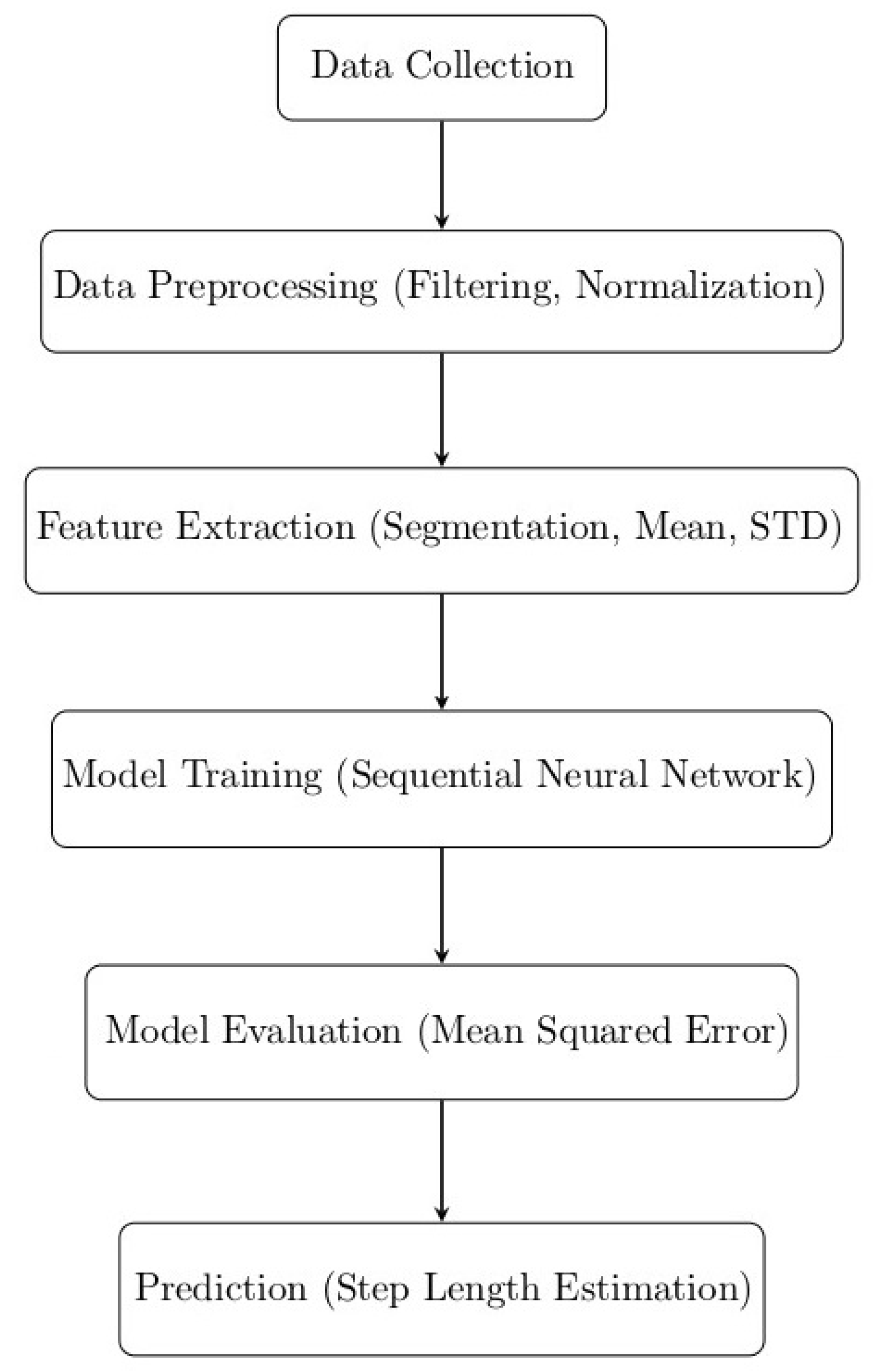
Figure 2.
Architecture of the Sequential Neural Network model.
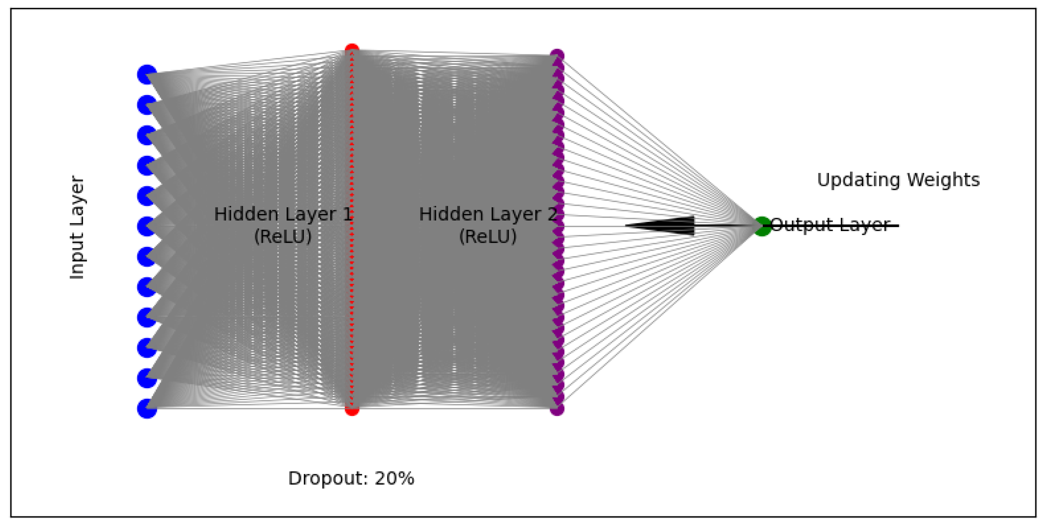
Figure 3.
Setup and Placement Position of IMU Sensor.
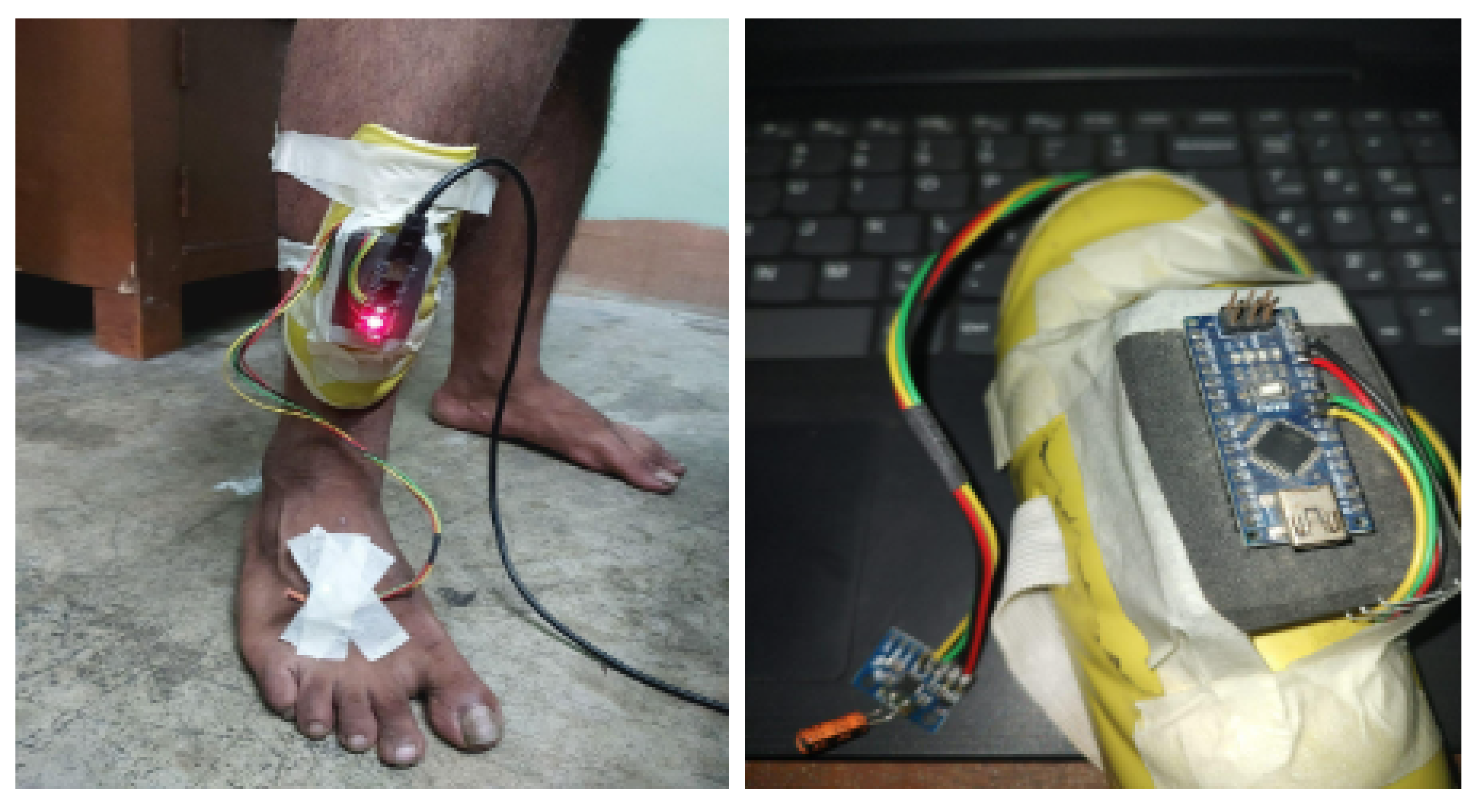
Figure 4.
Raw and Filtered Z-axis Acceleration Signal.
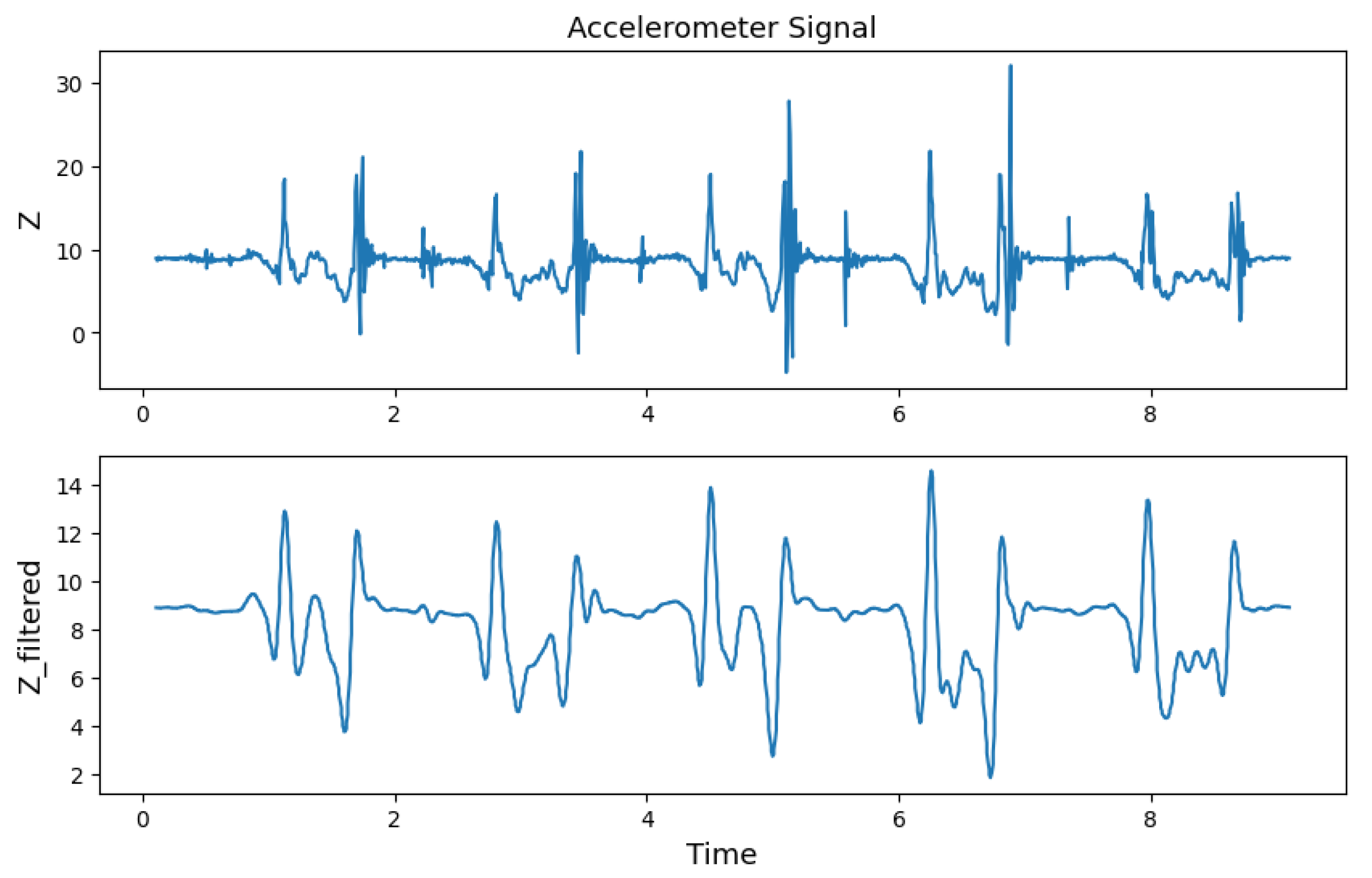
Figure 5.
Raw and Filtered Z-axis Acceleration Signal.
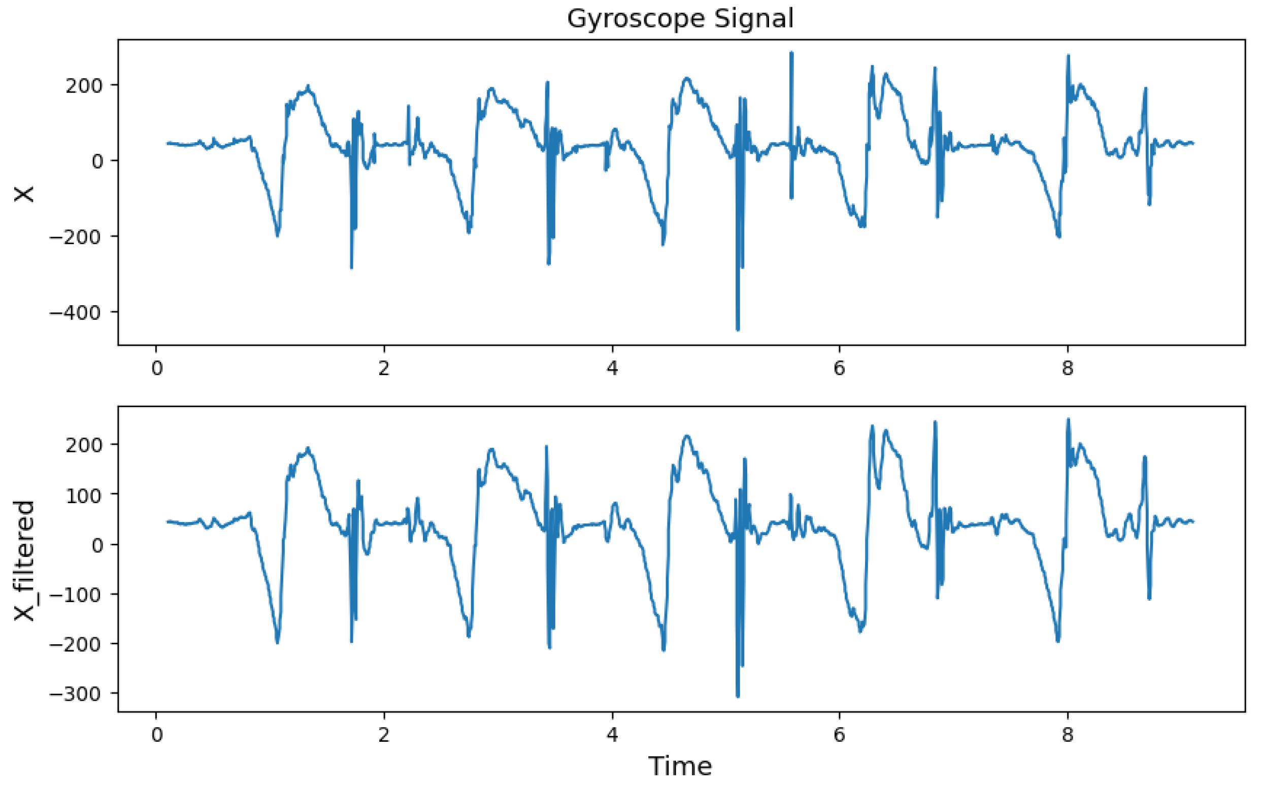
Figure 6.
Normalized Acceleration Signal.
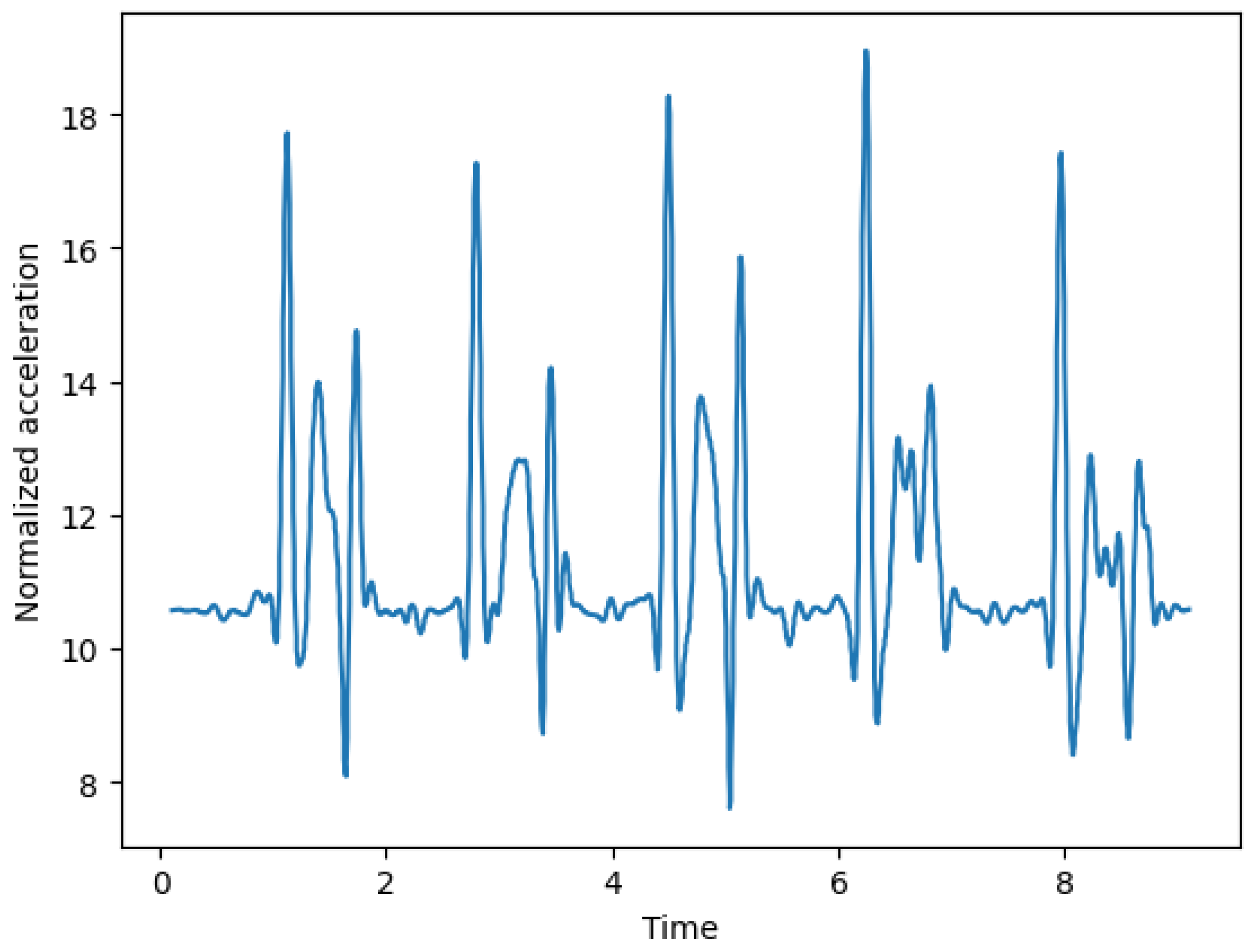
Figure 7.
Normalized Angular Velocity Signal.
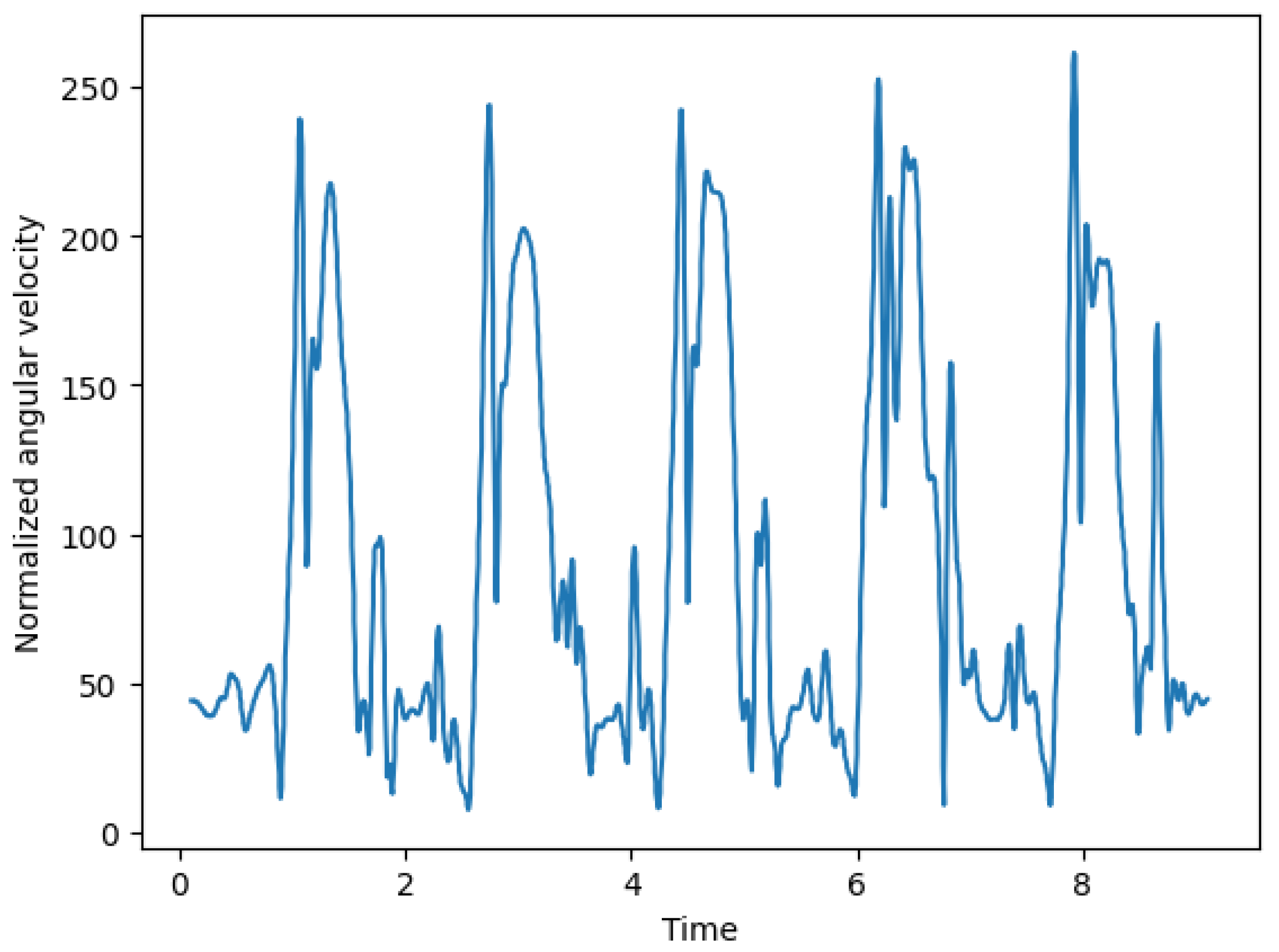
Figure 8.
Feature Extraction for Acceleration Signals.
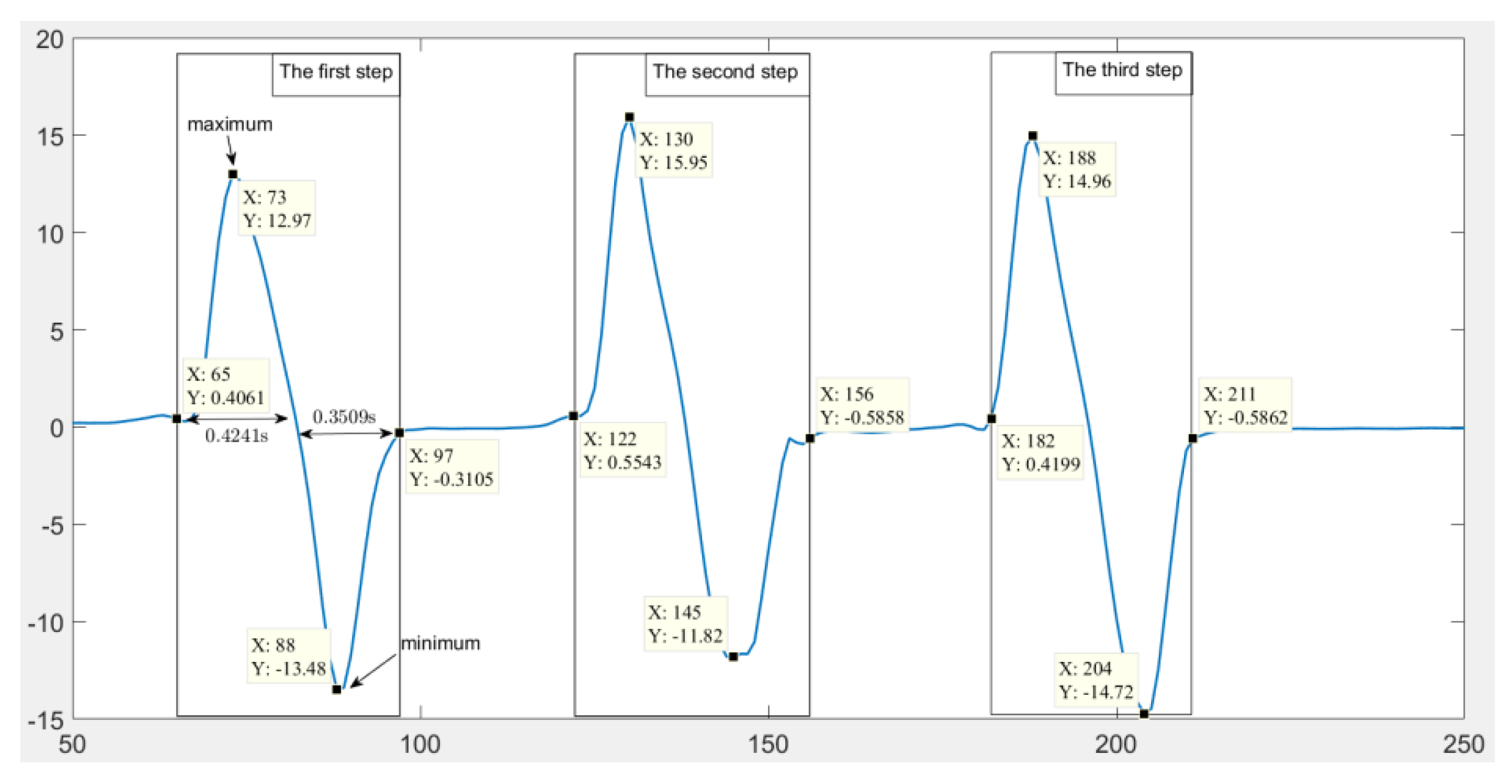
Figure 9.
Feature Extraction for Angular Velocity Signal.
Disclaimer/Publisher’s Note: The statements, opinions and data contained in all publications are solely those of the individual author(s) and contributor(s) and not of MDPI and/or the editor(s). MDPI and/or the editor(s) disclaim responsibility for any injury to people or property resulting from any ideas, methods, instructions or products referred to in the content. |
© 2024 by the authors. Licensee MDPI, Basel, Switzerland. This article is an open access article distributed under the terms and conditions of the Creative Commons Attribution (CC BY) license (http://creativecommons.org/licenses/by/4.0/).
Copyright: This open access article is published under a Creative Commons CC BY 4.0 license, which permit the free download, distribution, and reuse, provided that the author and preprint are cited in any reuse.


