Submitted:
24 November 2024
Posted:
25 November 2024
You are already at the latest version
Abstract
The capabilities of Physics-Informed Neural Networks (PINNs) to solve the Helmholtz equation in a simplified three-dimensional room are investigated. From a simulation point of view, it is interesting since room acoustic simulations often lack information from the applied absorbing material in the low-frequency range. This study extends previous findings toward modeling the 3D sound field with PINNs in an excitation case using DeepXDE with the backend PyTorch. The neural network is memory-efficiently optimized by mini-batch stochastic gradient descent with periodic resampling after 100 iterations. A detailed hyperparameter study is conducted regarding the network shape, activation functions, and deep learning backends (PyTorch, TensorFlow 1, TensorFlow 2). We address the computational challenges of realistic sound excitation in a confined area. The accuracy of the PINN results is assessed by a Finite Element Method (FEM) solution computed with openCFS. For distributed sources, it was shown that the PINNs converge to the solution, with deviations occurring in the range of a relative error of 0.28%. With feature engineering and including the dispersion relation of the wave into the neural network input via transformation, the trainable parameters were reduced to a fraction (around 5%) compared to the standard PINN formulation while yielding a higher accuracy of 1.54% compared to 1.99%.
Keywords:
PINNs
; FEM
; Helmholtz equation
; DeepXDE
; openCFS
; Acoustics
; Waves
; 3D
; PDE
; Room Acoustics
; Time-Harmonic Wave Field
; Absorber
1. Introduction
Today, there are persisting challenges in (room) acoustics simulations, with errors mainly arising from uncertain input parameters of used building material, resulting in high uncertainty of the used boundary conditions [1,2]. In particular, at low-frequent waves, the material parameters are off [3,4], hindering more accurate simulation results. These uncertain simulation input data underscore the importance of using algorithms that allow for the on-the-fly minimization of the model discrepancy with reality. As a selected algorithm, physics-informed neural networks (PINNs) can be used in forward mode (to predict the wave field) and inverse mode to infer material or boundary condition parameters with the use of data [3]. However, the computation of the time-harmonic acoustic wave field in large 3D geometries represents a challenge for current wave-based numerical and machine-learned methods [4,5]. The solutions to the Helmholtz equation in 3D are essential for understanding low-frequent room acoustic scenarios. The Finite Element Methods (FEM) analysis provides accurate results [4], but the extension to inverse parameters estimation is tedious compared to PINNs. PINNs show promising capabilities for that purpose, such that the interest in tailoring these algorithms to the accuracy of FEM became an interesting topic. So far, PINNs were used to solve the Helmholtz equation [6,7,8] only in 1D and 2D for acoustic simulations [3,9,10,11,12,13,14,15], ultra-sound application [16], electromagnetic waveguides [17,18] and aeroacoustics [19].
In extending the feasibility study [5], this paper performs a structured hyperparameter study of PINNs to solve the Helmholtz equation in 3D for a simple room acoustic simulation. We investigated the network size (concerning the results of [20]), the activation functions, and various backends, including PyTorch [21], TensorFlow 1 and 2 [22]. Compared to previous studies performed with well-behaving smooth excitation [9,20], we will analyze a realistic excitation scenario caused by a loudspeaker-like confined source. A first structured hyper-parameter study was conducted in [20], with hardly conclusive results on the network shape for the 3D setup as the outcome of hyper-parameter optimization using Gaussian processes-based Bayesian optimization. Furthermore, the loss metric, a point-wise l2 error measure, is suitable for training. However, it is questionable that a random distribution of evaluation points is computing a reliable error measure for the final neural network testing. In general, the Helmholtz equation is a linear partial differential equation, resulting in oscillatory fields, being a prototype for more complex solutions in fluid mechanics [23]. It was already observed and expected that the training deteriorates with increasing wave number due to the frequency-principle [24,25]. In addition to the standard neural network architectures, the locally adaptive activation functions with slope recovery [26] and the multi-scale Fourier feature network [27] are investigated for potentially improved neural network performance. The accuracy is evaluated by comparing the results on a structured evaluation grid with the FEM results and computing an L2 error norm during the hyperparameter study in 3D.
The article starts with Sec. 3 introducing the numerical examples of 3D room-like geometry with sound-hard boundary conditions, differential equation forcing including adaptive narrowing of the source by a sharpness parameter s, and material parameters. Section 4 presents the theoretical background of PINNs, experimental hyperparameter analysis, the multi-scale Fourier feature network [27], and the locally adaptive activation functions with slope recovery [26] in the context of acoustics. It is followed by the results section that presents the details of the investigations, the comparison to the FEM solution by error analysis, and the conclusions.
2. Room acoustic application
In the first step, we present the application example since it is essential to set up details on the PINN later. Previous studies have shown that the expected solution for the application example may significantly influence the network shape and capabilities used.
2.1. Case study setup
On a simple room-like 3D domain , the inhomogeneous Helmholtz equation
with homogeneous Neumann boundary conditions on is solved. In this equation, is the time-harmonic acoustic pressure, is the wavenumber, the angular frequency, c the speed of sound, g the forcing term, and is the Laplacian operator. A homogeneous Neumann boundary conditions model the room walls. The forcing consists of
with a source sharpness parameter s. As a follow-up to the previous 3D room acoustic examples [5], the source is modeled more realistically by a point source in the center of the room modeled for sufficiently small s. Throughout the study and in the hyperparameter study [20], the following physical parameter set
is varied.
2.2. Analytic solution and spatial frequency content
For , the forcing can be simplified to
This leads to an analytic solution of
that satisfies the forcing and the homogeneous Neumann boundary condition . In the current case, the solution is only real-valued ; however, in the general case, the solution is complex and may be treated by two independent networks, providing the independent solutions parts and . The spatial frequency of the solution is directly connected to the excited source by the linearity of the equation and is provided by the value of . For cases with , the solution wavenumber is primarily determined by . However, in the case of , the wave number content of the Gaussian envelope becomes important, which is determined by the Fourier transform of it
The frequency content governed by the Gaussian is sufficiently low for values of being smaller than two standard deviations. In our case, this condition reads or more specifically .
2.3. FEM reference simulation
A reference solution is computed using the FEM on the same setup with openCFS [28]. A fine mesh is used with approximately 40 degrees of freedom per wavelength satisfying the conditions of [29], resulting in 512000 elements of the computational domain. The mesh will deliver accurate results for and . For quadratic FEM basis functions, the mesh will provide accurate results for and [30].
3. Physics-informed neural networks for wave-based room acoustics
PINNs are fusing neural networks and complex partial differential equations (PDEs) for simulating physical systems using automated differentiation [31]. Figure 1 shows a multi-layer perceptron [32,33] network that can solve the Helmholtz Equation (1b) with appropriate boundary conditions.
Let be a L-layer-feed-forward neural network (FNN) (with -hidden neural network layers) to predict , with neurons in the ℓ-th layer . The output at a layer of a feed-forward neural network is calculated by repeated nonlinear activation-function weighted tensor products of (i) inputs and (ii) bias vector and weight matrix (e.g. in the ℓ-th layer by and , respectively), such that the FNN is recursively defined by
In the 3D case, the coordinates of one point are provided at the input layer. Defined by the neural network, the output prediction at the output layer L is calculated by
being a series of transformation functions. The network transformative operations can be summarized by a nonlinear operation depending on the trainable parameters, collecting all weights and biases , and the network input .
During training, will be learned by unlabeled training data , to approximate a continuous function mapping . The neural network operator approximates , regarding the minimal error described by the loss function . The loss will be minimized by
such that the weights and biases are adjusted to the converged ones . Within the study, we used the gradient-based optimization algorithm Adam [34] and the quasi-Newton method LBFGS [35]. The weights and biases are adapted iteratively by the gradient of to decrease , using backpropagation [36] and automatic differentiation [37]. A gradient descent algorithm updates the parameters such that
with representing the learning rate and i the epoch number.
The residual of the Helmholtz equation
with being the -norm integrated into the loss function to incorporate the inherent physical knowledge into the neural network training. It is evaluated at randomly sampled collocation points within the computational domain , forming the dataset comprises two sets, the points in the domain , of samples for the PDE residual and the points on the boundary , of samples for the boundary condition residual. The Neumann boundary condition residual is
which is sampled on the Neumann boundary forming the set . The total loss function can be described by
where and are weighting factors for the individual loss terms.
3.1. Initial Setup
The wavelength is selected to be . The PINN is set up using DeepXDE. Ten random collocation points per wavelength along each direction for training and 30 for validating are defined. A fully connected neural network uses a layer number layers and a layer width of neurons. A sinus activation function is used with Glorot uniform bias and weights initialization [38]. The loss term is defined in Equation (14), with , and . Figure 2a shows the exact solution of the acoustic pressure ( in a cut through the whole domain at . The network is trained over 30000 iterations by the ADAM optimizer with a learning rate of , resulting in a validation loss of 0.1248 (see Figure 2b). After 200 000 iterations by the ADAM optimizer, resulting in a validation loss of 0.0952, the relative error was 0.36% compared to the analytic solution. When changing the optimizer L-BFGS optimizer for 2000 iterations brings down the test loss to 0.0609 (see Figure 2c) and to 0.35%.
An explorative hyperparameter study was performed using the following parameter space
with , , , sin, ELU, GELU, ReLU, SELU, sigmoid, SiLU, swish, tanh}, PyTorch(P), TensorFlow 1 (T1), TensorFlow 2 (T2)}.
3.2. Locally adaptive activation functions
The locally adaptive activation function (LAAF) with slope recovery [26] is a method designed to improve the training speed and performance of deep and physics-informed neural networks. It introduces a scalable parameter, so-called activation slope (for layer ℓ and neuron i), to the activation function optimized during training. The locally adaptive activation function neural network (at the neuron level) is defined as
The output prediction at the output layer L is calculated by
being a series of transformation functions. The slope recovery term
encourages the network to increase the activation slope, leading to faster training. The loss function is extended to include the slope recovery term by
The analysis in [26] shows that LAAFs effectively multiply the gradients by conditioning matrices, accelerating convergence without explicitly calculating these matrices. Experiments demonstrated that LAAF works for deep neural networks in application for standardized datasets MNIST [39], Fashion-MNIST [40] and KMNIST [41], Semeion [42], SVHN [43], CIFAR [44]. Compared to fixed and global adaptive activations, neuron-wise LAAF exhibited faster training speeds when approximating a discontinuous function and, in combination with PINNs, the inverse problem of identifying the material coefficient of Poisson’s equation and Burgers equation in 2D. LAAF contributes to the overall challenge of reducing the number of iterations needed for convergence compared to the fixed activation function. This feature was tested with the backend TensorFlow 1 in DeepXDE and for the reliable hyperparameters with a network depth of , each layer consisting of 180 neurons, , the n of the DeepXDE implementation of layer-wise (a uniform for all neurons in the layer) LAAF is selected to be 2. The parameters selected were a good compromise for the standard PINN.
3.3. Multi-scale Fourier feature networks
The multi-scale Fourier feature architecture was proposed in [27] to address the spectral bias and low convergence rates observed in conventional PINN models [45]. The spectral bias expresses that the target function is first learned along the eigendirections connected to the larger eigenvalues of the neural tangent kernel and gradually the remaining components of smaller eigenvalues. Translated to conventional, fully connected neural networks, the eigenvalues are lowered by the increasing frequency of the corresponding eigenfunctions. As a result, the convergence rate of high-frequency components of is low [46,47]. This learning tendency is a significant challenge when dealing with multi-scale problems like localized acoustic sources featuring space-dependent high-frequency solution features. The challenge is addressed by embedding multiple Fourier features into the network to learn features across scales and to mitigate the spectral bias behavior. Firstly, the input coordinates are transformed using multiple Fourier feature mappings. The forward pass of M Fourier features with is defined by
where are preselected matrices with entries randomly sampled from a Gaussian distribution . The choice of values are additional hyperparameters that may be optimized, and typical values can be 1, 20, 50, 100 [27]. Overall, no new training parameters are introduced by this architecture compared to a standard fully connected neural network.
Figure 4.
Schematic representation of a PINN with multi-scale Fourier feature architecture.

3.4. Validation and testing procedure
The final physical validation (testing) of the PINN simulation was performed in pyCFS-data [48] using the relative -error measure on an evenly spaced evaluation sample (being an approximate of the relative -error)
where is the number of evaluation points, is the FEM reference pressure result and is the pressure result from the PINN. This error measure on a structured evaluation point sample is proportional to the error. The evenly spaced evaluation points of the FEM simulation have been used to evaluate the PINN prediction.
4. Results
The results are presented for the basic room application examples in 3D. Firstly, recent distinct hyperparameters are studied relying on optimization hypotheses in [20]. In [20], the authors presented a framework for automatically analyzing a set of hyperparameters in a Gaussian processes-based Bayesian optimization. Both a 2D and a 3D scenario were studied with a distributed force , with a very detailed description of the 2D case (Dirichlet problem), which in turn is not directly translatable to the 3D case (Neumann problem). The representativeness of the study shows limited training runs for the expensive training runs. The hyperparameter optimization study for the 3D case found an optimal configuration, learning rate , width of 207, depth of 10, with the sine activation function and a boundary weight term of 1 and the second best had a learning rate close to , width of 292, depth of 3, with the sine activation function and a boundary weight term of 19.1. The diversity of these two nearly optimal solutions expresses the challenge of training a network for this task. It was reported that for increased wave numbers, the performance of the PINNs was low in the 2D and 3D cases. Furthermore, by uniformly increasing the density of collocation points, the performance of the network prediction capability improved, suggesting that adaptive refinement may lead to further improvements. Upon those results [20], a structured hyperparameter exploration was conducted for the general 3D case with a finite source sharpness parameter s.
4.1. Sharpening the excitation source localization
In the next test, the source is modeled more by a gradually confined source in the center of the room modeled by (2) and illustrated in Figure 5a. The sharpness of the source can be tuned by the parameter s in the exponential. When sharpening the excitation of the source, additional spatial modes are immediately necessary to be modeled by the neural network and feature a multi-scale problem. As pointed out [27] and indicated by the modal description of a point source [49], it may be difficult for a standard fully-connected neural network to produce accurate results of the acoustic pressure Figure 5b.
The respective deviation
from the FEM pressure results to the case (analytical case ) is given in the Table 1 for the following s-parameters investigated. The relative deviations are important since any meaningful learned solution to that problem may at least have an error below that level.
The lowest level of was chosen to respect the frequency considerations for accurate FEM solutions of the source concerning the FEM mesh. The standard network with hyperparameters PyTorch}, a learning rate of and after 200 000 iterations motivated by [5,27] resulted in an error of for , resulted in an error of for , resulted in an error of for , and for . In conclusion, the standard networks were not able to learn a solution that was close to the FEM solution as soon as the source was sharpened.
4.2. Explorative hyperparameter study for
Compared to the previous studies conducted for , the study investigates the networks’ capability of calculating the results for a slightly distorted field based on . In that case, the amplitudes of the solution are marginally higher due to reflections at the sound-hard walls than for the simple example .
A relative error less than the relative deviations from the case indicates that the network has learned a meaningful description of the field. The configuration performed best in Table 2 and for the first cohort (separated by rules in the table). This trend was observable for all hyperparameter tests provided in Table 2. In the second and third cohorts, a combination of switching the optimizer during the training was tested, and the effect of this on performance was examined.
Interestingly, when using , the PDE and the BC loss were initially of the same level and caused an excellent prediction when combining it with the LBFGS optimizer to further iterate on the network parameters (orange row in Table 2). In the final two cohorts, the boundary condition weights were tested.
In a subsequent study, the network width was tested, and its influence on the performance (Table 3). As expected, narrow networks performed poorly, and until 60 neurons of layer width, nearly no convergence to the FEM results was obtained. In conclusion, the layer width between 120 and 240 gave acceptable results for this case. The accuracy was in the bounds for all tested backends, with a somewhat superior performance of TensorFlow 1 leading to an error below 2%.
Following up on the layer number and width study (Table 4), the activation functions were tested sin, ELU, GELU, ReLU, SELU, sigmoid, SiLU, swish, tanh}. From the shape of the solution, oscillating around the zero, the functions ELU, GELU, ReLU, SELU, sigmoid, and SiLU potentially performed poor, which was confirmed in the tests; none of the networks using those activation functions reached converged results with error less than 50%. The sinus function performed best; the swish and tanh activation reached similar errors, which were already quite large.
To improve the convergence and accuracy of the results, the layer-wise LAAF is a promising approach with its additional degrees of freedom and more rapid adjustments in learning the function approximation. For the layer-wise LAAF, only a few new parameters were added to the network, the number of hidden layers. Overall, the performance of the LAAF was superior compared to other n parameters tested.
As a conclusion for this experimental hyperparameter study, we found that a layer number of 2 or 3 will be a reasonable choice for this network. The layer width of around 120-240 is preferable, with the sin activation function and switching the training from initial Adams iterations of about 100 000 with a boundary weight of 5 and then switching to L-BFGS using a boundary weight of 50. The LAAF PINN structure did not further enhance the performance and accuracy. Overall, the accuracy compared to the FEM seems limited already for this relatively distributed source at . As a next step, we are investigating the potential of adaptive refinement in terms of the network accuracy and if further data is needed for that application example to improve for and the cases of .
4.3. Adaptive refinement of training set
In a subsequent step, the pre-trained standard network architecture with hyperparameters PyTorch}, a learning rate of and after 200 000 iterations are used for adaptive fine-tuning of the model. The idea that adaptive refinement may improve the results came up by looking at Figure 6a and the overlaid black dots, which seemed to be distributed nicely but were relatively few points compared to a FEM mesh. The adaptive refinement procedure worked in the following steps; in the first data refinement step, , the domain was sampled uniformly for a new dataset . At these data points the residual of the loss (14) was evaluated and the arbitrary choice of 150 data points with the most significant residual was added to . After the uniform refinement step, another 25 data refinement steps with random data point sampling were added to the training data points. In each refinement cycle, 1000 iterations of the optimizer were carried out, with early stopping activated.
The relative error results (21) for the case present a reduction of the error from 0.35% to 0.33% in the first refinement stage and then another reduction to 0.28% after the whole procedure of adaptive refinement. This reduction of 0.07% points is an improvement of the network’s prediction accuracy by 20%. Figure 6a illustrates the pressure field predicted by the PINN in the evaluation plane () with a colormap representing the pressure magnitude. Overlaid black dots highlight the training points close to the evaluation plane. Overlaid red dots highlight the training points the adaptive refinement procedure added and indicate regions where the training error was high before the refinement. Figure 6b shows the pressure field predicted by the PINN compared to the analytic solution in the evaluation line (). Notably, the graphs do coincide qualitatively.
In the case of , the relative error results (21) present a reduction of the error from 2.38% to 1.41% in the first refinement stage and then and a relative increase to 1.78% after the whole procedure of adaptive refinement. Overall, the improvement was 25.2% with an improvement of 40.8% after the first refinement stage.
Figure 7 summarizes the adaptive refinement procedure and the added data points to the training set. Notably, more training points were added in central areas of the plot compared to the case of . Interestingly, in Figure 7b, the pressure results of the PINN are good at approximating the amplitude reduction close to the boundary for and . However, deviations occur in the intermediate range, where and .
Since the relative errors were significant for the cases of , we expect some improvements to the results from the adaptive refinement procedure. For example, the case is discussed, featuring an error of nearly 100%. In the adaptive refinement step, the error was reduced to about 70%, but still in the range of being unacceptable compared to the FEM results.
Due to the adaptive refinement, the point distribution showed a remarkably uniform behavior, and the loss is significant in a large area (see Figure 8). Furthermore, a strong cluster of points close to the source location at is visible and was expected. Overall, the amplitude of the FEM result of was not captured by the neural network solution. Based on Figure 8, the qualitative behavior of the PINN solution looks fair. With further improvement and studies on the network’s capabilities, the solution to the forward problem in room acoustics is within reach.
4.4. Multi-scale Fourier feature networks
The pre-knowledge of spatial scales in the system is strongly driven by the behavior of the wave and the emissions coinciding with the wavelength . Furthermore, it is expected that based on the sharpening of the force, the spatial frequency content gets more dispersed over the wave number and can lead to approximation difficulties using a modal field [49]. This was formally shown in the Section 2.2. We selected an architecture with hyperparameters TensorFlow 1}, a learning rate of and after 200 000 the errors were evaluated. The Fourier features were selected from a normal distribution with a standard deviation of and , which is in the range of the wavelength based on the selected wave number. In the case of , the relative error (21) with 1.5% was in the range of the ordinary feed-forward network with the same number of trainable parameters. This was also observed for the case with an error of 5.4%. We observed no convergence for all the repeated test runs for , which was unexpected. In a second test, the activation function of the network neurons was altered to tanh to avoid the possible poor performance of a combination of Fourier feature inputs and sinus activation functions. Similarly, the relative error measure was 1.4%, 5.6%, and no convergence for , for and , respectively.
Overall, the multi-scale Fourier feature networks performed similarly to the standard model. A possible explanation is based on the exact linearization of the input-output relation due to the wave’s dispersion relation [50]. In the precise form, the cosine and sine transformation result for the various FEM results in the following linear relations illustrated in Figure 9.
Furthermore, the cosine Figure 9a analytically fulfills the boundary condition of sound hard walls. However, for a slightly shifted wavelength (by 10%), one can identify that the cosine and sine both transform into ellipses, making it comparably hard to solve the wave equation and estimate the solution. As soon as there is a deviation in the wave number, inherently present in the multi-scale network by the random draw of the Fourier features, it is fundamentally hard for the network architecture to find the solution of the wave equation. These facts motivate deterministic feature engineering [51,52] for the spatial coordinates to satisfy the dispersion relation of the wave.
4.5. Input feature generation
The ordinary input is now transformed before feeding it into the input by , with m such that the wave number frequency relation is respected. The transform is motivated by Green’s function of the waves in a box modeled by a complete orthonormal solution basis as a product of solutions for each Cartesian coordinate:
Note that an additive ansatz would fail and not reduce the complexity of the PINN problem. We selected an architecture with hyperparameters PyTorch}, a learning rate of and after 20 000 iterations the errors were evaluated. In doing so, the following errors were reached %, 1.54%, and 69% , , and , respectively. This significantly improves the other network structures by ingraining expert knowledge. For , the errors are in the range of the FEM method, and training took a few seconds, which is even faster than the FEM solution. We obtained no convergence of the amplitudes in the case of and . In Figure 10, the pressure prediction of the PINN compared to the analytic or FEM results is illustrated.
5. Conclusion
This study demonstrates the feasibility of using PINNs (DeepXDE) to model 3D sound fields governed by the Helmholtz equation in a confined room. The prediction accuracy was assessed by a reference FEM simulation in openCFS. Three different network architectures and feature engineering were used to improve the pressure field prediction. The most significant improvement was reached by ingraining the characteristics of the Green’s function based on modal expansion via feature into the PINN. Before reaching this model, a detailed hyperparameter study highlights the importance of optimizing network shape and activation functions to improve the prediction capability for a simple, fully connected neural network architecture. The variation of the deep learning backend showed slight improvements in the prediction accuracy. Due to the high computational demand and focus on the prediction accuracy in terms of a relative L2 error, no comparison of network architectures concerning the computational speed was carried out by intention. The fully connected layer-based PINN approach successfully converges to accurate solutions, as validated by FEM results, with relative errors as low as 0.28% for distributed sources. Adaptive refinement improved the prediction accuracy. It was shown that with the use of random Fourier features, no significant improvement was gained. Also, the network structure of layer-wise locally adaptive activation functions with slope recovery did not show improvements in prediction capability. However, the neuron-wise algorithm, introducing more additional degrees of freedom, might be a promising alternative for future evaluations. By incorporating Green’s function features equivalent to embedding the wave’s dispersion relation, a significantly reduced number of trainable parameters reached 5%, while improving accuracy by three orders of magnitude. This work underscores the potential of PINNs as a memory-efficient alternative to traditional methods for low-frequency room acoustic simulations, addressing challenges related to material absorption properties and complex excitation scenarios. As a result, future work could address the challenges of modeling confined source regions.
Funding
This scientific work was significantly supported by the COMET project ECHODA (Energy Efficient Cooling and Heating of Domestic Appliances). ECHODA is funded within the framework of COMET - Competence Centers for Excellent Technologies by BMK, BMAW, the province of Styria as well as SFG. The COMET programme is managed by FFG.
Institutional Review Board Statement
Not applicable
Data Availability Statement
The simulation data presented in this study are available on request from the author.
Conflicts of Interest
The authors declare no conflicts of interest.
References
- Jeong, C.H. Room acoustic simulation and virtual reality-Technological trends, challenges, and opportunities. J. Swed. Acoust. Soc.(Ljudbladet) 2022, 1, 27–30.
- Vorländer, M. Computer simulations in room acoustics: Concepts and uncertainties. The Journal of the Acoustical Society of America 2013, 133, 1203–1213. [CrossRef]
- Schmid, J.D.; Bauerschmidt, P.; Gurbuz, C.; Eser, M.; Marburg, S. Physics-informed neural networks for acoustic boundary admittance estimation. Mechanical Systems and Signal Processing 2024, 215, 111405. [CrossRef]
- Kraxberger, F.; Kurz, E.; Weselak, W.; Kubin, G.; Kaltenbacher, M.; Schoder, S. A Validated Finite Element Model for Room Acoustic Treatments with Edge Absorbers. Acta Acustica 2023, 7, 1–19. [CrossRef]
- Schoder, S.; Kraxberger, F. Feasibility study on solving the Helmholtz equation in 3D with PINNs. arXiv preprint arXiv:2403.06623 2024.
- Lu, L.; Pestourie, R.; Yao, W.; Wang, Z.; Verdugo, F.; Johnson, S.G. Physics-informed neural networks with hard constraints for inverse design. SIAM Journal on Scientific Computing 2021, 43, B1105–B1132. [CrossRef]
- Chen, Y.; Lu, L.; Karniadakis, G.E.; Dal Negro, L. Physics-informed neural networks for inverse problems in nano-optics and metamaterials. Optics express 2020, 28, 11618–11633. [CrossRef]
- Cuomo, S.; Di Cola, V.S.; Giampaolo, F.; Rozza, G.; Raissi, M.; Piccialli, F. Scientific machine learning through physics–informed neural networks: Where we are and what’s next. Journal of Scientific Computing 2022, 92, 88. [CrossRef]
- Lu, L.; Meng, X.; Mao, Z.; Karniadakis, G.E. DeepXDE: A deep learning library for solving differential equations. SIAM Review 2021, 63, 208–228. [CrossRef]
- Song, C.; Alkhalifah, T.; Waheed, U.B. Solving the frequency-domain acoustic VTI wave equation using physics-informed neural networks. Geophysical Journal International 2021, 225, 846–859. [CrossRef]
- Escapil-Inchauspé, P.; Ruz, G.A. Hyper-parameter tuning of physics-informed neural networks: Application to Helmholtz problems. Neurocomputing 2023, 561, 126826. [CrossRef]
- Gladstone, R.J.; Nabian, M.A.; Meidani, H. FO-PINNs: A First-Order formulation for Physics Informed Neural Networks. Arxiv Preprint 2022. [CrossRef]
- Wu, Y.; Aghamiry, H.S.; Operto, S.; Ma, J. Helmholtz-equation solution in nonsmooth media by a physics-informed neural network incorporating quadratic terms and a perfectly matching layer condition. Geophysics 2023, 88, T185–T202. [CrossRef]
- Jagtap, A.D.; Shin, Y.; Kawaguchi, K.; Karniadakis, G.E. Deep Kronecker neural networks: A general framework for neural networks with adaptive activation functions. Neurocomputing 2022, 468, 165–180. [CrossRef]
- Rasht-Behesht, M.; Huber, C.; Shukla, K.; Karniadakis, G.E. Physics-informed neural networks (PINNs) for wave propagation and full waveform inversions. Journal of Geophysical Research: Solid Earth 2022, 127, e2021JB023120. [CrossRef]
- Shukla, K.; Di Leoni, P.C.; Blackshire, J.; Sparkman, D.; Karniadakis, G.E. Physics-informed neural network for ultrasound nondestructive quantification of surface breaking cracks. Journal of Nondestructive Evaluation 2020, 39, 1–20. [CrossRef]
- Khan, M.R.; Zekios, C.L.; Bhardwaj, S.; Georgakopoulos, S.V. A Physics-Informed Neural Network-Based Waveguide Eigenanalysis. IEEE Access 2024. [CrossRef]
- Pan, Y.Q.; Wang, R.; Wang, B.Z. Physics-informed neural networks with embedded analytical models: Inverse design of multilayer dielectric-loaded rectangular waveguide devices. IEEE Transactions on Microwave Theory and Techniques 2023. [CrossRef]
- Schoder, S.; Museljic, E.; Kraxberger, F.; Wurzinger, A. Post-processing subsonic flows using physics-informed neural networks. In Proceedings of the Proceedings of 2023 AIAA Aviation Forum, AIAA, San Diego, 2023; pp. 1–8. [CrossRef]
- Escapil-Inchauspé, P.; Ruz, G.A. Hyper-parameter tuning of physics-informed neural networks: Application to Helmholtz problems. Neurocomputing 2023, 561, 126826. [CrossRef]
- Paszke, A.; Gross, S.; Massa, F.; Lerer, A.; Bradbury, J.; Chanan, G.; Killeen, T.; Lin, Z.; Gimelshein, N.; Antiga, L.; et al. PyTorch: An Imperative Style, High-Performance Deep Learning Library. In Advances in Neural Information Processing Systems 32; Curran Associates, Inc., 2019; pp. 8024–8035.
- Abadi, M.; Agarwal, A.; Barham, P.; Brevdo, E.; Chen, Z.; Citro, C.; Corrado, G.S.; Davis, A.; Dean, J.; Devin, M.; et al. TensorFlow: Large-Scale Machine Learning on Heterogeneous Systems, 2015. Software available from tensorflow.org.
- Schoder, S.; Spieser, É.; Vincent, H.; Bogey, C.; Bailly, C. Acoustic modeling using the aeroacoustic wave equation based on Pierce’s operator. AIAA Journal 2023, 61, 4008–4017. [CrossRef]
- Markidis, S. The old and the new: Can physics-informed deep-learning replace traditional linear solvers? Frontiers in big Data 2021, 4, 669097. [CrossRef]
- Xu, Z.Q.J.; Zhang, Y.; Luo, T.; Xiao, Y.; Ma, Z. Frequency principle: Fourier analysis sheds light on deep neural networks. arXiv preprint arXiv:1901.06523 2019.
- Jagtap, A.D.; Kawaguchi, K.; Em Karniadakis, G. Locally adaptive activation functions with slope recovery for deep and physics-informed neural networks. Proceedings of the Royal Society A 2020, 476, 20200334. [CrossRef]
- Wang, S.; Wang, H.; Perdikaris, P. On the eigenvector bias of Fourier feature networks: From regression to solving multi-scale PDEs with physics-informed neural networks. Computer Methods in Applied Mechanics and Engineering 2021, 384, 113938. [CrossRef]
- Schoder, S.; Roppert, K. openCFS: Open Source Finite Element Software for Coupled Field Simulation – Part Acoustics, 2022. [CrossRef]
- Ainsworth, M. Discrete dispersion relation for hp-version finite element approximation at high wave number. SIAM Journal on Numerical Analysis 2004, 42, 553–575. [CrossRef]
- Kaltenbacher, M. Numerical Simulation of Mechatronic Sensors and Actuators: Finite Elements for Computational Multiphysics, third edition ed.; Springer: Berlin–Heidelberg, 2015. [CrossRef]
- Raissi, M.; Perdikaris, P.; Karniadakis, G.E. Physics-informed neural networks: A deep learning framework for solving forward and inverse problems involving nonlinear partial differential equations. Journal of Computational physics 2019, 378, 686–707. [CrossRef]
- Rosenblatt, F. The perceptron: a probabilistic model for information storage and organization in the brain. Psychological review 1958, 65, 386. [CrossRef]
- Haykin, S. Neural networks: a comprehensive foundation; Prentice Hall PTR, 1998.
- Kingma, D.P.; Ba, J. Adam: A method for stochastic optimization. arXiv preprint arXiv:1412.6980 2014.
- Liu, D.C.; Nocedal, J. On the limited memory BFGS method for large scale optimization. Mathematical programming 1989, 45, 503–528. [CrossRef]
- Rumelhart, D.E.; Hinton, G.E.; Williams, R.J. Learning representations by back-propagating errors. nature 1986, 323, 533–536. [CrossRef]
- Baydin, A.G.; Pearlmutter, B.A.; Radul, A.A.; Siskind, J.M. Automatic differentiation in machine learning: a survey. Journal of Marchine Learning Research 2018, 18, 1–43.
- Glorot, X.; Bengio, Y. Understanding the difficulty of training deep feedforward neural networks. In Proceedings of the Proceedings of the Thirteenth International Conference on Artificial Intelligence and Statistics; Teh, Y.W.; Titterington, M., Eds., Chia Laguna Resort, Sardinia, Italy, 13–15 May 2010; Vol. 9, Proceedings of Machine Learning Research, pp. 249–256.
- LeCun, Y.; Bottou, L.; Bengio, Y.; Haffner, P. Gradient-based learning applied to document recognition. Proceedings of the IEEE 1998, 86, 2278–2324. [CrossRef]
- Xiao, H.; Rasul, K.; Vollgraf, R. Fashion-mnist: a novel image dataset for benchmarking machine learning algorithms. arXiv preprint arXiv:1708.07747 2017.
- Clanuwat, T.; Bober-Irizar, M.; Kitamoto, A.; Lamb, A.; Yamamoto, K.; Ha, D. Deep learning for classical japanese literature. arXiv preprint arXiv:1812.01718 2018.
- Srl, B.T.; Brescia, I. Semeion handwritten digit data set. Semeion Research Center of Sciences of Communication, Rome, Italy 1994.
- Netzer, Y.; Wang, T.; Coates, A.; Bissacco, A.; Wu, B.; Ng, A.Y.; et al. Reading digits in natural images with unsupervised feature learning. In Proceedings of the NIPS workshop on deep learning and unsupervised feature learning. Granada, 2011, Vol. 2011, p. 4.
- Krizhevsky, A.; Hinton, G.; et al. Learning multiple layers of features from tiny images 2009.
- Cao, Y.; Fang, Z.; Wu, Y.; Zhou, D.X.; Gu, Q. Towards understanding the spectral bias of deep learning. arXiv preprint arXiv:1912.01198 2019.
- Rahaman, N.; Baratin, A.; Arpit, D.; Draxler, F.; Lin, M.; Hamprecht, F.; Bengio, Y.; Courville, A. On the spectral bias of neural networks. In Proceedings of the International conference on machine learning. PMLR, 2019, pp. 5301–5310.
- Ronen, B.; Jacobs, D.; Kasten, Y.; Kritchman, S. The convergence rate of neural networks for learned functions of different frequencies. Advances in Neural Information Processing Systems 2019, 32.
- Wurzinger, A.; Schoder, S. pyCFS-data: Data Processing Framework in Python for openCFS. arXiv preprint arXiv:2405.03437 2024.
- Allen, J.B.; Berkley, D.A. Image method for efficiently simulating small-room acoustics. J. Acoust. Soc. Am. 1979, 65. [CrossRef]
- Pierce, A.D. Acoustics: an introduction to its physical principles and applications; Springer, 2019.
- Zeng, C.; Burghardt, T.; Gambaruto, A.M. Training dynamics in Physics-Informed Neural Networks with feature mapping. arXiv preprint arXiv:2402.06955 2024.
- Sallam, O.; Fürth, M. On the use of Fourier Features-Physics Informed Neural Networks (FF-PINN) for forward and inverse fluid mechanics problems. Proceedings of the Institution of Mechanical Engineers, Part M: Journal of Engineering for the Maritime Environment 2023, 237, 846–866. [CrossRef]
Figure 1.
Schematic representation of a PINN. A neural network of L = 3 and N = 4 learns the mapping . The residual includes the partial differential equation. The neural network trainable parameters are optimized via training. This leads to optimal parameters . In an outer loop, the hyperparameters are optimized regarding the validation dataset.
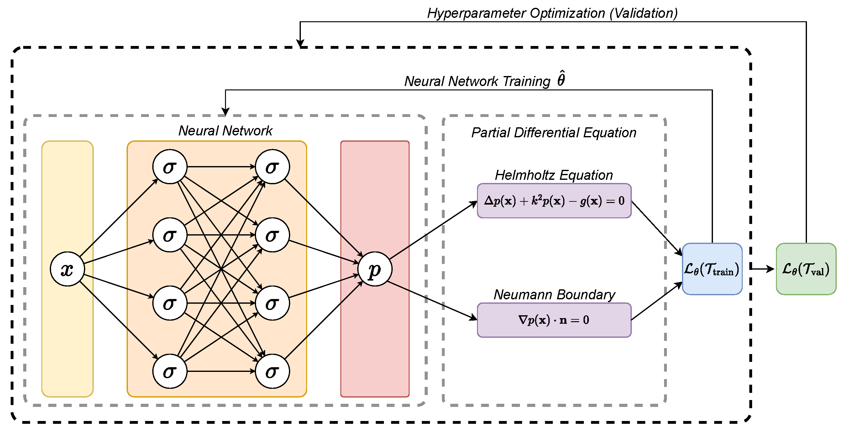
Figure 2.
The real part of the acoustic pressure at with NBC.
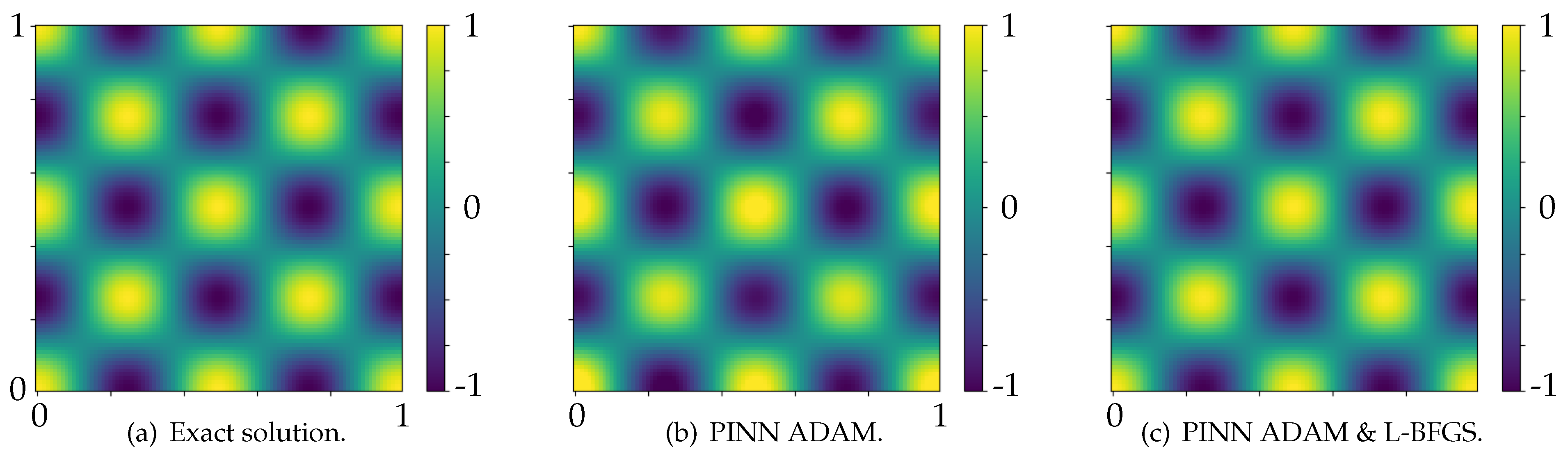
Figure 3.
Schematic representation of a LAAF-PINN. A neural network of L = 3 and N = 4 learns the mapping .
Figure 3.
Schematic representation of a LAAF-PINN. A neural network of L = 3 and N = 4 learns the mapping .
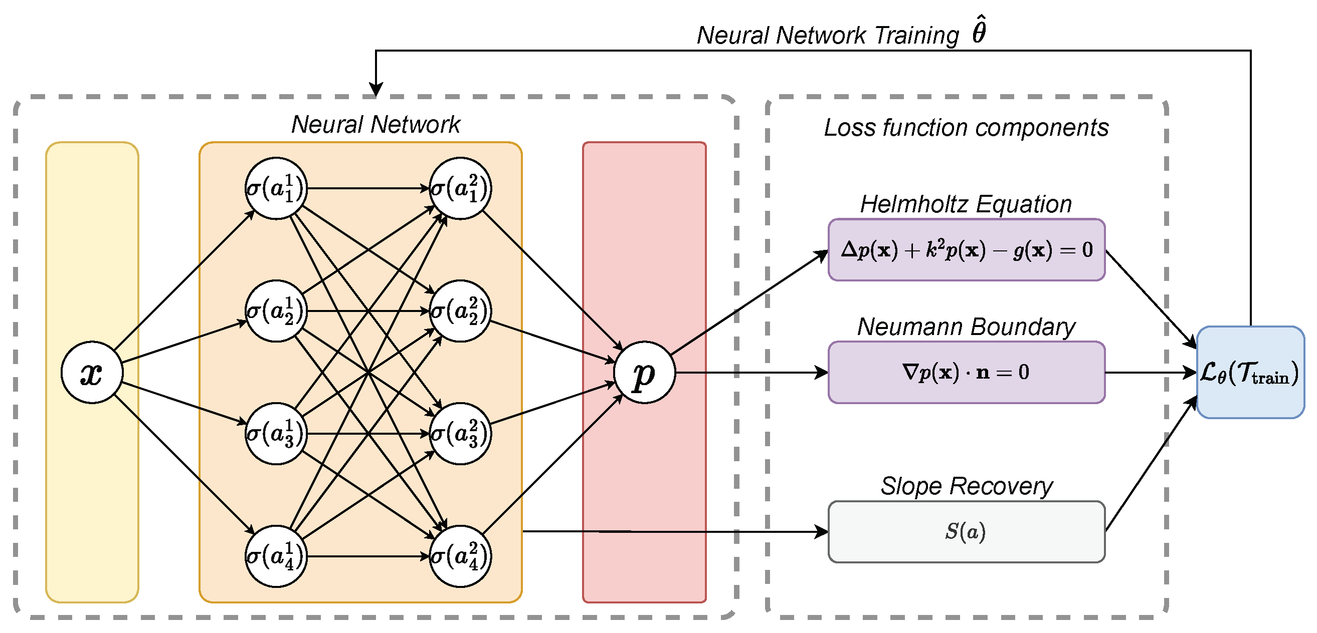
Figure 5.
Higher order oscillation and spatial dependence of the source and pressure based on the source sharpness parameter s.
Figure 5.
Higher order oscillation and spatial dependence of the source and pressure based on the source sharpness parameter s.
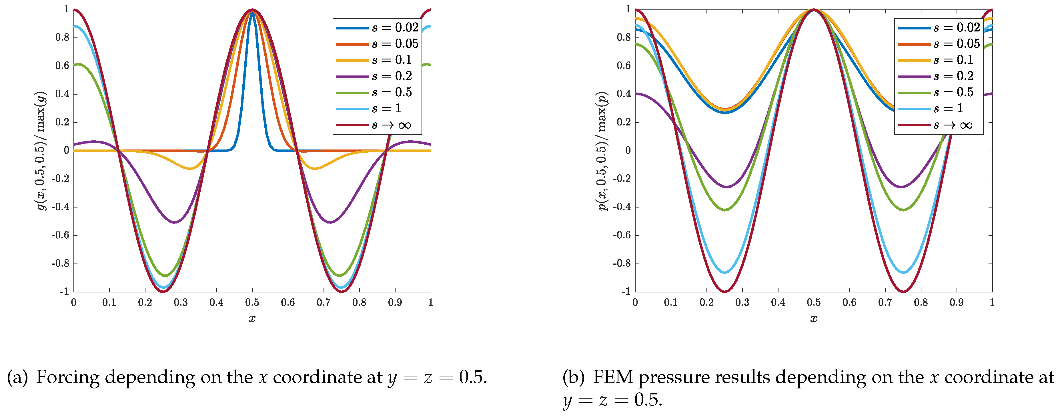
Figure 6.
Adaptive refinement for .
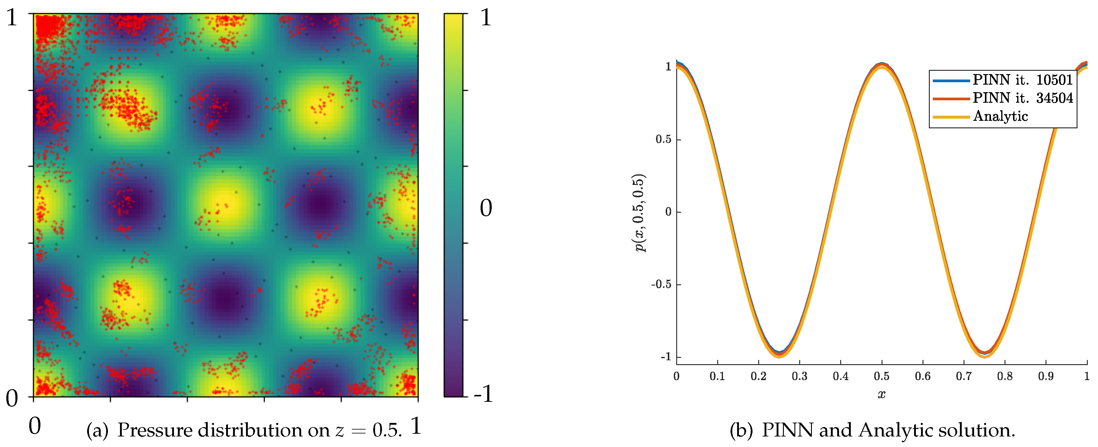
Figure 7.
Adaptive refinement for .
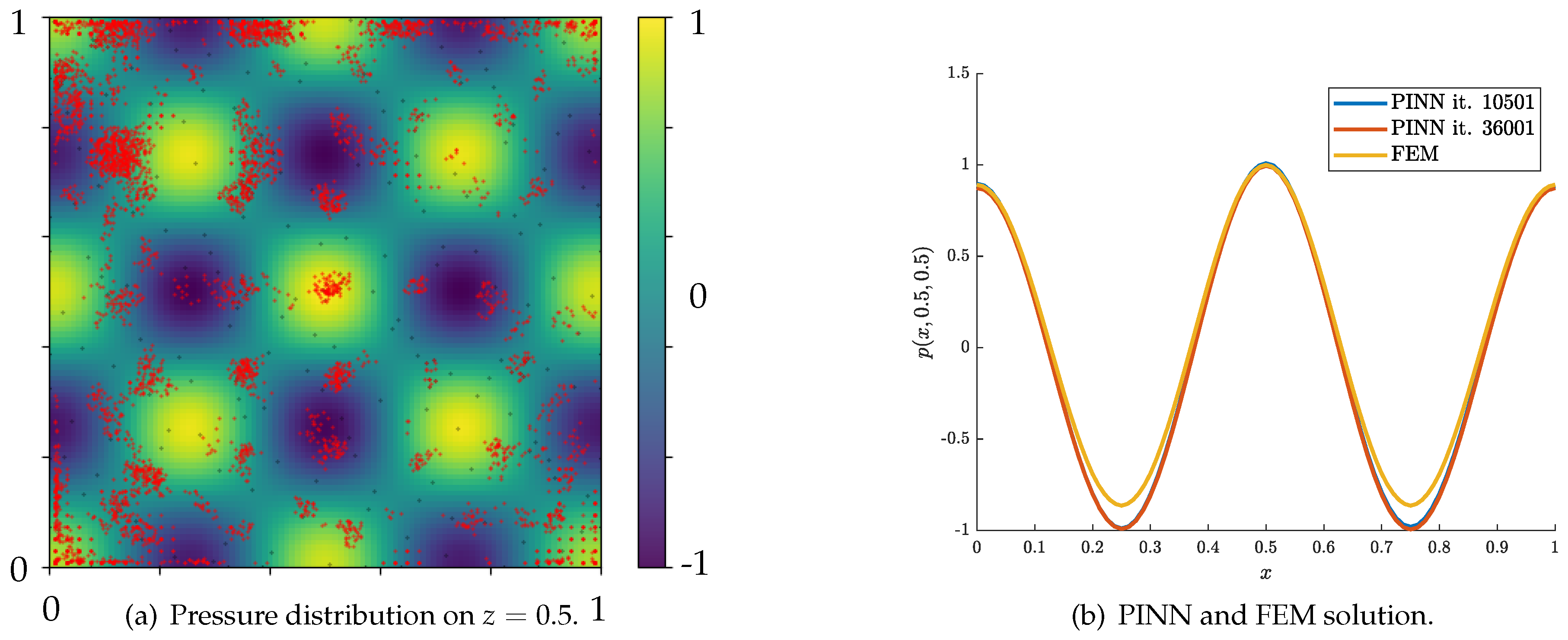
Figure 8.
Adaptive refinement for .
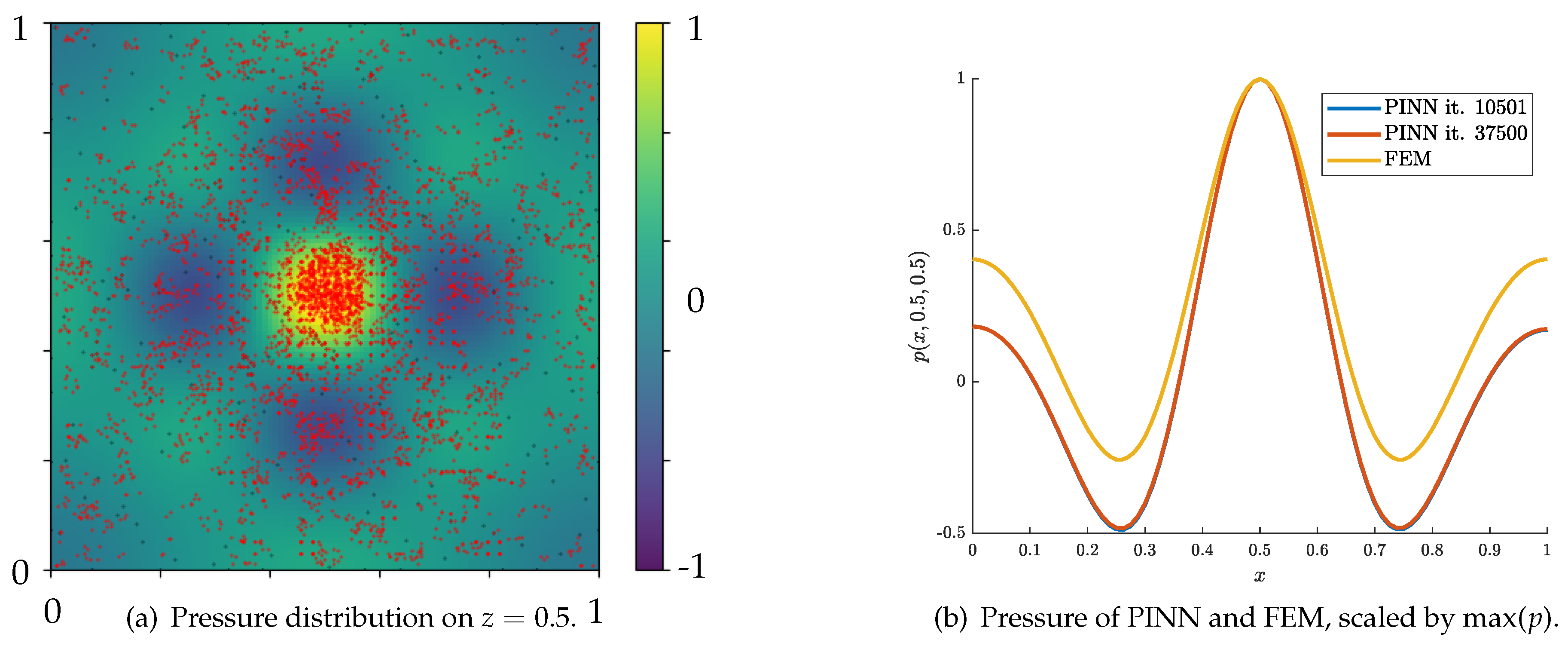
Figure 9.
Input feature generation depending on the wavelength and the results for various source sharpness parameter s.
Figure 9.
Input feature generation depending on the wavelength and the results for various source sharpness parameter s.
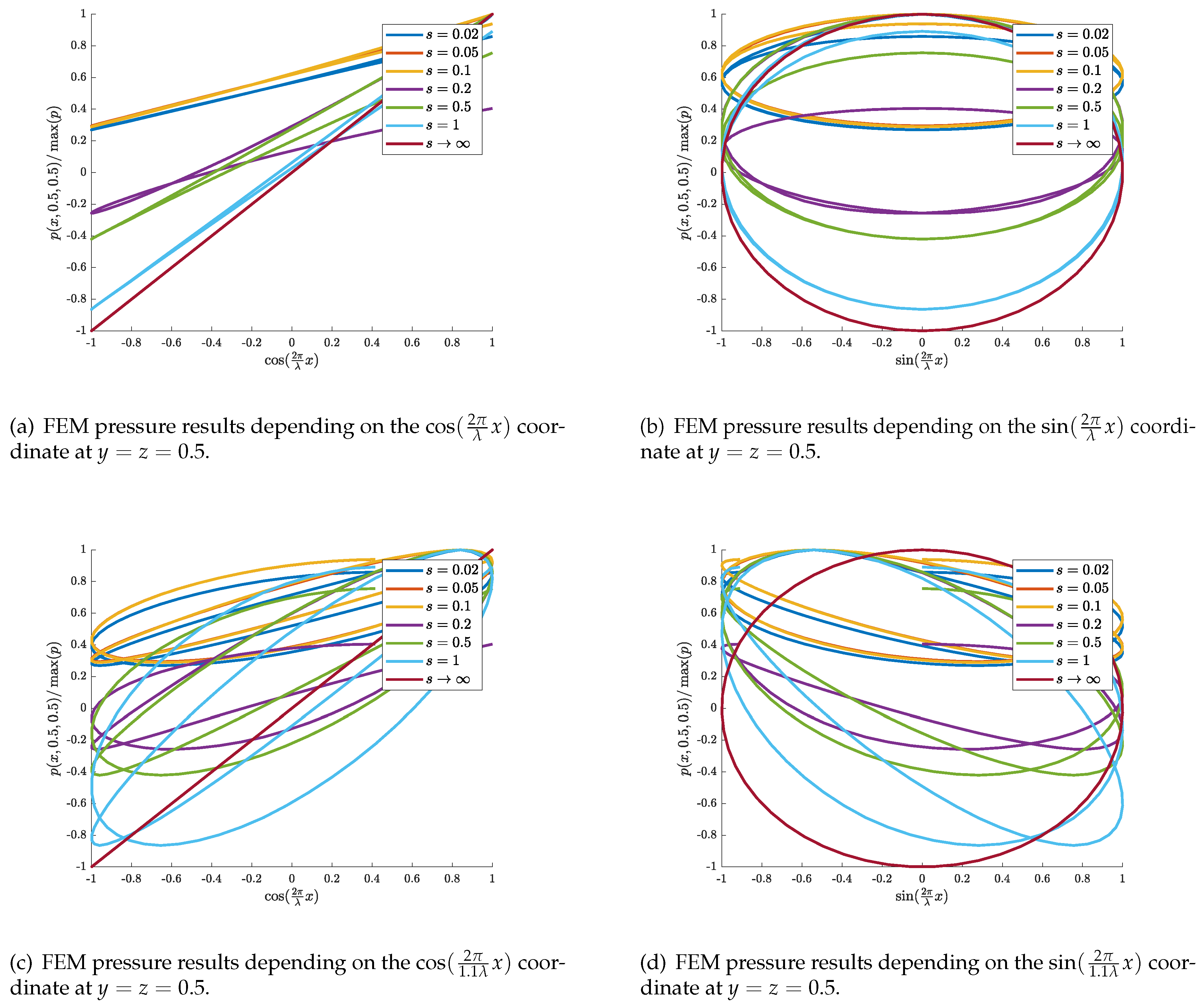
Figure 10.
Pressure results normalized by the maximum pressure of the reference (FEM, analytic) depending on the x coordinate at .
Figure 10.
Pressure results normalized by the maximum pressure of the reference (FEM, analytic) depending on the x coordinate at .
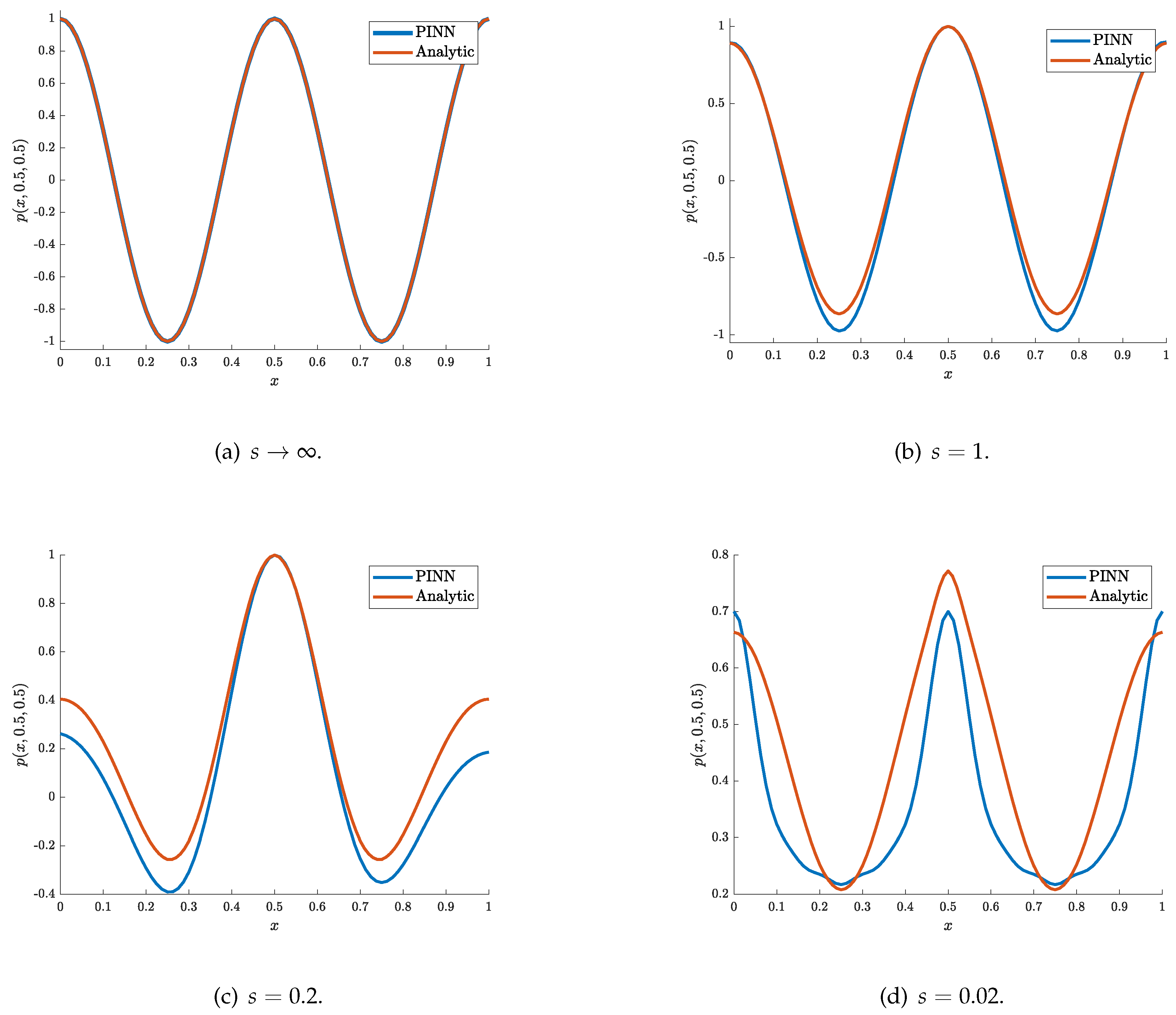

Table 1.
Deviations in percentage for various s parameters compared to a case of .
| s | in Pa | in % |
| 1 | 1.10 | 3.14 |
| 1.67 | 75.33 | |
| 1.56 | 112.87 | |
| 10.76 | - | |
| 6.12 | - | |
| 0.77 | 154.78 |
Table 2.
Error in percentage for number of layers and PDE/BC balancing weight hyperparameter of compared to FEM results. Yellow marked entries describe the best-performing parameter set in the direction of variation of the line search, and orange indicates the overall best value. For hyperparameters described as 5 + 50, 5 was chosen for the first step of the training sequence, with 90 000 Adams in this example, and then switched to 50 when continuing with the training by 15 000 iterations using LBFGS.
| W | training sequence | in % | ||||
| 1 | 180 | 5 | sin | P | 90 000 Adams | nc |
| 2 | 180 | 5 | sin | P | 90 000 Adams | 7.41 |
| 3 | 180 | 5 | sin | P | 90 000 Adams | 2.38 |
| 4 | 180 | 5 | sin | P | 90 000 Adams | 45.79 |
| 5 | 180 | 5 | sin | P | 90 000 Adams | 4.23 |
| 1 | 180 | 5 | sin | P | 90 000 Adams + 15 000 LBFGS | nc |
| 2 | 180 | 5 | sin | P | 90 000 Adams + 15 000 LBFGS | 7.4 |
| 3 | 180 | 5 | sin | P | 90 000 Adams + 15 000 LBFGS | 2.12 |
| 4 | 180 | 5 | sin | P | 90 000 Adams + 15 000 LBFGS | nc |
| 5 | 180 | 5 | sin | P | 90 000 Adams + 15 000 LBFGS | 3.17 |
| 1 | 180 | 5 + 50 | sin | P | 90 000 Adams + 15 000 LBFGS | nc |
| 2 | 180 | 5 + 50 | sin | P | 90 000 Adams + 15 000 LBFGS | 2.78 |
| 3 | 180 | 5 + 50 | sin | P | 90 000 Adams + 15 000 LBFGS | 1.91 |
| 4 | 180 | 5 + 50 | sin | P | 90 000 Adams + 15 000 LBFGS | nc |
| 5 | 180 | 5 + 50 | sin | P | 90 000 Adams + 15 000 LBFGS | 6.44 |
| 2 | 180 | 0.02 | sin | P | 90 000 Adams | 39.11 |
| 2 | 180 | 0.2 | sin | P | 90 000 Adams | 23.40 |
| 2 | 180 | 1 | sin | P | 90 000 Adams | 9.03 |
| 2 | 180 | 5 | sin | P | 90 000 Adams | 7.41 |
| 2 | 180 | 50 | sin | P | 90 000 Adams | 3.04 |
| 2 | 180 | 500 | sin | P | 90 000 Adams | 7.46 |
| 3 | 180 | 5 | sin | P | 90 000 Adams | 2.38 |
| 3 | 180 | 50 | sin | P | 90 000 Adams | 2.37 |
| 3 | 180 | 500 | sin | P | 90 000 Adams | 2.82 |
Table 3.
Error in percentage for layer width and backend as a hyperparameter-variation compared to FEM results. Yellow marked entries describe the best-performing parameter set in the direction of variation of the line search, and orange indicates the overall best value.
Table 3.
Error in percentage for layer width and backend as a hyperparameter-variation compared to FEM results. Yellow marked entries describe the best-performing parameter set in the direction of variation of the line search, and orange indicates the overall best value.
| W | training sequence | in % | ||||
| 2 | 20 | 5 | sin | P | 90 000 Adams | nc |
| 2 | 40 | 5 | sin | P | 90 000 Adams | 61.47 |
| 2 | 60 | 5 | sin | P | 90 000 Adams | nc |
| 2 | 120 | 5 | sin | P | 90 000 Adams | 3.50 |
| 2 | 180 | 5 | sin | P | 90 000 Adams | 7.41 |
| 2 | 240 | 5 | sin | P | 90 000 Adams | 6.86 |
| 2 | 300 | 5 | sin | P | 90 000 Adams | 6.68 |
| 3 | 20 | 5 | sin | P | 90 000 Adams | nc |
| 3 | 40 | 5 | sin | P | 90 000 Adams | nc |
| 3 | 60 | 5 | sin | P | 90 000 Adams | 2.72 |
| 3 | 120 | 5 | sin | P | 90 000 Adams | 2.21 |
| 3 | 180 | 5 | sin | P | 90 000 Adams | 2.38 |
| 3 | 240 | 5 | sin | P | 90 000 Adams | 2.53 |
| 3 | 300 | 5 | sin | P | 90 000 Adams | 3.61 |
| 2 | 20 | 50 | sin | P | 90 000 Adams | nc |
| 2 | 40 | 50 | sin | P | 90 000 Adams | nc |
| 2 | 60 | 50 | sin | P | 90 000 Adams | 3.73 |
| 2 | 120 | 50 | sin | P | 90 000 Adams | 3.39 |
| 2 | 180 | 50 | sin | P | 90 000 Adams | 4.69 |
| 3 | 20 | 50 | sin | P | 90 000 Adams | nc |
| 3 | 40 | 50 | sin | P | 90 000 Adams | 2.77 |
| 3 | 60 | 50 | sin | P | 90 000 Adams | nc |
| 3 | 120 | 50 | sin | P | 90 000 Adams | 3.47 |
| 3 | 180 | 50 | sin | P | 90 000 Adams | 2.37 |
| 2 | 120 | 50 | sin | P | 90 000 Adams | 3.39 |
| 3 | 120 | 50 | sin | P | 90 000 Adams | 3.47 |
| 2 | 120 | 50 | sin | TF1 | 90 000 Adams | 2.92 |
| 3 | 120 | 50 | sin | TF1 | 90 000 Adams | 1.99 |
| 2 | 120 | 50 | sin | TF2 | 90 000 Adams | 3.36 |
| 3 | 120 | 50 | sin | TF2 | 90 000 Adams | 3.28 |
Table 4.
Error in percentage for activation function as a hyperparameter-variation compared to FEM results. Yellow marked entries describe the best-performing parameter set in the direction of variation of the line search, and orange indicates the overall best value.
Table 4.
Error in percentage for activation function as a hyperparameter-variation compared to FEM results. Yellow marked entries describe the best-performing parameter set in the direction of variation of the line search, and orange indicates the overall best value.
| W | training sequence | in % | ||||
| 2 | 180 | 5 | sin | P | 90 000 Adams | 7.41 |
| 2 | 180 | 5 | ELU | P | 90 000 Adams | nc |
| 2 | 180 | 5 | GELU | P | 90 000 Adams | nc |
| 2 | 180 | 5 | ReLU | P | 90 000 Adams | nc |
| 2 | 180 | 5 | SELU | P | 90 000 Adams | nc |
| 2 | 180 | 5 | sigmoid | P | 90 000 Adams | nc |
| 2 | 180 | 5 | SiLU | P | 90 000 Adams | nc |
| 2 | 180 | 5 | swish | P | 90 000 Adams | 18.05 |
| 2 | 180 | 5 | tanh | P | 90 000 Adams | 20.84 |
Table 5.
Error in percentage for locally adaptive activation function network compared to FEM results.
Table 5.
Error in percentage for locally adaptive activation function network compared to FEM results.
| W | training sequence | in % | ||||
| 2 | 180 | 5 | sin | P | 90 000 Adams | 7.41 |
| 2 | 180 | 5 | LAAF-n 1 | TF1 | 90 000 Adams | 17.25 |
| 2 | 180 | 5 | LAAF-n 2 | TF1 | 90 000 Adams | 3.85 |
| 2 | 180 | 5 | LAAF-n 4 | TF1 | 90 000 Adams | nc |
| 2 | 180 | 5 | LAAF-n 8 | TF1 | 90 000 Adams | nc |
Disclaimer/Publisher’s Note: The statements, opinions and data contained in all publications are solely those of the individual author(s) and contributor(s) and not of MDPI and/or the editor(s). MDPI and/or the editor(s) disclaim responsibility for any injury to people or property resulting from any ideas, methods, instructions or products referred to in the content. |
© 2024 by the author. Licensee MDPI, Basel, Switzerland. This article is an open access article distributed under the terms and conditions of the Creative Commons Attribution (CC BY) license (https://creativecommons.org/licenses/by/4.0/).
Copyright: This open access article is published under a Creative Commons CC BY 4.0 license, which permit the free download, distribution, and reuse, provided that the author and preprint are cited in any reuse.


