Submitted:
22 November 2024
Posted:
24 November 2024
You are already at the latest version
Abstract
High-Definition (HD) maps aim to provide comprehensive road information with centimeter-level accuracy, essential for precise navigation and safe operation of Autonomous Vehicles (AVs). Traditional offline construction methods involve multiple complex steps—such as data collection, point cloud map generation, and feature extraction—which not only incur high costs but also struggle to adapt to the rapid changes in dynamic environments. In contrast, the online construction method utilizes onboard sensor data to dynamically generate local HD maps, providing a bird’s-eye view (BEV) representation of the surrounding road environment. This approach has the potential for superior scalability and adaptability, enabling more effective responses to the ever-evolving road conditions. In this survey, we examine the latest advancements in online HD map construction, aiming to bridge the gaps in existing literature. We analyze key advancements, methodologies, advantages, and disadvantages, along with future research directions.
Keywords:
High-Definition Map
; Online High-Definition Map Construction
; Autonomous vehicle
; Autonomous driving
1. Introduction
High-Definition (HD) maps, originating from navigation maps, are advanced digital maps that offer superior accuracy and a greater range of data dimensions. In contrast to conventional navigation maps, which typically achieve accuracy within the meter range, HD maps aim to provide absolute coordinate precision down to the centimeter level. Moreover, the scope of HD maps includes comprehensive static traffic-related information, with information such as (1) lane geometry data such as positions, widths, slopes, and curvatures, and (2) fixed infrastructure elements such as traffic signs, traffic lights and speed bumps [1]. The extensive information aims to improve the ability of Autonomous Vehicles (AVs) to perceive their surrounding environment, providing prior data for tasks such as localization, planning, control, and decision-making [2]. Based on geographic coverage and data granularity, HD maps can be classified as either global or local.
Specifically, the traditional global HD maps are built offline, which involve three main steps: data collection, point cloud map generation, and feature extraction [3]. First, data collection is performed using survey vehicles equipped with advanced sensors such as Light Detection and Ranging systems (LiDARs), cameras, radars, Global Navigation Satellite System (GNSS) receivers, and Inertial Measurement Units (IMUs). Then, the multimodal data is processed using algorithms such as Simultaneous Localization and Mapping (SLAM) [4,5], point cloud registration [6,7], and sensor fusion [8,9], to generate the initial point cloud map. Finally, relevant features encompassing road networks, lane markings, traffic signs, and traffic lights are extracted from the point cloud map using manual methods or machine learning techniques [10].
While the traditional offline HD map construction method can integrate data from multiple sources and support complex computation and analysis, it also faces some significant drawbacks. Firstly, the process is very costly. The data collection phase requires survey vehicles equipped with advanced sensors, which are expensive to purchase and maintain. Additionally, the feature extraction phase incurs further costs due to the need for personnel for manual labeling or high-performance computing equipment for running machine learning algorithms [3]. Secondly, it is challenging to maintain the accuracy and relevance of HD maps in dynamic environments. Environmental changes, such as road construction or alterations to traffic signs, can lead to discrepancies between the map and current conditions. As a result, static maps quickly become outdated, necessitating frequent and costly updates [2,11].
In this context, researchers have proposed algorithms [12,13,14,15] that leverage large-scale data and learning-based methods to construct HD maps online, attracting increasing attention. Concisely, we define the corresponding task as Online HD Map Construction that takes raw data from vehicle-mounted sensors as input and generates local HD maps as output. The raw data consists of multimodal sensor outputs, including camera images, LiDAR and radar point clouds, and IMU and GNSS data. The resulting HD map is a bird’s-eye view (BEV) representation of the surrounding road environment, primarily in rasterized or vectorized formats. This map includes information about static traffic elements, such as lane dividers, road boundaries, pedestrian crossings, traffic lights, and traffic signs.
The online method has the potential to offer advantages over the traditional offline method. First, the online method reduces mapping costs and demonstrates enhanced scalability [16]. It utilizes vehicle-mounted sensors for data collection and the onboard computing platform for real-time algorithm execution, eliminating the need for expensive survey fleets and manual annotation. Second, the online method adapts quickly to environmental changes and showcases superior adaptability [15]. It dynamically captures the surrounding traffic environment to construct and update local HD maps, ensuring the maps remain current. Third, the online method employs data-driven algorithms to improve generalization capabilities. It can potentially learn from large-scale datasets and apply this knowledge to new scenarios, which is particularly important for edge cases such as rural areas and nature reserves.
1.1. Comparison to Related Surveys
Although online HD map construction is an emerging and promising research area, comprehensive reviews on this topic are still limited. Recent reviews on BEV perception [17,18] have examined key perception tasks for AVs, such as 3D object detection, map segmentation, and sensor fusion, but have not sufficiently addressed the task of online HD map construction. Further, recent HD map reviews [1,2,3] have focused on map structure, functionality, offline construction and maintenance methods, whereas, the techniques of online HD map construction are overlooked in these surveys. Moreover, while Tang et al. [16] have examined both offline and online methods for HD map construction, their emphasis on traditional offline techniques might potentially limit the applicability of their findings, given the rapid advancements in this dynamic field. To fill these gaps, we aim to comprehensively review the latest progress in online HD map construction and provide a thorough analysis of key developments, existing challenges, and future research directions.
1.2. Contributions
The main contributions of this survey are:
- We provide background knowledge on online HD map construction, including key aspects such as task definitions, commonly used datasets, and prevalent evaluation metrics.
- We review the latest methods for online HD mapping, categorizing them based on the formats of local HD maps they produce. This review includes a comparative analysis and a detailed discussion of the strengths and limitations of methods within each category.
- We explore the current challenges, open problems, and future trends in this cutting-edge and promising research field. We offer insights to help readers understand the existing obstacles and identify areas needing further development.
1.3. Overview
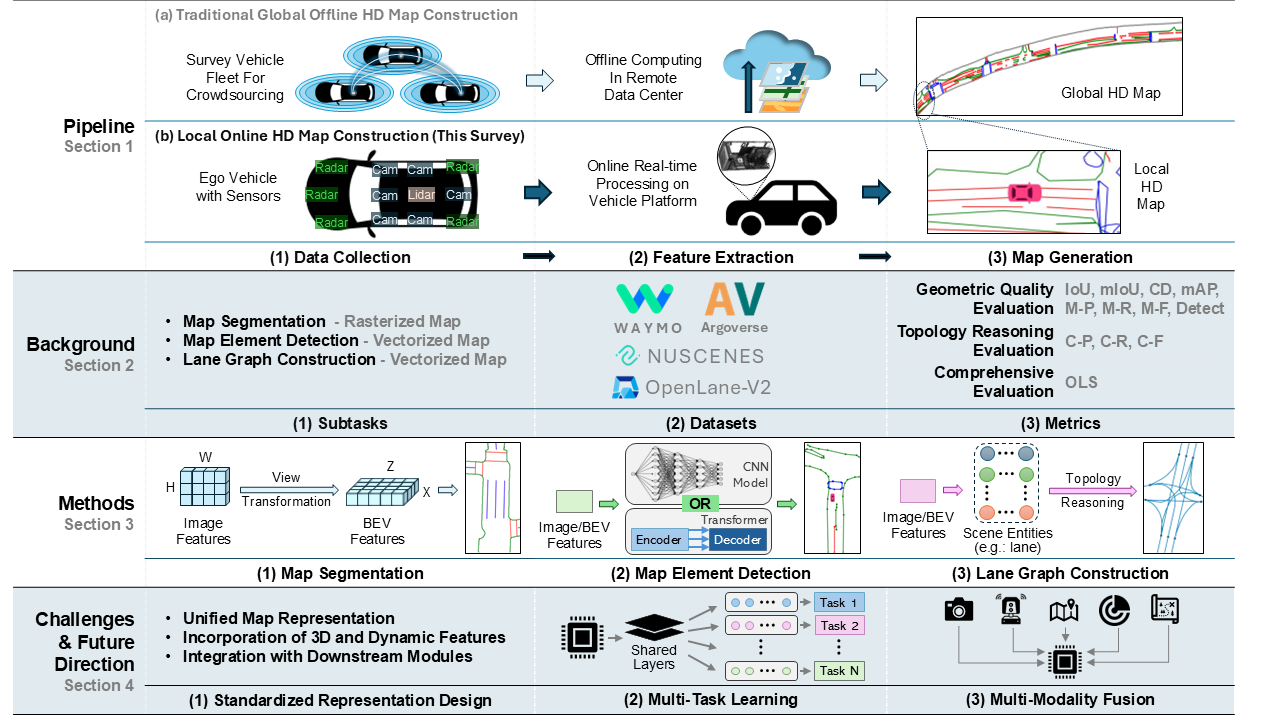
Figure 1 offers an overview of our survey. Section 1 introduces online HD map construction, highlighting its significance and research motivations. Section 2 presents background information, including task definitions, commonly used datasets, and evaluation metrics. Section 3 discusses the latest advancements categorized by output map format—map segmentation, map element detection, and lane graph construction—analyzing various methods and their strengths and weaknesses. Section 4 addresses current challenges and identifies potential future research directions. Section 5 concludes this paper.
2. Background
This section provides background knowledge on online HD map construction. For a comprehensive overview, we cover task definitions, commonly used datasets and prevalent evaluation metrics.
2.1. Task Definitions
We defined three sub-tasks in online HD map construction: Map Segmentation methods produce rasterized maps. In contrast, Map Element Detection and Lane Graph Construction methods generate vectorized maps.
Map Segmentation: This task leverages sensor observation data as input to dynamically create a rasterized map , which depicts the surrounding road environment of the ego vehicle as a grid of map pixels. Each pixel corresponds to a square area in the BEV and is assigned a map semantic category C that identifies the type of traffic control element present at that location. Here, H and W denote the height and width of the grid, respectively, while i and j represent spatial indices for each map pixel. This representation offers the ego vehicle the most fine-grained semantic and geometric information, allowing it to navigate and comply with traffic regulations.
Map Element Detection: This task leverages sensor observation data to dynamically create a vectorized map , detecting map elements within the ego vehicle’s surrounding road environment. Each element is represented by an ordered point sequence S to capture its geometric attributes and assigned a map semantic category C. Here, denotes the total number of vectorized map elements within . This representation provides the ego vehicle with instance-level semantic and geometric information for each map element, serving as an efficient sparse representation of the surrounding road environment.
Lane Graph Construction: This task leverages sensor observation data to dynamically create a vectorized map , depicting the ego vehicle’s surrounding road environment as a directed lane graph. This lane graph comprises a set of vertices and directed edges , with each edge connecting two vertices and indicating a direction from one vertex to another. Here, and denote the number of vertices and edges, respectively. The representation of the lane graph varies based on specific requirements, particularly regarding vertex and edge definitions. We will now introduce three common representations:
- Representation 1: Each vertex represents a point on the lane graph, defined by a vectorized sequence that encodes its coordinates and attributes. Each edge is a directed line segment connecting two vertices and is characterized by an ordered point sequence describing its geometric shape.
- Representation 2: Each vertex represents a lane, capturing its geometric shape with an ordered point sequence S. The edges are represented by an adjacency matrix I, where indicates that lane connects to lane , with the termination of lane aligned to the beginning of lane . Here, i and j are the indices of the lane vertices.
- Representation 3: Each vertex represents a lane or a traffic element, capturing its geometric shape with an ordered point sequence S. The edges are represented by two adjacency matrices: the first, , denotes the connectivity between lanes, where indicates that lane connects to lane , with the termination of lane aligned to the beginning of lane . The second adjacency matrix, , describes the correspondence between lanes and traffic elements, where signifies that lane is related to traffic element . Here, i and j are the indices of the lanes, and k is the index of the traffic elements.
2.2. Datasets
Table 1 shows common datasets for online HD map construction, among which nuScenes [20], Argoverse 2 [22], and Openlane-V2 [23] being the three most influential.
NuScenes Dataset. NuScenes [20] is a comprehensive multimodal autonomous driving dataset launched in 2019. It features 1,000 driving scenes recorded in Singapore and Boston, each lasting 20 seconds. The dataset is divided into 700 scenes for training, 150 for validation, and 150 for testing. NuScenes is notable for being the first dataset to include a full suite of AV sensors: 6 cameras with a resolution of 1600 × 900, a 32-beam spinning LiDAR, and 5 radars with a detection range of up to 250 meters, offering 360-degree environmental perception for AVs. In addition, NuScenes provides high-precision, human-annotated semantic maps in both rasterized and vectorized formats. The original rasterized maps cover only roads and sidewalks with a resolution of 10px/m. In contrast, the vectorized maps offer more detailed information with 11 semantic classes, including road dividers, lane dividers, and pedestrian crossings. These maps are instrumental as strong priors for downstream tasks such as prediction and planning.
Argoverse 2 Dataset. Argoverse 2 [22] is a comprehensive dataset for autonomous driving perception and prediction research, released in 2023 as an upgrade to the Argoverse [21] dataset. It features 1,000 diverse driving scenarios from six U.S. cities, each consisting of a 15-second multimodal data sequence, divided into 700 scenarios for training, 150 for validation, and 150 for testing. The dataset has an advanced sensor suite that provides a full panoramic field of view, including seven cameras with 2048 x 1550 pixel resolution, two roof-mounted 32-beam spinning LiDARs, and two stereo cameras of the same resolution. It also provides detailed 3D local HD maps in vectorized and rasterized formats. The vectorized maps include lane-level details such as lane boundaries, markings, crosswalks, and drivable areas, while the rasterized maps offer dense ground surface height data. This 3D map representation enhances lane geometry details, aiding AVs in better perceiving surrounding static traffic infrastructure.
OpenLane-V2 Dataset. OpenLane-V2 [23] is the first dataset designed to advance HD map construction through topology reasoning of traffic scene structures, launched in 2023. Building upon the existing nuScenes and Argoverse 2 datasets, it includes 2,000 diverse annotated road scenes divided into two subsets of 1,000 scenes each, with 700 scenes for training, 150 for validation, and 150 for testing. The dataset offers detailed annotations featuring vectorized HD maps and traffic elements. HD maps provide comprehensive information on lane segments, including centerlines, boundaries, marking types, and lane connectivity. Traffic elements such as traffic lights, road markings, and road signs are annotated within 2D bounding boxes on front-view images, and their relationships to lanes are represented as adjacency matrices for each frame. These detailed annotations and their relationships improve AVs’ comprehension of complex road environments, supporting more accurate navigation and decision-making.
2.3. Evaluation Metrics
Evaluating online HD map construction requires a comprehensive assessment framework due to its complex nature. Here, we group existing metrics into three categories: (1) Geometric Quality Evaluation that measures the precision of spatial and geometric attributes, (2) Topology Reasoning Evaluation that examines the connectivity and correspondence between map elements, and (3) Comprehensive Evaluation that provides an overall performance assessment by integrating multiple metrics.
2.3.1. Geometric Quality Evaluation
Intersection over Union (IoU). The most common metric to evaluate pixel-level localization performance in detection and segmentation tasks is the Intersection over Union () [16,24]. It assesses the similarity between the predicted representation () and the ground-truth geometry () by calculating the ratio of the intersection of the two areas () to their combined areas (). Accordingly, is mathematically defined as:
in which H and W refer to the height and width of the constructed map, respectively, and D corresponds to the category amount involved in the map. The value of ranges from 0 to 1, where higher values signify better alignment.
Mean Intersection over Union (mIoU). Various improvements have been proposed to enhance the clarity of . For instance, by taking the different semantic category of each detected or segmented map element into account, is computed by averaging the values across all classes. The corresponding mathematical definition is:
where D is the number of classes considered in the map.
Chamfer Distance (CD). is a Lagrangian metric that quantifies the spatial similarity between two vector geometric shapes, the predicted curve and the ground-truth one . It computes the average minimum squared distances between the constituent points on and , in both forward and backward directions [25]. Specifically, refers to the directional calculation from prediction to ground-truth, while denotes the directional calculation from ground-truth to prediction [25]. Hence, is mathematically defined as:
in which P and G represent the sets of points sampled on and the , respectively.
Mean Average Precision (mAP). serves as a classical metric to evaluate the accuracy of HD maps construction [16]. It quantifies the true positives in predictions compared to the ground truths. Specially, while conceptually similar to in 2D object detection, in HD map construction adopts or Frechet distance rather than as its matching criterion. And only if the corresponding distance is smaller than the threshold t, the prediction will be conceived as a true positive [16]. This adaptation accounts for the vector-based, geometric nature of HD map elements compared to pixel-based 2D images. Further, the threshold usually takes a value from the set [16]. Then, is computed by averaging the computed across all adopted thresholds. Hence, the corresponding mathematic definition is written as:
Centerline Identification Metrics (M-P, M-R, M-F, Detect). Similar to 2D classification tasks, fundamental evaluation metrics, Precision, Recall, and F1-score, have also been adapted to assess the accuracy of centerline identification in lane graph extraction. Specifically, these adapted metrics, denoted as , , and , evaluate how closely predicted centerlines align with the ground truths within a predefined distance threshold [12,26]. Meanwhile, since these metrics do not penalize cases where a ground truth centerline lacks any matching prediction, Detection Ratio () is proposed. It measures the fraction of ground truth centerlines that have at least one matching estimated centerline [12,26]. Hence, a low score combined with high scores on the other three metrics indicates a significant number of false negatives despite a satisfying performance in identifying true positives.
2.3.2. Topology Reasoning Evaluation
Connectivity Metrics (C-P, C-R, C-F). Given the crucial role of relation in graph interpretation, connectivity metrics are proposed to assess the accuracy of edge construction in lane graph. These metrics, , , and , are also adapted from standard precision and recall, while focus on how well the connectivity pattern of the predicted graph complies with that of the ground-truth graph [12,26].
2.3.3. Comprehensive Evaluation
OpenLane-V2 Score (). OLS incorporates four metrics to comprehensively evaluate the performance across three main subtasks supported by OpenLane-V2 dataset [23]. Specifically, , as a modified metric, assesses 3D lane detection performance, where Frechet distance serves as the matching criterion with threshold set meters. Similarly, appraises traffic element detection performance while using with threshold 0.75 as the affinity measure, to better aligned with the small-scaled nature of traffic elements. Further, and evaluate topology reasoning performance among centerlines or between lane centerlines and traffic elements, respectively. Hence, OLS is mathematically defined as:
where f is a scale function that weights the topology reasoning task.
3. Methods
This section explores various perspectives on online HD map construction. We categorize the methods into three sub-tasks based on the output map format: Map Segmentation in Section 3.1, Map Element Detection in Section 3.2, and Lane Graph Construction in Section 3.3.
Table 2 summarizes the literature on online HD map construction by sensor and task types. A growing number of studies are being published in prestigious conferences and journals, indicating a significant trend in developing these methods. Each method offers unique contributions, reflecting the vibrant research community dedicated to online HD map construction.
3.1. Map Segmentation for Rasterized Maps
Map segmentation algorithms dynamically generate rasterized maps representing the road environment around the ego vehicle as a pixel grid with semantic information. In this semantic understanding process, the camera captures visual details such as color, texture, and shape [85,86]. A key challenge in converting images to rasterized maps is that the input and output exist in different spaces: the former in the image plane and the latter in the BEV plane. To address this, mainstream vision-based map segmentation algorithms propose various view transformation (VT) methods to convert images or features from the 2D image plane to the 3D world space, decoding rasterized maps in the BEV.
Recent research [28,29,34,35,38] has focused on enhancing this VT module, leading us to categorize map segmentation methods into three main types based on VT techniques. The first category, "Projection-based Methods," employs the projection model defined by the camera’s intrinsic and extrinsic parameters to implement VT. The second category, "Lift-based Methods," involves a VT module that elevates images or features to 3D space by recovering depth information. The third category, "Network-based Methods," achieves VT implicitly through neural networks.
3.1.1. Projection-Based VT for Map Segmentation
Projection-based methods utilize the camera projection model for VT to generate rasterized maps. These methods trace back to inverse perspective mapping (IPM) [87], which converts perspective images into BEV images to eliminate distortion. It assumes that inverse-mapped points lie on a horizontal reference plane and employs the camera’s intrinsic and extrinsic parameters for converting pixels to world coordinates. While effective for preprocessing image-like data [88,89,90,91], IPM can introduce distortions when handling 3D objects. To address this, Cam2BEV [30] employs deep learning to correct these distortions. The method applies IPM for VT on feature maps from various cameras, followed by deep learning refinement to enhance the accuracy of the rasterized maps.
Other methods enhance the quality of rasterized maps by constructing 3D voxel features that retain high-dimensional information during VT. They initialize a voxel grid in world space and populate it with 2D feature maps, guided by the projection relationships defined by the camera’s intrinsic and extrinsic parameters. For example, MBEV [39] assumes a uniform depth distribution, filling the depth-direction voxels along the camera rays with corresponding 2D features, which are then height-compressed and decoded into a rasterized map. Simple-BEV [43], as depicted in Figure 2a, improves voxel quality by using bilinear sampling on the feature map for more effective grid filling.
Inspired by transformer architecture, methods combining camera projection relationships and cross-attention for constructing 3D voxel features have recently gained traction. BEVFormer [35] introduces a spatial cross-attention mechanism to generate BEV features adaptively. It first projects predefined grid-like BEV queries onto the 2D camera view, then uses a deformable attention mechanism [92] for interaction with sampled features in the regions of interest, and finally aggregates multi-view features to decode them into a rasterized map. Similarly, Ego3RT [36] (Figure 2b) introduces a multi-view adaptive attention mechanism that dynamically extracts key features from multi-view feature maps to generate 3D voxel features. By constructing BEV queries in a polarized coordinate system, this approach better aligns with the geometric distribution of the ego vehicle’s surroundings.
3.1.2. Lift-Based VT for Map Segmentation
Lift-based methods generate rasterized maps by recovering depth information from images for VT. Initially proposed by PON [28] (Figure 3a), this approach employs dense transformation layers made of multi-layer perceptrons (MLP). It begins with compressing feature maps along the height axis, then unfolds bottleneck features along the depth axis to create BEV features in polar coordinates. These features are resampled into an orthogonal coordinate system using camera parameters and then decoded into rasterized maps. Similarly, STA-ST [33] adopts this VT methodology and enhances it with temporal information and multi-scale supervision to improve map quality.
Other methods utilize convolutional neural networks (CNNs) to recover depth information from images at a granular level, enhancing the quality of rasterized maps. LSS [29], as shown in Figure 3b, was the first to use CNNs to predict depth probability distributions and contextual features for each pixel in the feature map. These are combined using an outer product to create frustum features with depth information. Finally, these frustum features are projected onto a unified BEV grid for fusion and decoded into a rasterized map. Subsequent methods adopted a similar VT approach, enhanced through deep supervision, spatiotemporal fusion, sensor fusion, and multitask learning. BEVerse [40] aligns past BEV features with current ones, feeding them into decoders for three distinct tasks to improve joint learning and optimization efficiency. In contrast, BEVFusion [42] integrates data from multi-view cameras and LiDAR, enabling the fused BEV features to support both 3D object detection and BEV map segmentation tasks effectively.
3.1.3. Network-Based VT for Map Segmentation
Network-based methods achieve VT by implicitly encoding camera projection relationships with neural networks. They originate from VPN [31], which uses an MLP to learn spatial dependencies between pixel and BEV coordinate systems. The process involves mapping feature maps to BEV space with a two-layer MLP and fusing multi-view feature maps to decode a rasterized map. However, the significant perspective differences between the perspective view and BEV can lead to information loss during direct feature mapping. To align features before and after mapping, PYVA [32] (Figure 4b) introduced cycled view projection. This method uses two MLPs for bidirectional transformations between the two spaces and employs cyclic consistency loss to ensure feature coherence during the conversion process.
Other methods utilize the transformer architecture to capture the camera projection relationship, significantly improving the quality of rasterized maps. Tesla [93] was the first to implement the cross-attention mechanism from this architecture to model the projection relationship. This approach constructs dense BEV queries and uses cross-attention to refine these queries through interaction with feature maps, ultimately decoding outputs for various perception tasks. However, the computational cost of traditional cross-attention increases quadratically with input size, leading to significant overhead when processing high-dimensional data. To address this, BEVSegFormer [41] (Figure 4b) utilizes deformable cross-attention [92], a sparse variant that generates 2D reference points for each BEV query using an MLP. It then dynamically samples the nearby regions of feature maps to refine the BEV queries for decoding the rasterized map.
Various methods integrate camera geometric information into image features during VT to enhance the model’s ability to capture geometric correspondences and improve cross-view fusion. CVT [34] pioneers camera-aware positional embeddings, converting pixel coordinates into 3D direction vectors that link geometric information across camera views. LaRa [37] follows a similar approach with ray embeddings. In contrast, PETRv2 [45] employs 3D position embeddings to enhance image features. The method maps points from the camera’s frustum space to 3D space. The 3D coordinates of these points are utilized to generate positional embeddings that integrate with image features, enhancing the model’s perception of three-dimensional object information.
3.1.4. Discussion on Map Segmentation Methods
Map segmentation methods can be classified into three types based on VT techniques, each with unique advantages and limitations. First, projection-based methods explicitly establish the coordinate transformation between pixels and BEV space using a camera projection model. While they offer strong interpretability through clear geometric frameworks, their performance heavily relies on the accuracy of camera parameters, which can be affected by factors like vibration and temperature changes during dynamic driving. Second, lift-based methods recover lost depth information from the camera to elevate images into 3D space. Although they provide an intuitive VT solution, they depend on the accuracy of depth estimation and often require additional sensors, such as stereo cameras or LiDAR, for improved depth precision. Lastly, network-based methods employ neural networks to learn camera projection relationships for VT implicitly. This straightforward approach reduces reliance on precise camera parameters but tends to converge more slowly and requires substantial data to achieve optimal performance. Therefore, an important research direction is effectively leveraging the complementary advantages of different VT techniques to enhance map segmentation performance.
Some methods combine various VT techniques to enhance the quality of rasterized maps. PanopticSeg [38] introduces an architecture with two VT modules for handling vertical and horizontal regions. The horizontal transformer uses IPM and an error correction module, while the vertical transformer lifts feature maps into a 3D voxel grid and resamples them using camera intrinsic parameters. This approach fuses the BEV features from both modules to produce the rasterized map. HFT [44] later adopts a similar dual-stream architecture, incorporating a mutual learning mechanism that enables the transformers to share information through feature imitation, improving overall accuracy.
Table 3 shows the results of map segmentation methods on the nuScenes [20] validation set, revealing two key observations. First, network-based methods significantly underperform other methods. For instance, in the single-camera setting, the mIoU of VED [94] and VPN [31] is only 25.2% and 31.8%, respectively. In the multi-camera setting, CVT [34] also performs poorly with a mIoU of just 40.2%. This may result from network-based methods not explicitly utilizing camera geometric information during the VT process. Second, incorporating LiDAR point clouds significantly enhances vision-based methods. For example, BEVFusion [42] saw a 6.1% increase in mIoU in a multi-camera setup after integrating LiDAR data. This improvement is likely due to the complementary information from cameras and LiDAR: cameras provide rich color and texture, while LiDAR offers precise distance measurements.
3.2. Map Element Detection for Vectorized Maps
Map element detection algorithms dynamically generate a vectorized map that includes traffic-related elements in the surrounding road environment, providing detailed geometric and semantic information. A key challenge in this process is detecting and classifying diverse map elements as ordered point sequences with semantic categories. This requires the algorithm to extract geometric shapes and classifications while managing occlusions from vehicles and pedestrians under varying lighting and weather conditions. To tackle this challenge, leading map element detection algorithms propose various Map Decoding (MD) techniques to transform image or BEV features into precise vectorized representations, reconstructing the surrounding environment’s structure and semantics.
Recent research [14,15,46,53] has focused on enhancing this MD module, enabling to classify map element detection methods into two main categories based on the decoder architecture. The first category, "CNN-based methods," employs CNN to process image or BEV features hierarchically, capturing local details and spatial structures for accurate map element detection. The second category, "Transformer-based methods," leverages the transformer’s self-attention mechanisms to capture long-range dependencies and global context in image or BEV features, enabling precise map element detection in complex road environments.
3.2.1. CNN-Based MD for Map Element Detection
CNN-based methods utilize CNN to process image or BEV features for detecting map elements. These methods were first introduced by HDMapNet [14] (Figure 5a), which uses a fully convolutional network [96] to detect map elements. Its decoder features three branches for semantic segmentation, instance embedding, and direction prediction. The outputs from the decoder are then post-processed through clustering and Non-Maximum Suppression (NMS), resulting in accurate and well-structured map elements. Building on this, SuperFusion [55] adopts a similar decoding approach and introduces a multi-level LiDAR-camera fusion mechanism to enhance long-range detection. The method includes data-level fusion using LiDAR depth to enhance images, feature-level fusion where image features guide LiDAR’s BEV features, and BEV-level fusion that aligns and merges BEV features from both modalities.
Some methods have introduced end-to-end CNN decoding strategies that streamline workflows and improve map element detection accuracy by reducing post-processing steps. InstaGraM [49], as depicted in Figure 5b, combines CNNs and a graph neural network (GNN) to extract and relate map elements. The method uses two CNNs to detect vertices and edges, then employs an attentional GNN to associate the vertices, ultimately generating vectorized representations that conform to road topology.
3.2.2. Transformer-Based MD for Map Element Detection
Transformer-based methods leverage Transformer’s self-attention mechanisms to capture long-range dependencies for precise map element detection. VectorMapNet [15] first employs a two-stage framework to decode the vectorized representation of map elements. The method first uses a DETR-like transformer [97] to extract key points from BEV features, followed by an autoregressive transformer that generates the vertex sequence for each map element. To address the efficiency bottleneck of autoregressive decoding in [15], MapTR [46] (Figure 6a) employs a single-stage decoder for parallel decoding. It initializes hierarchical queries with instance-level and point-level embeddings. It uses a DETR-like Transformer to enhance their interaction, producing an ordered point sequence for the detected elements. The follow-up work [66] introduces a one-to-many matching mechanism to speed up convergence and employs auxiliary dense supervision to enhance the performance of map element detection. MapVR [52] introduces rasterization to help the model capture intricate map details. It features a differentiable rasterizer that provides fine-grained geometric shape supervision for vectorized outputs. MapDistill [61] introduces a three-level cross-modal knowledge distillation framework that transfers knowledge from a camera-LiDAR fusion model to a camera model using a teacher-student approach.
Several methods improve the query and decoder designs in Transformer to enhance the accuracy of map element detection. HIMap [56] introduces HIQuery, a hybrid representation that integrates point-level and element-level information for map elements. Its hybrid decoder employs a point-element interaction module that iteratively fuses these information types, enabling accurate prediction of point coordinates and element shapes. In contrast, MapQR [65] proposes a "scattering and aggregation" mechanism to enhance instance queries. This mechanism distributes each query into sub-queries with distinct positional embeddings to gather features from different locations, which are then recombined into a unified instance query for enriched map element representations. MGMap [57], as shown in Figure 6b, leverages learned masks to enhance the detection of map elements. The method integrates global structural information from instance masks for accurate localization. It then extracts local semantic features from mask patches around predicted points to adjust point positions. Additionally, InsMapper [58] leverages point-wise correlations within map element instances to improve detection accuracy. The method enables information sharing and strengthens feature associations within each instance, resulting in smoother and more coherent map element detection in complex scenes. ADMap [64] reduces jitter in vectorized point sequences during map element detection.
Other methods improve the vectorized representation of map elements to enhance detection accuracy and efficiency. BeMapNet [47] employs piecewise Bezier curves to capture the shapes of complex map elements. The representation decomposes a curve into low-degree Bezier segments, each efficiently capturing local geometry with fewer control points to represent diverse map structures. PivotNet [50] introduces a pivot-based vectorized representation that selects key geometric points on map elements to create a compact and precise vectorized map. Additionally, ScalableMap [51] proposes a hierarchical sparse map representation that samples map elements at varying densities to balance computational cost and accuracy. DPFormer [54] introduces a compact Douglas-Peucker point representation. It selects key points based on curvature, increasing point density in curved sections while reducing points in straight sections, effectively minimizing redundancy and preserving map element structure. GeMap [59] proposes G-Representation. This approach uses displacement vectors between adjacent points to describe local geometric features of map instances, ensuring invariance to rotation and translation.
Several methods leverage short-term temporal information to improve map element detection’s accuracy and temporal consistency. StreamMapNet [53], as shown in Figure 7a, introduces a streaming temporal fusion mechanism that employs two strategies. Query propagation retains high-confidence element queries to the next frame, while BEV fusion aligns and fuses BEV features from consecutive frames. Building on this, SQD-MapNet [62] proposes a stream query denoising mechanism to improve the temporal consistency. The mechanism adds random noise to previous frame elements and then recovers the geometric shapes for the current frame through denoising, enhancing the model’s ability to capture temporal changes. In contrast, MapTracker [63] adopts a stacking strategy and introduces a dual-memory mechanism. The BEV memory module selects BEV features from historical frames by geometric distance and fuses them with current frame information. In contrast, the vector memory module filters historical map element queries by distance and refines current frame elements via per-instance cross-attention. PrevPredMap [69] integrates high-level information from previous predictions—such as map element categories, confidence, and location—into current frame predictions, improving the quality of map element detection.
Another direction is to leverage long-term temporal information derived from historical maps to enhance map element detection. NMP [48] introduces the concept of "neural map prior". The method employs cross-attention to integrate BEV features with global prior features, generating enhanced BEV features for improved detection. It then utilizes a gated recurrent unit (GRU) to dynamically update the global “neural map prior” with the enhanced BEV features. Similarly, HRMapNet [60] (Figure 7b) adopts a strategy that utilizes historical rasterized maps. The method designs a feature aggregation module to fuse BEV features with rasterized map features, enriching for improved map element detection. It then rasterizes the vectorized map predictions and maps them to the global map to facilitate continuous updates. Additionally, DTCLMapper [67] introduces a dual-temporal consistent module that leverages short- and long-term information. Using contrastive learning enhances temporal consistency by aligning same-category features across frames while distinguishing different ones. It also projects vectorized map predictions onto a global rasterized map, using occupancy constraints to ensure spatial consistency across frames. P-MapNet [68] introduces two map prior modules to improve distant map element detection. SDMap provides road skeleton information integrated with BEV features via cross-attention, while HDMap uses a masked autoencoder to learn HD map distribution patterns, refining predictions and correcting structures.
3.2.3. Discussion on Map Element Detection Methods
Map element detection methods can be classified into two types based on MD techniques, each with unique advantages and limitations. First, CNN-based methods utilize CNN to process the image or BEV features hierarchically, producing dense outputs transformed into vectorized representations of map elements via post-processing or association. While effectively extracting local features and reducing model complexity via weight sharing, they struggle with long-range dependencies, making them less suitable for map elements with long spatial spans like lanes and sidewalks. Second, Transformer-based methods utilize self-attention to capture relationships between patches in image or BEV features, enabling direct generation of vectorized representations through parallel or autoregressive decoding. This approach enhances understanding of long-range dependencies in geometric structures but also increases model complexity and computational demands, requiring significant training data for effective generalization in unseen road environments.
Table 4 shows the results of map element detection methods on the nuScenes [20] validation set, revealing two key observations. First, Transformer-based methods significantly outperform CNN-based methods. In the multi-camera setup, the worst Transformer-based method, InsMapper [58], has an mAP 11.6% higher than the best CNN-based method, InstaGraM [49]. In the multi-camera and LiDAR setup, InsMapper’s mAP exceeds that of HDMapNet [14] by 30.0%. This superiority is likely due to Transformers’ self-attention mechanism, which effectively captures long-range dependencies and global context, enhancing their ability to detect map elements that span large distances. Second, integrating LiDAR input modality significantly improves vision-based methods. For example, HDMapNet [14] achieves an 8.0% increase in mAP, ADMap [64] improves by 7.9%, and MGMap [57] rises by 6.9%. This enhancement results from supplementary information provided by LiDAR point clouds, including (1) 3D geometric information, such as vehicle points in lanes that offer context for map element detection, and (2) reflectance intensity, where the high reflectance of lane markings sharply contrasts with the low reflectance of rough road surfaces.
3.3. Lane Graph Construction for Vectorized Maps
Lane graph construction algorithms dynamically generate vectorized maps that depict the road environment around the ego vehicle as directed lane graphs, enriched with detailed geometric and topological information. A key challenge in this process is reasoning about the topological relationships between lanes and traffic elements within complex road environments. This encompasses the connectivity and adjacency of lanes (such as intersections, forks, and merges) and the correspondence between traffic elements and lanes. To tackle this challenge, leading lane graph construction algorithms propose various topology reasoning (TR) methods to effectively identify and analyze the intricate relationships within road scene structures, enhancing the accuracy and practicality of the generated lane graphs.
Recent research [12,26,74,75,82] has focused on enhancing this TR module, leading us to categorize lane graph construction methods into two main types based on TR techniques. The first category, "Single-step-based Methods", completes the TR of the entire lane graph in a single step using information from the driving scene. The second category, "Iteration-based Methods", conducts TR over iterative steps, where each step analyzes, reasons, and adjusts specific sections of the lane graph, resulting in a more refined topological structure.
3.3.1. Single-Step-Based TR for Lane Graph Construction
Single-step-based methods complete the TR of the lane graph in a single step, deducing the relationships between all lanes and traffic elements in the driving scene. These methods trace back to STSU [12], which infers lane connectivity in a lane graph in a single step using an association head. It first employs a DETR-like transformer [97] to process feature maps and extract lane queries. Then, MLP-based task heads decode the geometric and topological information from these queries, outputting lane existence probabilities, Bézier curve control points, and connection probabilities between lane pairs to construct a directed lane graph. LaneSegNet [76] adopts a similar TR approach to generate lane graphs from lane segment representations, simultaneously providing geometric, semantic, and topological information. In contrast, LaneGAP [80] adopts a post-processing strategy to convert individual lane predictions into a complete lane graph. This method discretizes lane predictions into vertices and merges nearby vertices to restore the topological structures of lane forks and merges.
High-quality detection is crucial for the TR of lane graphs, with some methods enhancing lane and traffic element detectors to achieve this. TopoMLP [77], as shown in Figure 8a, presents an efficient lane graph construction pipeline. It first uses a PETR-like transformer [102] to detect lanes and then integrates YOLOv8 as an auxiliary detector to enhance small traffic element detection. Finally, two MLP heads infer two types of topology relationships to generate a complete lane graph. Some methods [71,79] employ temporal aggregation with multi-frame information to address occlusion, enhancing the quality of generated lane graphs. LaneMapNet [79] introduces a curve region-aware attention mechanism, which learns curve-shape features to improve lane regression. Additionally, RoadPainter [84] introduces a point-mask optimization mechanism that generates instance masks from initial lane predictions, samples representative points, and fuses them with the original lane points to refine predictions.
Other methods enhance the topological accuracy of lane graphs by incorporating auxiliary supervision signals based on prior knowledge. TPLR [13] (Figure 8b) introduces minimal cycles in the lane graph—smallest closed curves formed by lane intersections—to accurately capture its topological structure. The method employs a transformer to process lane and cycle queries simultaneously, followed by an MLP to output the cover of minimal cycles, helping the model learn the correct order of lane intersections. Similarly, ObjectLane [73] models the relationship between traffic objects and lanes as a clustering problem, with lanes as cluster centers and traffic objects as data points. It uses a transformer to generate association information, assigning each detected object a probability distribution for its most likely corresponding lane. This approach ensures that the lane graph reflects road geometry and traffic participants’ distribution. LaneWAE [72] leverages the dataset’s prior distribution to enhance lane graph predictions. It uses a Transformer-based Wasserstein autoencoder to capture a latent space representation of lane structures. The method then refines initial predictions by optimizing latent space vectors to align with the learned prior.
3.3.2. Iteration-Based TR for Lane Graph Construction
Iteration-based methods conduct the TR of the lane graph in iterative steps, where each step analyzes, reasons, and adjusts specific relationships between lanes and traffic elements, gradually refining the overall structure. TopoNet [75], as depicted in Figure 9a, first leverages a scene GNN for the iterative refinement of lane graph topologies. It begins with a DETR-like transformer [97] to extract queries for lane and traffic elements, forming two initial graphs. A graph convolutional network (GCN) then performs iterative message passing and feature updating, refining the queries with spatial and semantic context from neighboring nodes, ultimately creating a comprehensive lane graph. Similarly, TopoLogic [82] employs an iterative TR pipeline that integrates two lane topologies to enhance reasoning in complex driving scenes. The method first calculates the geometric distances between predicted lanes to assess their connectivity, and then evaluates the similarity of lane queries in semantic space to address geometric reasoning limitations. Finally, it fuses the adjacency matrices from both topologies to create a more accurate lane graph. Additionally, CGNet [81] combines GCN with GRU to iteratively optimize the lane graph. The GRU’s memory mechanism retains information from previous layers, allowing TR to leverage both current data and accumulated knowledge. SMERF [78] combines road topology from SD maps with vehicle sensor data to enhance lane topology reasoning.
Recently, researchers have developed various mask-based mechanisms to improve lane detection. One significant approach is TopoMaskV2 [83], which employs a masked attention mechanism. The method generates Bezier control points and mask embeddings from lane queries, then focuses on the masked regions to update these queries effectively. It integrates the outputs from the mask head and Bezier head to achieve smoother and more accurate lane predictions.
Some methods perform local TR in a sequential manner to construct a complete lane graph. CenterLineDet [70] mimics expert annotators to construct a lane graph vertex by vertex. It utilizes the VT network to generate a BEV heatmap and extract the initial vertex set, while a DETR-like transformer [97] then iteratively predicts the next vertex position based on the ROI heatmap. Finally, the local lane graphs are combined to create a comprehensive global lane graph. In contrast, RoadNetTransformer [74] (Figure 9b) introduces the RoadNet Sequence representation, effectively capturing the topological structure of the lane graph for sequential TR. It features three transformer-based decoder architectures with distinct strategies: the semi-autoregressive version predicts lane key points in parallel and autoregressively generates the local sequences, while the non-autoregressive version performs full parallel predictions on the masked sequence and iteratively refines low-confidence tokens to enhance sequence quality. Similarly, LaneGraph2Seq [26] introduces a graph sequence representation for lane graphs. It employs an autoregressive Transformer to sequentially generate the vertex and edge sequences, ultimately reconstructing them into the complete lane graph structure.
3.3.3. Discussion on Lane Graph Construction Methods
Lane graph construction methods can be categorized into two types based on TR techniques, each with distinct advantages and limitations. First, single-step-based methods perform the TR of the entire lane graph in one step using driving scene information. They are easy to implement and short processing times, but one-step reasoning lacks flexibility, often leading to suboptimal performance in complex traffic scenarios. For example, in large intersections with intricate topological structures, a single-step approach may struggle to accurately capture the relationships among multiple lanes, turn lanes, and traffic signals. Second, iteration-based methods perform TR by reasoning and refining specific parts of the lane graph through multiple steps. While this approach allows for fine-tuning predictions and offers greater flexibility, it also incurs higher computational costs and longer processing times, making it challenging to respond effectively to sudden obstacles or changing traffic patterns. Therefore, a key research direction is to balance the accuracy and speed of TR to meet real-time demands while ensuring high-quality lane graphs.
Table 5 and Table 6 present the results of lane graph construction methods on the nuScenes [20] validation set and the OpenLane-V2 [23] dataset, revealing two key observations. First, iteration-based methods significantly outperform single-step-based methods. For example, LaneGraph2Seq [26] achieves the highest C-F score of 63.2 in Table 5, while TopoLogic [82] and TopoMaskV2 [83] secure the best OLS scores in Table 6—41.6 and 41.7 for subset A, and 39.6 and 43.9 for subset B, respectively. This superiority likely arises from their ability to iteratively analyze and refine lane graphs, enhancing TR in complex traffic scenes. Second, incorporating the SD map as an additional data source markedly improves the model’s TR ability. In Table 6, all three methods show significant OLS score increases after integrating the SD map—SMERF [78] (TopoNet) by 3.8, RoadPainter [84] by 3.7, and TopoLogic [82] by 3.5. This improvement stems from the SD map’s provision of crucial topological information, enhancing the model’s understanding of global road layouts and boosting accuracy in distant and occluded areas.
4. Challenges and Future Trends
4.1. Standardized Representation Design
A challenge in online HD map construction is the lack of a standardized representation. The three main representations, each with its strengths and limitations: (1) map pixel grids in map segmentation, which capture fine-grained details but cannot distinguish between instances like lanes and crosswalks and are costly in storage and computation; (2) vectorized lane lines in map element detection, which efficiently represent road geometry but lack topological information, such as lane relationships at intersections; and (3) centerlines and traffic elements in lane graph construction, which effectively capture road network topology but lack detailed lane features like type, direction, and width. Therefore, representation design is crucial for online HD map construction, affecting the description of the surrounding road environment and the transmission of structured information to the decision-making module.
An important research direction is to develop a unified map representation that combines the strengths of existing methods while addressing their limitations. LaneSegNet [76], as depicted in Figure 10, introduces lane segment representation, integrating vectorized lane lines, centerlines, and road attributes to capture geometric, semantic, and topological information. Specifically, it includes (1) geometric information, such as lane centerlines and boundaries, with offsets defining boundary positions and polygons delineating drivable areas; (2) semantic information, including lane types (e.g., traffic lanes, pedestrian crossings) and boundary line types (e.g., solid, dashed, invisible) to encode lane characteristics and traversability; (3) topological information, represented as a lane graph with nodes for lane segments and edges for connectivity, stored in an adjacency matrix to model lane relationships like merging and diverging.
Another research direction is enhancing map representations by adding 3D structures (e.g., interchanges, elevated roads) and dynamic features (e.g., traffic lights, road signs) to capture complex road environments better. For example, OpenLane-V2 [23] expands the centerline lane graph with 13 types of traffic elements, including traffic lights, directional signs, restrictive signs, and special maneuver signs, while defining their relationships with lanes. Future research could analyze the diverse and heterogeneous elements within traffic scenes and their intricate interactions to provide more detailed structured information for scene understanding.
The third research direction is designing map representations that integrate seamlessly with downstream modules. Gu et al. [103] (Figure 11) propose an uncertainty-based map representation that uses probabilistic modelling to output map elements’ positions, categories, and uncertainties. This approach significantly enhances its utility in trajectory prediction tasks. Specifically, positional uncertainty is modelled with a Laplace distribution to capture prediction errors, while categorical uncertainty reflects confidence levels via probability distributions. These uncertainties enable trajectory prediction models to dynamically adjust the weighting of map elements, improving accuracy, robustness, and training efficiency.
4.2. Multi-Task Learning
Multi-Task Learning (MTL) trains a single model to perform multiple related tasks simultaneously, providing distinct advantages over separate task-specific models. First, MTL reduces computational and storage demands by sharing model structures and parameters, reducing the need for multiple models and lowering inference costs. Second, MTL improves generalization by capturing complementary information across tasks, which helps prevent overfitting and enhances performance on new data [104]. Consequently, MTL is well-suited for online HD map construction, as it can effectively integrate complementary information from related tasks to create more comprehensive local HD maps.
Some methods integrate other perception and prediction tasks to enhance online HD map construction. These tasks include (1) semantic segmentation [63,64,65,66], which classifies different regions in an image to provide insights into their categories and boundaries, helping the model understand the scene’s semantic structure; (2) depth estimation [63,64,65,66], which infers the distance between image pixels and the camera, offering information on the spatial location and geometric shapes of objects for accurate 3D modeling; (3) 3D object detection [12,35,36,39,40,42,43,45,12], which identifies and locates traffic-related objects, providing details on their categories, sizes, and relative positions, thus contributing contextual information; and (4) motion prediction [40], which estimates future trajectories of objects, enhancing the model’s understanding of complex and dynamic traffic scenarios.
Another direction is integrating multiple map-related tasks to enhance online HD map construction. BeMapNet [47] (as depicted in Figure 12b) and PivotNet [50] introduce map segmentation and instance segmentation of map elements, addressing sparse supervision in map element detection. HIMap [56] adopts a similar MTL strategy, while MGMap [57] and MapTracker [63] each focus on one of the tasks. MapTRv2 [66] enhances map element detection by incorporating map segmentation, semantic segmentation and depth estimation from a perspective view. Later works [59,64,65] follow similar approaches. To combine map element detection with lane graph construction, LaneSegNet [76] introduces lane segment representation that captures both geometric boundaries and topological relationships. TopoMaskV2 [83] enhances lane detection with instance segmentation.
However, integrating perception and prediction tasks for multi-task learning in online HD map construction does not always improve performance and can even result in "negative transfer." For instance, as shown in Table 7, MBEV [39], BEVFormer [35], and PETRv2 [45] experience a decrease in map segmentation mIoU by 1.7%, 2.2%, and 2.3%, respectively, after integrating 3D object detection, while Ego3RT [36] sees a 9.3% increase. Similarly, BEVerse [40] shows a 4.5% drop in mIoU after integrating both 3D object detection and motion prediction. In contrast, Table 8 demonstrates that MapTRv2 [66] achieves increases of 5.1%, 6.4%, and 7.0% in map element prediction mAP by progressively integrating depth estimation, map segmentation, and semantic segmentation. Future research could explore the relationships between online HD map construction and other tasks to drive performance improvements.
4.3. Multi-Modality Fusion
Multi-Modality Fusion (MMF) combines data from different modalities—such as images, point clouds, and SD maps—for processing and analysis. Each AV sensor has unique strengths and limitations [105]: 1) cameras capture rich visual details like color and texture but are sensitive to lighting, weather, and lack depth; 2) LiDAR provides precise depth data and functions in day or night but lacks color/texture and can be affected by extreme weather; and 3) radar is robust to lighting and harsh weather, detects object velocity, but has lower resolution and cannot capture precise shapes. In addition, SD maps offer basic road structures with broad coverage and low cost but lack high-precision traffic details, such as lane markings, traffic signs, and signals. Consequently, MMF is well-suited for online HD map construction, as it can effectively integrate complementary information from multi-modal data to create more accurate local HD maps.
Some methods integrate data from multiple sensors to enhance online HD map construction. BEVFusion [42], as depicted in Figure 13a, pioneers the fusion of camera and LiDAR data in the BEV space. The method projects camera and LiDAR features into a unified BEV space, concatenates them, and uses a convolutional BEV encoder to resolve local misalignment. Subsequent studies [14,57,64,66,68] adopt a similar middle fusion strategy. Simple-BEV [43] enhances performance by fusing camera and radar data, achieving near-LiDAR accuracy without relying on LiDAR. Additionally, SuperFusion [55] introduces a multi-level fusion technique to combine LiDAR and camera inputs, enabling long-range map element detection at distances up to 90 meters.
Another direction is to integrate SD maps and other prior maps to enhance online HD map construction. SMERF [78] uses road topology from SD maps to improve lane graph construction. The method first encodes polyline sequences from SD maps, then extracts road topology using a Transformer encoder, and finally fuses SD map features with BEV features through multi-head cross-attention. Subsequent works [82,84] adopt a similar strategy for integrating SD map data. In contrast, P-MapNet [68] rasterizes SD maps, encodes them with CNNs, and adaptively fuses SD map features with BEV features. NMP [48], as shown in Figure 13b, constructs global neural map priors from BEV features of previous traversals, enhancing local map inference. Similarly, HRMapNet [60] uses historical rasterized maps to complement online perception data. DTCLMapper [67] maintains a grid map and uses occupancy states to ensure the geometric consistency of map elements.
As shown in Table 9, combining online HD map construction with global prior maps significantly boosts performance. For example, HDMapNet [14] improves by 3.0% mAP with SD maps, VectorMapNet [15] gains 3.9% with a neural map prior, and StreamMapNet [53] and MapTRv2 [66] see 5.9% and 5.7% increases with historical rasterized maps. These results highlight the importance of prior maps in enhancing local map inference. Future research could explore more efficient integration of various prior maps with online HD map construction to optimize performance in complex driving scenarios.
5. Conclusion
In this survey, we provide a comprehensive review of recent research on online HD map construction, highlighting its significance, key advancements, methodologies, and future directions. We categorize methods into three sub-tasks—map segmentation, map element detection, and lane graph construction—and analyze their strengths and weaknesses. We hope this survey will offer valuable insights for the research community and inspire further exploration on online HD map construction.
References
- Liu, R.; Wang, J.; Zhang, B. High definition map for automated driving: Overview and analysis. The Journal of Navigation 2020, 73, 324–341. [Google Scholar] [CrossRef]
- Elghazaly, G.; Frank, R.; Harvey, S.; Safko, S. High-definition maps: Comprehensive survey, challenges and future perspectives. IEEE Open Journal of Intelligent Transportation Systems 2023. [Google Scholar] [CrossRef]
- Bao, Z.; Hossain, S.; Lang, H.; Lin, X. A review of high-definition map creation methods for autonomous driving. Engineering Applications of Artificial Intelligence 2023, 122, 106125. [Google Scholar] [CrossRef]
- Zhang, J.; Singh, S. LOAM: Lidar odometry and mapping in real-time. Robotics: Science and systems. Berkeley, CA, 2014, Vol. 2, pp. 1–9.
- Shan, T.; Englot, B.; Meyers, D.; Wang, W.; Ratti, C.; Rus, D. Lio-sam: Tightly-coupled lidar inertial odometry via smoothing and mapping. 2020 IEEE/RSJ international conference on intelligent robots and systems (IROS). IEEE, 2020, pp. 5135–5142. [CrossRef]
- Yi, S.; Worrall, S.; Nebot, E. Geographical map registration and fusion of lidar-aerial orthoimagery in gis. 2019 IEEE Intelligent Transportation Systems Conference (ITSC). IEEE, 2019, pp. 128–134. [CrossRef]
- Huang, X.; Mei, G.; Zhang, J. Feature-metric registration: A fast semi-supervised approach for robust point cloud registration without correspondences. Proceedings of the IEEE/CVF conference on computer vision and pattern recognition, 2020, pp. 11366–11374. [CrossRef]
- Shan, M.; Narula, K.; Worrall, S.; Wong, Y.F.; Perez, J.S.B.; Gray, P.; Nebot, E. A Novel Probabilistic V2X Data Fusion Framework for Cooperative Perception. 2022 IEEE 25th International Conference on Intelligent Transportation Systems (ITSC). IEEE, 2022, pp. 2013–2020. [CrossRef]
- Berrio, J.S.; Shan, M.; Worrall, S.; Nebot, E. Camera-LIDAR integration: Probabilistic sensor fusion for semantic mapping. IEEE Transactions on Intelligent Transportation Systems 2021, 23, 7637–7652. [Google Scholar] [CrossRef]
- Berrio, J.S.; Zhou, W.; Ward, J.; Worrall, S.; Nebot, E. Octree map based on sparse point cloud and heuristic probability distribution for labeled images. 2018 IEEE/RSJ International Conference on Intelligent Robots and Systems (IROS). IEEE, 2018, pp. 3174–3181. [CrossRef]
- Berrio, J.S.; Worrall, S.; Shan, M.; Nebot, E. Long-term map maintenance pipeline for autonomous vehicles. IEEE Transactions on Intelligent Transportation Systems 2021, 23, 10427–10440. [Google Scholar] [CrossRef]
- Can, Y.B.; Liniger, A.; Paudel, D.P.; Van Gool, L. Structured bird’s-eye-view traffic scene understanding from onboard images. Proceedings of the IEEE/CVF International Conference on Computer Vision, 2021, pp. 15661–15670. [CrossRef]
- Can, Y.B.; Liniger, A.; Paudel, D.P.; Van Gool, L. Topology preserving local road network estimation from single onboard camera image. Proceedings of the IEEE/CVF Conference on Computer Vision and Pattern Recognition, 2022, pp. 17263–17272. [CrossRef]
- Li, Q.; Wang, Y.; Wang, Y.; Zhao, H. Hdmapnet: An online hd map construction and evaluation framework. 2022 International Conference on Robotics and Automation (ICRA). IEEE, 2022, pp. 4628–4634. [CrossRef]
- Liu, Y.; Yuan, T.; Wang, Y.; Wang, Y.; Zhao, H. Vectormapnet: End-to-end vectorized hd map learning. International Conference on Machine Learning. PMLR, 2023, pp. 22352–22369.
- Tang, X.; Jiang, K.; Yang, M.; Liu, Z.; Jia, P.; Wijaya, B.; Wen, T.; Cui, L.; Yang, D. High-Definition Maps Construction Based on Visual Sensor: A Comprehensive Survey. IEEE Transactions on Intelligent Vehicles 2023. [Google Scholar] [CrossRef]
- Ma, Y.; Wang, T.; Bai, X.; Yang, H.; Hou, Y.; Wang, Y.; Qiao, Y.; Yang, R.; Manocha, D.; Zhu, X. Vision-centric bev perception: A survey. arXiv 2022, arXiv:2208.02797 2022. [Google Scholar] [CrossRef] [PubMed]
- Li, H.; Sima, C.; Dai, J.; Wang, W.; Lu, L.; Wang, H.; Zeng, J.; Li, Z.; Yang, J.; Deng, H.; others. Delving into the devils of bird’s-eye-view perception: A review, evaluation and recipe. IEEE Transactions on Pattern Analysis and Machine Intelligence, 2023. [CrossRef]
- Sun, P.; Kretzschmar, H.; Dotiwalla, X.; Chouard, A.; Patnaik, V.; Tsui, P.; Guo, J.; Zhou, Y.; Chai, Y.; Caine, B.; others. Scalability in perception for autonomous driving: Waymo open dataset. Proceedings of the IEEE/CVF conference on computer vision and pattern recognition, 2020, pp. 2446–2454. [CrossRef]
- Caesar, H.; Bankiti, V.; Lang, A.H.; Vora, S.; Liong, V.E.; Xu, Q.; Krishnan, A.; Pan, Y.; Baldan, G.; Beijbom, O. nuscenes: A multimodal dataset for autonomous driving. Proceedings of the IEEE/CVF conference on computer vision and pattern recognition, 2020, pp. 11621–11631. [CrossRef]
- Chang, M.F.; Lambert, J.; Sangkloy, P.; Singh, J.; Bak, S.; Hartnett, A.; Wang, D.; Carr, P.; Lucey, S.; Ramanan, D.; others. Argoverse: 3d tracking and forecasting with rich maps. Proceedings of the IEEE/CVF conference on computer vision and pattern recognition, 2019, pp. 8748–8757. [CrossRef]
- Wilson, B.; Qi, W.; Agarwal, T.; Lambert, J.; Singh, J.; Khandelwal, S.; Pan, B.; Kumar, R.; Hartnett, A.; Pontes, J.K.; others. Argoverse 2: Next generation datasets for self-driving perception and forecasting. arXiv, 2023; arXiv:2301.00493 2023.
- Wang, H.; Li, T.; Li, Y.; Chen, L.; Sima, C.; Liu, Z.; Wang, B.; Jia, P.; Wang, Y.; Jiang, S.; others. Openlane-v2: A topology reasoning benchmark for unified 3d hd mapping. Advances in Neural Information Processing Systems 2024, 36.
- Blaschko, M.B.; Lampert, C.H. Learning to Localize Objects with Structured Output Regression. Computer Vision – ECCV 2008; Forsyth, D., Torr, P., Zisserman, A., Eds.; Springer Berlin Heidelberg: Berlin, Heidelberg, 2008; pp. 2–15. [Google Scholar]
- He, Y.; Bian, C.; Xia, J.; Shi, S.; Yan, Z.; Song, Q.; Xing, G. VI-Map: Infrastructure-Assisted Real-Time HD Mapping for Autonomous Driving. Proceedings of the 29th Annual International Conference on Mobile Computing and Networking; Association for Computing Machinery: New York, NY, USA, 2023; ACM MobiCom ’23. [CrossRef]
- Peng, R.; Cai, X.; Xu, H.; Lu, J.; Wen, F.; Zhang, W.; Zhang, L. LaneGraph2Seq: Lane Topology Extraction with Language Model via Vertex-Edge Encoding and Connectivity Enhancement. arXiv, 2024; arXiv:2401.17609 2024. [Google Scholar]
- Liao, Y.; Xie, J.; Geiger, A. Kitti-360: A novel dataset and benchmarks for urban scene understanding in 2d and 3d. IEEE Transactions on Pattern Analysis and Machine Intelligence 2022, 45, 3292–3310. [Google Scholar] [CrossRef] [PubMed]
- Roddick, T.; Cipolla, R. Predicting semantic map representations from images using pyramid occupancy networks. Proceedings of the IEEE/CVF Conference on Computer Vision and Pattern Recognition, 2020, pp. 11138–11147. [CrossRef]
- Philion, J.; Fidler, S. Lift, splat, shoot: Encoding images from arbitrary camera rigs by implicitly unprojecting to 3d. Computer Vision–ECCV 2020: 16th European Conference, Glasgow, UK, August 23–28, 2020, Proceedings, Part XIV 16. Springer, 2020, pp. 194–210. [CrossRef]
- Reiher, L.; Lampe, B.; Eckstein, L. A sim2real deep learning approach for the transformation of images from multiple vehicle-mounted cameras to a semantically segmented image in bird’s eye view. 2020 IEEE 23rd International Conference on Intelligent Transportation Systems (ITSC). IEEE, 2020, pp. 1–7. [CrossRef]
- Pan, B.; Sun, J.; Leung, H.Y.T.; Andonian, A.; Zhou, B. Cross-view semantic segmentation for sensing surroundings. IEEE Robotics and Automation Letters 2020, 5, 4867–4873. [Google Scholar] [CrossRef]
- Yang, W.; Li, Q.; Liu, W.; Yu, Y.; Ma, Y.; He, S.; Pan, J. Projecting your view attentively: Monocular road scene layout estimation via cross-view transformation. Proceedings of the IEEE/CVF conference on computer vision and pattern recognition, 2021, pp. 15536–15545. [CrossRef]
- Saha, A.; Mendez, O.; Russell, C.; Bowden, R. Enabling spatio-temporal aggregation in birds-eye-view vehicle estimation. 2021 ieee international conference on robotics and automation (icra). IEEE, 2021, pp. 5133–5139. [CrossRef]
- Zhou, B.; Krähenbühl, P. Cross-view transformers for real-time map-view semantic segmentation. Proceedings of the IEEE/CVF conference on computer vision and pattern recognition, 2022, pp. 13760–13769. [CrossRef]
- Li, Z.; Wang, W.; Li, H.; Xie, E.; Sima, C.; Lu, T.; Qiao, Y.; Dai, J. Bevformer: Learning bird’s-eye-view representation from multi-camera images via spatiotemporal transformers. European conference on computer vision. Springer, 2022, pp. 1–18. [CrossRef]
- Lu, J.; Zhou, Z.; Zhu, X.; Xu, H.; Zhang, L. Learning ego 3d representation as ray tracing. European Conference on Computer Vision. Springer, 2022, pp. 129–144. [CrossRef]
- Bartoccioni, F.; Zablocki, É.; Bursuc, A.; Pérez, P.; Cord, M.; Alahari, K. Lara: Latents and rays for multi-camera bird’s-eye-view semantic segmentation. Conference on Robot Learning. PMLR, 2023, pp. 1663–1672. [CrossRef]
- Gosala, N.; Valada, A. Bird’s-eye-view panoptic segmentation using monocular frontal view images. IEEE Robotics and Automation Letters 2022, 7, 1968–1975. [Google Scholar] [CrossRef]
- Xie, E.; Yu, Z.; Zhou, D.; Philion, J.; Anandkumar, A.; Fidler, S.; Luo, P.; Alvarez, J.M. BEV: Multi-Camera Joint 3D Detection and Segmentation with Unified Birds-Eye View Representation. arXiv, 2022; arXiv:2204.05088 2022. [Google Scholar]
- Zhang, Y.; Zhu, Z.; Zheng, W.; Huang, J.; Huang, G.; Zhou, J.; Lu, J. Beverse: Unified perception and prediction in birds-eye-view for vision-centric autonomous driving. arXiv, 2022; arXiv:2205.09743 2022. [Google Scholar]
- Peng, L.; Chen, Z.; Fu, Z.; Liang, P.; Cheng, E. BEVSegFormer: Bird’s Eye View Semantic Segmentation From Arbitrary Camera Rigs. Proceedings of the IEEE/CVF Winter Conference on Applications of Computer Vision, 2023, pp. 5935–5943. [CrossRef]
- Liu, Z.; Tang, H.; Amini, A.; Yang, X.; Mao, H.; Rus, D.L.; Han, S. Bevfusion: Multi-task multi-sensor fusion with unified bird’s-eye view representation. 2023 IEEE international conference on robotics and automation (ICRA). IEEE, 2023, pp. 2774–2781. [CrossRef]
- Harley, A.W.; Fang, Z.; Li, J.; Ambrus, R.; Fragkiadaki, K. Simple-bev: What really matters for multi-sensor bev perception? 2023 IEEE International Conference on Robotics and Automation (ICRA). IEEE, 2023, pp. 2759–2765. [CrossRef]
- Zou, J.; Zhu, Z.; Huang, J.; Yang, T.; Huang, G.; Wang, X. HFT: Lifting Perspective Representations via Hybrid Feature Transformation for BEV Perception. 2023 IEEE International Conference on Robotics and Automation (ICRA). IEEE, 2023, pp. 7046–7053. [CrossRef]
- Liu, Y.; Yan, J.; Jia, F.; Li, S.; Gao, A.; Wang, T.; Zhang, X. Petrv2: A unified framework for 3d perception from multi-camera images. Proceedings of the IEEE/CVF International Conference on Computer Vision, 2023, pp. 3262–3272. [CrossRef]
- Liao, B.; Chen, S.; Wang, X.; Cheng, T.; Zhang, Q.; Liu, W.; Huang, C. Maptr: Structured modeling and learning for online vectorized hd map construction. arXiv, 2022; arXiv:2208.14437 2022. [Google Scholar]
- Qiao, L.; Ding, W.; Qiu, X.; Zhang, C. End-to-End Vectorized HD-Map Construction With Piecewise Bezier Curve. Proceedings of the IEEE/CVF Conference on Computer Vision and Pattern Recognition, 2023, pp. 13218–13228. [CrossRef]
- Xiong, X.; Liu, Y.; Yuan, T.; Wang, Y.; Wang, Y.; Zhao, H. Neural map prior for autonomous driving. Proceedings of the IEEE/CVF Conference on Computer Vision and Pattern Recognition, 2023, pp. 17535–17544. [CrossRef]
- Shin, J.; Rameau, F.; Jeong, H.; Kum, D. Instagram: Instance-level graph modeling for vectorized hd map learning. arXiv, 2023; arXiv:2301.04470 2023. [Google Scholar]
- Ding, W.; Qiao, L.; Qiu, X.; Zhang, C. Pivotnet: Vectorized pivot learning for end-to-end hd map construction. Proceedings of the IEEE/CVF International Conference on Computer Vision, 2023, pp. 3672–3682. [CrossRef]
- Yu, J.; Zhang, Z.; Xia, S.; Sang, J. ScalableMap: Scalable Map Learning for Online Long-Range Vectorized HD Map Construction. arXiv, 2023; arXiv:2310.13378 2023. [Google Scholar]
- Zhang, G.; Lin, J.; Wu, S.; Song, Y.; Luo, Z.; Xue, Y.; Lu, S.; Wang, Z. Online Map Vectorization for Autonomous Driving: A Rasterization Perspective. arXiv, 2023; arXiv:2306.10502 2023. [Google Scholar]
- Yuan, T.; Liu, Y.; Wang, Y.; Wang, Y.; Zhao, H. Streammapnet: Streaming mapping network for vectorized online hd map construction. Proceedings of the IEEE/CVF Winter Conference on Applications of Computer Vision, 2024, pp. 7356–7365. [CrossRef]
- Liu, R.; Yuan, Z. Compact HD Map Construction via Douglas-Peucker Point Transformer. Proceedings of the AAAI Conference on Artificial Intelligence, 2024, Vol. 38, pp. 3702–3710. [CrossRef]
- Dong, H.; Zhang, X.; Xu, J.; Ai, R.; Gu, W.; Lu, H.; Kannala, J.; Chen, X. Superfusion: Multilevel lidar-camera fusion for long-range hd map generation. arXiv, 2022; arXiv:2211.15656 2022. [Google Scholar]
- Zhou, Y.; Zhang, H.; Yu, J.; Yang, Y.; Jung, S.; Park, S.I.; Yoo, B. HIMap: HybrId Representation Learning for End-to-end Vectorized HD Map Construction. arXiv, 2024; arXiv:2403.08639 2024. [Google Scholar]
- Liu, X.; Wang, S.; Li, W.; Yang, R.; Chen, J.; Zhu, J. MGMap: Mask-Guided Learning for Online Vectorized HD Map Construction. arXiv, 2024; arXiv:2404.00876 2024. [Google Scholar]
- Xu, Z.; Wong, K.K.; Zhao, H. InsightMapper: A Closer Look at Inner-instance Information for Vectorized High-Definition Mapping. arXiv, 2023; arXiv:2308.08543 2023. [Google Scholar]
- Zhang, Z.; Zhang, Y.; Ding, X.; Jin, F.; Yue, X. Online vectorized hd map construction using geometry. arXiv, 2023; arXiv:2312.03341 2023. [Google Scholar]
- Zhang, X.; Liu, G.; Liu, Z.; Xu, N.; Liu, Y.; Zhao, J. Enhancing vectorized map perception with historical rasterized maps. arXiv, 2024; arXiv:2409.00620 2024. [Google Scholar]
- Hao, X.; Li, R.; Zhang, H.; Li, D.; Yin, R.; Jung, S.; Park, S.I.; Yoo, B.; Zhao, H.; Zhang, J. MapDistill: Boosting Efficient Camera-based HD Map Construction via Camera-LiDAR Fusion Model Distillation. arXiv, 2024; arXiv:2407.11682 2024. [Google Scholar]
- Wang, S.; Jia, F.; Liu, Y.; Zhao, Y.; Chen, Z.; Wang, T.; Zhang, C.; Zhang, X.; Zhao, F. Stream Query Denoising for Vectorized HD Map Construction. arXiv, 2024; arXiv:2401.09112 2024. [Google Scholar]
- Chen, J.; Wu, Y.; Tan, J.; Ma, H.; Furukawa, Y. Maptracker: Tracking with strided memory fusion for consistent vector hd mapping. European Conference on Computer Vision. Springer, 2025, pp. 90–107. [CrossRef]
- Hu, H.; Wang, F.; Wang, Y.; Hu, L.; Xu, J.; Zhang, Z. ADMap: Anti-disturbance framework for reconstructing online vectorized HD map. arXiv, 2024; arXiv:2401.13172 2024. [Google Scholar]
- Liu, Z.; Zhang, X.; Liu, G.; Zhao, J.; Xu, N. Leveraging enhanced queries of point sets for vectorized map construction. European Conference on Computer Vision. Springer, 2025, pp. 461–477. [CrossRef]
- Liao, B.; Chen, S.; Zhang, Y.; Jiang, B.; Zhang, Q.; Liu, W.; Huang, C.; Wang, X. Maptrv2: An end-to-end framework for online vectorized hd map construction. arXiv, 2023; arXiv:2308.05736 2023. [Google Scholar]
- Li, S.; Lin, J.; Shi, H.; Zhang, J.; Wang, S.; Yao, Y.; Li, Z.; Yang, K. DTCLMapper: Dual Temporal Consistent Learning for Vectorized HD Map Construction. arXiv, 2024; arXiv:2405.05518 2024. [Google Scholar]
- Jiang, Z.; Zhu, Z.; Li, P.; Gao, H.a.; Yuan, T.; Shi, Y.; Zhao, H.; Zhao, H. P-MapNet: Far-seeing Map Constructer Enhanced by both SDMap and HDMap Priors 2023. [CrossRef]
- Peng, N.; Zhou, X.; Wang, M.; Yang, X.; Chen, S.; Chen, G. PrevPredMap: Exploring Temporal Modeling with Previous Predictions for Online Vectorized HD Map Construction. arXiv, 2024; arXiv:2407.17378 2024. [Google Scholar]
- Xu, Z.; Liu, Y.; Sun, Y.; Liu, M.; Wang, L. Centerlinedet: Centerline graph detection for road lanes with vehicle-mounted sensors by transformer for hd map generation. 2023 IEEE International Conference on Robotics and Automation (ICRA). IEEE, 2023, pp. 3553–3559. [CrossRef]
- Can, Y.B.; Liniger, A.; Paudel, D.; Van Gool, L. Online Lane Graph Extraction from Onboard Video. 2023 IEEE 26th International Conference on Intelligent Transportation Systems (ITSC). IEEE, 2023, pp. 1663–1670. [CrossRef]
- Can, Y.B.; Liniger, A.; Paudel, D.; Van Gool, L. Prior Based Online Lane Graph Extraction from Single Onboard Camera Image. 2023 IEEE 26th International Conference on Intelligent Transportation Systems (ITSC). IEEE, 2023, pp. 1671–1678. [CrossRef]
- Can, Y.B.; Liniger, A.; Paudel, D.P.; Van Gool, L. Improving online lane graph extraction by object-lane clustering. Proceedings of the IEEE/CVF International Conference on Computer Vision, 2023, pp. 8591–8601. [CrossRef]
- Lu, J.; Peng, R.; Cai, X.; Xu, H.; Li, H.; Wen, F.; Zhang, W.; Zhang, L. Translating Images to Road Network: A Non-Autoregressive Sequence-to-Sequence Approach. Proceedings of the IEEE/CVF International Conference on Computer Vision, 2023, pp. 23–33. [CrossRef]
- Li, T.; Chen, L.; Wang, H.; Li, Y.; Yang, J.; Geng, X.; Jiang, S.; Wang, Y.; Xu, H.; Xu, C.; others. Graph-based topology reasoning for driving scenes. arXiv, 2023; arXiv:2304.05277 2023.
- Li, T.; Jia, P.; Wang, B.; Chen, L.; Jiang, K.; Yan, J.; Li, H. LaneSegNet: Map Learning with Lane Segment Perception for Autonomous Driving. arXiv, 2023; arXiv:2312.16108 2023. [Google Scholar]
- Wu, D.; Chang, J.; Jia, F.; Liu, Y.; Wang, T.; Shen, J. TopoMLP: An Simple yet Strong Pipeline for Driving Topology Reasoning. arXiv, 2023; arXiv:2310.06753 2023. [Google Scholar]
- Luo, K.Z.; Weng, X.; Wang, Y.; Wu, S.; Li, J.; Weinberger, K.Q.; Wang, Y.; Pavone, M. Augmenting lane perception and topology understanding with standard definition navigation maps. 2024 IEEE International Conference on Robotics and Automation (ICRA). IEEE, 2024, pp. 4029–4035. [CrossRef]
- Zhu, T.; Leng, J.; Zhong, J.; Zhang, Z.; Sun, C. Lanemapnet: Lane network recognization and hd map construction using curve region aware temporal bird’s-eye-view perception. 2024 IEEE Intelligent Vehicles Symposium (IV). IEEE, 2024, pp. 2168–2175. [CrossRef]
- Liao, B.; Chen, S.; Jiang, B.; Cheng, T.; Zhang, Q.; Liu, W.; Huang, C.; Wang, X. Lane graph as path: Continuity-preserving path-wise modeling for online lane graph construction. arXiv, 2023; arXiv:2303.08815 2023. [Google Scholar]
- Han, Y.; Yu, K.; Li, Z. Continuity Preserving Online CenterLine Graph Learning. arXiv, 2024; arXiv:2407.11337 2024. [Google Scholar]
- Fu, Y.; Liao, W.; Liu, X.; Ma, Y.; Dai, F.; Zhang, Y.; others. TopoLogic: An Interpretable Pipeline for Lane Topology Reasoning on Driving Scenes. arXiv, 2024; arXiv:2405.14747 2024.
- Kalfaoglu, M.; Ozturk, H.I.; Kilinc, O.; Temizel, A. TopoMaskV2: Enhanced Instance-Mask-Based Formulation for the Road Topology Problem. arXiv, 2024; arXiv:2409.11325 2024. [Google Scholar]
- Ma, Z.; Liang, S.; Wen, Y.; Lu, W.; Wan, G. RoadPainter: Points Are Ideal Navigators for Topology transformER. arXiv, 2024; arXiv:2407.15349 2024. [Google Scholar]
- Mao, J.; Shi, S.; Wang, X.; Li, H. 3D object detection for autonomous driving: A comprehensive survey. International Journal of Computer Vision 2023, 131, 1909–1963. [Google Scholar] [CrossRef]
- Tang, J.; Li, S.; Liu, P. A review of lane detection methods based on deep learning. Pattern Recognition 2021, 111, 107623. [Google Scholar] [CrossRef]
- Mallot, H.A.; Bülthoff, H.H.; Little, J.; Bohrer, S. Inverse perspective mapping simplifies optical flow computation and obstacle detection. Biological cybernetics 1991, 64, 177–185. [Google Scholar] [CrossRef] [PubMed]
- Oliveira, M.; Santos, V.; Sappa, A.D. Multimodal inverse perspective mapping. Information Fusion 2015, 24, 108–121. [Google Scholar] [CrossRef]
- Bertozz, M.; Broggi, A.; Fascioli, A. Stereo inverse perspective mapping: theory and applications. Image and vision computing 1998, 16, 585–590. [Google Scholar] [CrossRef]
- Deng, L.; Yang, M.; Li, H.; Li, T.; Hu, B.; Wang, C. Restricted deformable convolution-based road scene semantic segmentation using surround view cameras. IEEE Transactions on Intelligent Transportation Systems 2019, 21, 4350–4362. [Google Scholar] [CrossRef]
- Sämann, T.; Amende, K.; Milz, S.; Witt, C.; Simon, M.; Petzold, J. Efficient semantic segmentation for visual bird’s-eye view interpretation. Intelligent Autonomous Systems 15: Proceedings of the 15th International Conference IAS-15. Springer, 2019, pp. 679–688. [CrossRef]
- Zhu, X.; Su, W.; Lu, L.; Li, B.; Wang, X.; Dai, J. Deformable detr: Deformable transformers for end-to-end object detection. arXiv, 2020; arXiv:2010.04159 2020. [Google Scholar]
- Tesla. Tesla AI Day 2021. https://www.youtube.com/watch?v=j0z4FweCy4M, 2021. [Online].
- Lu, C.; van de Molengraft, M.J.G.; Dubbelman, G. Monocular semantic occupancy grid mapping with convolutional variational encoder–decoder networks. IEEE Robotics and Automation Letters 2019, 4, 445–452. [Google Scholar] [CrossRef]
- Roddick, T.; Kendall, A.; Cipolla, R. Orthographic feature transform for monocular 3d object detection. arXiv, 2024; arXiv:1811.08188 2018. [Google Scholar]
- Long, J.; Shelhamer, E.; Darrell, T. Fully convolutional networks for semantic segmentation. Proceedings of the IEEE conference on computer vision and pattern recognition, 2015, pp. 3431–3440.
- Carion, N.; Massa, F.; Synnaeve, G.; Usunier, N.; Kirillov, A.; Zagoruyko, S. End-to-end object detection with transformers. European conference on computer vision. Springer, 2020, pp. 213–229. [CrossRef]
- Tan, M.; Le, Q. Efficientnet: Rethinking model scaling for convolutional neural networks. International conference on machine learning. PMLR, 2019, pp. 6105–6114.
- He, K.; Zhang, X.; Ren, S.; Sun, J. Deep residual learning for image recognition. Proceedings of the IEEE conference on computer vision and pattern recognition, 2016, pp. 770–778. [CrossRef]
- Lang, A.H.; Vora, S.; Caesar, H.; Zhou, L.; Yang, J.; Beijbom, O. Pointpillars: Fast encoders for object detection from point clouds. Proceedings of the IEEE/CVF conference on computer vision and pattern recognition, 2019, pp. 12697–12705. [CrossRef]
- Yan, Y.; Mao, Y.; Li, B. Second: Sparsely embedded convolutional detection. Sensors 2018, 18, 3337. [Google Scholar] [CrossRef] [PubMed]
- Liu, Y.; Wang, T.; Zhang, X.; Sun, J. Petr: Position embedding transformation for multi-view 3d object detection. European Conference on Computer Vision. Springer, 2022, pp. 531–548. [CrossRef]
- Gu, X.; Song, G.; Gilitschenski, I.; Pavone, M.; Ivanovic, B. Producing and Leveraging Online Map Uncertainty in Trajectory Prediction. arXiv, 2024; arXiv:2403.16439 2024. [Google Scholar]
- Caruana, R. Multitask learning. Machine learning 1997, 28, 41–75. [Google Scholar] [CrossRef]
- Berrio, J.S.; Zhou, W.; Ward, J.; Worrall, S.; Nebot, E. Octree map based on sparse point cloud and heuristic probability distribution for labeled images. 2018 IEEE/RSJ International Conference on Intelligent Robots and Systems (IROS), 2018, pp. 3174–3181. [CrossRef]
Figure 1.
Overview of this survey.
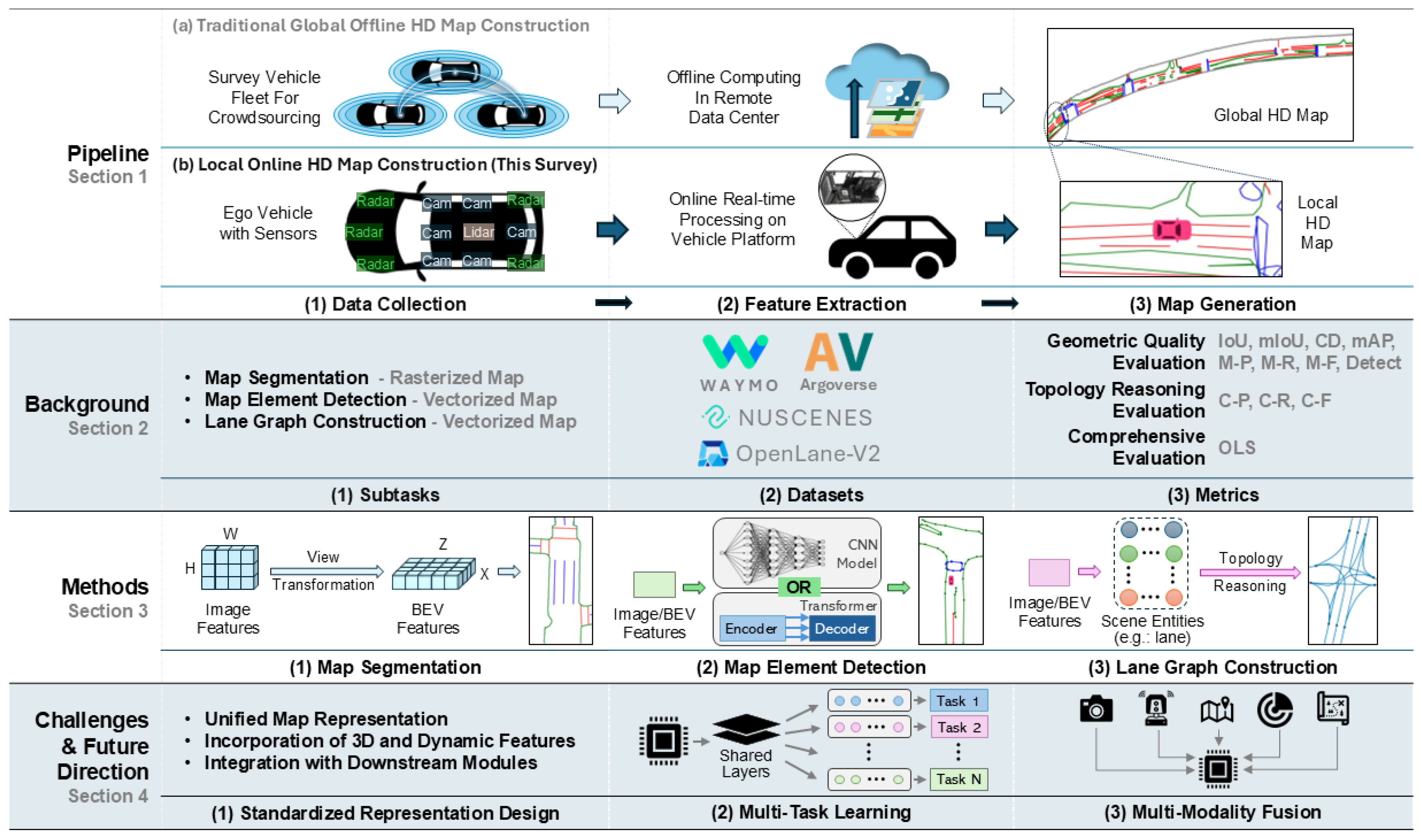
Figure 2.
Comparison of the VT module in two projection-based map segmentation methods.
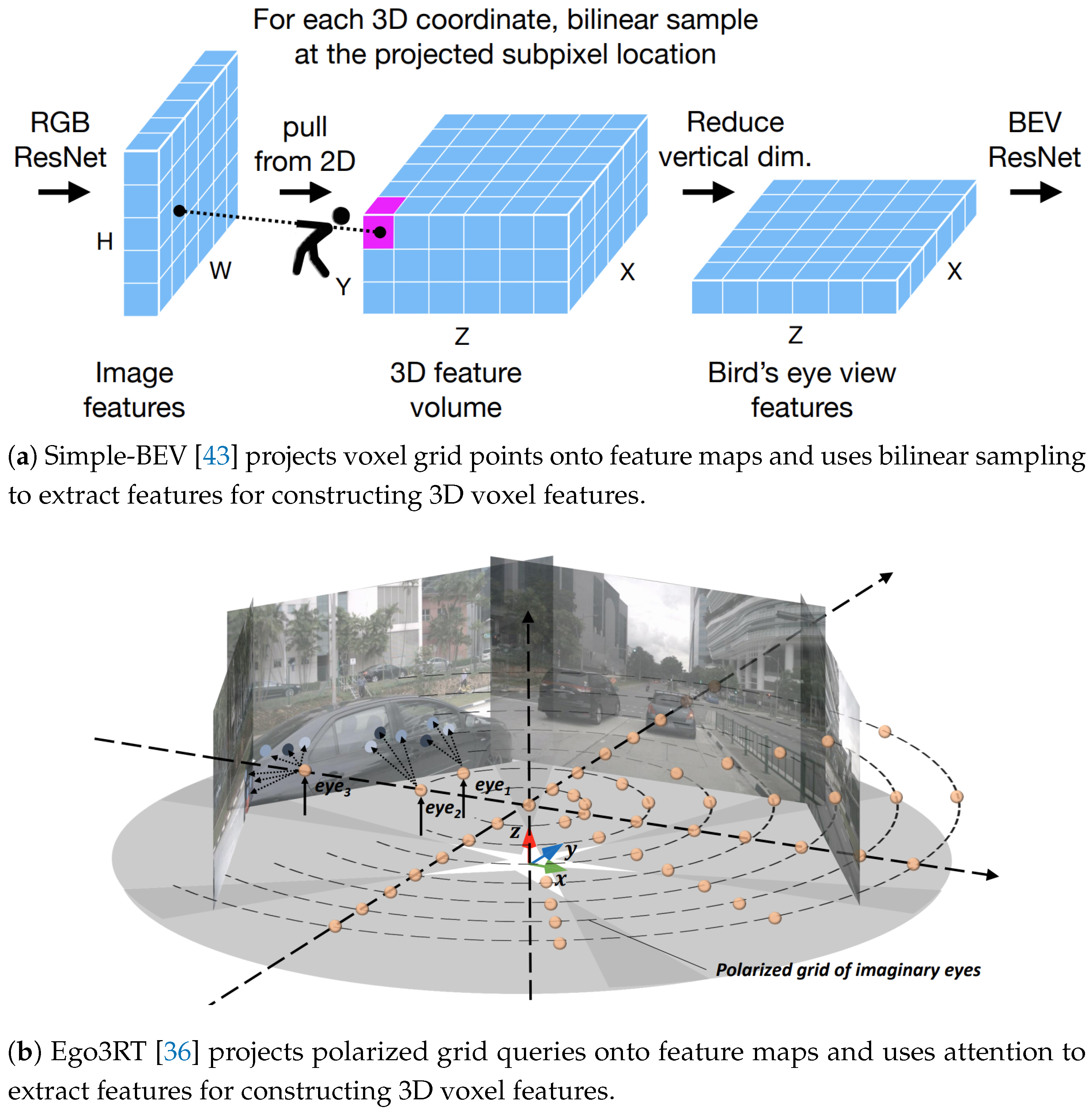
Figure 3.
Comparison of the VT module in two lift-based map segmentation methods.
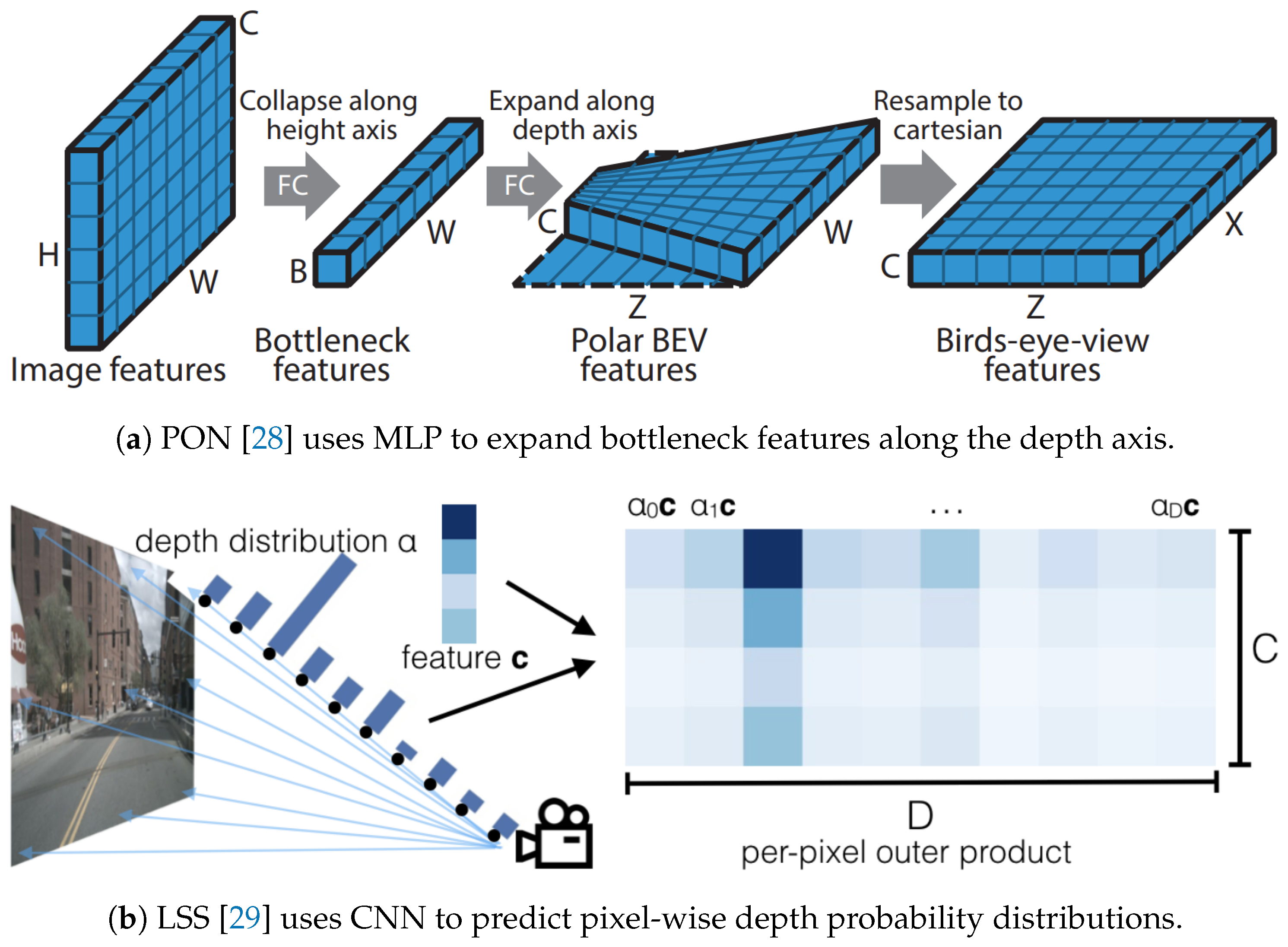
Figure 4.
Comparison of the VT module in two network-based map segmentation methods.
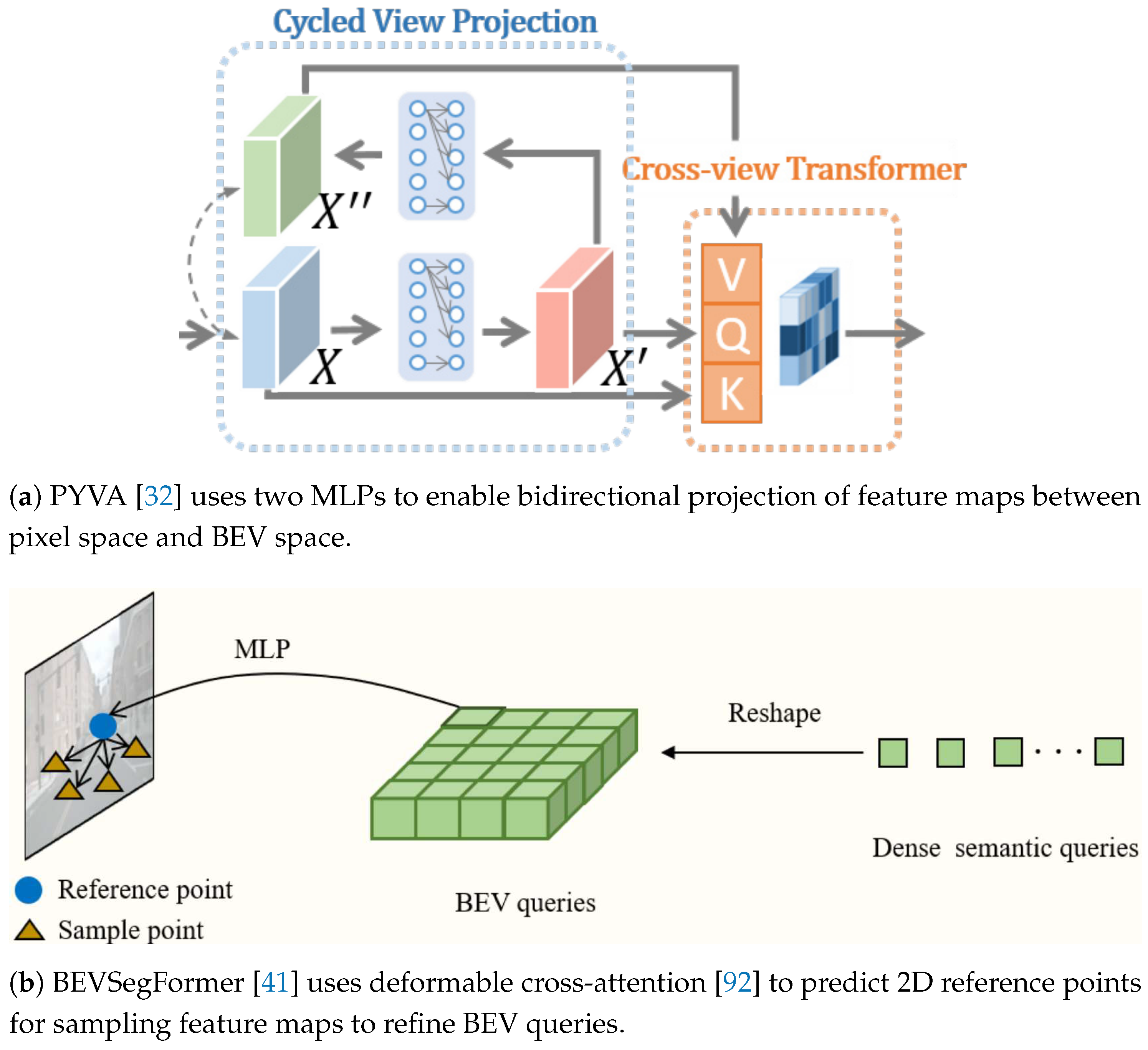
Figure 5.
Comparison of the MD module in two CNN-based map element detection methods.
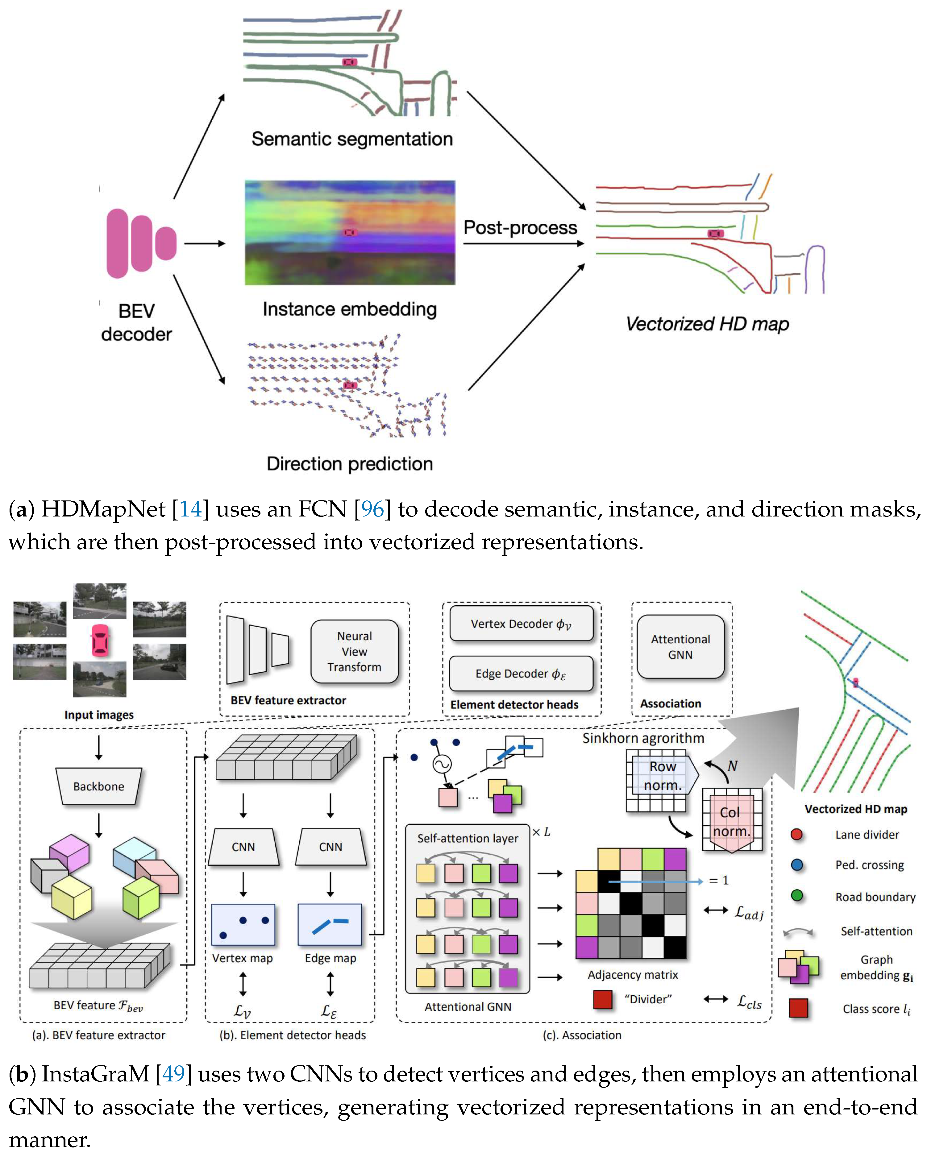
Figure 6.
Comparison of the pipelines of two Transformer-based map element detection methods.
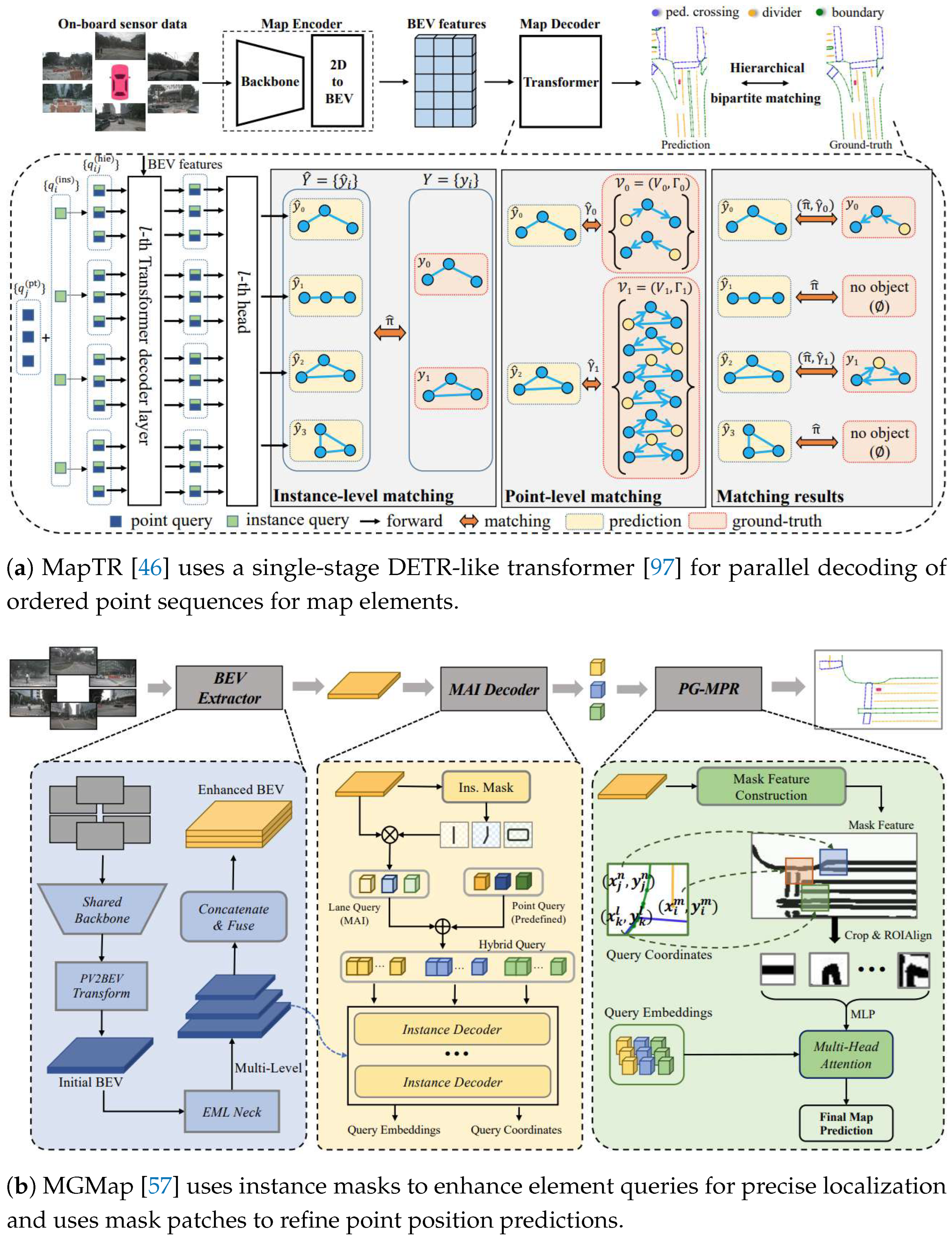
Figure 7.
Comparison of temporal fusion (short-term and long-term) in two Transformer-based map element detection methods.
Figure 7.
Comparison of temporal fusion (short-term and long-term) in two Transformer-based map element detection methods.
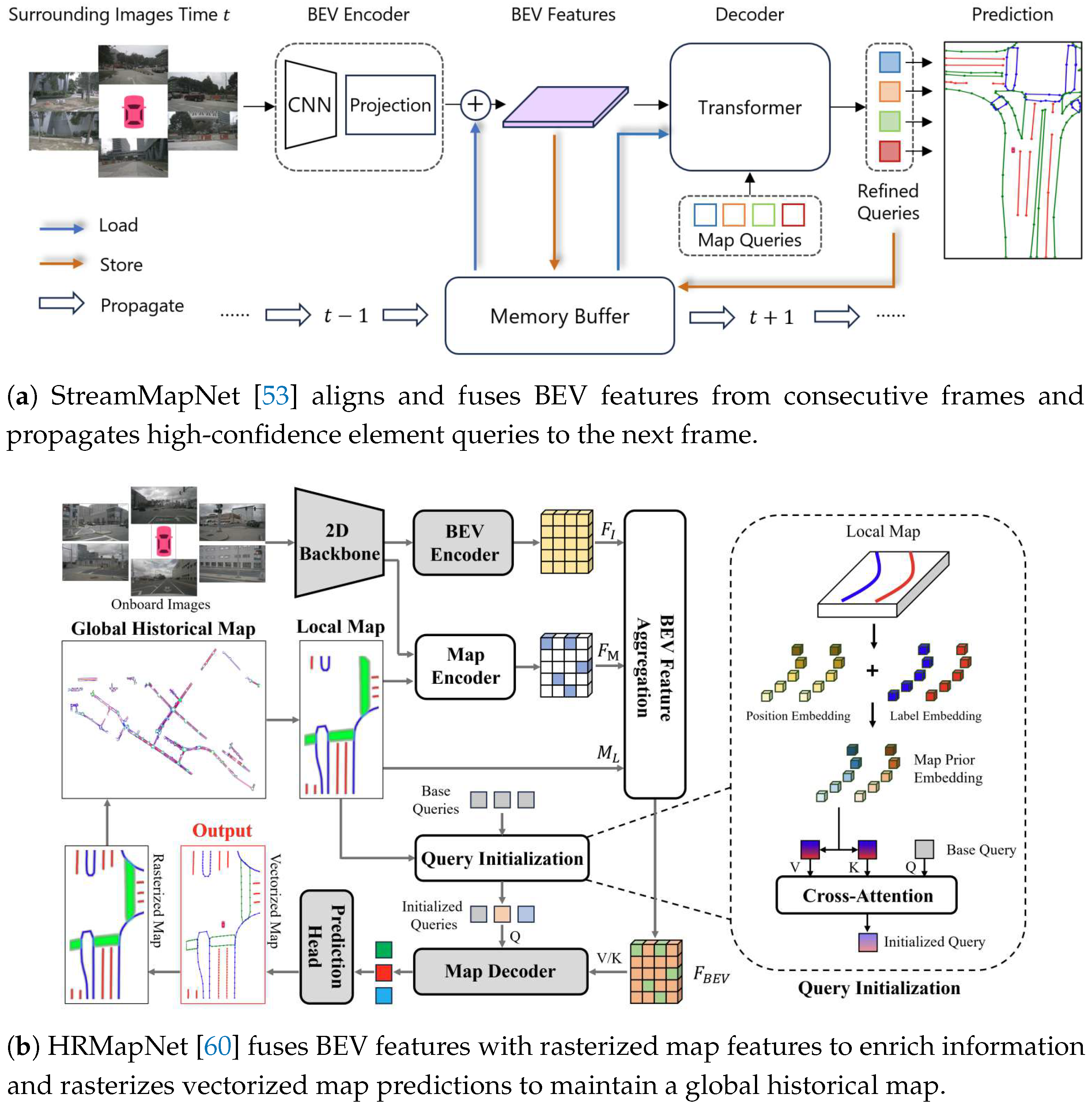
Figure 8.
Comparison of the pipelines for two single-step-based lane graph construction methods.

Figure 9.
Comparison of the TR module in two iteration-based lane graph construction methods.
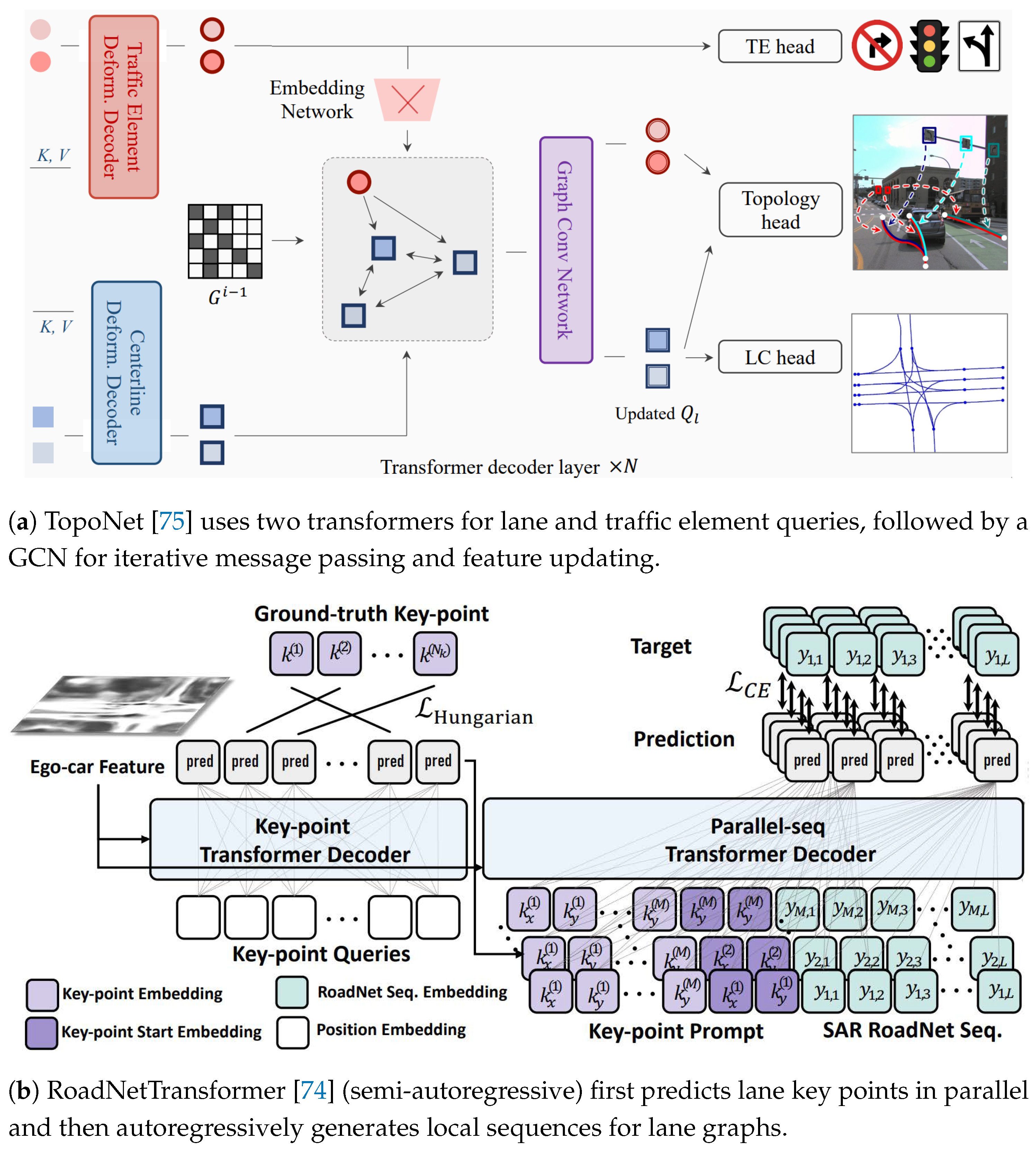
Figure 10.
Comparison of lane segment representation [76] with two alternative map representations.
Figure 10.
Comparison of lane segment representation [76] with two alternative map representations.
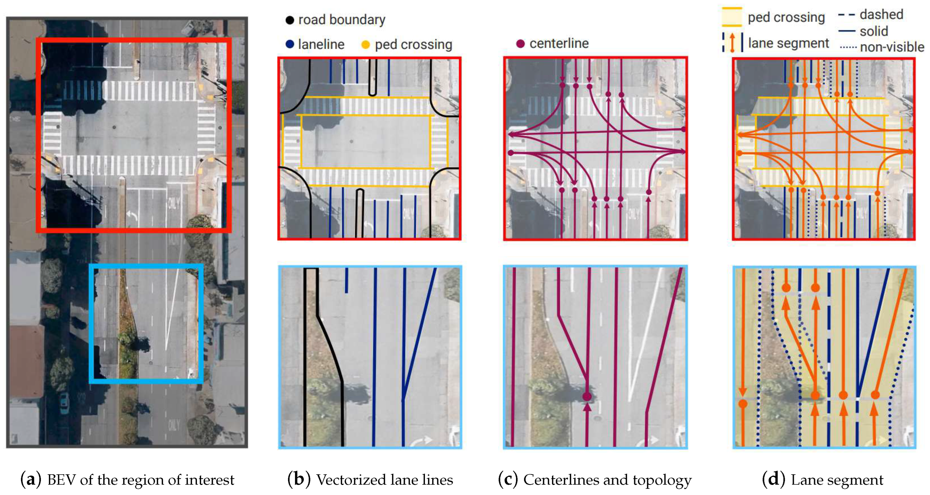
Figure 11.
Comparison of uncertainty-based map representations [103] integrated into various online HD map construction methods.
Figure 11.
Comparison of uncertainty-based map representations [103] integrated into various online HD map construction methods.
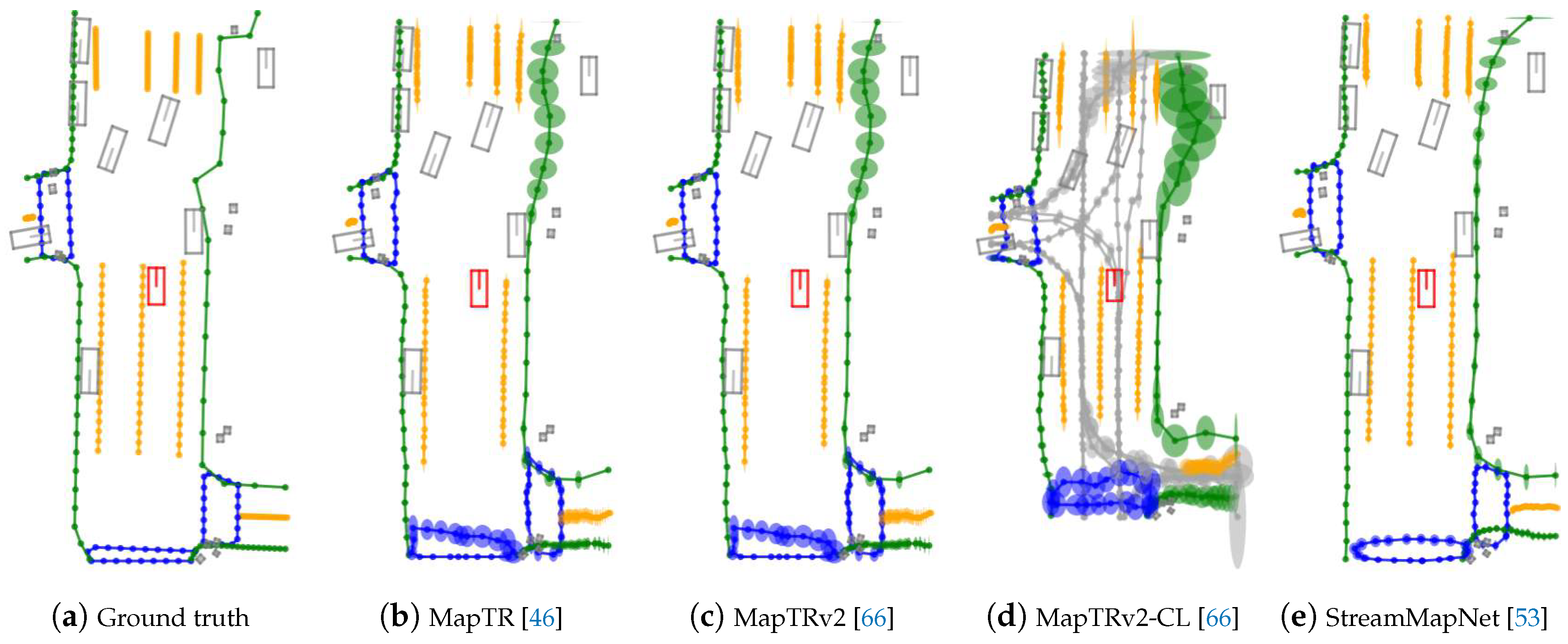
Figure 12.
Comparison of the MTL pipeline in two online HD map construction methods.
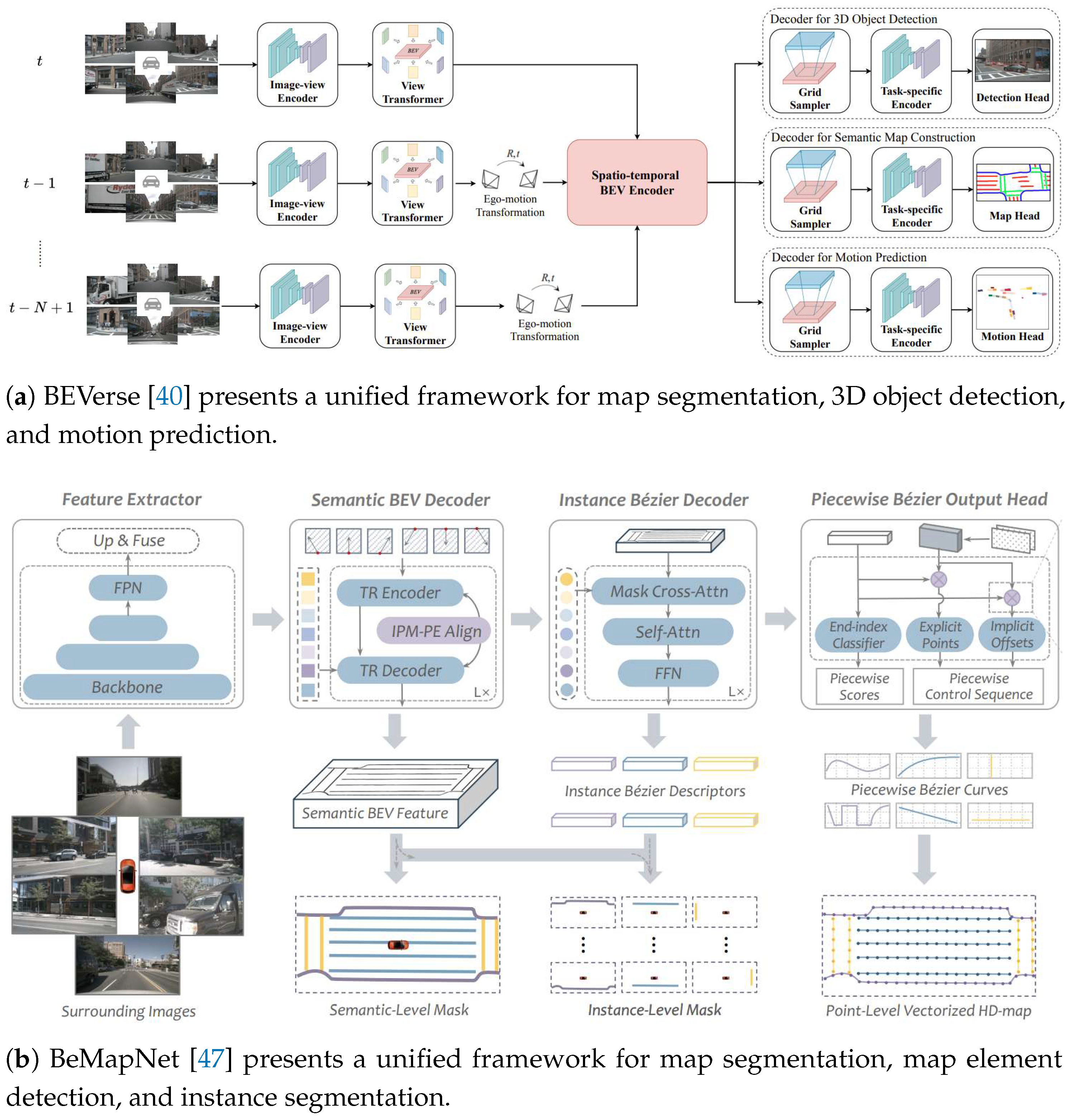
Figure 13.
Comparison of the MMF pipeline in two online HD map construction methods.
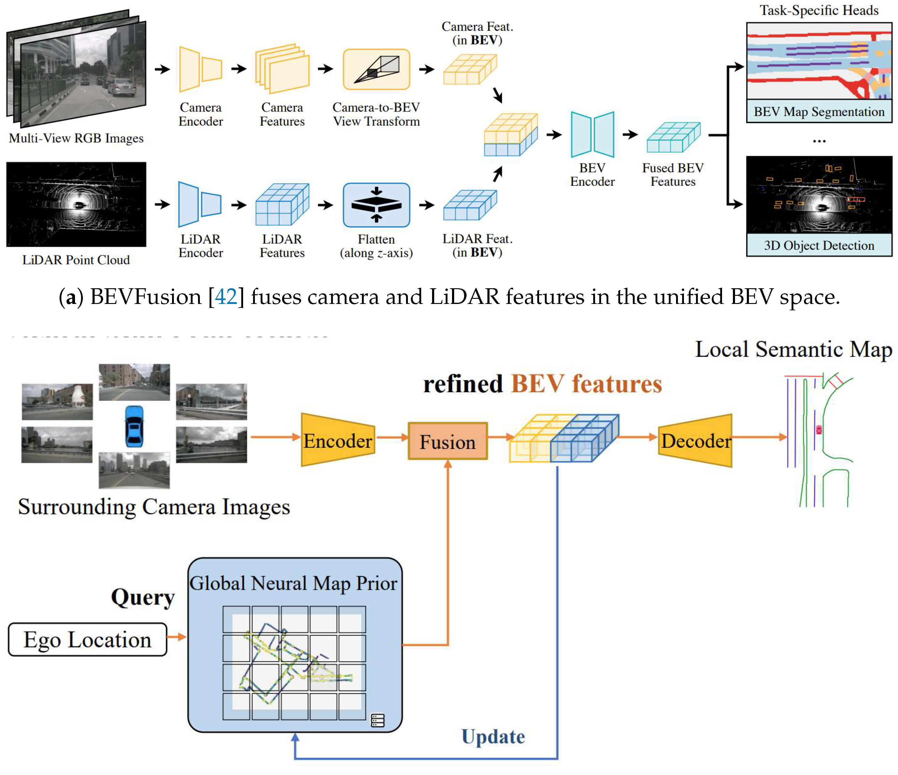

Table 1.
Datasets for Online HD Map Construction. Under Region, "AS" for Asia, and "NA" for North America. Under Data, "# Scenes" refers to the number of dataset splits, and "# Scans" represents the number of point clouds. Under Map Annotation, "# Layers" indicates the number of map semantic layers, and "3D" indicates whether the map is represented in 3D format. The symbol "–" denotes that the statistic is unavailable.
| Dataset | Year | Region | Sensor Data | Map Annotation | |||||
|---|---|---|---|---|---|---|---|---|---|
| # Scenes | # Images | # Scans | # Cities | # Layers | Resolution | 3D | |||
| Waymo [19] | 2019 | NA | 1,150 | 12M | 230k | 6 | 7 | – | 55 |
| NuScenes [20] | 2019 | NA/AS | 1000 | 1.4M | 390k | 2 | 11 | 10px/m | 55 |
| Argoverse 1 [21] | 2019 | NA | 113 | 490k | 22k | 2 | 3 | – | |
| Argoverse 2 [22] | 2023 | NA | 1000 | 2.7M | 150k | 6 | 4 | 100px/m | |
| OpenLane-V2 [23] | 2023 | NA/AS | 2000 | 466K | – | 8 | 3 | – | |
Table 2.
Literature on online HD map construction. Under Modality, "SC" for single-camera, "MC" for multi-camera, and "L" for LiDAR. Under Task, "MapSeg" for map segmentation, "MapEle" for map element detection, and "LaneGra" for lane graph construction. Under Dataset, "nuS" for nuScenes [20], "AV" for Argoverse [21], "K360" for Kitti-360 [27], "AV" for Argoverse 2 [22], and "OL2" for OpenLane-V2 [23].
| Method | Venue | Modality | Task | Dataset | Contribution |
|---|---|---|---|---|---|
| PON [28] | CVPR 2020 | SC | MapSeg | nuS/AV | MLP for Depth Axis Expansion |
| LSS [29] | ECCV 2020 | MC | MapSeg | nuS | CNN for Pixel-Wise Depth Prediction |
| Cam2BEV [30] | ITSC 2020 | MC | MapSeg | Synthetic | IPM for VT on 2D Feature Maps |
| VPN [31] | RA-L 2020 | MC | MapSeg | Synthetic | MLP to Learn Projection for VT |
| PYVA [32] | CVPR 2021 | SC | MapSeg | AV | Cycled View Projection for VT |
| STA-ST [33] | ICRA 2021 | SC | MapSeg | nuS | Temporal Fusion after VT |
| CVT [34] | CVPR 2022 | MC | MapSeg | nuS | Camera-aware Embedding to Enhance VT |
| BEVFormer [35] | ECCV 2022 | MC | MapSeg | nuS | Transformer and Projection for VT |
| Ego3RT [36] | ECCV 2022 | MC | MapSeg | nuS | Ego 3D Representation to Enhance VT |
| LaRa [37] | CoRL 2022 | MC | MapSeg | nuS | Ray Embedding to Enhance VT |
| PanopticSeg [38] | RA-L 2022 | SC | MapSeg | nuS/K360 | Hybrid VT with IPM and Depth Expansion |
| MBEV [39] | arXiv 2022 | MC | MapSeg | nuS | 3D Voxel Grid Projected onto 2D Features |
| BEVerse [40] | arXiv 2022 | MC | MapSeg | nuS | Spatio-temporal Fusion after VT |
| BEVSegFormer [41] | WACV 2023 | MC | MapSeg | nuS | Transformer to Learn Projection for VT |
| BEVFusion [42] | ICRA 2023 | MC/L | MapSeg | nuS | Camera-Lidar Fusion on BEV after VT |
| Simple-BEV [43] | ICRA 2023 | MC/L/R | MapSeg | nuS | Bilinear Sampling for Voxel Quality |
| HFT [44] | ICRA 2023 | SC | MapSeg | nuS/AV | Mutual Learning to Enhance Hybrid VT |
| PETRv2 [45] | ICCV 2023 | MC | MapSeg | nuS | 3D Position Embedding to Enhance VT |
| HDMapNet [14] | ICRA 2022 | MC/L | MapEle | nuS | FCN with Post-processing for MD |
| VectorMapNet [15] | ICML 2023 | MC/L | MapEle | nuS/AV2 | Transformer for Vectorized MD |
| MapTR [46] | ICLR 2023 | MC | MapEle | nuS | Single-stage Transformer for Parallel MD |
| BeMapNet [47] | CVPR 2023 | MC | MapEle | nuS | Piecewise Bezier Curve for MD |
| NMP [48] | CVPR 2023 | MC | MapEle | nuS | Global Neural Map Prior for MD |
| InstaGraM [49] | CVPRW 2023 | MC | MapEle | nuS | CNNs and GNN for Graph-based MD |
| PivotNet [50] | ICCV 2023 | MC | MapEle | nuS/AV2 | Pivot-based Representation for MD |
| ScalableMap [51] | CoRL 2023 | MC | MapEle | nuS | Hierarchical Sparse Map Representation |
| MapVR [52] | NeurIPS 2023 | MC/L | MapEle | nuS/AV2 | Rasterization for Geometric Supervision |
| StreamMapNet [53] | WACV 2024 | MC | MapEle | nuS/AV2 | Streaming Temporal Fusion for MD |
| DPFormer [54] | AAAI 2024 | MC | MapEle | nuS | Douglas-Peucker Point Representation |
| SuperFusion [55] | ICRA 2024 | MC/L | MapEle | nuS | Multi-level LiDAR-camera Fusion for MD |
| HIMap [56] | CVPR 2024 | MC | MapEle | nuS/AV2 | Integrated HIQuery for MD |
| MGMap [57] | CVPR 2024 | MC/L | MapEle | nuS/AV2 | Mask-Guided Learning for MD |
| InsMapper [58] | ECCV 2024 | MC/L | MapEle | nuS/AV2 | Inner-instance Information for MD |
| GeMap [59] | ECCV 2024 | MC | MapEle | nuS/AV2 | Geometric Invariant Representation |
| HRMapNet [60] | ECCV 2024 | MC | MapEle | nuS/AV2 | Global Historical Rasterized Map for MD |
| MapDistill [61] | ECCV 2024 | MC | MapEle | nuS | Cross-modal Knowledge Distillation |
| SQD-MapNet [62] | ECCV 2024 | MC | MapEle | nuS/AV2 | Stream Query Denoising for Consistency |
| MapTracker [63] | ECCV 2024 | MC | MapEle | nuS/AV2 | Strided Memory Fusion for MD |
| ADMap [64] | ECCV 2024 | MC/L | MapEle | nuS/AV2 | Anti-disturbance MD Framework |
| MapQR [65] | ECCV 2024 | MC | MapEle | nuS/AV2 | Scatter-and-Gather Query for MD |
| MapTRv2 [66] | IJCV 2024 | MC/L | MapEle | nuS/AV2 | Advanced Baseline Method for MD |
| DTCLMapper [67] | T-ITS 2024 | MC | MapEle | nuS/AV2 | Dual-stream Temporal Consistency Learning |
| P-MapNet [68] | RA-L 2024 | MC/L | MapEle | nuS/AV2 | SD and HD Map Priors for MD |
| PrevPredMap [69] | WACV 2025 | MC | MapEle | nuS/AV2 | Temporal Fusion with Previous Predictions |
| STSU [12] | ICCV 2021 | SC | LaneGra | nuS | MLP to Infer Lane Connectivity |
| TPLR [13] | CVPR 2022 | SC | LaneGra | nuS/AV | Minimal Cycles for Lane Graph Topology |
| CenterLineDet [70] | ICRA 2023 | MC | LaneGra | nuS | Transformer for Iterative TR |
| VideoLane [71] | ITSC 2023 | SC | LaneGra | nuS/AV | Temporal Aggregation to Enhance TR |
| LaneWAE [72] | ITSC 2023 | SC | LaneGra | nuS/AV | Dataset Prior Distribution to Enhance TR |
| ObjectLane [73] | ICCV 2023 | SC | LaneGra | nuS/AV | Object-Lane Clustering to Enhance TR |
| RoadNetTransformer [74] | ICCV 2023 | MC | LaneGra | nuS | RoadNet Sequence Representation for TR |
| TopoNet [75] | arXiv 2023 | MC | LaneGra | OL2 | GNN to Refine Lane Graph Topology |
| LaneGraph2Seq [26] | AAAI 2024 | MC | LaneGra | nuS/AV2 | Graph Sequence Representation for TR |
| LaneSegNet [76] | ICLR 2024 | MC | LaneGra | OL2 | Lane Segment Representation for TR |
| TopoMLP [77] | ICLR 2024 | MC | LaneGra | OL2 | Robust Detectors to Enhance TR |
| SMERF [78] | ICRA 2024 | MC | LaneGra | OL2 | SD Maps to Enhance TR |
| LaneMapNet [79] | IV 2024 | MC | LaneGra | nuS | Curve Region-aware Attention |
| LaneGAP [80] | ECCV 2024 | MC | LaneGra | nuS/AV2/OL2 | Post-processing to Restore Lane Topology |
| CGNet [81] | ECCV 2024 | MC | LaneGra | nuS/AV2 | GNN and GRU to Optimize Lane Graph |
| TopoLogic [82] | NeurIPS 2024 | MC | LaneGra | OL2 | Lane Geometry and Query Similarity for TR |
| TopoMaskV2 [83] | arXiv 2024 | MC | LaneGra | OL2 | Mask-based Formulation to Enhance TR |
| RoadPainter [84] | arXiv 2024 | MC | LaneGra | OL2 | Points-mask Optimization |
Table 3.
Performance comparison of map segmentation methods on the nuScenes [20] validation set. Under Modality, "SC" for single-camera, "MC" for multi-camera, and "L" for LiDAR. Under VT Type, "Projection," "Lift," and "Network" denote three types of map segmentation methods based on view transformation techniques. The symbol * indicates results from [33], † denotes results from [42], and "–" denotes that the statistic is unavailable.
| Method | Modality | VT Type | Drivable | Ped. Cross. | Walkway | Stop Line | Carpark | Divider | mIoU |
|---|---|---|---|---|---|---|---|---|---|
| VED* [94] | SC | Network | 54.7 | 12.0 | 20.7 | – | 13.5 | – | 25.2 |
| VPN* [31] | SC | Network | 58.0 | 27.3 | 29.4 | – | 12.3 | – | 31.8 |
| PON* [28] | SC | Lift | 60.4 | 28.0 | 31.0 | – | 18.4 | – | 34.5 |
| STA-ST* [33] | SC | Lift | 71.1 | 31.5 | 32.0 | – | 28.0 | – | 40.7 |
| CVT† [34] | MC | Network | 74.3 | 36.8 | 39.9 | 25.8 | 35.0 | 29.4 | 40.2 |
| OFT† [95] | MC | Projection | 74.0 | 35.3 | 45.9 | 27.5 | 35.9 | 33.9 | 42.1 |
| LSS† [29] | MC | Lift | 75.4 | 38.8 | 46.3 | 30.3 | 39.1 | 36.5 | 44.4 |
| MBEV† [39] | MC | Projection | 77.2 | – | – | – | – | 40.5 | – |
| BEVFusion† [42] | MC | Lift | 81.7 | 54.8 | 58.4 | 47.4 | 50.7 | 46.4 | 56.6 |
| BEVFusion† [42] | MC & L | Lift | 85.5 | 60.5 | 67.6 | 52.0 | 57.0 | 53.7 | 62.7 |
Table 4.
Performance comparison of map element detection methods on the nuScenes [20] validation set. Under Backbone, "EB0" for EfficientNet-B0 [98], "R50" for ResNet-50 [99], "PP" for PointPillars [100], and "Sec" for SECOND [101]. Under Modality, "MC" for multi-camera and "L" for LiDAR. Under MD Type, "CNN" and "Transformer" denote two types of map element detection methods based on map decoding techniques. The symbol * indicates results from original papers, and † denotes results from [46].
| Method | Backbone | Epochs | Modality | MD Type | AP | AP | AP | mAP |
|---|---|---|---|---|---|---|---|---|
| HDMapNet† [14] | EB0 | 30 | MC | CNN | 14.4 | 21.7 | 33.0 | 23.0 |
| InstaGraM* [49] | EB0 | 30 | MC | CNN | 40.8 | 30.0 | 39.2 | 36.7 |
| InsMapper* [58] | R50 | 24 | MC | Transformer | 44.4 | 53.4 | 52.8 | 48.3 |
| MapTR* [46] | R50 | 24 | MC | Transformer | 46.3 | 51.5 | 53.1 | 50.3 |
| MapVR* [52] | R50 | 24 | MC | Transformer | 47.7 | 54.4 | 51.4 | 51.2 |
| PivotNet* [50] | R50 | 30 | MC | Transformer | 53.8 | 55.8 | 59.6 | 57.4 |
| BeMapNet* [47] | R50 | 30 | MC | Transformer | 57.7 | 62.3 | 59.4 | 59.8 |
| MapTRv2* [66] | R50 | 24 | MC | Transformer | 59.8 | 62.4 | 62.4 | 61.5 |
| ADMap* [64] | R50 | 24 | MC | Transformer | 63.5 | 61.9 | 63.3 | 62.9 |
| SQD-MapNet* [62] | R50 | 24 | MC | Transformer | 63.0 | 62.5 | 63.3 | 63.9 |
| MGMap* [57] | R50 | 30 | MC | Transformer | 61.8 | 65.0 | 67.5 | 64.8 |
| MapQR* [65] | R50 | 30 | MC | Transformer | 63.4 | 68.0 | 67.7 | 66.4 |
| HIMap* [56] | R50 | 30 | MC | Transformer | 62.6 | 68.4 | 69.1 | 66.7 |
| HDMapNet† [14] | EB0 & PP | 30 | MC & L | CNN | 16.3 | 29.6 | 46.7 | 31.0 |
| InsMapper* [58] | R50 & Sec | 24 | MC & L | Transformer | 56.0 | 63.4 | 71.6 | 61.0 |
| MapVR* [52] | R50 & Sec | 24 | MC & L | Transformer | 60.4 | 62.7 | 67.2 | 63.5 |
| MapTRv2* [66] | R50 & Sec | 24 | MC & L | Transformer | 65.6 | 66.5 | 74.8 | 69.0 |
| ADMap* [64] | R50 & Sec | 24 | MC & L | Transformer | 69.0 | 68.0 | 75.2 | 70.8 |
| MGMap* [57] | R50 & Sec | 24 | MC & L | Transformer | 67.7 | 71.1 | 76.2 | 71.7 |
Table 5.
Performance comparison of lane graph construction methods on the nuScenes [20] validation set (PON [28] split). Under TR Type, "Single-step" and "Iteration" denote two types of lane graph construction methods based on topology reasoning techniques. The symbol * indicates results from original papers, and "–" denotes that the statistic is unavailable.
| Method | TR Type | M-Prec | M-Recall | M-F-score | Detect | C-Prec | C-Recall | C-F-score |
|---|---|---|---|---|---|---|---|---|
| STSU* [12] | Single-step | 60.7 | 54.7 | 57.5 | 60.6 | 60.5 | 52.2 | 56.0 |
| TPLR* [13] | Single-step | – | – | 58.2 | 60.2 | – | – | 55.3 |
| ObjectLane* [73] | Single-step | – | – | 64.2 | 70.6 | – | – | 57.2 |
| VideoLane* [71] | Single-step | – | – | 59.0 | 60.3 | – | – | 61.7 |
| LaneWAE* [72] | Single-step | – | – | 57.0 | 61.2 | – | – | 62.9 |
| LaneMapNet* [79] | Single-step | 71.5 | 64.8 | 67.9 | – | 63.2 | 62.9 | 63.0 |
| LaneGraph2Seq* [26] | Iteration | 64.6 | 63.7 | 64.1 | 64.5 | 69.4 | 58.0 | 63.2 |
Table 6.
Performance comparison of lane graph construction methods on the OpenLane-V2 [23] dataset (v1.0 metrics). Under TR Type, "Single-step" and "Iteration" denote two types of lane graph construction methods based on topology reasoning techniques. SD Map indicates the use of a standard-definition map. The symbol * indicates results from original papers, and † denotes results reproduced by [75].
| Data | Method | TR Type | SD Map | DET | DET | TOP | TOP | OLS |
|---|---|---|---|---|---|---|---|---|
| subset_A | STSU† [12] | Single-step | ✗ | 12.7 | 43.0 | 0.5 | 15.1 | 25.4 |
| TopoNet* [75] | Iteration | ✗ | 28.5 | 48.1 | 4.1 | 20.8 | 35.6 | |
| TopoMLP* [77] | Single-step | ✗ | 28.3 | 50.0 | 7.2 | 22.8 | 38.2 | |
| RoadPainter* [84] | Single-step | ✗ | 30.7 | 47.7 | 7.9 | 24.3 | 38.9 | |
| TopoLogic* [82] | Iteration | ✗ | 29.9 | 47.2 | 18.6 | 21.5 | 41.6 | |
| TopoMaskV2* [83] | Iteration | ✗ | 34.5 | 53.8 | 10.8 | 20.7 | 41.7 | |
| SMERF* [78] (TopoNet) | Iteration | 33.4 | 48.6 | 7.5 | 23.4 | 39.4 | ||
| RoadPainter* [84] | Single-step | 36.9 | 47.1 | 12.7 | 25.8 | 42.6 | ||
| TopoLogic* [82] | Iteration | 34.4 | 48.3 | 23.4 | 24.4 | 45.1 | ||
| subset_B | STSU† [12] | Single-step | ✗ | 8.2 | 43.9 | 0.0 | 9.4 | 21.2 |
| TopoNet* [75] | Iteration | ✗ | 24.3 | 55.0 | 2.5 | 14.2 | 33.2 | |
| TopoMLP* [77] | Single-step | ✗ | 26.6 | 58.3 | 7.6 | 17.8 | 38.7 | |
| RoadPainter* [84] | Single-step | ✗ | 28.7 | 54.8 | 8.5 | 17.2 | 38.5 | |
| TopoLogic* [82] | Iteration | ✗ | 25.9 | 54.7 | 15.1 | 15.1 | 39.6 | |
| TopoMaskV2* [83] | Iteration | ✗ | 41.6 | 61.1 | 12.4 | 14.2 | 43.9 |
Table 7.
Performance comparison of MTL map segmentation methods on the nuScenes [20] validation set. Under Task Head, "MapSeg" for map segmentation, "ObjDet" for 3D object detection, and "MotPre" for motion prediction. The symbol * indicates results from [33], † denotes results from [17], and "–" denotes that the statistic is unavailable.
| Method | Task Head | Map Segmentation | |||||||||
|---|---|---|---|---|---|---|---|---|---|---|---|
| MapSeg | ObjDet | MotPre | Drivable | Lane | Ped. Cross. | Walkway | Carpark | Divider | Boundary | mIoU | |
| MBEV* [39] | ✗ | ✗ | 77.2 | 40.5 | – | – | – | – | – | 58.9 | |
| MBEV* [39] | ✗ | 75.9 | 38.0 | – | – | – | – | – | 57.0 | ||
| BEVFormer* [35] | ✗ | ✗ | 80.1 | 25.7 | – | – | – | – | – | 52.9 | |
| BEVFormer* [35] | ✗ | 77.5 | 23.9 | – | – | – | – | – | 50.7 | ||
| PETRv2† [45] | ✗ | ✗ | 80.5 | 47.4 | – | – | – | – | – | 64.0 | |
| PETRv2† [45] | ✗ | 79.1 | 44.3 | – | – | – | – | – | 61.7 | ||
| Ego3RT* [36] | ✗ | ✗ | 74.6 | – | 33.0 | 42.6 | 44.1 | 36.6 | – | 46.2 | |
| Ego3RT* [36] | ✗ | 79.6 | – | 48.3 | 52.0 | 50.3 | 47.5 | – | 55.5 | ||
| BEVerse* [40] | ✗ | ✗ | – | – | 44.9 | – | – | 56.1 | 58.7 | 53.2 | |
| BEVerse* [40] | – | – | 39.0 | – | – | 53.2 | 53.9 | 48.7 | |||
Table 8.
Performance comparison of MTL MapTRv2 [66] on the nuScenes [20] validation set. Under Task Head, "MapEle" for map element detection, "DepEst" for depth estimation, "MapSeg" for map segmentation, and "SemSeg" for semantic segmentation. The symbol * indicates results from the original paper.
| Method | Task Head | Map Element Detection | ||||||
|---|---|---|---|---|---|---|---|---|
| MapEle | DepEst | MapSeg | SemSeg | AP | AP | AP | mAP | |
| MapTRv2* [66] | ✗ | ✗ | ✗ | 44.9 | 51.9 | 53.5 | 50.1 | |
| MapTRv2* [66] | ✗ | ✗ | 49.6 | 56.6 | 59.4 | 55.2 | ||
| MapTRv2* [66] | ✗ | 52.1 | 57.6 | 59.9 | 56.5 | |||
| MapTRv2* [66] | 53.2 | 58.1 | 60.0 | 57.1 | ||||
Table 9.
Performance comparison of MMF map element detection methods (prior maps) on the nuScenes [20] validation set. Under Prior Map, "SD Map" for standard-definition map [68], "NMP" for neural map prior [48], and "HRMap" for historical rasterized map [60]. The symbol ‡ indicates results from [68], * denotes results from [48], and † represents results from [60].
| Method | Prior Map | Map Element Detection | |||||
|---|---|---|---|---|---|---|---|
| SD Map | NMP | HRMap | AP | AP | AP | mAP | |
| HDMapNet‡ [14] | ✗ | ✗ | ✗ | 10.3 | 27.7 | 45.2 | 27.7 |
| HDMapNet‡ [14] | ✗ | ✗ | 11.3 | 32.1 | 48.7 | 30.7 | |
| VectorMapNet* [15] | ✗ | ✗ | ✗ | 36.1 | 47.3 | 39.3 | 40.9 |
| VectorMapNet* [15] | ✗ | ✗ | 42.9 | 49.6 | 41.9 | 44.8 | |
| StreamMapNet† [53] | ✗ | ✗ | ✗ | 60.4 | 61.9 | 58.9 | 60.4 |
| StreamMapNet† [53] | ✗ | ✗ | 63.8 | 69.5 | 65.5 | 66.3 | |
| MapTRv2† [66] | ✗ | ✗ | ✗ | 59.8 | 62.4 | 62.4 | 61.5 |
| MapTRv2† [66] | ✗ | ✗ | 65.8 | 67.4 | 68.5 | 67.2 | |
Disclaimer/Publisher’s Note: The statements, opinions and data contained in all publications are solely those of the individual author(s) and contributor(s) and not of MDPI and/or the editor(s). MDPI and/or the editor(s) disclaim responsibility for any injury to people or property resulting from any ideas, methods, instructions or products referred to in the content. |
© 2024 by the authors. Licensee MDPI, Basel, Switzerland. This article is an open access article distributed under the terms and conditions of the Creative Commons Attribution (CC BY) license (http://creativecommons.org/licenses/by/4.0/).
Copyright: This open access article is published under a Creative Commons CC BY 4.0 license, which permit the free download, distribution, and reuse, provided that the author and preprint are cited in any reuse.


