Integrative Analysis of Earth to Space Propagation in the EHF Band

1. Introduction

The main progress in technologies using extremely high frequencies (EHF) [1] increased the development of 5 G and 6 G technologies. The EHF frequency ranges from 30 GHz to 300 GHz, according to the ITU definitions [2]. These frequencies are commonly utilized in communication, remote sensing, and radar technology [3]. The frequency selection affects communication platforms, including satellites and communication stations deployed worldwide, to maintain wireless communication. With the increasing utilization of IoT applications, there is a growing need for expanded frequency ranges [4,5]. The need for point-to-point information transmission capacity is steadily increasing, consequently leading to a reduction in the frequency of bandwidth consumption. The lack of free bandwidth has led to the use of free-frequency domains. This frequency domain is divided into subdomains according to IEEE standards. For example, the Ka-Band starts with a frequency of 26.5 GHz to 40 GHz [6]. Despite the challenges and complexities in the EHF field, its benefits and appeal are worth exploring before implementation [7,8,9]. The most influential challenge arises from selective molecular absorption when electromagnetic waves propagate through the atmosphere [10,11]. In addition, several meteorological and physical conditions affect the signal attenuation in the atmosphere, including cloudiness, humidity, water vapor, ozone, and temperature [12,13]. Cloudiness affects the amount of light reaching the ground by scattering and filtering radiation, stabilizing the temperature. Humidity, the amount of water vapor in the air, affects signal quality through the relative humidity ratio, atmospheric absorption, and condensation. Water vapor, a significant greenhouse gas, absorbs long-wave radiation and affects signal transmission. The ozone in the upper atmosphere absorbs harmful UV radiation and acts as a heat reservoir. The earth’s temperature affects the stability of the atmosphere and the propagation of signals, with higher temperatures increasing the water vapor pressure and affecting the density and absorption characteristics of the air. These factors contribute to variability and decreased signal quality in the atmosphere [4,14,15,16,17].

Table 1. EHF Band Subdomain Definition and Support Frequency Range.

Band Subdomain Definition	Support Frequency Range in GHz
Ka1	26.5-40
Q1	33-50
U1	40-60
V1	40-75
E1	60-90
W1	75-110
F1	90-140
D1	110-160
G1	140-220
WR-042	170-260
WR-032	220-300

¹ Standard Radar Frequency Letter-Band (IEEE Standard 521-1984). ² Rectangular Waveguide Size.

Table 1. EHF Band Subdomain Definition and Support Frequency Range.

Band Subdomain Definition	Support Frequency Range in GHz
Ka1	26.5-40
Q1	33-50
U1	40-60
V1	40-75
E1	60-90
W1	75-110
F1	90-140
D1	110-160
G1	140-220
WR-042	170-260
WR-032	220-300

¹ Standard Radar Frequency Letter-Band (IEEE Standard 521-1984). ² Rectangular Waveguide Size.

This study presents a comprehensive approach to calculating the attenuation of total electromagnetic wave propagation from point to point due to passing through the atmosphere at EHF under clear sky conditions. This calculation aims to consider as many main parameters as possible that affect the signal passing from end to end. A corresponding module exists for each parameter. The unification of these modules through an appropriate algorithm forms a singular module for the computation of attenuation. The approach is based on an integrative model. The sub-models of the advanced model are affected by the location of the measured and the desired distance to be measured. The process is carried out by changing the angle of signal transmission at different distances. The angle of transmission can dramatically affect the measured distance. In addition to the effect of the atmosphere, there is also an inferior factor of FSPL. This factor is influenced primarily by distance and frequency. Its effect is very noticeable with an increase in frequency. An overall scheme of atmospheric declination and FSPL name gives a good indication for selecting frequencies for various IoT uses.

In the last decade, the amount of communication systems working at high frequencies has increased. These communication systems include civilian, research, military, and satellite users. The increase in the number of users is due to the significant advantage of using high frequencies, which quickly offer high data transfer capability. Thanks to these advantages, studies have been carried out, and below are several examples of systems that support EHF: communication systems between ground stations and aircraft deployed around the world, satellite communication systems in geostationary orbits, research systems in Chile that use high frequencies to observe astronomical phenomena, such as the formation of stars and molecular clouds, and the 5G communications in Tokyo, Japan and New York, USA.

There are diverse studies in high-frequency fields that aim to advance humanity technologically and give more work capabilities and flexibility. Below are a number of the main topics that the studies deal with:

• Development of 5G and 6G networks, which use EHF frequencies to increase the rates of data passing through, lower the latency, and thus improve the connectivity that enables the activation of new applications such as autonomous vehicles, smart cities, and cellular communication [1,3,18,19,20].
• Satellite and satellite-based communication using EHF frequencies. High frequencies are used in this area to increase the amount of information passing through and improve the coverage of customer areas [8,21,22]. Radar technology using EHF frequencies allows for better resolution and target identification, which are critical for civilian, medical, and military applications. Research on EHF in medicine has shown that intruders and unwanted infections can be diagnosed more precisely [23,24,25].
• Combining EHF frequencies in remote sensing and earthbound observations has improved the accuracy of weather forecasting and environmental monitoring [26,27,28].
• Studies in the field of cyber show that the EHF field is less accessible and requires more expensive electronic systems that are less available on the market today than the systems for lower frequencies; this frequency field is more secure and complicated to disrupt, which makes it possible to use it for military fields, such as intercepting missiles or tracking drones [29,30].
• Studies in quantum communication show the ability to transmit data in secure channels in EHF [31,32].
• Studies show that using EHF frequencies improves the speed of information transfer and helps financial businesses and banks work more precisely [33,34]. EHF frequencies are used in sensor production to improve chip processing capabilities, accuracy, and component control [35,36].

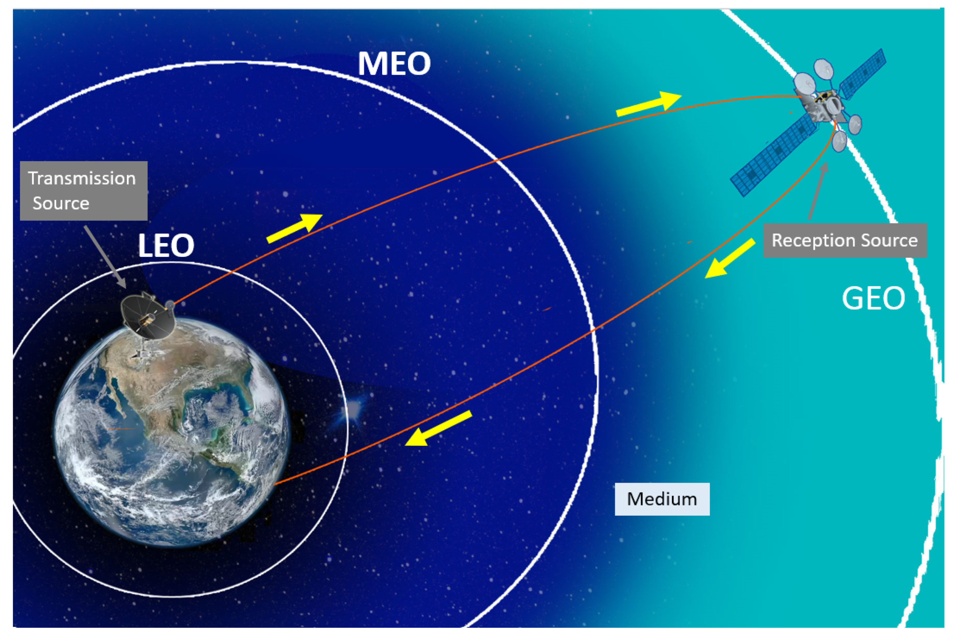
Figure 1. An example of communication between a satellite and a ground station at LEO, MEO, and GEO altitude.

Figure 1. An example of communication between a satellite and a ground station at LEO, MEO, and GEO altitude.

2. Earth to Space MMW Propagation Model

There are several models for calculating atmospheric signal attenuation in the medium due to atmospheric assumption, such as MPM [17], COST [37], and ITU [38]. The model from ITU presented in Recommendation P.676-11 and the model from MPM use the Earth’s atmosphere’s average temperature, atmosphere’s pressure, and water vapor and include the effects of atmospheric humidity, Earth’s curvature, the presence of clouds, and the absorption of radio waves by atmospheric gases. These models also provide a simple way to estimate the radio refractive index for any frequency anywhere [39]. The refractive index $n\left(f\right)$ is frequency-dependent and mainly affected by aerosols [40].

$$n\left(f\right)=1+\underset{\mathrm{N}\left(\mathrm{f}\right)}{\underbrace{[N_0+N^{\prime }\left(f\right)-j{N}^{\prime \prime }\left(f\right)]}}·{10}^{-6}$$

(1)

Where $N\left(f\right)$ (in ppm) is a term of dispersive complex refractivity, $N_0$ is a real and positive constant, $N^{\prime }\left(f\right)$ and $N^{\prime \prime }\left(f\right)$ are the frequency-dependent real and imaginary refractivity terms. By using the transfer function $H\left(jf\right)$ of the atmospheric medium along a distance d, it is possible to represent the real and imaginary parts of refractivity.

$$H\left(jf\right)=\sqrt{T_{FS}\left(d\right)}{e}^{-j{\displaystyle \frac{2\pi f}{c}}·n\left(f\right)d}$$

(2)

Where $T_{FS}\left(d\right)$ is the free-space transmission along a distance d:

$$T_{FS}\left(d\right)=G_R{\left({\displaystyle \frac{c}{2\pi f_c}}\right)}^2{G}_T$$

(3)

Where $G_R$ is the directivity gain of the receiving, and $G_T$ is the directivity gain of transmitting antennas. c is the speed of light in a vacuum, and d is the distance. The transfer function of the atmospheric medium is presented as follows:

$$H\left(jf\right)=\sqrt{T_{FS}\left(d\right)}{e}^{-\left[\alpha \left(f\right)+j\beta \left(f\right)\right]d}$$

(4)

The formulas 2, 3, and 4 show the real and imaginary parts of the atmospheric medium. The imaginary part $\alpha \left(f\right)$ gives the attenuation factor. The second part, $\beta \left(f\right)$, gives the propagating wave number, including phase dispersion.

$$\alpha \left(f\right)={\displaystyle \frac{2\pi f}{c}}{N}^{″}\left(f\right)·{10}^{-6}$$

(5)

$$\beta \left(f\right)={\displaystyle \frac{2\pi f}{c}}+{\displaystyle \frac{2\pi f}{c}}[N_0+N^{\prime }\left(f\right)]{10}^{-6}$$

(6)

The interaction between electromagnetic radiation waves and aerosol molecules induces phenomena of attenuation and phase dispersion electromagnetic waves. The phenomena occur at the frequencies of molecule rotation and vibration [41]. Aerosols are solid and liquid particles in the lower atmosphere, containing minerals such as zinc, iron, and magnesium. Most of the particles come from the land in the weathering processes of soils and rocks and are carried by the wind upwards. The concentration of the particles varies from place to place. Near cities and industrial areas, there is pollution and products of combustion processes, smoke, and soot. In desert areas, there is a high concentration of sand and dust. In a coastal area, there is a high water concentration in different aggregation states and sea salt. In mountainous areas, clear and clean air contains almost no particles. Most are concentrated at low temperatures and vary in size from ${10}^{-3}\mu m$ values. Aerosols are divided into three sterile sizes: Aitken Nuclei - These are particles with a radius smaller than $0.1\mu m$, Large Nuclei - these are particles without a radius of 0.1 $\mu m$ to 1 $\mu m$, and Giant Nuclei - are particles with a radius larger than 1 $\mu m$ [42]. In addition to aerosols, the emitted sun radiation damages the atmospheric layer. The atmosphere is affected by some of this radiation and undergoes significant changes due to the absorption and scattering of the particles. The rest of the radiation is scattered before reaching the ground and is partly reflected, thus heating the Earth where the absorption and diffusion processes are independent [43]. Another noticeable effect is the resonance frequency of a molecule - the frequency at which the molecule absorbs electromagnetic radiation most efficiently. Resonance frequencies are frequencies at which the molecule vibrates and rotates. This frequency is determined by the energy difference between two quantum states of the molecule, which can be affected by factors such as the molecule’s size, shape, and composition. The resonance frequency of a molecule can be calculated using quantum mechanics. The energy difference between two energy levels is proportional to the frequency of the electromagnetic radiation that the molecule can absorb. This frequency can be calculated using the formula:

$$f={\displaystyle \frac{\Delta E}{\hslash }}={\displaystyle \frac{\Delta mv}{\hslash }}$$

(7)

Where f is the resonance frequency of the molecule, $\Delta E$ is the energy difference between two quantum states of the molecule, and ℏ is Planck’s constant [44]. Combining effects that affect the signal stability in the medium and integration on the route makes it possible to create a signal stability model that references the overall stability along the entire medium. This model consists of several modules that depend on each other. To calculate the values more accurately, the models are based on a working point on the earth’s surface - the area of Southern Europe. To provide solutions for all scenarios, the model bases the solutions on existing models that allow accurate assessments to be given as much as possible in the shortest possible time. ITU models require providing the following values: atmospheric pressure, water vapor level, and temperature. The three factors vary according to the sampled height above the Earth’s surface, region, and time. The prevailing temperature in the atmosphere and exposure to the sun affect the total calculation. The prevailing temperature in the atmosphere and the exposure to the sun greatly influence the calculation of the total attenuation. As a result, the models are adapted to two situations: for a hot season when the sun is directed towards the earth (for example, summer, noon) and a cold season when the sun is not directed towards the area of examination (for example, winter, night).

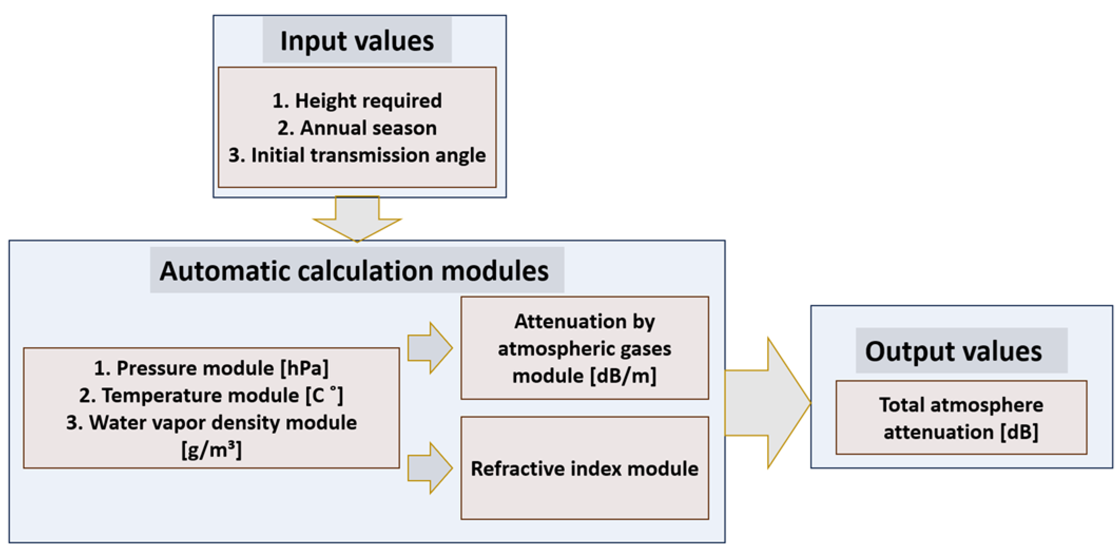
A calculation set of the electromagnetic wave attenuation module consists of modules required for calculating attenuation at any point in space (see Figure 2). With knowledge of attenuation at each point in space, it is possible to add all the attenuation points until reaching the required height in a desired vector and thus obtain the total attenuation on the route. The modules are as follows:

• Temperature module - the purpose of the model is to give an output of the temperature as a function of height in units of Kelvin or Celsius. There are two distributions: for a hot state and a cold state.
• A water vapor model - This gives an output of the amount of water vapor as a function of height in units of $g/m^3$.
• An atmospheric pressure model - This gives an output of atmospheric pressure as a function of height in units of hPa
• A signal refraction angle calculation model that allows accurate planning for the progress of the signals.

At each point of its height, the following values will be obtained: temperature, water vapor level, and atmospheric pressure. These values are fed into the ITU attenuation model, which allows the attenuation value to be given at any desired frequency at any height point (depending on meteorological values). The slope of the route is carried out by the derivative of fixed distances from the total route; each derivative equals 100 meters. To calculate a path that starts from a point of height 0 up to a certain height, the refraction model will be used to find the refraction coefficient. For each change in height of 100 meters, the coefficient will change and adjust itself to the value of the same height; by this change, the angle of refraction will also change. Also, by Snell’s law, the system will calculate the route of the signal. The total attenuation is calculated by the attenuation integral of the transmission route up to its desired height.

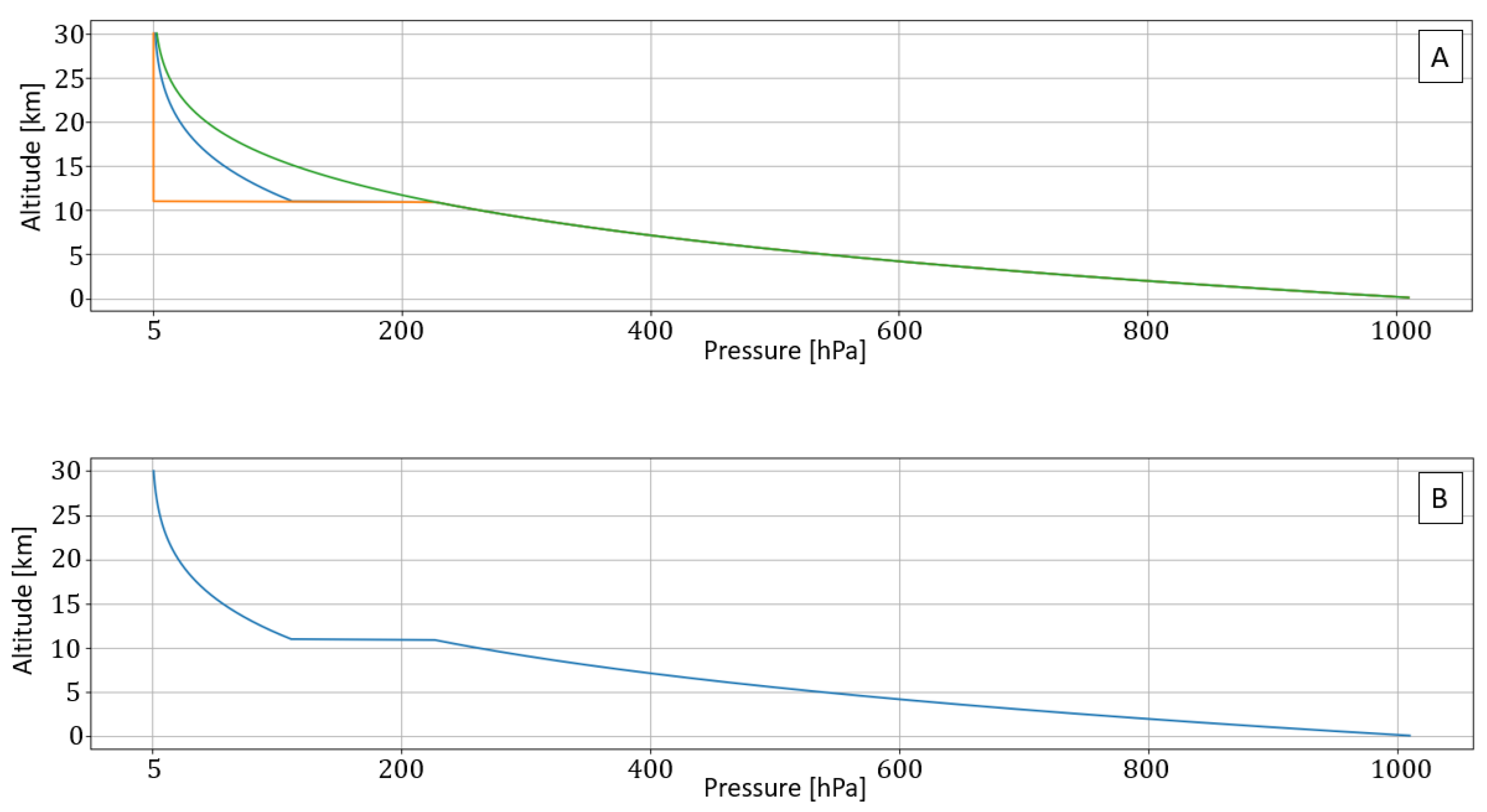
2.1. Pressure Effect

The model is based on an analytical calculation of pressure level as a function of its height. The main assumptions that affect the pressure are the ratio of liquids and gases in the atmosphere gravity, which is affected according to the height and molecular composition of the sampled area. Zero altitudes are measured from the mean sea level on Earth. Mean sea level varies everywhere on the earth’s geodetic ellipsoid and is affected by gravitational potential energy. The model includes the effects of gravitational changes and [45] contributions. The rate of change in temperature is defined as the rate of increase or decrease in temperature in the atmosphere with an increase in altitude. The model refers to a constant state of temperature change. For the model, the assumption is that the rate of change at Zero altitude is -6.5 mK/m. This model allows this rough assumption because up to 11 km, the temperature does not change much. After a height of 11 km, the behavior of the temperature is constant, which reduces the atmospheric pressure at a higher rate. The accuracy in the area above 11 km can be neglected because the pressure level at this height is ten times lower than that on the ground and even tends to 0 [Pa] at an altitude of 13 km. A calculation assumption considers that the gas is constant in air and its behavior is constant. This situation is expected when the molecular composition of the gases in the atmosphere does not change, which is not necessarily true in the polar regions and the equator. According to the theoretical model, the differences in atmospheric pressure as a function of altitude are affected by the molecular density of the air and the force of gravity:

$${\displaystyle \frac{dP}{dz}}=-\rho g$$

(8)

Where P is atmospheric pressure, z is the height above the earth perpendicular to the ground, $\rho$ is the air density, and g is the gravitational acceleration. According to the law of ideal gases:

$$P=\rho RT$$

(9)

Where R is the gas constant in air and T is the temperature. For constant T and g, z can be described by solving a first-order differential equation:

$$z=-{\displaystyle \frac{RT}{g}}Log\left[{\displaystyle \frac{P}{P_0}}\right]$$

(10)

Calculation of pressure level at a desired height point is made possible by an integral of non-linear values of atmospheric pressure level and gravity.:

$$P\left(z\right)=P_{0}exp\left[-{\displaystyle \frac{1}{R}}\left({\int }_0^z{\displaystyle \frac{g\left[\alpha \right]}{T\left[\alpha \right]}}d\alpha \right)\right]$$

(11)

where $\alpha$ is a coefficient for an integral. We will use the temperature change rate L:

$${\displaystyle \frac{G{M}_e}{{\mathrm{R}}_{\left[z\right]}^2}}{\int }_0^z{\displaystyle \frac{d\alpha }{T_0+L\alpha }}={\displaystyle \frac{g}{L}}(log\left[T_0\right]+Lz)-log\left[T_0\right])$$

(12)

Where G is a gravitational constant, $M_e$ is the mass of the Earth, $R_z$ is its height measured according to the center of the Earth, and g is the acceleration of gravity. Below is the solution to the equation for finding the pressure level as a function of its height when $R_z=R_e+z$ :

$$P\left[z\right]=P_0{\left[{\displaystyle \frac{zL+T_0}{T_0}}\right]}^{{\displaystyle \frac{-G{M}_e}{LR{\left(R_{e+z}\right)}^2}}}$$

(13)

Table 2. Below are the parameters that can be included in the equation to determine the pressure level as a function of height above the earth:

Sign	Description of the value	Value	Units
$P_0$	Pressure level at zero altitude1	101325	$P_a$
$T_0$	Temperature at zero altitude1	288.15	K
g	Gravity acceleration at zero altitude1	9.80665	$m/s^2$
L	Rate of temperature change in the troposphere1	-6.5	$K^0/km$
R	Universal gas constant1	287.053	$J/kg·$$K^0$
G	Gravitational constant1	$6.674·$${10}^{-11}$	$m^3/kg·s^2$
$M_e$	Earth’s mass1	$5.972·$${10}^{24}$	Kg
$R_e$	Earth’s radius1	$6.371·$${10}^6$	meter

¹ The values are contingent on the Earth’s location definition and can differ based on region. However, the disparities are negligible between geographic areas.

Table 2. Below are the parameters that can be included in the equation to determine the pressure level as a function of height above the earth:

Sign	Description of the value	Value	Units
$P_0$	Pressure level at zero altitude1	101325	$P_a$
$T_0$	Temperature at zero altitude1	288.15	K
g	Gravity acceleration at zero altitude1	9.80665	$m/s^2$
L	Rate of temperature change in the troposphere1	-6.5	$K^0/km$
R	Universal gas constant1	287.053	$J/kg·$$K^0$
G	Gravitational constant1	$6.674·$${10}^{-11}$	$m^3/kg·s^2$
$M_e$	Earth’s mass1	$5.972·$${10}^{24}$	Kg
$R_e$	Earth’s radius1	$6.371·$${10}^6$	meter

¹ The values are contingent on the Earth’s location definition and can differ based on region. However, the disparities are negligible between geographic areas.

Depending on the placement of all the values, a function for atmospheric pressure P in hPa units will be:

$$P\left[z\right]=101325{\left[{\displaystyle \frac{z(-0.0065)+288.15}{288.15}}\right]}^{{\displaystyle \frac{-6.674·{10}^{-11}·5.972·{10}^{24}}{-0.0065·287.053·{(6371000+z)}^2}}}$$

(14)

This analysis is valid for a domain up to the tropopause. When an electromagnetic wave passes through the layers above the troposphere, it causes temperature changes. In the tropopause layer, the temperature almost does not change, and as a result, the air pressure decreases in a very sharp exponential gradient.

The graphs are shown in Figure 3, an exponential drop in air pressure levels as a function of altitude. The graphs show an exponential drop in air pressure up to a height of 11 km. After 11 km, the behavior is variable and depends mainly on temperature changes. From theoretical models, it is possible to construct a lower limit - an orange graph and an upper limit - a green graph. It is impossible to be precise in these areas because they depend on the small changes in the spread of air molecules. For a computational model, it is possible to base it on a simple average between the two limits - according to the blue graph.

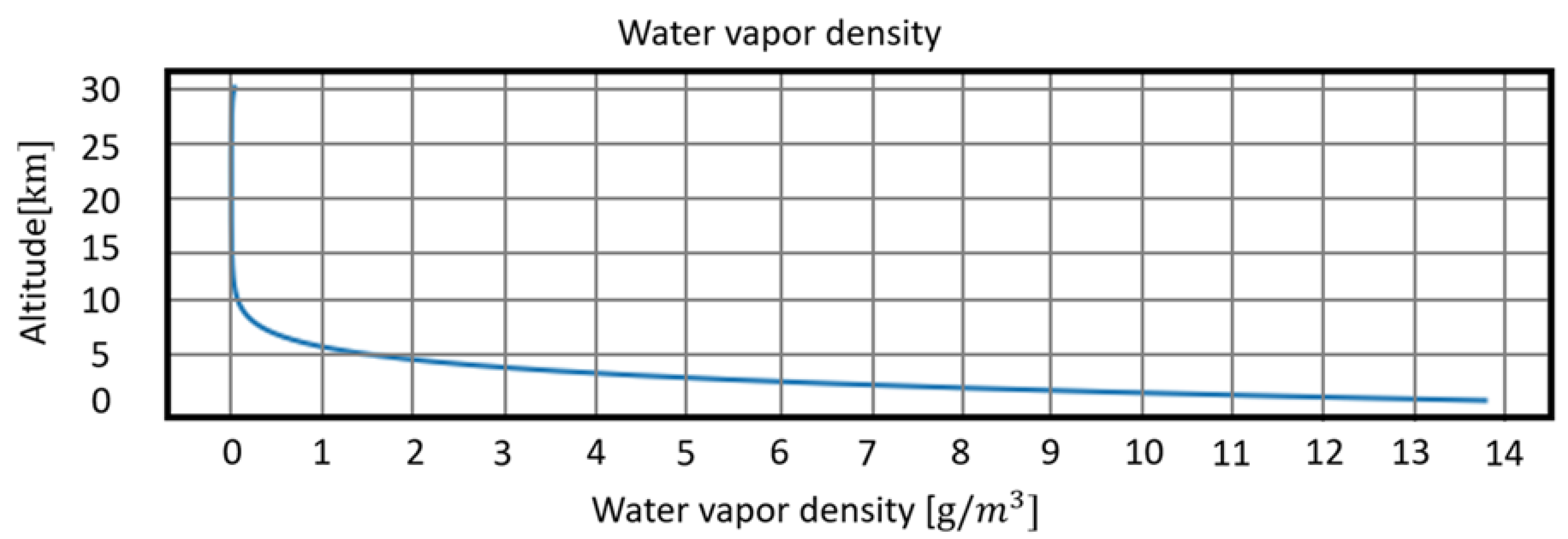
2.2. Water Vapor Effect

The distribution of water vapor in the atmosphere is usually very variable. The influencing parameters are temperature and the pressure level that allow the particles to reach equilibrium. Temperature is greatly affected by altitude, as is atmospheric pressure. The moisture percentage is another critical factor in the equation and is shown directly from the temperature and the processes of dispersion and absorption. Equation 15 shows the ground-level water vapor values at any temperature. At different altitudes, there is a different behavior of the humidity level. To model a simple equation, we can use a basic presentation of a distribution that depends only on its height:

$$\rho \left(h\right)={\rho }_{0}exp\left({\displaystyle \frac{-h}{h_0}}\right)$$

(15)

where ${\rho }_0$ is the water vapor level at height 0. There are several different standards for different locations on Earth in different seasons. According to ITU [46] and geographical considerations, in the model, we will use Equation 16 in the values corresponding to the regions above the equator in the summer seasons, which are very similar to the winter seasons in the equatorial regions:

$$\rho \left(h\right)=14.3542exp(-0.4174h-0.0229h^2+0.0001007h^3)$$

(16)

According to formula 16, a distribution in the land area is equal to 13.76 $g/m^3$. At a height of 100 meters, 9.25 $g/m^3$ is obtained. This value corresponds to the one shown in [47] and thus proves the correctness of the approximate formula.

Figure 4 shows the distribution of water vapor density as a function of height. The value resets after 10 km.

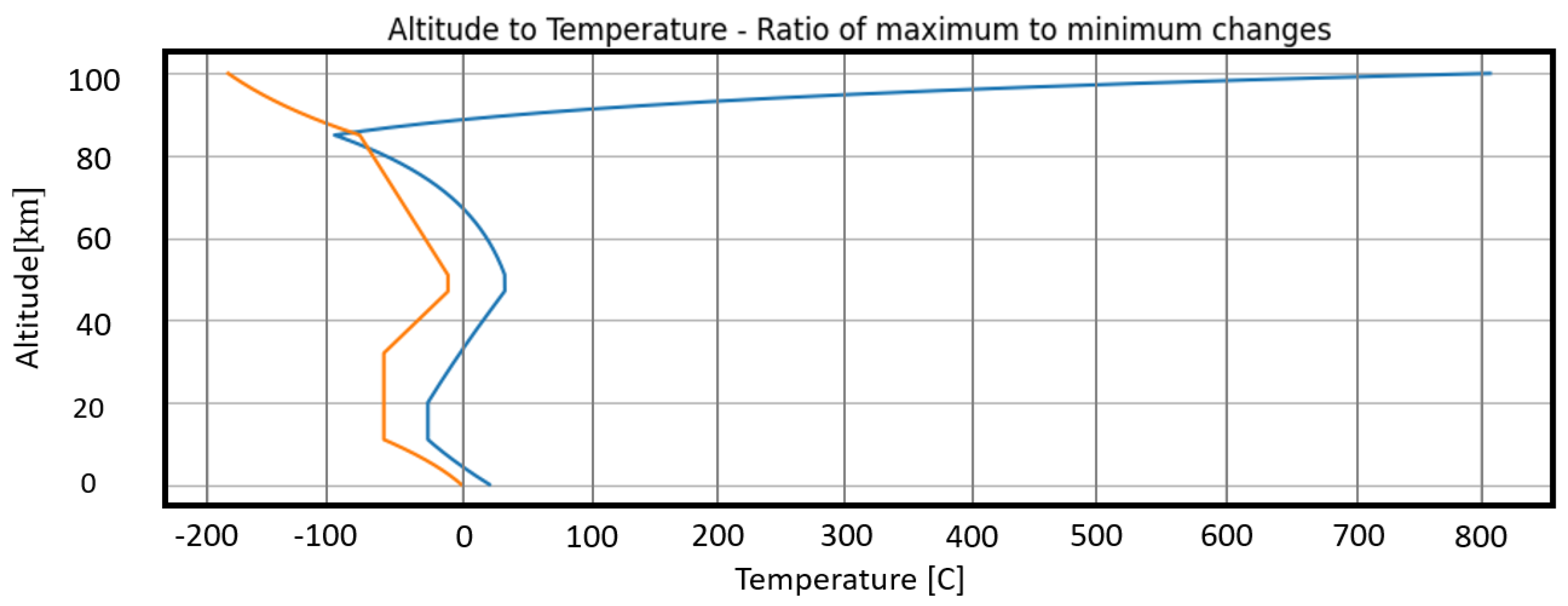
2.3. Temperature Effect

The temperature distribution is a product of air humidity and atmospheric pressure. These two factors determine the location of the spread and the presence of particles that make up the atmosphere. There is a standard that represents the variation of temperature with altitude. The standard’s starting point is 15 degrees Celsius, but it can be changed by determining the location. For Mediterranean areas, there is a zero point of 22 degrees during the day in summer and 0 degrees in winter. At altitudes above 80 km, the temperature depends on the sun’s position in the transmission and reception fields of the signal. Below is a distribution by height-dependent functions [46]:

$$T_{Hot}\left(h\right)=\left\{\begin{array}{c}294.9839-5.2159h+0.07109h^2,for:0\le h\le 11\\ 246.21,for:11\le h\le 20\\ 246.21exp((h-20)8.128·{10}^{-3}),for:20\le h\le 47\\ 306.63,for:47\le h\le 51\\ 306.63+20(1-exp(0.06(h-51)\left)\right),for:51\le h\le 85\\ 172.81·1.{13}^{h-85},for:85\le h\le 36000\end{array}\right.$$

(17)

$T_{Hot}\left(h\right)$ in formula 17 indicates a distribution function of the temperature in Kelvin values in the Mediterranean region on a hot day during the noon. Distance is measured in units of km.

$$T_{Cold}\left(h\right)=\left\{\begin{array}{c}272.7241-3.6217h-0.1759h^2,for:0\le h\le 11\\ 211.601,for:11\le h\le 32\\ 211.601+3.3571(h-32),for:32\le h\le 47\\ 261.958,for:47\le h\le 51\\ 261.958-2.037(h-51),for:51\le h\le 85\\ 192.7·0.{95}^{h-85},for:85\le h\le 36000\end{array}\right.$$

(18)

$T_{Cold}\left(h\right)$ in formula 18 indicates a distribution function of the temperature in Kelvin values in the Mediterranean region on a cold day during the night. Distance is measured in units of km.

In Figure 5, two graphs are shown that are derived for functions 17 and 18. The blue graph depicts temperature behavior as a function of the day during summer. The orange graph depicts the temperature distribution at night during winter. The distribution is adapted to ITU standards according to the geographical location in the Mediterranean.

3. Atmospheric Refraction Effects Model

Refraction index $n\left(f\right)$ determines the intensity of reflection and transmission of an electromagnetic signal and varies according to the atmospheric parameters. Also, it allows the calculation of the medium refraction index $n_r\left(f\right)$. The wave’s propagation angle between different atmospheric levels can be found by using the refraction index and Fresnel equation. This value of the refraction index can be calculated by the formula $\beta \left(f\right)$6. ITU presented a simple calculation method in Recommendation P.453-11 without considering the frequency. This constant depends on temperature, humidity, impurities, and wind speed. Humidity can significantly change the value of $n\left(f\right)$. In severe heat conduction, a phenomenon known as "plumbing" occurs. This phenomenon is manifested in the rise of hot air in the form of giant bubbles, and at the same time, cold air descends between these bubbles to replace the hot air. The temperature changes in the hot areas are more significant than those in the cold regions, and therefore, there are extreme changes in the air temperature. Fluctuations in the refractive index cause fluctuations in the electromagnetic radiation. The refractive index of the atmosphere in radio waves can be calculated by the real domain of the formula $n_r$ [39,48]:

$$n_r\left(f\right)=1+[N_0+N^{\prime }\left(f\right)]·{10}^{-6}$$

(19)

By neglecting frequency propagation effects, a simplified model can be used. Only $N_0$ will be taken into account.

$$n_r=1+77.6{\displaystyle \frac{P_d}{T}}+72{\displaystyle \frac{e}{T}}+3.75·{10}^{-5}{\displaystyle \frac{e}{T^2}}$$

(20)

When e – momentary water vapor pressure [hPa], T – absolute temperature [K], P – total atmospheric pressure [hPa], $P_d$ – dry atmospheric pressure [hPa]. According to the assumption: $P=e+P_d$, a simplification is obtained:

$$n_r=1+77.6{\displaystyle \frac{P}{T}}-5.6{\displaystyle \frac{e}{T}}+3.75·{10}^5{\displaystyle \frac{e}{T^2}}$$

(21)

The water vapor particle pressure e can be obtained using the water vapor density in the air by the following expression:

$$e={\displaystyle \frac{\rho T}{216.7}}$$

(22)

Where $\rho$ is the amount of water vapor in units $g/m^3$. The final function is obtained [49]:

$$n_r=1+77.6{\displaystyle \frac{P}{T}}-5.6{\displaystyle \frac{\rho }{216.7}}+3.75·{10}^5{\displaystyle \frac{\rho }{216.7T}}$$

(23)

4. Cumulative Attenuation

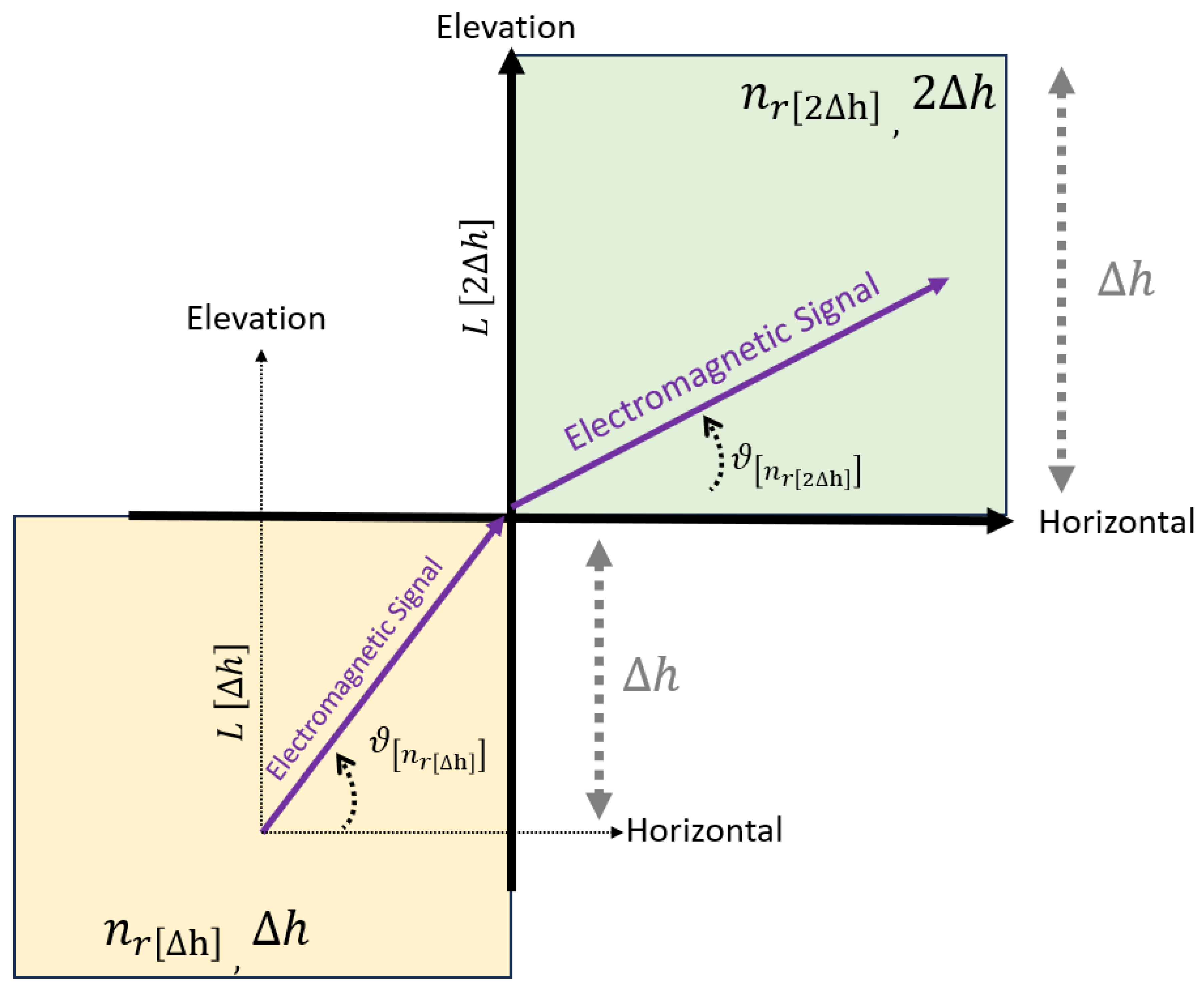
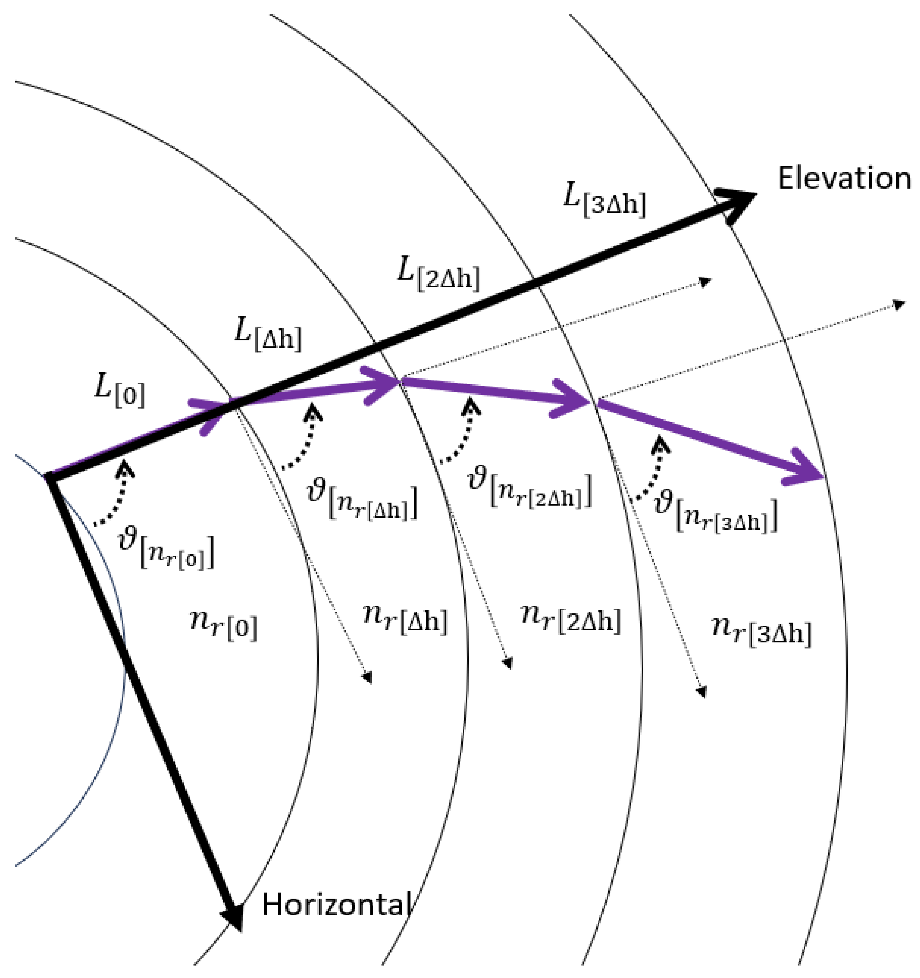
Calculating the overall atmospheric attenuation requires considering every segment of the electromagnetic wave passing through the atmosphere. Each segment has its own attenuation level. The distribution of attenuation levels at every frequency and every point of its height is not linear, nor does it depend on its height itself, but instead on the physical parameters at that height (atmospheric pressure, amount of water vapor, molecular dispersion, etc.). The calculation process is based on a desired height accuracy resolution (ranging from 100 to 1000 meters). In the working resolution, an elevation angle depends on the initial angle as described in Figure 6.

Each segment’s attenuation factors are summed to produce a cumulative attenuation up to the desired point. Where the initial elevation transmission angle is defined as $\vartheta \left[0\right]$ and the initial refraction index $n_{r\left[0\right]}$ and initial elevation attenuation factor $L_0$.Each layer creates its refraction index when passing between many layers in the atmosphere. As a result, each layer will also have its attenuation factor, and the elevation angle $\vartheta \left[n_r\right]$ will change accordingly. Each layer maintains a height accuracy resolution of $\Delta h$.

Cumulative attenuation $L\left(h\right)$ is the sum of all $L_{\Delta nh}$ values. it can be defined as:

$$L\left(h\right)=L_0+L_{\Delta h}+L_{2\Delta h}+L_{3\Delta h}+...+L_{nh}=\sum _{i=0}^n{L}_{nh}$$

(24)

Cumulative attenuation $L\left(h\right)$ can be shown by integrating the values of attenuation factors $L_{\Delta h}$.

$$\mathrm{L}\left[h\right]={\int }_0^h\left({\displaystyle \frac{L\left[h^{\prime }\right]}{sin{\vartheta }_{h^{\prime }}}}\right)d{h}^{\prime }$$

(25)

According to Snell’s law :

$$cos\left[\vartheta \left(h^{\prime }\right)\right]={\displaystyle \frac{n_r\left(0\right)cos\left[\vartheta \left(0\right)\right]}{n_r\left(h^{\prime }\right)}}$$

(26)

Identify the overall atmospheric attenuation value within the obtained range:

$$\mathrm{L}\left[h\right]={\int }_0^h\left({\displaystyle \frac{L\left[h^{\prime }\right]}{\sqrt{1-{\left(\frac{n_r\left(0\right)cos\left[\vartheta \left(0\right)\right]}{n_r\left(h^{\prime }\right)}\right)}^2}}}\right)d{h}^{\prime }$$

(27)

Specific attenuation $L\left(h^{\prime }\right)$ is based on an ITU standard [38]. The main factors that affect the attenuation of an electromagnetic wave in the atmosphere are the water vapor in the air, temperature, and air pressure in the same area. These factors have a univalent effect on the level of humidity and the probability of the different types of gases in the air. There are also different accumulations of gases and humidity levels at certain altitudes. Each segment’s attenuation factor is defined by the function $\alpha \left(f\right)$ (see formula 5).

$$L\left(h^{\prime }\right)[db/m]=20log\left(e\right)\alpha \left(f\right)=20log\left(e\right)·{\displaystyle \frac{2\pi f}{c}}{N}_{\left(f\right)}^{\prime \prime }·{10}^{-6}=1.82·{10}^{-6}f{N}_{\left(f\right)}^{\prime \prime }·{10}^{-6},f\left[Hz\right]$$

(28)

$$L\left(h^{\prime }\right)[db/km]=0.182·{10}^{-6}f{N}_{\left(f\right)}^{\prime \prime },f\left[GHz\right]$$

(29)

$$L(T\left(h^{\prime }\right),P\left(h\right),\rho \left(h^{\prime }\right))=0.182\Delta f{\mathrm{N}}_{\mathrm{Oxygen}}^{″}+\mathrm{Water}\mathrm{Vapor}\left(f\right)$$

(30)

$$=\sum _{i\left(\mathrm{oxygen}\right)}{S}_i{F}_i+{\mathrm{N}}_D^{″}\left(f\right)+\sum _{i\left(\mathrm{water}\mathrm{vapor}\right)}{S}_i{F}_i$$

(31)

The value $S_i$ indicates the resistance strength in the expansion line affected by the level of atmospheric pressure (due to the number of oxygen molecules), the amount of water, and the effects of a temperature change. Below is the mathematical representation of $S_i$:

$$S_i=\left\{\begin{array}{c}{a}_1·{10}^{-7}·p{\left({\displaystyle \frac{300}{T_{\left[K\right]}}}\right)}^{3}exp\left(a_2(1-\vartheta )\right);\mathrm{for}\mathrm{oxygen}\\ b_1·{10}^{-1}·e{\left({\displaystyle \frac{300}{T_{\left[K\right]}}}\right)}^{3.5}exp\left(b_2(1-\vartheta )\right);\mathrm{for}\mathrm{water}\mathrm{vapor}\end{array}\right.$$

(32)

Where p air pressure in hPa units, e is water vapor particle pressure in hPa units, T is the instantaneous temperature in Kelvin units, $a_i$ are constants relating to oxygen and $b_i$ are constants relating to water vapor. Values of $a_i$ and $b_i$ are taken from the distribution table found in the ITU standard document [38]. The water vapor particle pressure e can be obtained using the water vapor density in the air by using the following expression 22. The $F_i$ value indicates the electromagnetic line propagation shape value. The following expression can describe this value:

$$F_i={\displaystyle \frac{f}{f_i}}·\left[{\displaystyle \frac{\Delta f-\delta (f_i-f)}{{(f_i-f)}^2+\Delta f^2}}+{\displaystyle \frac{\Delta f-\delta (f_i+f)}{{(f_i+f)}^2+\Delta f^2}}\right]$$

(33)

The value $f_i$ indicates the tested frequency for which constants of oxygen and water concentrations are obtained. $\Delta \mathit{f}$ is the range between the tested frequency and $f_i$ without considering additional effects affecting an electromagnetic wave.

$$\Delta f=\left\{\begin{array}{c}{a}_3·{10}^{-4}(p·{\vartheta }^{(0.8-a_4)}+1.1e·\vartheta ));\mathrm{for}\mathrm{oxygen}\\ b_3·{10}^{-4}(p·{\vartheta }^{\left(b_4\right)}+b_{5}e·{\vartheta }^{b_6}));\mathrm{for}\mathrm{water}\mathrm{vapor}\end{array}\right.$$

(34)

When a correction factor for effects created in oxygen is defined by:

$$\delta =\left\{\begin{array}{c}(a_3+a3\vartheta )·{10}^{-4}(p+e){\vartheta }^{0.8};\mathrm{for}\mathrm{oxygen}\\ 0;\mathrm{for}\mathrm{water}\mathrm{vapor}\end{array}\right.$$

(35)

Other effects that occur in the dry air are the resonances in the spectrum of frequencies lower than 10 GHz that are created from oxygen due to heat capacity (the Debye effect) and the reverberations that are created from nitrogen at frequencies above 100 GHz. They can be calculated as follows:

$${\mathrm{N}}_D^{″}\left(f\right)=fp{\vartheta }^2\left\{{\displaystyle \frac{2.25·{10}^{-6}}{d·\left[1+{\left(\frac{f}{d}\right)}^2\right]}}+{\displaystyle \frac{1.4*{10}^{-12}p{\vartheta }^{1.5}}{1+1.9·{10}^{-5}{f}^{1.5}}}\right\}$$

(36)

The Debye model is defined as d:

$$d=5.6·{10}^{-4}(p+e){\vartheta }^{0.8}$$

(37)

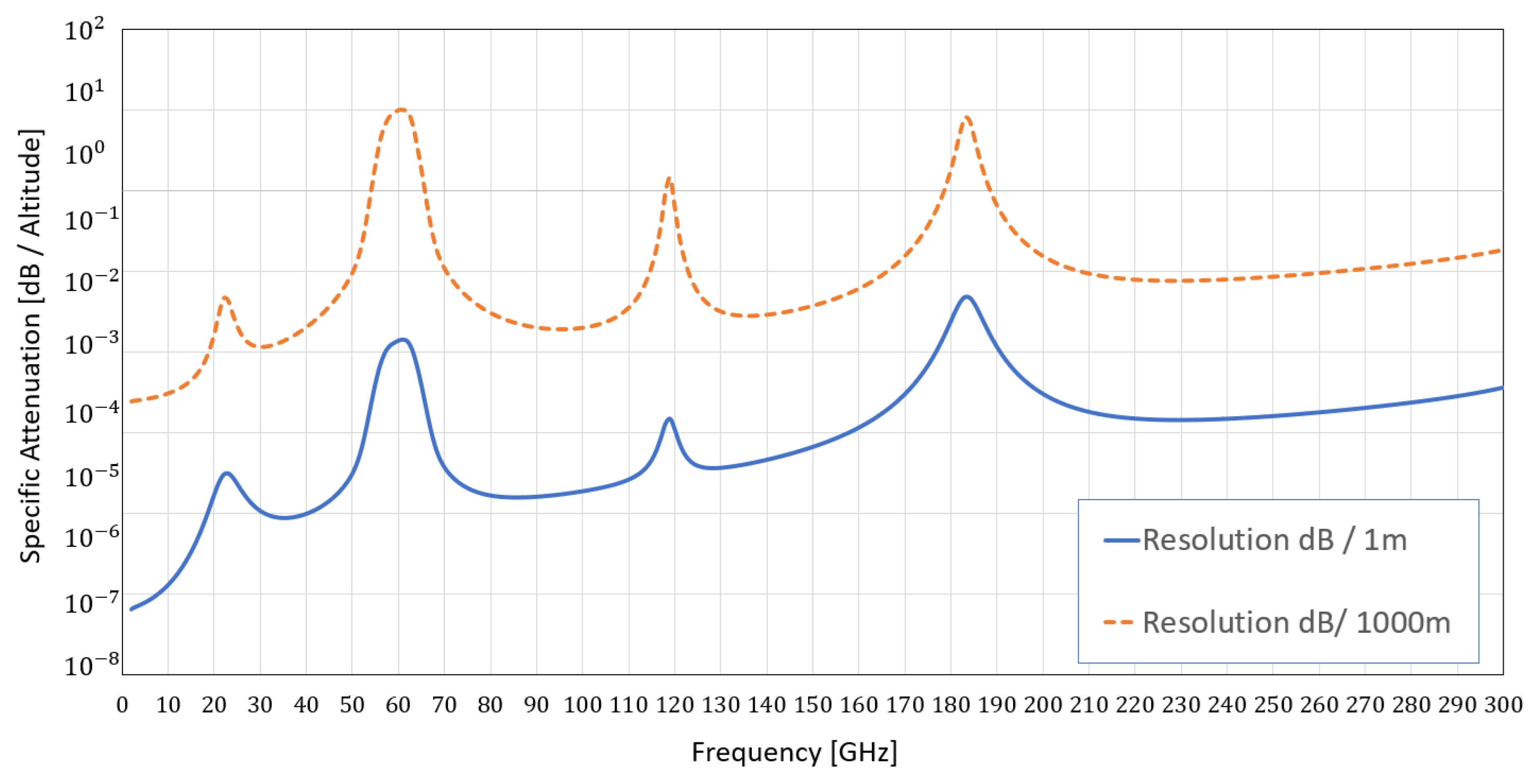
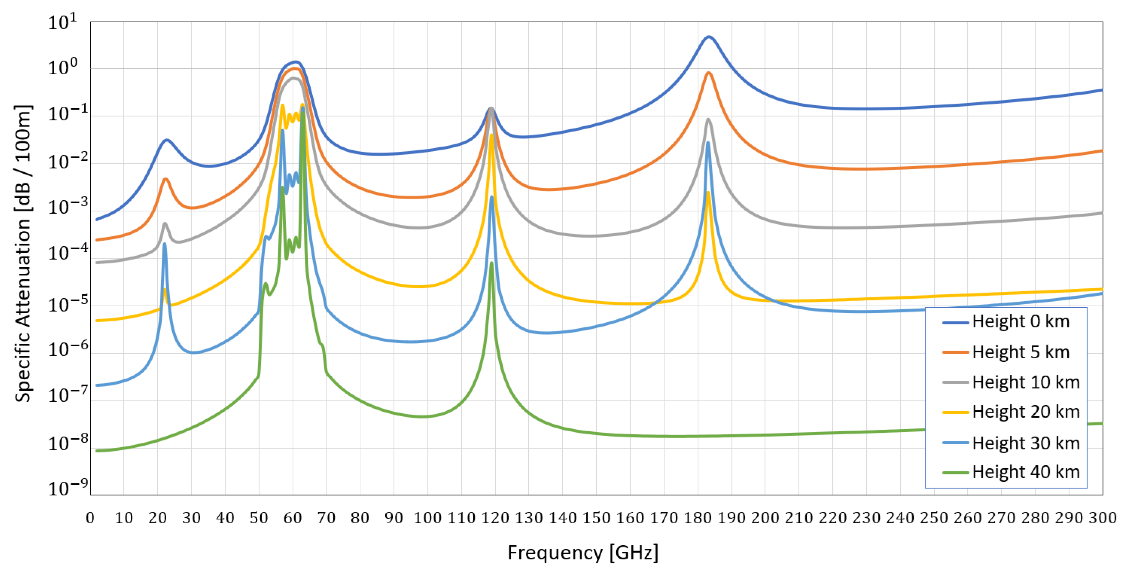
By combining all the fixed factors and all the free factors (atmospheric pressure, such as water vapor and temperature), we can get the signal’s atmospheric attenuation values in units of dB with good accuracy. The calculation of the atmospheric attenuation level was performed by the humidity model, which allows the calculation of the attenuation level with an accuracy of one meter at any desired frequency. Below are the graphical results of the attenuation at a height of one meter and km above the earth’s surface:

The analysis result shown in Figure 8 refers to the calculation on the Earth’s surface, with the main parameters being a temperature of 20 degrees, a water vapor level of 14 $g/m^3$, and an atmospheric pressure of 1017 hPa. As one increases in altitude, these values naturally decrease. Below is Figure 9 with the results of an analysis of inferiority at heights of 0, 5 km, 10 km, 20 km, 30 km, and 40 km. The accuracy of each measurement is 100 meters ( for example, if the height is 10 km, then the measured assumptions will be between 10.0 km and 10.1 km above the surface).

From the analysis of Figure 9, it is obtained that with the increase in frequency, there is an increase in the attenuation level in a logarithmically proportional way. At the frequencies 22 GHz and 184 GHz up to a height of 20 km above the earth, there is variation in the attenuation levels of the wave propagation. At the frequencies 63 and 113 GHz, there is attenuation at heights above 40 km above the ground. Variation in these values is a result of aerosols, physical effects, and the molecular compositions in the air.

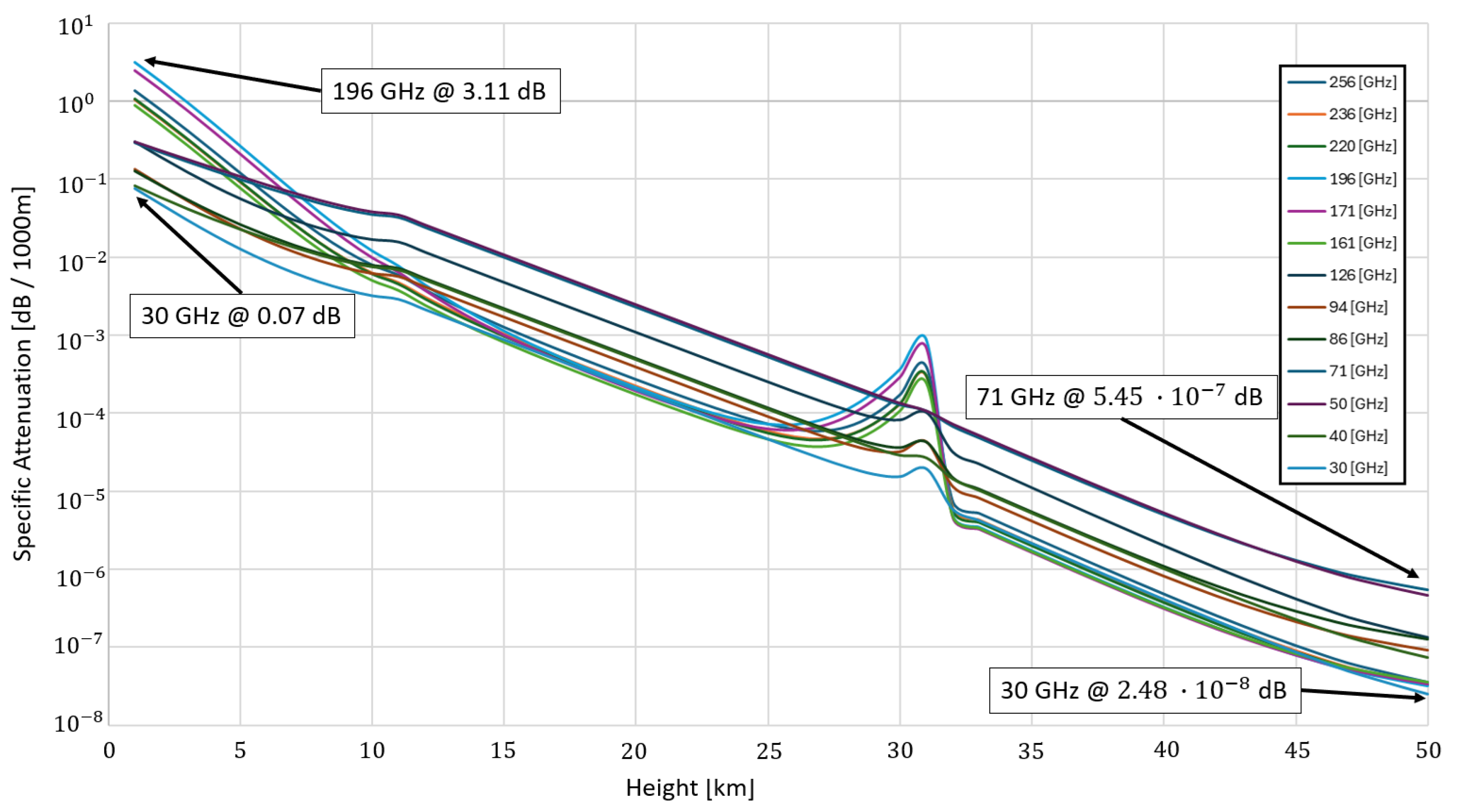
The FCC [50] document defines frequencies in which work is allowed in communication between the Earth and the satellite and between the satellite and the Earth. There is a division not only for these frequencies but also for geographical areas on Earth. The document’s purpose is to regulate transmission and reception frequencies so as not to create frequency and geographic overlap of frequencies. According to the document, there are specific frequencies in the EHF band. Prominent frequencies for use are 30 GHz,40 GHz,50 GHz,71 GHz,86 GHz,94 GHz,126 GHz,161 GHz,171 GHz,196 GHz,220 GHz,236 GHz, and 256 GHz. These frequencies received regulatory approval for satellite transmissions. Using the atmospheric attenuation modeling formulas 28, the attenuation values for each frequency can be calculated as a function of its height. Below are the results of the atmospheric attenuation values with a resolution of 1 km for frequencies intended for RF communication as a function of its height above the ground:

From the results of the analysis shown in Figure 10, it can be concluded that:

• The attenuation level in the clear sky in the EHF band at an altitude of up to 1 km in satellite communication frequencies ranges from 0.07 to 3.11 dB.
• At the height of 31 km, there are non-linear effects on the attenuation levels at different frequencies.
• At an altitude of 50 km, the attenuation level drops below ${10}^{-7}$ for the frequencies being tested.

By using the formula 27, cumulative attenuation values at different heights can be obtained. The formula makes it possible to give a cumulative attenuation value even in signal transitions not transmitted vertically from the Earth but at angles different than 90 degrees. The lower the elevation angle is than 90 degrees, the greater the total distance a signal goes through, and as a result, the attenuation will also increase. The formula 38 gives a calculation of the total distance that the signal goes through in its entire vertical height, preferably for different elevation angles with a resolution of one km.

$$\mathrm{L}\left[h\right]={\int }_0^h\left({\displaystyle \frac{1}{\sqrt{1-{\left(\frac{n_r\left(0\right)cos\left[\vartheta \left(0\right)\right]}{n_r\left(h^{\prime }\right)}\right)}^2}}}\right)d{h}^{\prime }$$

(38)

Table 3. Value of total distance that the signal goes through as a function of desired height and elevation angle.

Vertical height [km]	Elevation angle $\mathit{\vartheta }\left[{\mathit{n}}_0\right]$	Total distance[km]
1	901	1
1	80	1.01
1	60	1.15
1	40	1.55
1	30	2.92
1	10	5.75
25	901	25
25	80	25.38
25	60	28.86
25	40	38.88
25	30	73.04
25	10	143.54
100	901	100
100	80	101.54
100	60	115.46
100	40	155.56
100	30	292.32
100	10	575.43

¹ Signal transitions transmitted vertically from the earth.

Table 3. Value of total distance that the signal goes through as a function of desired height and elevation angle.

Vertical height [km]	Elevation angle $\mathit{\vartheta }\left[{\mathit{n}}_0\right]$	Total distance[km]
1	901	1
1	80	1.01
1	60	1.15
1	40	1.55
1	30	2.92
1	10	5.75
25	901	25
25	80	25.38
25	60	28.86
25	40	38.88
25	30	73.04
25	10	143.54
100	901	100
100	80	101.54
100	60	115.46
100	40	155.56
100	30	292.32
100	10	575.43

¹ Signal transitions transmitted vertically from the earth.

According to the cumulative attenuation function 27, the processes that affect the value are the initial angle $Q_0$ and the desired height perpendicular to the ground. In addition, two measurement modes should be separated: in the first mode, the earth is far from the sun, and the measurement is carried out in the shade (see formula 18) - Ex 0. 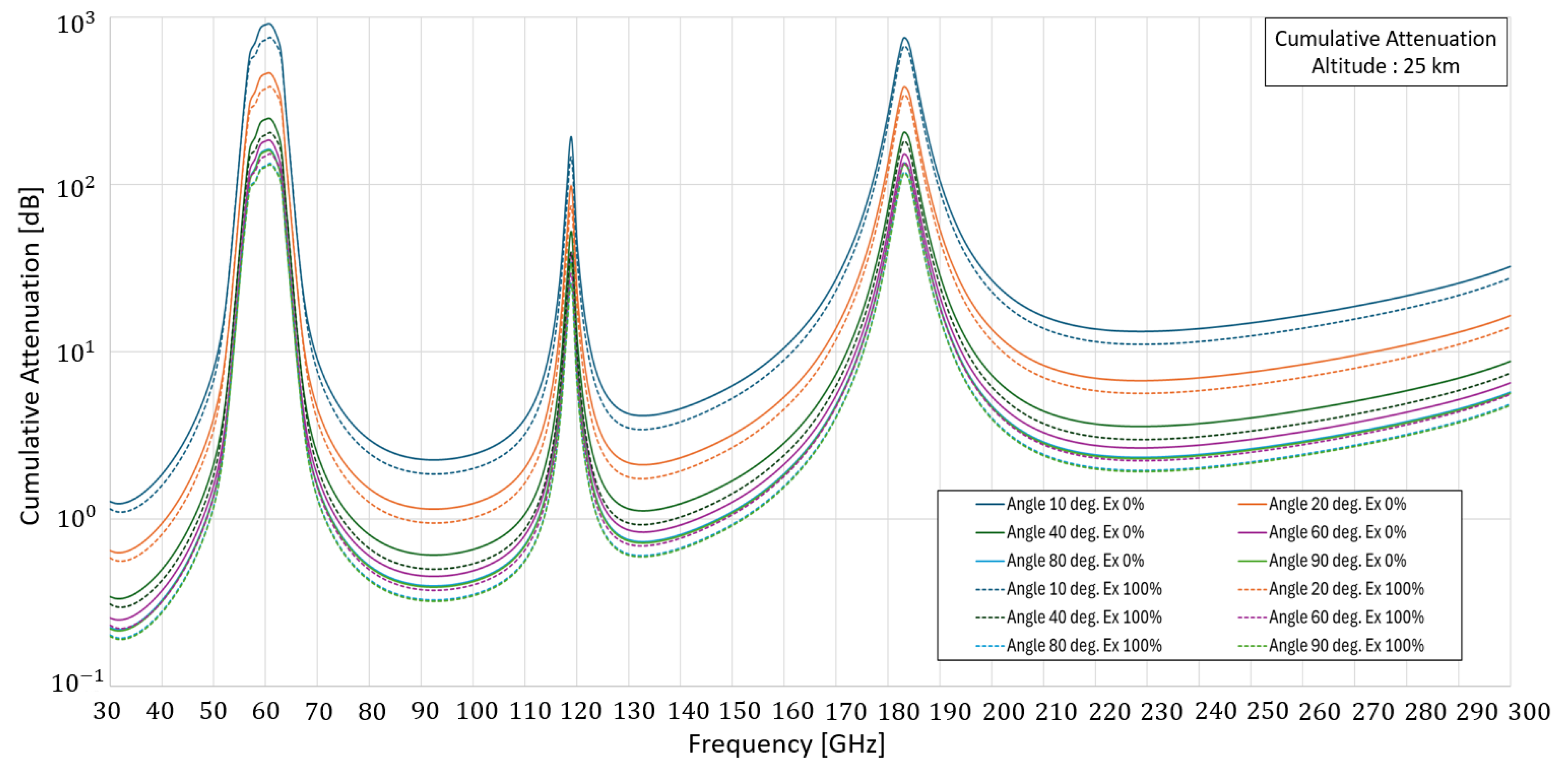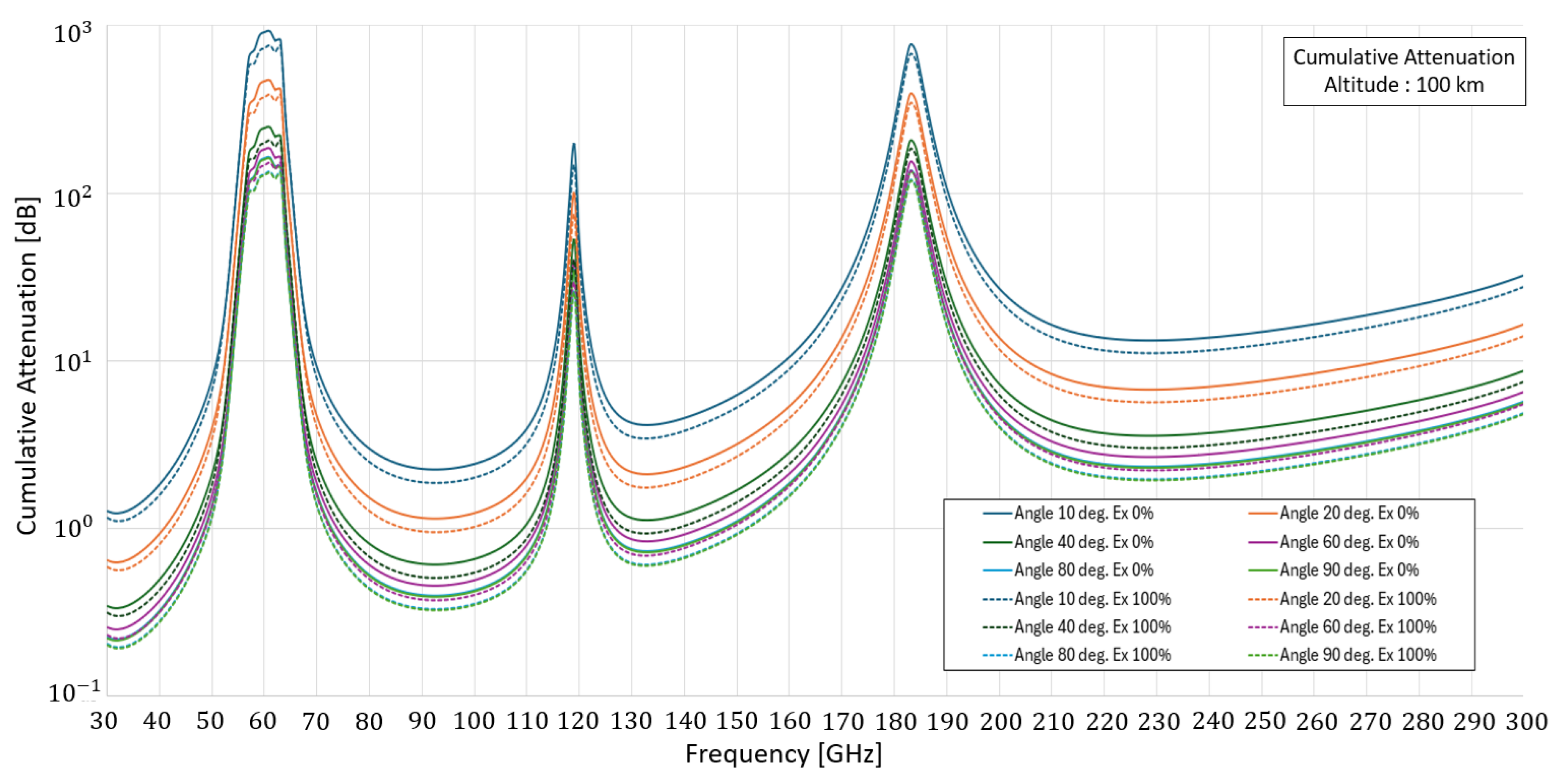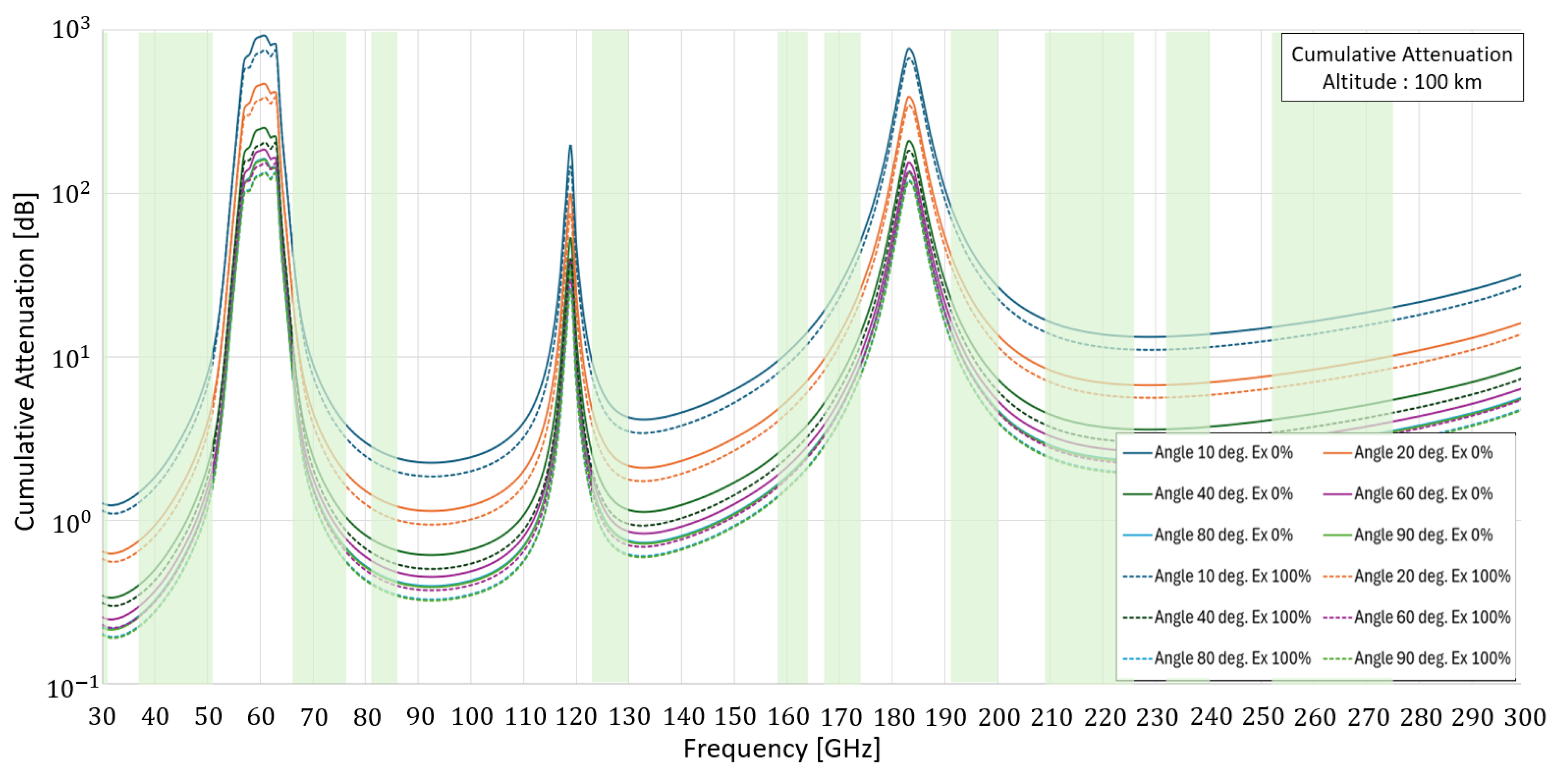Moreover, in the second mode, the earth is close to the sun, and the measurement is carried out using light (see formula 17) - Ex. 100. Each of the situations affects the final result. The following graphs will show analyses for heights perpendicular to the ground: 25 and 100 meters. The analyses were carried out in two modes: heat and cold.

5. Summary and Conclusions

In this article, an in-depth analysis was performed to calculate cumulative attenuation in the EHF frequency range in a clear sky at any height above the ground at different transmission angles. The goal was to present the entire analytical calculation process that allows reaching the value of cumulative attenuation. In the calculation, all the medium’s effects were considered. Based on the process, a similar calculation can be made for any height and desired transmission angle. The results show no linear relationship between the transmission angle and atmospheric humidity at the tested angle. It is a composition of functions that depend on many factors and affect the composition of the medium, such as gravity, atmospheric pressure, levels of water vapor and molecules in the air, etc. These factors affect not only the behavior of the assumptions at a specific frequency but also the refractive index at the same frequency in the same medium. This phenomenon leads to an alteration in the path of the electromagnetic wave, consequently causing a shift in the angle of refraction within the medium. At an angle perpendicular to the earth, the attenuation is the smallest, and as the transmission angle decreases, the attenuation level increases accordingly.

According to graphs 9 and 10, a different attenuation behavior affects the electromagnetic wave at different frequencies at each height above the earth. The conclusions presented refer only to the situation of a clear sky. At heights 30 km above the ground, there are strong attenuation effects in the 61 GHz, 119 GHz, and 183 GHz ranges. At the same height, in the 63 GHz and 184 GHz frequencies, the attenuation level is stronger than that at an altitude of 20 km. According to regulation, At operating frequencies in satellite communication, as shown in the FCC [50] table, up to a height of 1 km, attenuation at EHF frequencies ranges from 0.07 dB to 3.11 dB. At the same frequencies, at an altitude of 30 km, the maximum attenuation reaches up to ${10}^{-3}$ dB. At an altitude of 50 km, attenuation reaches $5·{10}^{-7}$ dB. As a result, as the altitude increases, the effect will be more negligible. For altitudes above 50 km, attenuation will not affect the electromagnetic wave.

According to graphs 11,12,13 and compared to the frequencies allowed to work in satellite communication according to the FCC tables, the value of the cumulative attenuation is higher in a state of darkness and far from the sun than the state when the sun is close to the earth, and there is light. Below is a table summarizing all the analyses of cumulative attenuation in a clear sky:

According to the values shown in Table 4,Table 5,Table 6, and Table 7, there is no significant difference between cumulative attenuation in a clear sky at an altitude of 25 km and an altitude of 100 km. The main effects are transmission angle above the ground, frequency, transmission time, and season. The lowest values can be seen in Table 5. Graph 10 shows that for heights above 100 km, cumulative attenuation in a clear sky will not change much for satellite transmission and reception frequencies; additional cumulative attenuation will be lower than 0.01 dB (Up-Link & Down-Link). For GEO satellites where the transmission and reception angle varies between 90 and 40 degrees, the maximum cumulative attenuation that can be obtained will be 10.7 dB. LEO satellite angles can reach up to 10 degrees relative to the ground. In these cases, the frequency is fundamental. Up to frequencies of 126 GHz, cumulative attenuation ranges up to 8 dB; above this frequency, they can also reach 39.5 dB. Effective communication systems in modern society rely heavily on transmitting electromagnetic waves. However, atmospheric conditions, including weather conditions, atmospheric pressure, and humidity, can significantly affect the transmission of these waves from the attenuation they or their effects create. The attenuation level varies depending on the frequency of the electromagnetic wave, the angle of transmission, and the weather conditions. Understanding the effects of atmospheric conditions on the transmission of electromagnetic waves is essential to developing reliable and efficient communication systems. The mathematical analysis presented in this document emphasizes that there is no linear relationship between cumulative atmospheric attenuation and frequency. The relationship is created from the composition of functions that depend on several factors that affect the composition of the medium through which the electromagnetic wave passes. As the angle increases, the transmission medium of an electromagnetic wave will increase, resulting in a cumulative attenuation increase. Also, the shorter the wavelength, the greater the attenuation, although this is not always the case. There are cases where there is an effect of resonance and vibration frequencies of molecules in which the attenuation is higher. In addition to attenuation varying between cold and warm temperatures, total attenuation is expected to be higher at cold temperatures. The analysis results showed that the ratio of the attenuation effect in the transition from 25 km to 100 km can cause additional attenuation varying between 0.02 dB and 6 dB on average at frequencies that have regulation for the transmission and reception of a satellite communication signal up to a frequency of 300 GHz.