Submitted:
15 November 2024
Posted:
18 November 2024
Read the latest preprint version here
Abstract
This paper presents a revival of FORTRAN 66 code which calculates flow through curved pipes. Results from the code were originally presented in [Greenspan, D. Secondary flow in a curved tube. J. Fluid Mech. 1973, 57, 167-176]. We demonstrate a step-by-step code revival process and compare original (coarse) results to updated (fine) solutions. The purpose of our paper is to make the code available as modern Fortran for the scientific community. The code runs quickly on modern hardware architectures and enables fast understanding of the physical effects included.
Keywords:
fluid motion in a curved pipe
; laminar flow
; code revival
; FORTRAN 66
; modern Fortran
1. Introduction
The theoretical treatment of laminar flow in curved pipes was pioneered by Dean in the late 1920s [1,2]. He showed that in addition to a displacement of streamwise flow, a secondary flow also exists, taking the form of two vortices, the so-called Dean vortices. A constant D, the Dean number, was identified as the key parameter:
where is the bulk Reynolds number, a is the pipe radius and L is the radius of curvature of the curved pipe. Dean [1] obtained simplified equations of motion for the approximation , which can be interpreted as [2].
Dean [1] obtained theoretical solutions to the equations for the range and following this, McConalogue and Srivastava expanded the solutions numerically to [3]. In this paper we treat a subsequent study by Greenspan and Schubert [4,5], where numerical solutions were extended to . This extension was done with a FORTRAN 66 code which is available as an Appendix in [4]. The purpose of our paper is to convert - and thus revive - this code to modern Fortran. The reason for this is twofold: (i) we need the revived code for planned future research and (ii) we want to make this code available to the scientific community for others who may need a fast and efficient code to calculate basic solutions of laminar flow in slightly curved pipes.
On a personal note, I have previous experience writing and running FORTRAN 77 code on an IBM mainframe at JET [6] during the period 1997-1998. Thus, the task at hand, to convert FORTRAN 66 code, was feasible.
2. Code Revival
There were three aspects to the code revival, and they are treated in the three subsections below:
- Digitise the scanned document
- Convert the FORTRAN 66 code to modern Fortran
- Debugging and testing of the code
2.1. Digitisation
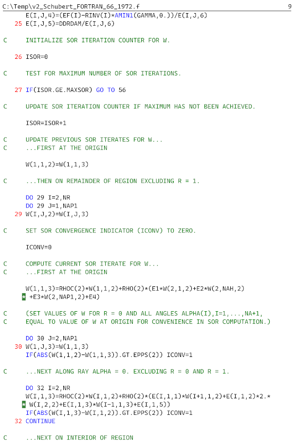
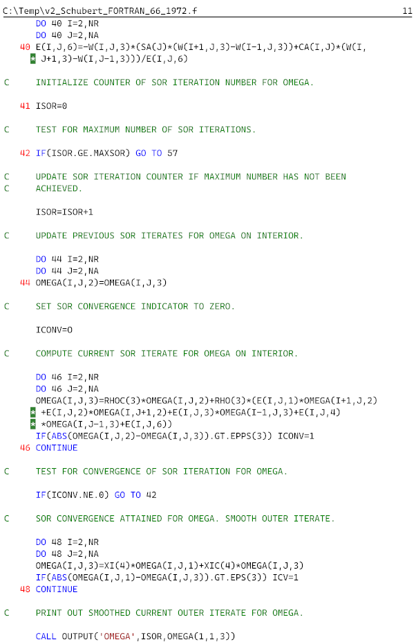
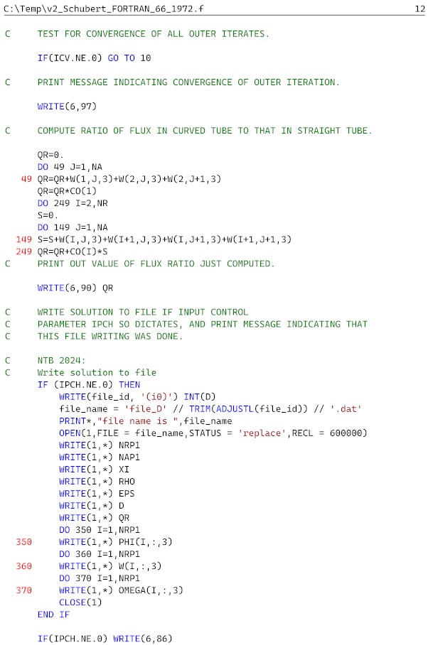
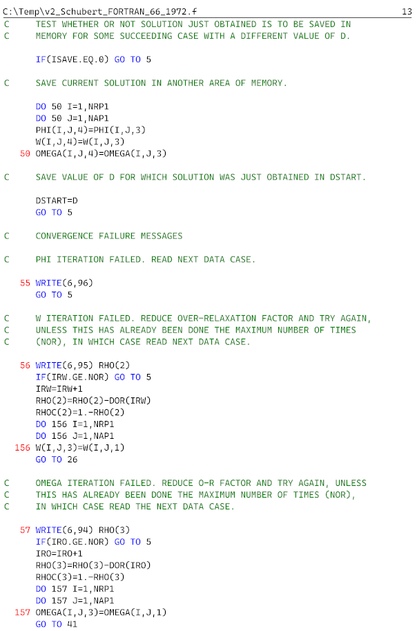
We note that the original FORTRAN 66 code is only available in [4] and not available in the official journal paper [5]. As can be seen, the scanned document [4] has a quite poor quality, making in challenging to perform the optical character recognition (OCR) needed. However, with 12 pages (∼600 lines) of code, it would be very cumbersome to retype the code entirely by hand
We did not attempt to improve the quality of the scanned document before conversion.
Our initial attempts at extracting characters from the scanned document was done using Python with EasyOCR [7] and PyTesseract [8]. However, these tools performed poorly on the document.
Our next attempt was with two online converters [9,10]. The results were better than for the Python tools, but still with a correct percentage of around 50%.
The best conversion, with a success rate of roughly 80%, was the Amazon Textract tool from Amazon Web Services (AWS) [11].
In the end, we used the AWS tool to generate the initial digital file and combined it with the output from the two online converters. And finally, a human correction was needed for around 10% of the code.
2.2. Conversion
2.3. Debugging and testing
At this stage we had a complete code available, the final step being to debug and test the code.
We chose to use a laptop with Microsoft Windows 11 [14] installed. Microsoft Visual Studio [15] was installed as the graphical user interface along with the Intel Fortran Compiler (ifx) [16]. In terms of Fortran versions, ifx uses the latest standards from Fortran 2018 and some Fortran 2023 features. In that sense, we consider the updated code to represent modern Fortran.
What remained was to compile (build solution) and systematically resolve the errors. Some sections were updated, for example replacing the reading of and writing on punch cards with files. Another major change was to make an IF statement to loop over all D values analysed in [4,5].
The final result of the steps is the modern Fortran code provided in Appendix A.
3. Results
All post processing in this section was done using GNU Octave [17].
3.1. Comparison to Original Findings
We include two figures with contour plots of and w, Figure 1 and Figure 2, to facilitate a direct comparison to Figure 3 and 4 in [5]. Here, is the non-dimensional stream function for the secondary flow and w is the non-dimensional velocity in the streamwise direction. Only the upper half of the pipe is calculated by the Fortran code, we mirror this to the lower half for clarity of exposition. 0 (180) degrees indicate the outboard (inboard) positions, respectively.
The results match the original results very well, both in position and magnitude. Again, the curves move clockwise up to and then counter-clockwise for larger D. And a certain waviness is observed for the core w curves for , which was speculated to perhaps indicate a beginning transition to turbulence [5].
3.2. Improvements
Having a complete modern Fortran code available enables improvements to e.g. the computational grid resolution. The original resolution was and . In the code in Appendix A, these resolutions are named NR and NA, respectively. We updated the code to run with double resolution, both for r and . To distinguish the grid resolutions, we call them "original" and "updated".
We compare original and updated contour plots for and w in Figure 3 and Figure 4. The two largest values of D are compared; qualitatively, the results are very similar, although the contours of the updated resolution are more smooth than those of the original resolution.
A topic of interest for our future research is how the peak w value () moves as a function of D. This is shown in Figure 5, where both the position and magnitude of are included. The values are compared for the original and updated resolution; we observe that there is a substantial difference in the maximum position, but not in the maximum value of w. For reference, values from [3] are included, which agree with the present values for smaller values of D, but deviate for larger D.
An important effect of the secondary flow is the blockage effect, i.e. that it obstructs the streamwise flow. This is also calculated in the Fortran code and shown in Figure 6. Here, the flux (or flow rate) is normalised to that of a straight pipe.
4. Discussion
It has been discussed whether flow in curved pipes only depends on the Dean number, or if one should separate studies into separate and curvature effects. Now it is indeed clear that such a separation is important for turbulence studies, see e.g. [18]. For the case we treat with slightly curved pipes, the transition to turbulence is subcritical, which is the same as for straight pipes.
From experimental investigations with higher curvature [19], it is interesting to note the persistence of structures in turbulent flow similar to those identified in laminar flow. Perhaps the laminar flow structures form a skeleton/seed which turbulence builds on?
5. Conclusions
In this paper, we have presented a case study on how to revive older code (FORTRAN 66) to modern Fortran. This code revival has enabled fast calculations of laminar flow through slightly curved pipes. The basis was [5], with the original code being provided in [4]. We hope that our work serves as a template and inspiration for other scientists who have a need for bringing older code back to life again. Also, the modern Fortran code in Appendix A is now available to the scientific community as a fast method to obtain a physical picture of streamwise and secondary flow in curved pipes.
After the code was operational, we tested increasing the grid resolution and found that the position of the maximum streamwise velocity as a function of D was sensitive to this change.
The code can be modified in other ways to e.g. extract information on the stream function for the secondary flow or to make a more detailed study using smaller steps in D.
We plan to use the code in the future to facilitate interdisciplinary work on fluids and plasmas which was initiated in [20].
Funding
This research received no external funding.
Data Availability Statement
The data presented in this paper can be generated by using the modernised Fortran code in Appendix A.
Conflicts of Interest
The author declares no conflict of interest.
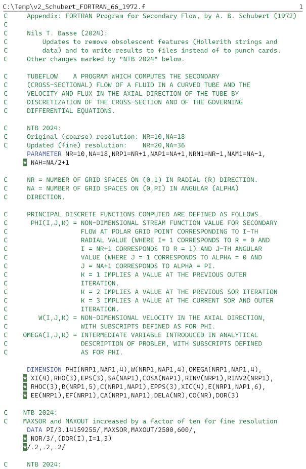
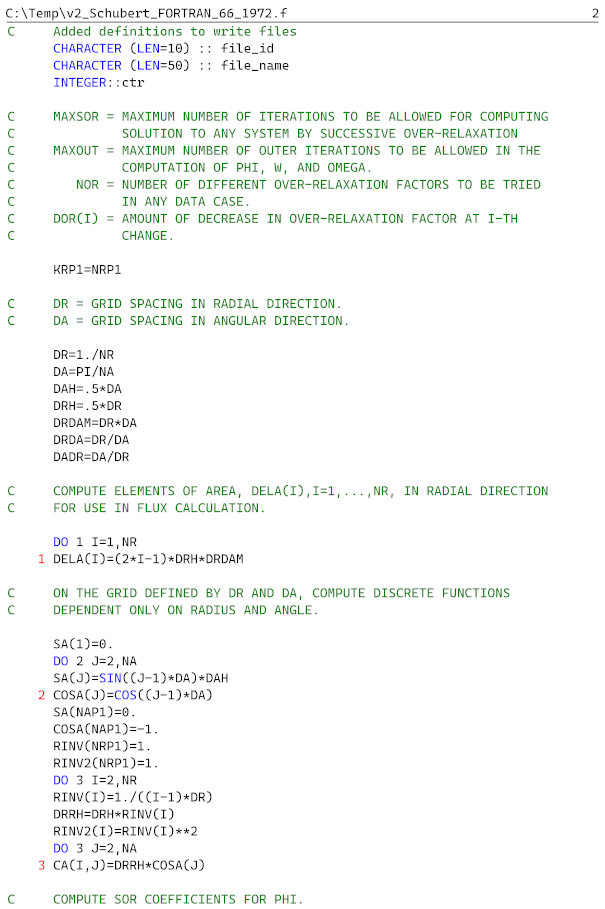
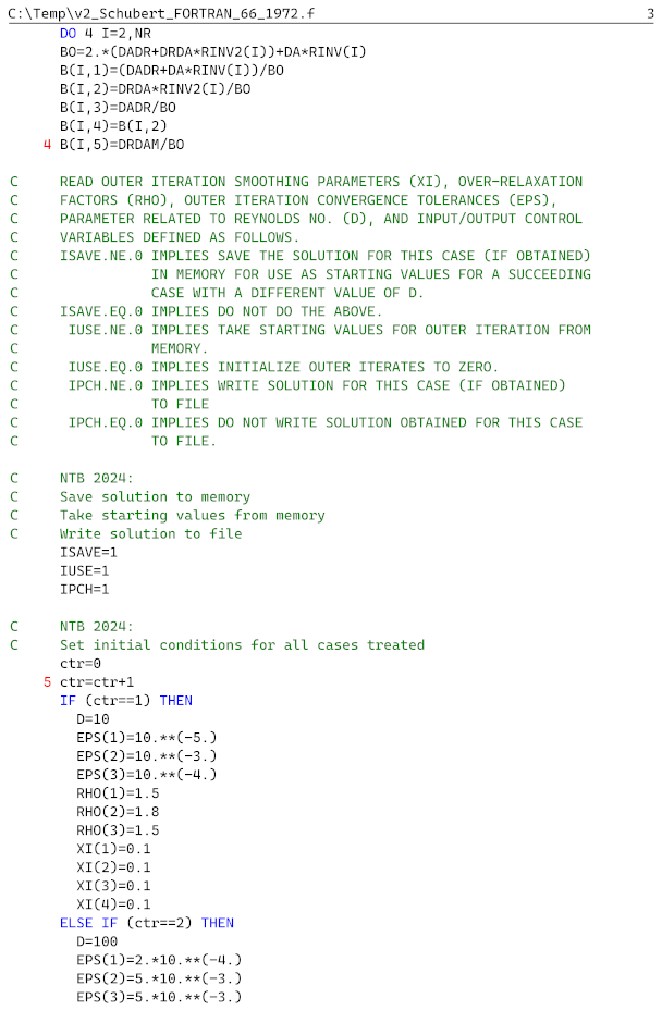
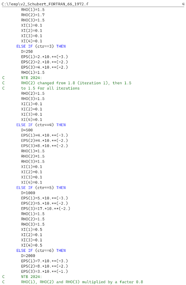
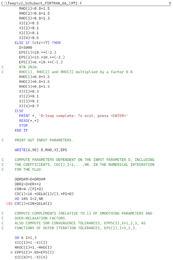
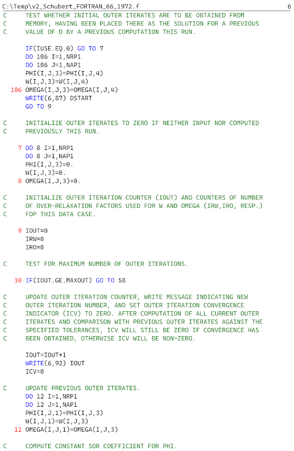
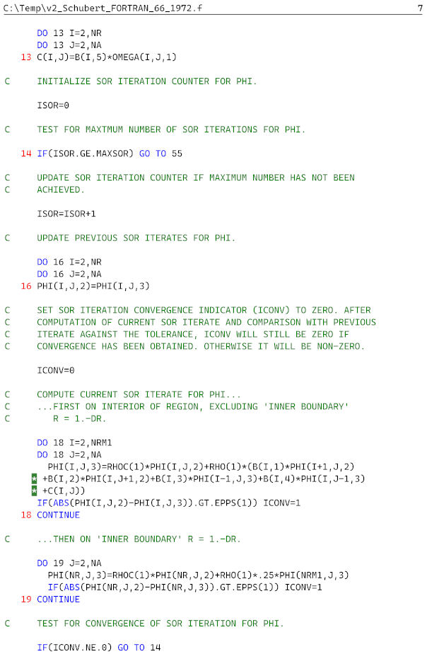
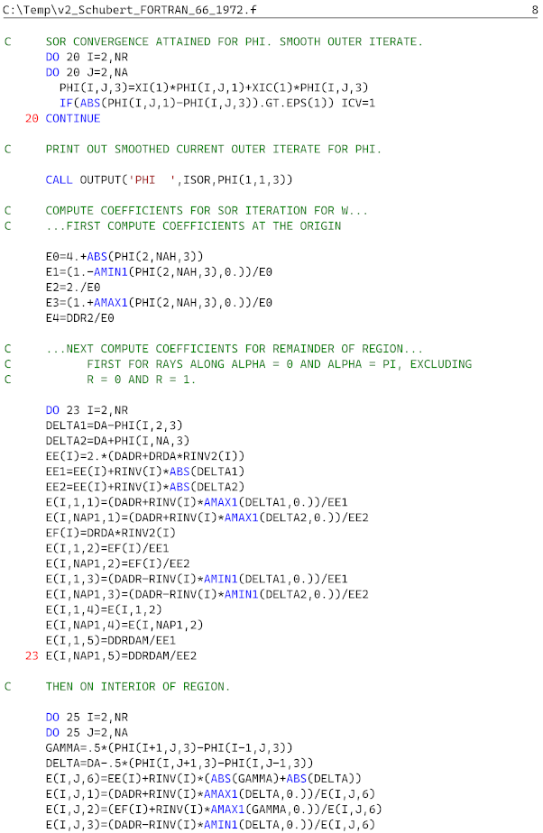
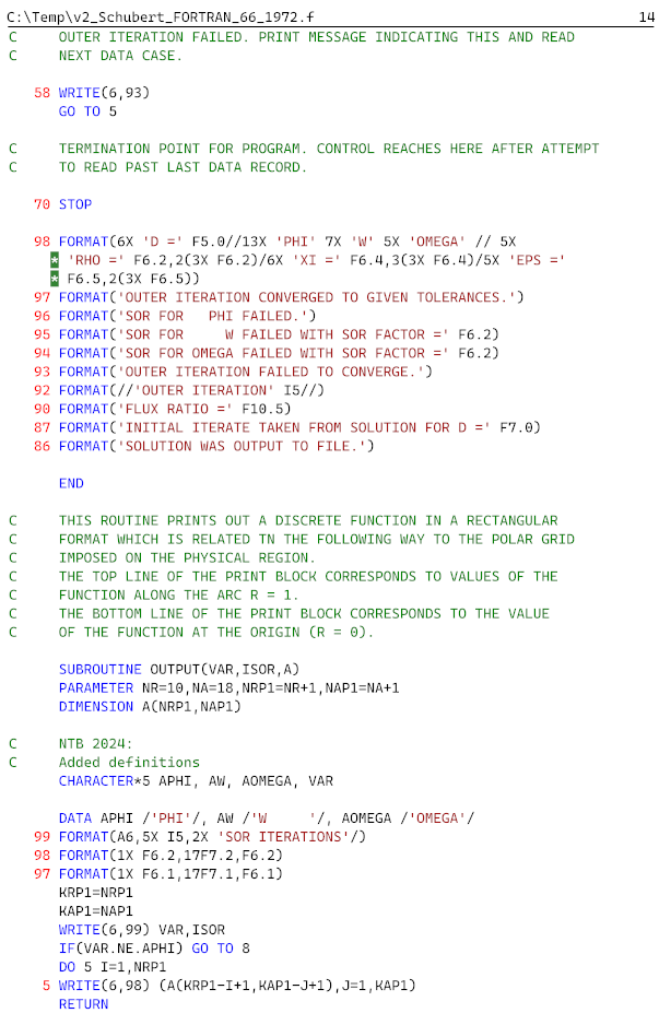
Appendix A Modernised Fortran Code
This appendix includes the modernised Fortran version of the original FORTRAN 66 code written by A.B.Schubert in 1972 [4].
Compiling and running the solution creates a separate file for each value of D.

References
- Dean, W.R. Note on the motion of fluid in a curved pipe. Phil. Mag. 1927, 4, 208–223. [Google Scholar] [CrossRef]
- Dean, W.R. The stream-line motion of fluid in a curved pipe. Phil. Mag. 1928, 5, 673–695. [Google Scholar] [CrossRef]
- McConalogue, D.J.; Srivastava, R.S. Motion of fluid in a curved tube. Proc. Roy. Soc. A. 1968, 307, 37–53. [Google Scholar] [CrossRef]
- Greenspan, D; Schubert, A.B. Secondary flow in a curved tube. University of Wisconsin, Computer Sciences Department, Technical Report #155 1972. Available online: https://minds.wisconsin.edu/handle/1793/57756.
- Greenspan, D. Secondary flow in a curved tube. J. Fluid Mech. 1973, 57, 167–176. [Google Scholar] [CrossRef]
- Krom, J.G. The evolution of control and data acquisition at JET. Fus. Eng. Des. 1999, 43, 265–273. [Google Scholar] [CrossRef]
- EasyOCR. Available online: https://pypi.org/project/easyocr/.
- PyTesseract. Available online: https://pypi.org/project/pytesseract/.
- PDF.ai. Available online: https://pdf.ai/tools/ocr-pdf.
- MaxAI.me. Available online: https://www.maxai.me/pdf-tools/pdf-ocr/.
- Amazon Web Services. Available online:; https://aws.amazon.com/.
- Metcalf, M.; Reid, J. Fortran 90/95 Explained; Oxford University Press: Oxford, UK, 1996. [Google Scholar]
- OpenAI. Available online: https://chatgpt.com/.
- Microsoft Windows 11 Enterprise. Available online: https://www.microsoft.com/en-us/microsoft-365/windows/windows-11-enterprise.
- Microsft Visual Studio 2022. Available online: https://visualstudio.microsoft.com/downloads/.
- Intel oneAPI HPC Toolkit 2024.2. Available online: https://www.intel.com/content/www/us/en/developer/tools/oneapi/hpc-toolkit.html#gs.i3q2al.
- GNU Octave, version 9.2.0. Available online: https://octave.org/.
- Canton, J.; Rinaldi, E.; Örlü, R.; Schlatter, P. Critical point for bifurcation cascades and featureless turbulence. Phys. Rev. Lett. 2020, 124, 014501. [Google Scholar] [CrossRef] [PubMed]
- Kühnen, J.; Holzner, M.; Hof, B.; Kuhlmann, H.C. Experimental investigation of transitional flow in a toroidal pipe. J. Fluid Mech. 2014, 738, 463–491. [Google Scholar] [CrossRef]
- Basse, N.T. The chimera revisited: Wall- and magnetically-bounded turbulent flows. Fluids 2024, 9, 34. [Google Scholar] [CrossRef]
Figure 1.
Original contour plots for , , , and .
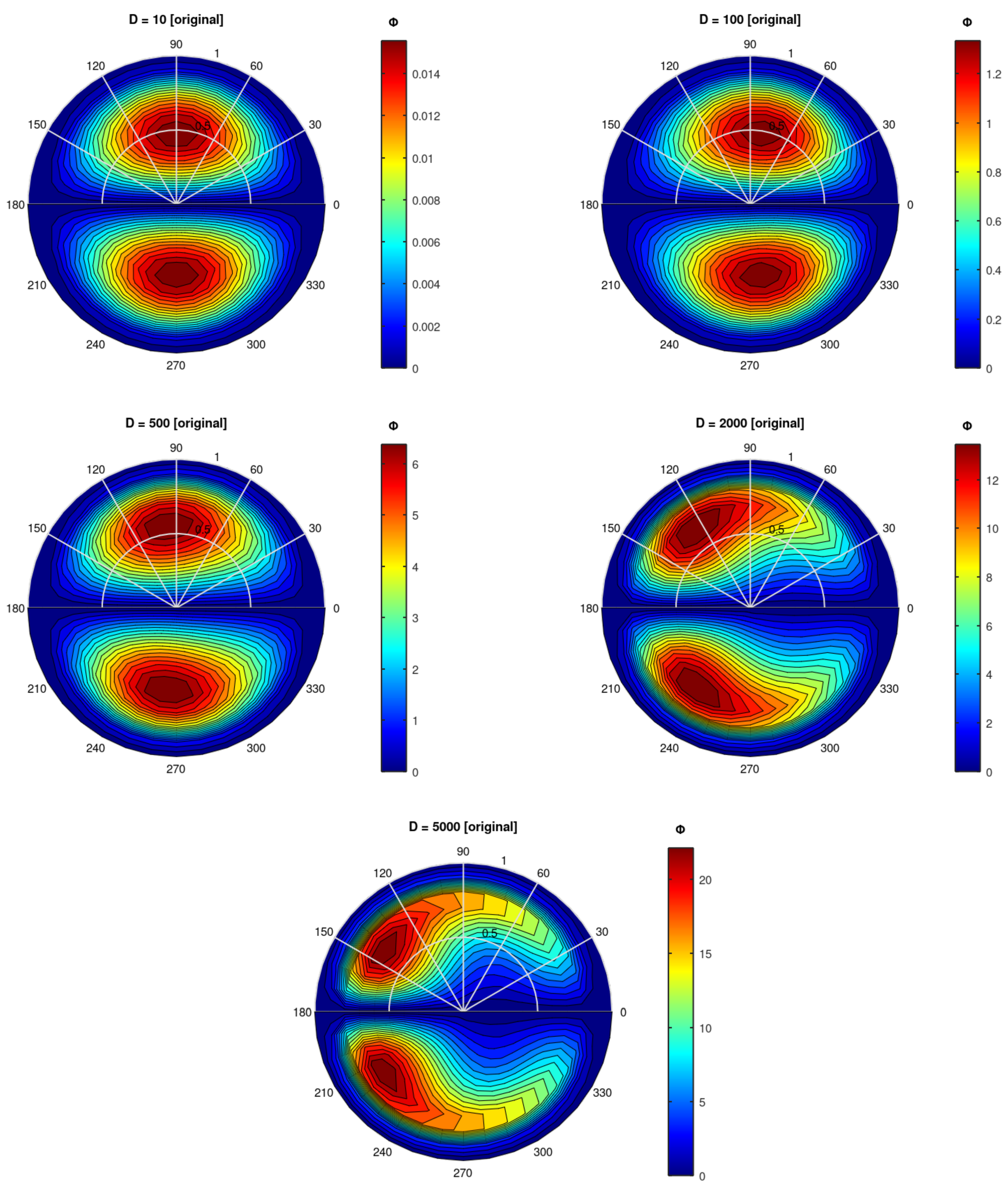
Figure 2.
Original w contour plots for , , , and .
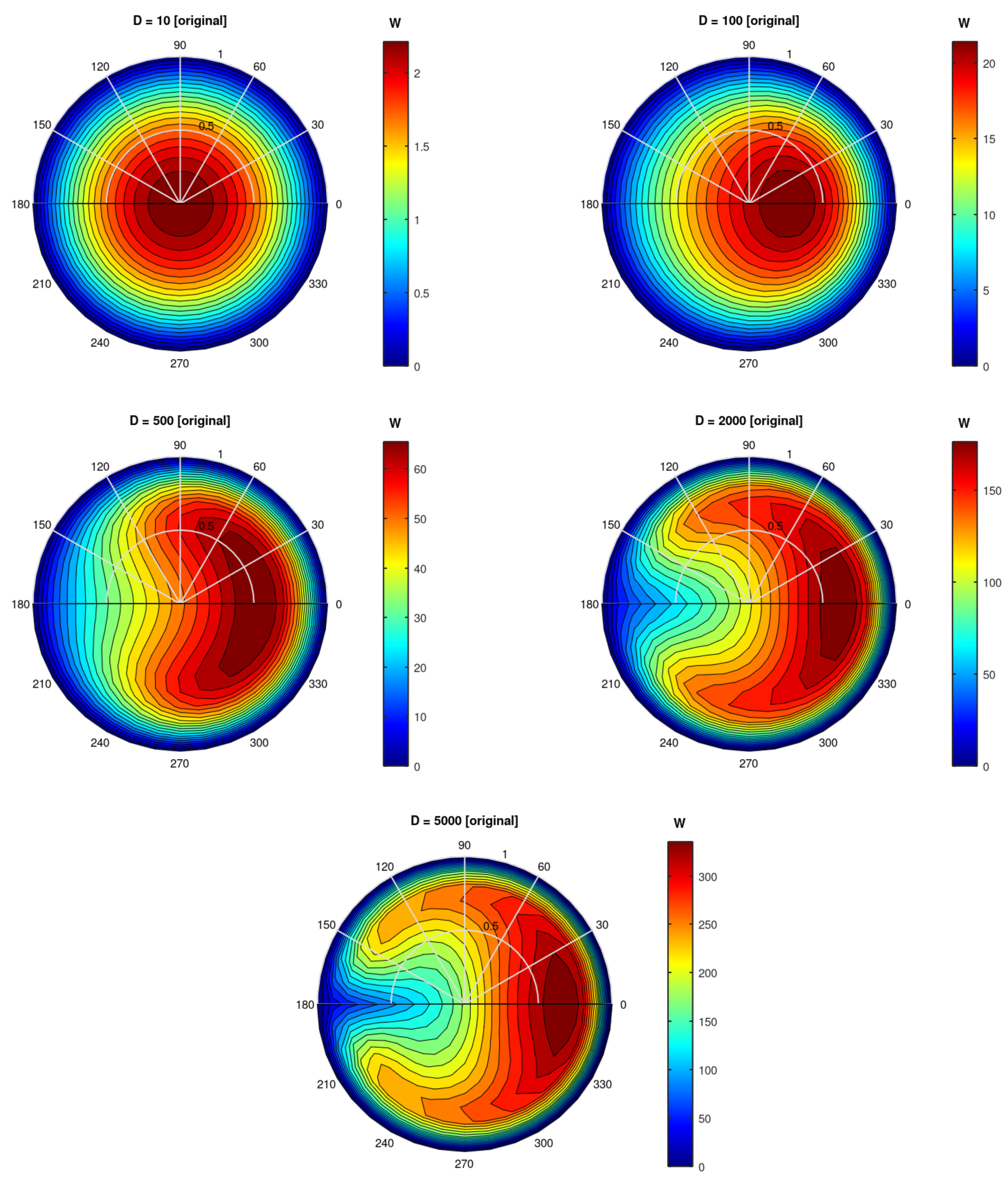
Figure 3.
contour plots for and . Left-hand column: Original (coarse) resolution, right-hand column: Updated (fine) resolution.
Figure 3.
contour plots for and . Left-hand column: Original (coarse) resolution, right-hand column: Updated (fine) resolution.
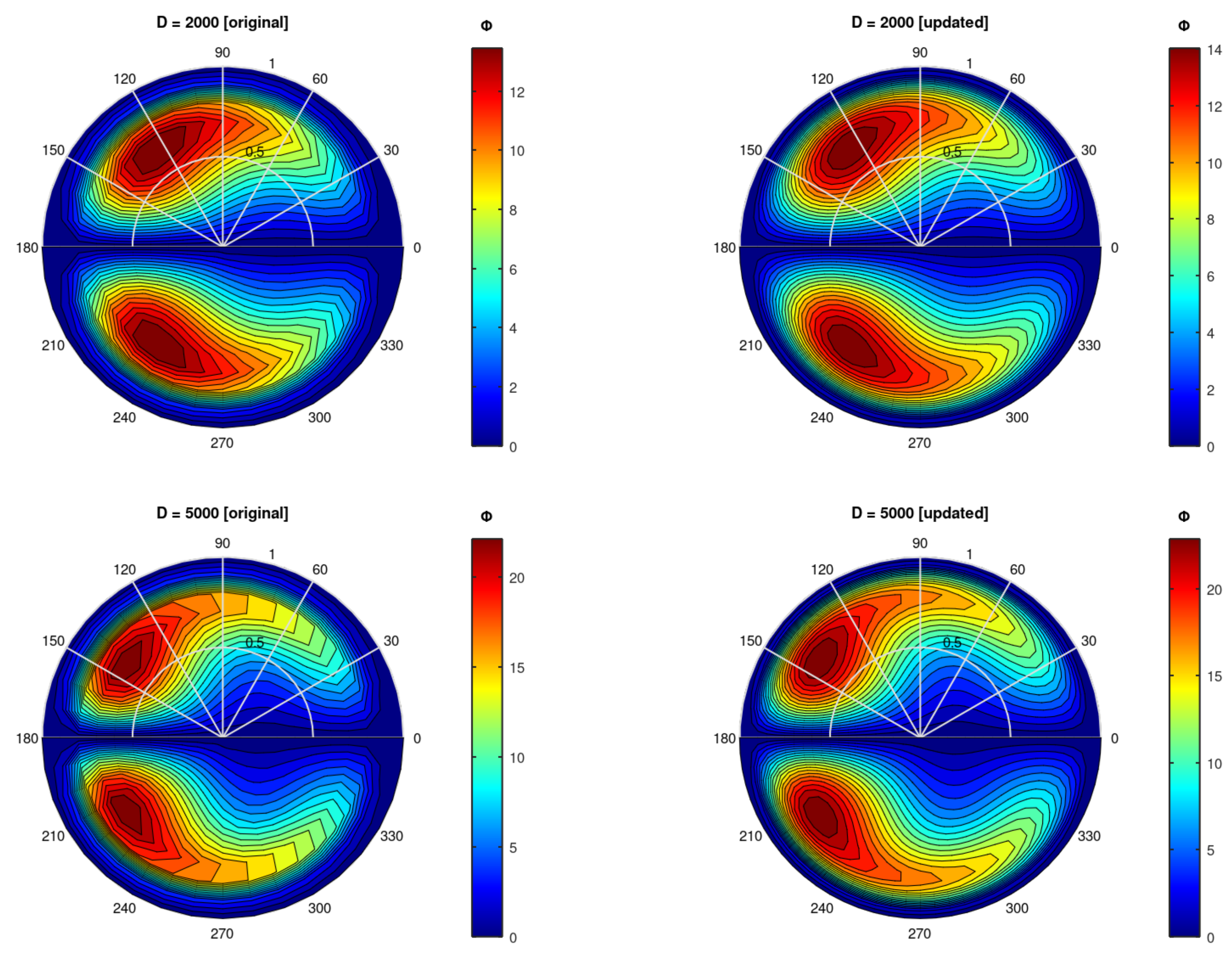
Figure 4.
w contour plots for and . Left-hand column: Original (coarse) resolution, right-hand column: Updated (fine) resolution.
Figure 4.
w contour plots for and . Left-hand column: Original (coarse) resolution, right-hand column: Updated (fine) resolution.
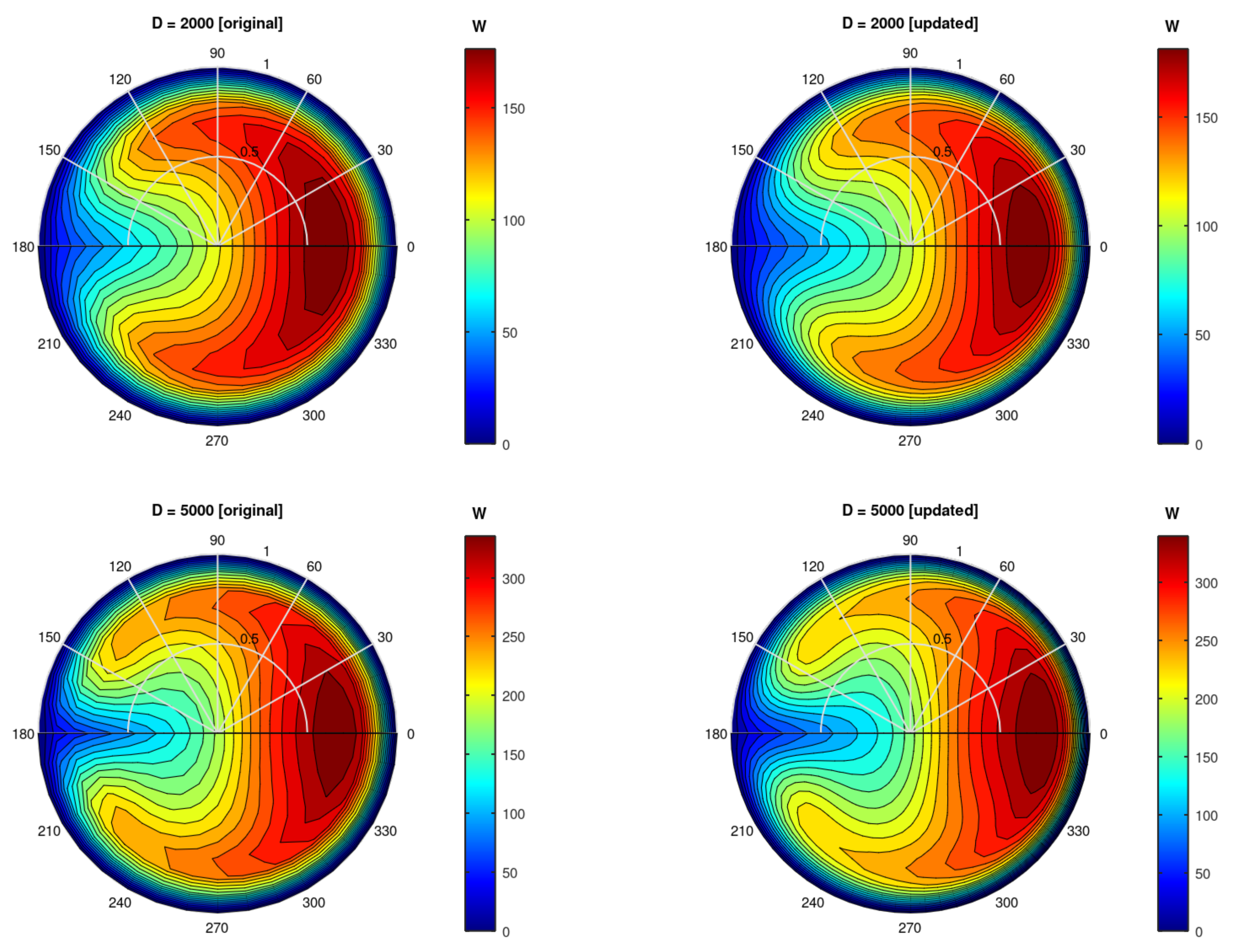
Figure 5.
Left-hand plot: Normalised radius for maximum streamwise velocity as a function of D, right-hand plot: Value of as a function of D.
Figure 5.
Left-hand plot: Normalised radius for maximum streamwise velocity as a function of D, right-hand plot: Value of as a function of D.
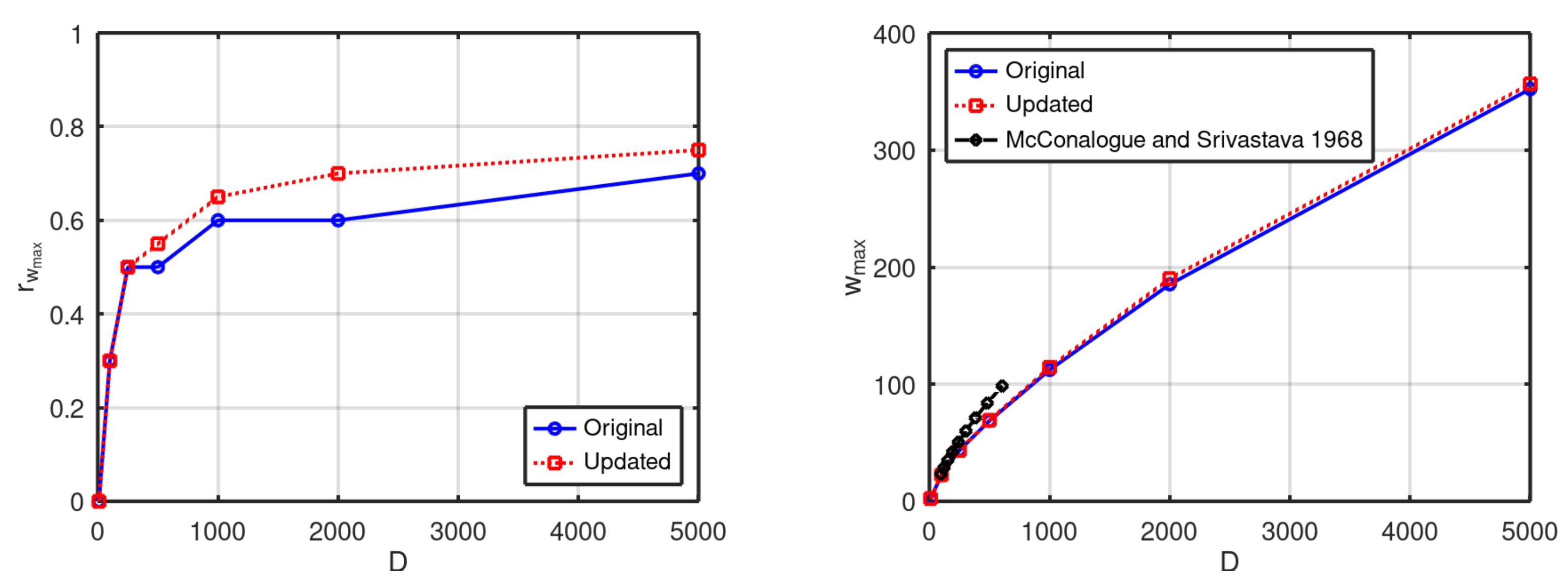
Figure 6.
Streamwise flux as a function of D.

Disclaimer/Publisher’s Note: The statements, opinions and data contained in all publications are solely those of the individual author(s) and contributor(s) and not of MDPI and/or the editor(s). MDPI and/or the editor(s) disclaim responsibility for any injury to people or property resulting from any ideas, methods, instructions or products referred to in the content. |
© 2024 by the authors. Licensee MDPI, Basel, Switzerland. This article is an open access article distributed under the terms and conditions of the Creative Commons Attribution (CC BY) license (http://creativecommons.org/licenses/by/4.0/).
Copyright: This open access article is published under a Creative Commons CC BY 4.0 license, which permit the free download, distribution, and reuse, provided that the author and preprint are cited in any reuse.


