Submitted:
09 November 2024
Posted:
12 November 2024
You are already at the latest version
Abstract
Over the past few years, there has been significant research on the Internet of Things (IOT), with a major challenge being network security and penetration. Security solutions require careful planning and vigilance to safeguard system security and privacy. Adjusting the weights of neural networks has been shown to improve detection accuracy to some extent. In attack detection, the primary goal is to enhance the precision of attack detection using machine learning techniques. The paper details a fresh approach for adjusting weights in the random neural network to recognize attacks. Reviews of the method under consideration indicate better performance than random neural network methods, Nearest Neighbor, and Support Vector Machine (SVM). Up to 99.49% accuracy has been achieved in attack detection, while the random neural network method has improved to 99.01%. The amalgamation of the most effective approaches in these experiments through a multi-learning model led to an accuracy improvement to 99.56%. The proposed model required less training time compared to the random neural network method.
Keywords:
IOT
; Machine Learning
; Cyber Security
; Metaheuristic Algorithms
; Random Neural Network
; Evolutionary Intelligence
1. Introduction
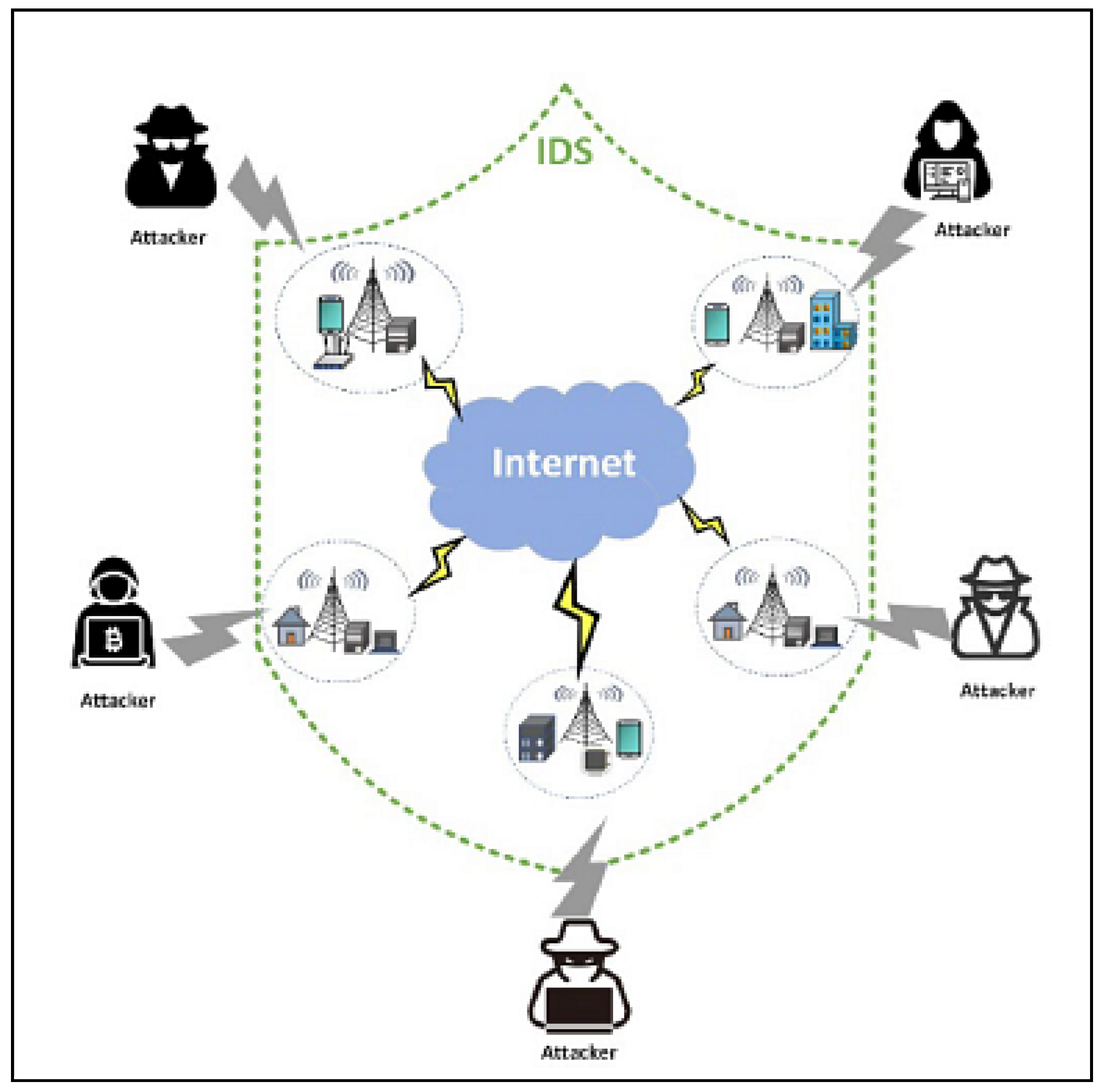
The Internet of Things (IOT) is a network composed of devices equipped with special sensors for detecting monitoring areas and transmitting collected data to end users. The IOT is widely used in many scenarios, such as COVID-19, healthcare, environmental monitoring, smart buildings, and more. The global IOT market was reported by Gartner to be nearly 6 billion devices in 2020. McKinsey estimates that by 2025, IOT will be worth around 11 trillion dollars. Additionally, the rise of 6G wireless communications and mobile edge computing can support the expansion of IOT devices [1]. IOT networks are highly heterogeneous networks, where various types of nodes and connections multiply rapidly. The IOT framework encompasses virtual and physical environments, as well as other developing technologies. IOT environments often consist of four main entities including devices, various IOT users, edge gateways, and cloud storage servers [2]. The merging of sensors and wireless communication has facilitated the expansion of the Internet of Things. Wireless sensor nodes play an essential role in the structure of IOT networks [3]. IOT differs from Wireless Sensor Network (WSN) in that IOT devices are connected to the Internet, whereas WSN is not directly connected. Within these networks, sensors link to a central node referred to as a cluster head, which is then connected to the Internet [4]. The scope of IOT goes beyond smart homes and internet-connected household devices. Cities are also included in this technology and utilized in various industries to monitor products with interconnected sensors. The Internet of Things (IOT) is highly diverse due to the separate evolution of its devices and networks, with limited energy and hardware resources. Moreover, IOT networks have witnessed the growth and standardization of a broad array of protocols to support IOT applications, which encompass wireless communication technologies like (ZIGBEE, BLE, LORAWAN, SIGFOX) [5]. Enhancing network efficiency and defending against attacks are crucial challenges in IOT networks. The efficiency of the entire system can be compromised as these attacks have the ability to damage or weaken the transmitted packets [39]. To achieve complete security in the IOT network in today's world, in addition to attack prevention equipment, systems called Intrusion Detection Systems (IDS) are required to detect intrusions if an intruder bypasses security equipment and enters the network, recognize it, and think of a solution to deal with it, addressing these issues requires very scalable solutions [6]. An Intrusion Detection System is a cybersecurity approach that watches and analyzes network traffic to prevent and identify potential malicious attacks. A cyberattack is infiltrating the Internet of Things (IOT), as depicted in Figure (1). Therefore, effectively dealing with cyber threats has become a primary focus [7]. It is essential to establish a reliable network intrusion detection model to ensure data security [39].
Figure 1.
illustrates various scenarios of Internet of Things Cyber Attacks [7].
Figure 1.
illustrates various scenarios of Internet of Things Cyber Attacks [7].
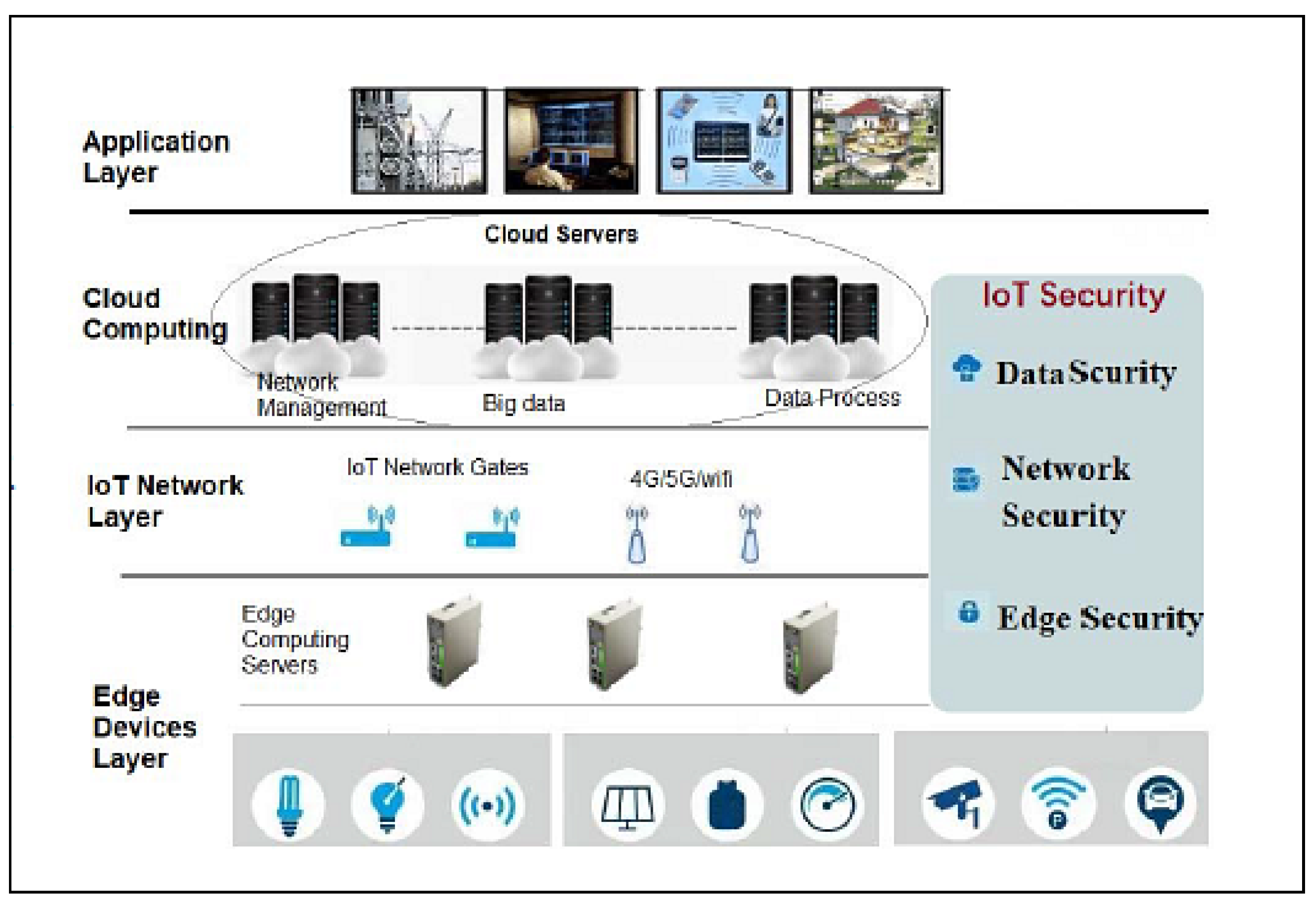
Designing an efficient network intrusion detection model is a crucial step in ensuring data security. Correspondingly, designing the efficient network intrusion detection model requires to understand the architecture of IOT systems The IOT system is made up of various components like IOT devices, computation servers, Internet devices, and wireless devices. There are six layers in this architecture, and the application service layer is the most prominent one. this architecture mainly consists of six layers: 1) application service layer; 2) information integration layer (cloud computing); 3) network layer; 4) information access layer; 5) information acquisition layer (edge computing); and 6) edge device layer, whose basic framework is displayed in Figure (2) [37].
Figure 2.
Architecture of IOT system [37].
Figure 2.
Architecture of IOT system [37].
IDS is a technology which ensures security by continuously scanning network and host traffic for any suspicious activity, which may breach security policy and may jeopardize data confidentiality as well as integrity. Feature engineering plays a crucial role in extracting relevant network information for Machine Learning (ML) based Intrusion Detection Systems (IDSs) [38]. one of the most common attacks in wireless networks including IOT is denial of service; a type of attack whose goal is to disrupt the service integrity of a network node. Hence, proposing an efficient intrusion detection system that can inspect and eliminate malicious nodes in the network and in turn improve network performance through continuous traffic monitoring is highly important [8]. Neural networks and Support Vector Machines (SVM) have proven to be powerful classifiers for network intrusion detection [9]. An evolutionary intelligence and RNN-based attack detection method for IOT networks (IOT - RNNEI) is proposed in this paper to address the mentioned issues. the proposed model uses the combined Grasshopper Optimization Algorithm (GOA) [10] and the Sine Cosine optimization algorithm (SCA) [11] to improve the weights of the random neural network, which has high search accuracy. It's a commonly accepted fact that using a lightweight random neural network solution is effective in identifying attacks on IOT networks. In the standard random neural network method, the weight adjustment is done by the gradient descent method, which places it in the local optimum and does not reach the optimal state for the network weight, however in the proposed framework, we reach the global optimum using meta-heuristic algorithms, which are the optimal weights of the neural network. In general, the purpose of this research is to boost the accuracy of the neural network by adjusting the architecture of the weights of this method, and for this purpose, the strong search power of the combined algorithm of grasshopper and sine cosine has been used. The paper's innovations can be summarized in the following way:
1. The random neural network was upgraded and enhanced using a combined algorithm of grasshopper and sine cosine optimization in this study, this process aims to reduce training time and improve the model's robustness.
2. A unique hybrid optimization structure is outlined in this paper, by adjusting weights and determining the architecture of random neural network types using a combination of sine cosine optimization and GOA algorithms, this framework enhances the accuracy of intrusion detection in IOT networks.
3. To address early convergence in a local minimum of the squared error function that adjusts the weights of the standard random neural network, this paper proposes utilizing a combined evolutionary algorithm involving sine cosine and GOA to approach the minimum of the error square function.
The article continues with the following structure: Section 2 offers a review of pertinent research. In Section 3, you will find a description of grasshopper and sine cosine algorithms. Section 4 proposes the algorithm and methodology; Section 5 demonstrates the implementation and evaluation of the proposed model; Finally, in Section 6 we present the conclusion and future work.
2. Related Works
This section focuses on the research conducted in developing attack detection systems in IOT applications, which includes various machine learning methods on different datasets in this field. ET-DCANET, a highly efficient hierarchical intrusion detection model, was introduced by Xin Yang et al [7]. In this model, the extreme random tree algorithm was utilized to meticulously choose the optimal feature subset. Subsequently, the dilated convolution and dual attention mechanism (channel attention and spatial attention) were introduced, along with a plan to transition from overall learning to detailed learning by decreasing the expansion rate of cavity convolution. It was discovered that this model has an accuracy of 99.85%. Wang et al [12] introduced a network intrusion detection model based on deep learning (DL). This model sought to boost detection accuracy through feature extraction from spatial and temporal aspects of network traffic data. The aim of the model was to amplify the minority class samples, handle data imbalance, and enhance the accuracy of network intrusion detection. The model achieved an accuracy of 97.47%. elsewhere in their work, ARINDAM SAKAR et al [13] proposed intrusion detection system within a Block Chain framework that leverages federated learning (FL) and an artificial neural network (ANN)-based key exchange mechanism. A. SUBRAMANIAM et al [14] Intrusion Detection System using Hybrid Evolutionary Lion and Balancing Composite Motion Optimization Algorithm espoused feature selection with Ensemble Classifier (IDS-IOT Hybrid ELOA-BCMOA-Ensemble-DT-LSVM-RF-XGBOOST) propose for Securing IOT Network. Accuracy of this model was achieved 94.47%. G. SATHISH Kumar et al [15] In their study, SATHISH Kumar et al [15] introduced a statistical differential privacy-deep neural network (DNN - SDP) algorithm to protect sensitive personal data. The input layer of the neural network received both numerical and categorical human-specific data. The statistical methods weight of evidence and information value was applied in the hidden layer along with the random weight () to obtain the initial perturbed data. This initially perturbed data were taken by Laplace computation based differential privacy mechanism as the input and provided the final perturbed data. DNN-SDP algorithm provided 97.4% accuracy. In [16], the main goal was to develop suitable models and algorithms for data augmentation, feature extraction, and classification. The proposed TB-MFCC multi-fuse feature consisted of data amplification and feature extraction. In the proposed signal augmentation, each audio signal used noise injection, stretching, shifting, and pitching separately, where this process increased the number of instances in the dataset. The proposed augmentation reduced the overfitting problem in the network. The suggested Pooled MULTIFUSE Feature Augmentation (PMFA) with MCNN & A-BILSTM enhanced the accuracy to 98.66 %. The proposal by SATHISH Kumar et al [17] outlines a homomorphic encryption scheme that utilizes the privacy chain, the weight of evidence, and the information value of the statistical transformation method. This scheme is designed to safeguard the user's private and sensitive information. The proposed STHE algorithm ensures that perturbing numerical and categorical values from multiple datasets does not impact data utility. Elsewhere, in [18] a new model and lightweight forecasting model was proposed using time series data from the KAGGLE website. The obtained dataset was then processed with the help of deep learning techniques. The Long Short-Term Memory (LSTM) algorithm was used to produce better results with higher accuracy when compared with other deep learning methodologies. In [19], A model for the class imbalance problem was addressed using Generative Adversarial Networks (GANs). Accordingly, an equal number of train and test images was considered for better accuracy. The prediction accuracy was enhanced by Multi piled Deep Convolutional Generative Adversarial Network (DCGAN). In [20] An automatic number plate recognition (ALPR) system provided the vehicle's license plate (LP). The computer vision area considered the ALPR system as a solved problem. The algorithm applied in the proposed methodology was Convolution Neural Network (CNN). In [21] A quadratic static method was used to find the correlation between features, enhancing the dimensionality reduction in the dataset, where deep over-optimization and genetic hyper-learning model (DHO-GML) were applied to efficiently perform the classification by selecting the optimized model. The proposed model produced an accuracy above 99%. In another research, [22] Created design and computation to support fine-tuned static allocation scheduling for distributed computing space with dynamic distribution of virtual machines. The design coordinated delicate continuous assignment planning calculations, particularly expert hub and virtual machine hub plans. In [23], was model used to increase cognitive efficiency in Artificial General Intelligence (AGI), thereby improving agent image classification and object localization. This system, which used RNN and CNN, would enable any user to do creative work using the system model. The system model took in the sample input and produced the output based on the input given. P.R. KANNA and P. SANTHI [24] presented an efficient hybrid IDS model built using Map Reduce-based optimized Black Widow short-term convolutional-long-term memory (BWO-CONV-LSTM) network. This model was used for intrusion detection in online systems. The first stage of this IDS model involved the feature selection by the Artificial Bee Colony (ABC) algorithm. The second stage was the hybrid deep learning classifier model of BWO-CONV-LSTM on a Map Reduce framework for intrusion detection from the system traffic data. P Rajesh KANNA and P SANTHI [25] proposed a high-accuracy intrusion detection model using an integrated optimized CNN (OCNN) model and hierarchical multiscale LSTM (HMLSTM) to effectively extract and learn SPATIO-temporal features. The proposed intrusion detection model performed pre-processing plus feature extraction through network training and network testing together with final classification. In [26], a new DOS attack detection system was introduced, which was equipped with the previously developed MCA technique and EMD-L1. The technique used previously helps extract the correlations between individual pairs of two distinct features within each network traffic record and detects more accurate characterization for network traffic behaviors. The recent technique facilitates our system to be able to effectively distinguish both known and unknown DOS attacks from authorized network traffic. In [27], the authors offered a system that recommended the right crops for the region and the right fertilizers for the crops to farmers based on soil measurements, all based on past years' yield history. This agricultural yield forecast and fertilizer recommendation would employ machine learning methods. The random forest algorithm and the K-means clustering algorithm proved to be successful in predicting crop suitability and recommending FERTILISER. The dataset for the Salem region contains a number of factors that are used for this purpose. The approach in [28] utilized deep learning technology to detect leaf diseases through the Recurrent Neural Network (RNN) algorithm. About 53,000 images of infected and healthy leaves, showcasing fruits and vegetables such as apple, orange, strawberry, and more, make up the dataset. The neural network was trained to increase accuracy in predicting efficient outputs. Elsewhere [29] conducted a study on a water quality monitoring system to make water quality predictions with a machine learning system. The aim of this study was to create a water quality prediction model using an Artificial Neural Network (ANN) and time-series analysis. The specific data and investigation goals will determine the chosen prediction model. In [30], researchers studied the use of feature reduction, feature selection, and machine learning models to detect attacked traffic in IOT industrial networks. They explored the combination of PSO and PCA with MARS or GAM machine learning models. in another research, [31] proposed framework for advancing an explicit sprayer arrangement. The created gadget aimed to reduce the use of pesticides by spraying individual targets explicitly and by setting the separation of spray items based on the target. A sharp mechanical structure for spraying pesticides in cultivation field for controlling the robot by the use of a remote choice rather than manual completion of yields shower tests, would reduce the prompt prologue to pesticides and the human body, while also decreasing pesticide harm to people and improving age adequacy. In [32], the authors tried to diagnose heart disease through Support Vector Machine (SVM) and Genetic Algorithm (GA) as a data analysis approach. AI methodologies were utilized during this work to influence crude data providing novel insights into coronary artery disease. In their proposal, ANITTHA GOVINDARAM and JEGATHEESAN A [33] presented FLBC-IDS, a technique that utilizes HFL, HYPERLEDGER BLOCKCHAIN, and EFFICIENT Net for effective intrusion detection in IOT environments. HFL empowers the FLBC-IDS model to enable secure and privacy-preserving model training on a wide range of IOT devices, leading to decentralized data privacy and optimized resource utilization. presented an accuracy of 98.89%, recall of 98.044%, F1-score of 98.29%, and precision of 98.44%. They created a model in [34] that combines federated learning with distributed computing resources and BLOCKCHAIN decentralized features to introduce an intrusion detection framework called IOV-BCFL. It was capable of distributed intrusion detection and reliable logging with privacy protection. Elsewhere, [35] introduced a model called MP-GUARD, a novel framework which used software-defined networking (SDN), machine learning (ML), and multi-controller architecture to address intrusion detection challenges. MP-GUARD tackles multi-pronged intrusion attacks in IOT networks by offering real-time intrusion detection, collaborative traffic monitoring and multi-layered attack mitigation. This model achieved exceptional performance with 99.32% accuracy, 99.24% F1 score, and 0.49% false positive rate. In another study, [36] discussed a new intrusion detection system that approached big data management. Intrusion detection was done by a hybrid model, fusing the long short term memory and optimizing convolutional neural network (CNN). Then, the optimization-assisted training algorithm called elephant adapted cat swarm optimization (EA-CSO) was proposed which would tune the optimal weights of CNN to enhance the performance of detection. In [43], a new light intrusion detection system was designed in two phases using swarm intelligence based technique. In the first step, the basic features were selected using the particle swarm optimization algorithm considering the unbalanced data set. The ant colony optimization algorithm was used in the second phase to extract information-rich and unrelated features. In addition, genetic algorithm was employed to fine-tune each detection model. The accuracy of the model was 97.87%. In [44], an advanced local search locus algorithm was proposed based on recurrent federated network (RFN-ELG). Datasets such as UNSW-NB15 and MQTT-IoT-IDS2020 dataset were used to determine IIOT performance through two different phases, i.e. data preprocessing phase as well as attack detection phase. In a different study, [45] proposed a client selection method using clustering to identify malicious clients by analyzing their run time. This was paired with a trigger-set-based encryption system for client authentication, achieving a model accuracy of 99.8%. A comparison of the various approaches for analyzing the research gap is presented in Table 1.
Research Gap
Table 1 lists current techniques like FL, SVM, PSO, ML, and DL for IOT attack detection. Despite this, the techniques show low convergence speed, detection rate, and efficiency. to overcome these issues, an evolutionary intelligence and RNN-based attack detection method is proposed to detect attacks in IOT networks (IOT - RNNEI). The research gaps are illustrated as follows:
The detection efficiency is enhanced through the implementation of the grasshopper and sine-cosine optimization algorithm, which integrates local and global search strategies.
Attack detection: Existing intrusion detection methods can have a low accuracy rate and even a high False Alarm Rate (FAR). Hence, our proposal aims to enhance the detection performance rate in the Internet of Things network by introducing a new model for intrusion detection.
3. Preliminary Concept
Basic concepts, including the Grasshopper Optimization Algorithm and the Sine Cosine Optimization Algorithm, are discussed in this section.
- Grasshopper Algorithm
One of the new evolutionary algorithms is the Grasshopper Optimization Algorithm (GOA), inspired by the behavior of grasshoppers. Nature-inspired algorithms logically divide the search process into two parts: exploration and operation. In exploration, search agents are encouraged to make random movements, while in the operation stage, they tend to make local movements around their location. These two actions, along with the search for the target, are naturally performed by grasshoppers. Thus, an attempt has been made to find a way to mathematically model this behavior, which is presented in the following mathematical specifications. Formula (1) [10] illustrates the mathematical model used to simulate the behavior of grasshoppers:
Here, represents the position of the grasshopper, denotes social interaction, is the gravitational force applied to the grasshopper, , and indicates the wind direction. The value of , meaning social interaction for grasshopper is calculated according to Formula (2) [10].
Where, represents the distance between the grasshopper and the grasshopper and is calculated using Formula (3) [10].
The function () defines social force pressure in Formula (2) with () as a unit vector from one grasshopper to another. the grasshopper. () The function , defining the social force, can be calculated using Formula (4) [10].
where represents the intensity of attraction and denotes the scale length of attraction. The function is illustrated in Figure (3) to reveal how it affects the social interaction (attraction and repulsion) of grasshoppers.
In Figure 3, repulsion is observed between 0 and 2.079 in the distance range of 0 to 15. The distance of 2.079 between grasshoppers is called the comfort zone, with no attraction or repulsion. Figure 3 demonstrates attraction increasing until around 4 from a distance of 2.079. Changing the parameters, and in Formula (4) leads to different social behaviors in artificial grasshoppers. To observe the impact of these two parameters, the function in Figure 4 with different values of and in Formula (4) will result in various social behaviors in artificial grasshoppers.
Figure 4 reveals that the parameters and significantly alter the comfort, attraction, and repulsion regions. Note that the attraction or repulsion regions are very small for certain values (for example, = 1 and = 1). In simulations, values of = 1.5 and = 0.5 have been used. A conceptual model of interactions between grasshoppers and the comfort zone using the function is depicted in Figure 5.
The function () distinguishes between repulsion, attraction, and comfort zones for grasshoppers, showing values close to zero for distances beyond 10 in Figure 3 and Figure 4. As a result, this function lacks the ability to produce strong forces between separated grasshoppers. In order to tackle this problem, the separation between two grasshoppers is represented on the range [1,4]. The illustration in Figure 3 displays the function's shape within this interval. Studies have demonstrated that Formula (1) is not suitable for congestion and optimization algorithm simulations due to its impact on exploration and exploitation within the search space near a solution. The model has been used to tackle congestion in an unoccupied space. Consequently, Formula (5) [10] is applied to simulate grasshopper interactions during congestion.
where is the upper bound in dimension , denotes the lower bound in dimension , is the value in dimension of the target (the best solution seen so far), and is a reduction constant for minimizing the comfort, repulsion, and attraction regions. In this equation, is derived from Formula (4), while the parameters of gravity () and wind direction () are not considered. The behavior of grasshoppers in a space using Formula (5) is depicted in Figure 6.
In Figure 6, a total of 20 artificial grasshoppers are utilized for movement within a time exceeding 10 units. Figure 6 demonstrates how Formula (5) brings the initial random population closer together to form a unified and organized congregation. After 10-time units, all grasshoppers reach the global optimum region and cease further movement. Formula (5) defines the next position of a grasshopper based on its current position, the target position, and the positions of all other grasshoppers. Note that the first component in this relation considers the position of the current grasshopper concerning other grasshoppers. In essence, we consider the status of all grasshoppers to define the positions of search agents around the target. This is a different approach compared to the Particle Swarm Optimization (PSO) algorithm. In PSO, there are two vectors for each particle: the position vector and the velocity vector. However, in the GOA, there is only one position vector for each search agent. Another main difference between the two algorithms is that PSO updates the particle position according to the current position, personal best experience, and public best experience. However, the GOA algorithm updates the position of the search agent based on its current position, the general best answer, and the positions of other Grasshoppers. It is also noteworthy that the adaptive parameter has been used twice in Formula (5) for the following reasons [10]:
- The item positioned first on the left bears a strong resemblance to the inertia weight () used in the PSO algorithm. It decreases the movement of grasshoppers towards the target. To clarify, this parameter maintains a balance between exploring and exploiting the target.
- The second variable decreases the areas of attraction, repulsion, and comfort among grasshoppers. Consider the component in Formula (5), where linearly reduces the space between grasshoppers that should explore and exploit.
In Formula (5), the internal leads to a proportional reduction in attraction/repulsion force between grasshoppers with each iteration of the algorithm, while the external diminishes the search coverage around the target with an increase in the number of algorithm iterations. In summary, the first part of Formula (5) considers the positions of other grasshoppers and simulates interactions among grasshoppers in nature, while the second part simulates the tendency to move towards a food source in grasshoppers. Additionally, parameter simulates a decline in the speed of grasshoppers as they approach a food source and eventually consume it. To maintain a balance between exploration and operation, parameter needs to fall with a rise in iterations during the algorithm. The coefficient reduces the comfort zone proportionally with the number of iterations and is calculated using Formula (6) [10].
where is the maximum value, shows the minimum value, indicates the current iteration number, and represents the maximum number of algorithm iterations. In simulations, is considered as 1 and as 0.00001. The impact of this parameter on the movement and convergence of grasshoppers is illustrated in Figure 7.
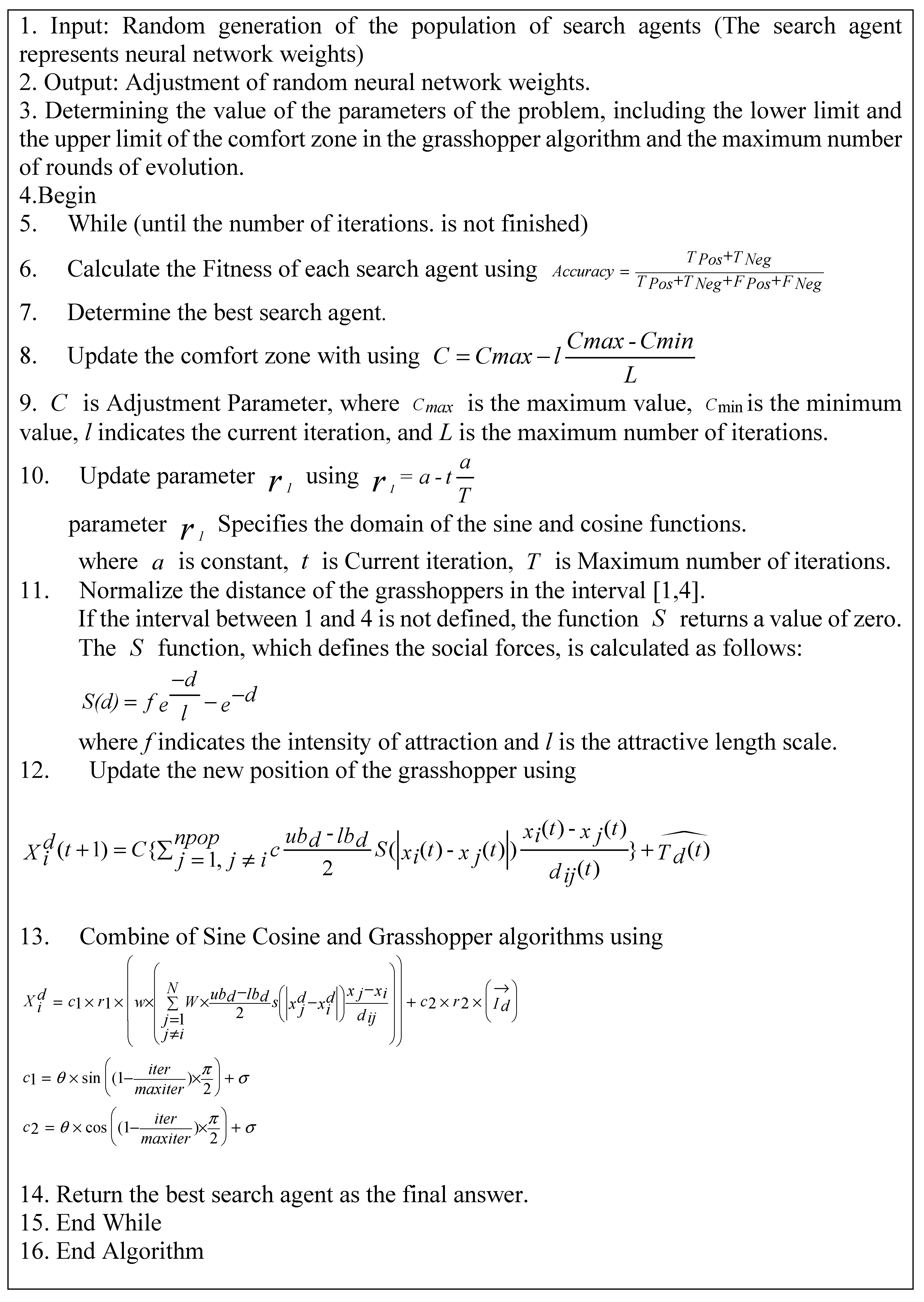
Experiments have been conducted on fixed and moving targets to assess the performance of the GOA in understanding how the movement of grasshopper congregations towards the optimal solution of a problem occurs. The history of grasshopper positions over 100 iterations in Figure 7 demonstrates that the congregation gradually converges towards a fixed target in a two-dimensional space, a behavior attributed to the reduction of the comfort zone by factor . It is also shown that the congregation effectively follows a moving target, and this is why the last component of formula (5) is , in which the grasshopper is pushed towards the target. These behaviors assist the GOA algorithm in avoiding rapid convergence towards a local optimum, ensuring that grasshoppers converge towards the target as much as possible, a behavior being crucial during exploitation. The mathematical model presented for the GOA requires grasshoppers to gradually converge towards the target over the course of algorithm iterations. However, in real search spaces, there is no specific target since we do not know exactly where the global optimum, i.e., the main target, is located. Therefore, at each optimization stage, we will find a target for the grasshoppers. In the GOA, it is assumed that the best grasshopper during algorithm execution (the grasshopper with the best objective function value) is the target. This helps the algorithm store the most promising target in the search space at each iteration and compels grasshoppers to move toward this target. This is performed with the hope of finding a better and more accurate target as the best approximation for the global optimum in the search space [10]. You can see the pseudocode of the grasshopper algorithm in Figure 8.
The GOA has a strong search mechanism in the sterile problem space, and in the optimization of high-dimensional functions, it has shown a high accuracy in reaching the global optimum. Due to the collective movement of the grasshoppers to a region of space where the global optimum lies, the optimality of the problem is found with greater accuracy. which makes the convergence accuracy of this algorithm, the dependence of this algorithm on the number of search agents and the other hand the collective movement of grasshopper to the better area of the search space causes, some points of the search space (if there are few search agents) will not be properly explored. This will cause premature convergence to the local optimum; further, in this algorithm, the number of agents is fixed until the end of the algorithm iteration, which will elevate the number of function evaluations. This is because at the beginning of the work, the algorithm needs the right number of search factors and strong exploration, but as the end of the algorithm iterations approaches, extraction will be needed, and for optimal extraction (convergence to optimality), not all search factors may get involved. Also, the important parameter of this algorithm is the comfort zone, which in this algorithm falls linearly and according to the iterations of the algorithm, and in which the rate of convergence and the state of the grasshoppers in the search space are not included [10].
- Sine Cosine Optimization Algorithm
The Sine Cosine Optimization Algorithm (SCA) is an elitist population-based method that has demonstrated high extraction power and precise convergence, leading to achievement of the exact optimal point even in high-dimensional functions. This algorithm addresses both exploration and exploitation in optimization and aims to find the global optimum of the problem. In this algorithm, the best solution always represents the destination for search waves. Thus, search waves do not deviate from the primary optimum of the problem. Further, the fluctuating behavior in this algorithm allows it to search the search space around the optimum of the problem well, regardless of the difference between algorithms in the field of random population based optimization, with the optimization process being divided into two common phases: exploration versus exploitation. The following position update equations for both phases are specified using Formula (7) [11].
Where is the position of current solution in dimension at iteration, represent random numbers, position of the destination point in dimension, and indicates the absolute value. These two equations are combined to be used as follows [11].
Where is random number in ; there are four main parameters in SCA: .
denotes the new coordinates of the search wave and represents the previous coordinates of the search wave and shows the coordinates of the best solution found, which is considered as the destination. if less than 1, move towards the destination point, and if it is greater than 1, move away from the destination point. Formula (9) displays the effect of the parameter on the movement of waves in the sine-cosine algorithm. Formula (10) shows the effect of the parameter on the discovery and extraction of the sine-cosine algorithm. Also, the effect of the resolution parameter is shown in Figure 9.
Where is the current iteration, denotes the maximum of iterations, and is constant.
Parameter is used to model oscillatory movement which varies within . Figure (11) illustrates the impact of parameter on wave movement in the sine cosine optimization algorithm. You can see the effect of the parameter clearly in Figure 11.
serves as a weight for the destination; if it is considered greater than 1, a larger step towards the destination is taken, and if it is less than 1, a smaller step is taken towards the destination. is a random variable between 0 and 1 The optimal solution to the problem is obtained by completing the final number of iterations of the algorithm and selecting the best-found solution, which is determined by a random variable between 0 and 1 that switches between sine and cosine movements. You can see the pseudocode of the sine-cosine algorithm in Figure 12.
4. Proposed Method for Detecting Attacks in IOT
Network intrusion detection benefits from the superior performance of hybrid models. The limitation of single CNN or RNN models is the singular feature extraction dimension, resulting in relatively worse classification outcomes. residual network structures offer significant advantages in a variety of tasks. The recent RESNEST [12] model has become popular because of its ability to be applied to different tasks. however, we know that Random Neural Network is a suitable solution for attack detection in Internet of Things networks [6]. Meanwhile, adjusting the weights of random neural networks is directly related to their classification accuracy. Also, by adjusting the internal parameters of neural networks, they reach high accuracy in classification. So in our proposed framework, the internal parameters and architecture of the random neural network are adjusted using meta-innovative algorithms to enhance its classification performance and accuracy. Indeed, adjusting the weights and architecture of the neural network aims to improve the classification accuracy. Note that the sine cosine algorithm has a high exploration power and the grasshopper algorithm has a high exploitation power, and the combination of these two algorithms seems to be able to search the search space more accurately. Indeed, in the standard random neural network, gradient descent is used to adjust the weights of the network, and to obtain the minimum square of the network error, the weights are adjusted as backpropagation of the error. Gradient descent is an optimization method through derivative calculation which reaches early convergence to a local minimum at the first minimum in the optimization functions, including the error square function in the random neural network, and cannot converge to the minimum point of the function. Thus, the combined evolutionary algorithm of sine cosine and grasshopper is used to converge to the minimum point of the error square function in this random neural network. We also know that one of the criteria for evaluating the proposed approach is the accuracy of the intrusion detection system. According to the architecture of the proposed method shown in Figure (15), the output of the neural network (proposed model) is pattern recognition. So, by optimally adjusting the weights of the neural network, the accuracy of pattern recognition increases, and ultimately leads to heightened accuracy of the accuracy of pattern recognition in IOT networks improves by optimally adjusting neural network weights, resulting in enhanced attack detection and intrusion identification. Figure (15) illustrates the architecture of the metaheuristic optimization algorithms-based IOT network intrusion detection model proposed in this article.
4.1. Dataset Description
An open-source dataset named DS2OS was obtained from KAGGLE [40]. This is one of the new generations of IOT datasets for evaluating the fidelity and efficiency of different cybersecurity applications based on machine/deep learning algorithms. The dataset consists of 357952 samples and 13 features. It has 347935 normal data values and 10017 anomalous data values, with 8 classes. Two features ``Value'' and ``Accessed Node Type'' have 2500 and 148 missing values, respectively. Indeed, in this paper, the dataset consists of 260,000 samples with eleven features (Source Address, Source Type, Source Location, Destination Address, Destination Type, Destination Location, Accessed Node Address, Accessed Node Type, Operation, Value, Timestamp). The dataset is split into 70% for training and 30% for testing the model. The input characteristics are labeled X1 through X11. The dataset is split into a training set of 80% and a test set of 20%. in order to apply the suggested model, this dataset includes a total of 13 characteristics. Column 1, known as "Source ID," does not play a significant role in predicting attacks. Consequently, this column was excluded in the preprocessing process. Column 13 serves as an output feature denoting "Normality." As a result, the RNN (Random Neural Network) was fed with 11 features as input. In Table 2 [6], you can find a concise summary of the attacks present in the DS2OS dataset.
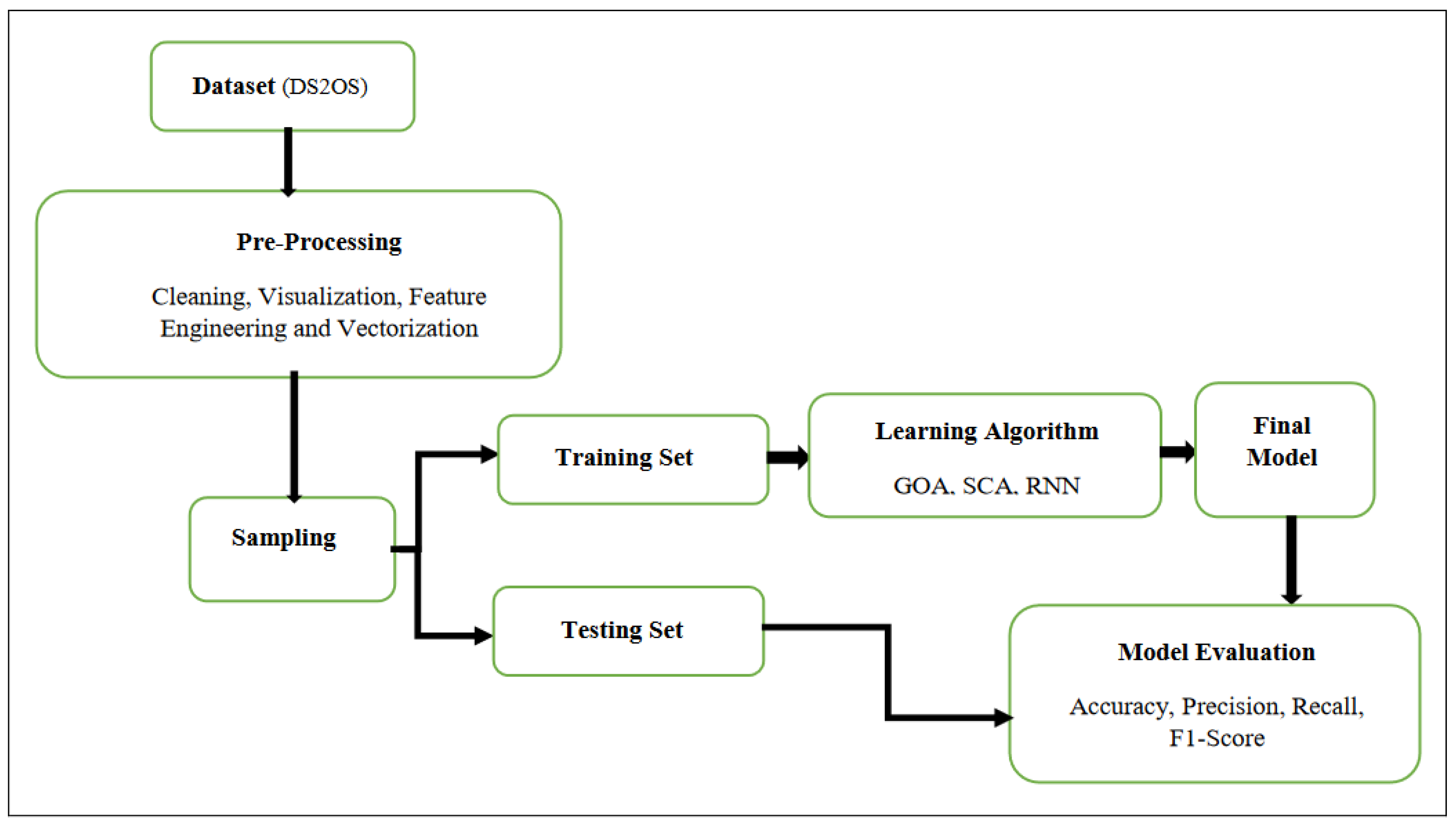
Figure 13.
The IOT network intrusion detection model uses metaheuristic optimization algorithms and RNN in its structural flow chart.
Figure 13.
The IOT network intrusion detection model uses metaheuristic optimization algorithms and RNN in its structural flow chart.
4.1.1. Dataset Preprocessing
Machine learning research requires good and comprehensive data analysis. The first step is to arrange data in such a configuration that they will be compatible with the input of any ML algorithm. This dataset contains missing values in two feature columns “Accessed Node Type”. The “Accessed Node Type” feature column contains 148 “NAN” values. This feature includes categorical data, so if we remove these 148 rows, then there will be a great possibility of losing some valuable information. Therefore, the “NAN” value is replaced with the “Malicious” value. Some data present in the “Value” column Are also unassigned. These unexpected values are replaced with some meaningful values. True, False, Twenty, and None are replaced with 1.0, 0.0, 20.0, and 0.0, respectively. In the next step, the first and most important task is to identify the type of features. This dataset contains numerical and categorical data. Numerical data are further classified into continuous and discrete values. Categorical data are classified into ordinal and nominal values. In the dataset, all columns contain categorical nominal variables, except “Value” and “Timestamp”. These two columns consist of continuous numerical variables. The next important step is to convert categorical data into feature vectors. In this research, categorical data are converted into feature vectors via label encoding. In the dataset, most of the features consist of nominal categorical values, so the advantage of label encoding is that the number of features will remain the same. Label-encoded data are easy to fit in ML algorithms, and the processing time is shorter than that of one-hot encoding [6].
4.1.2. Data Balancing
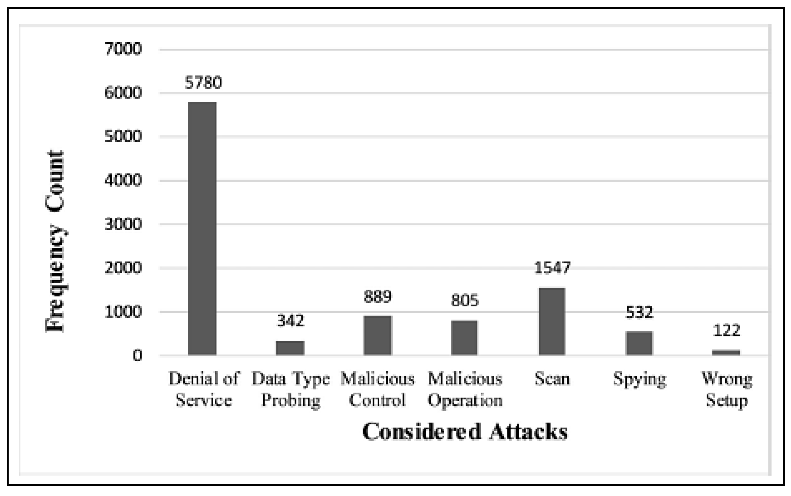
An imbalanced data distribution in network intrusion detection tasks can lead to decreased effectiveness for certain categories, despite good performance on the majority category. The decline in recall for some categories and overfitting the majority category may affect generalization. Tabular datasets are commonly utilized in network intrusion detection. The dataset used in this article is also tabular. DS2OS [40] can model and sample the distribution of data. The frequency-based sampling of data during training is determined by the logarithm of each category. As a result, DS2OS can uniformly examine all possible discrete values. Two feature columns in this dataset have missing values in the "Accessed Node Type". Within the "Accessed Node Type" feature column, there are 148 occurrences of "NAN" values. Since this feature contains categorical data, eliminating these 148 rows could result in losing valuable information. Thus, the "NAN" value is substituted with the "Malicious" value. Some data in the "Value" column remains unassigned. These surprising values have been substituted with more meaningful ones. True, False, Twenty, and None are substituted with 1.0, 0.0, 20.0, and 0.0, in that order. As a result, this paper uses the dataset to create samples focusing on specific categories, addressing data imbalance and tackling unbalanced data issues. The distribution of diverse attacks in the dataset is laid out in detail in Figure (14).
Figure 14.
Statistics of considered attacks in the DS2OS dataset [41].
Figure 14.
Statistics of considered attacks in the DS2OS dataset [41].
4.2. Model Structure
Based on collective intelligence and neural network principles, this paper presents an intrusion detection technique for IOT networks. as depicted in Figure (15), the proposed model includes several sections, with each section discussed separately.
Figure 15.
Architecture of the proposed method.
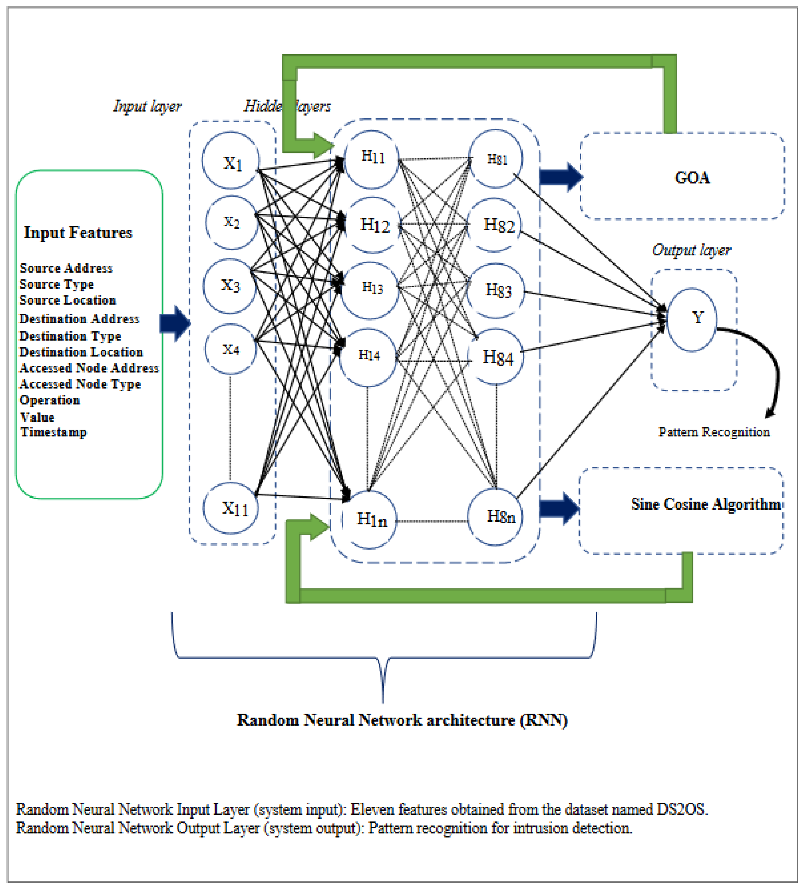
In this paper, the DS2OS dataset [40] consists of 260,000 samples with eleven features (Source Address, Source Type, Source Location, Destination Address, Destination Type, Destination Location, Accessed Node Address, Accessed Node Type, Operation, Value, Timestamp). The dataset is divided into 70% for training and 30% for testing the model. These input features are named X1, X2, to X11. The dataset is split into a training set and test set, with a ratio of 80% and 20%, respectively. Eleven features were used as input for the RNN.
- Section 2: Random neural network architecture
In this section, we briefly explain the architecture of the random neural network. The technique for attack detection in IOT systems, such as the ANN and the Random Neural Network (RNN) is also inspired by the human brain. RNN contains 1 input layer, 8 hidden layers, and 1 output layer. The input layer assigns weights plus biasness values and forwards these data to hidden layers for further processing [6]. Learning is very important in hidden layers as it plays a critical role in predicting the output from real features. Hidden layers transfer this information to the output layer for suitable output generation. After learning, the trained model is used to predict attacks by using a test set.
- Section 3: Adjusting the architecture of the Lightweight random neural network by using the sine cosine optimization and GOA combined algorithm in terms of the number of hidden layers and neurons of each layer.
The sine cosine optimization and GOA combined algorithm has high extraction power and accurate convergence. This contributes to achieving the optimal exact point even in high-dimensional functions. In this algorithm, the best answer is always the motion indicator for search agents. Therefore, the combined chain of Sine Cosine and GOA does not deviate from the original optimality of the problem. Also, the various movement behaviors in this algorithm allow it to search the search space around the optimality of the problem well and have good accuracy of obtaining the optimality. The proposed framework (combination of sine cosine and grasshopper algorithms) is shown using Equations (10) and (11).
The range of is between 2.5 and 0.5 while ranges from 0.5 to 2.5. The values of and c2 specify how distant the searching should be outwards from or towards the target. The dimensions of and are altered adaptively using the sine cosine algorithm ( SCA ) as given in Formula (11).
where θ and σ are constants (θ = 2, σ = 0.5). The theoretical model of SCA (c1 and c2) The random numbers r1 and r2 between (0, 1) provide the movement with a direction (or region) of the current position either within the solution region and target point or outside of both. The w is the inertia weight factor similar to c. controlling the movement of the grasshopper, which is calculated as illustrated in Equation (6). Significantly, the random perturbation (r1 and r2) makes sudden changes in the solution leading to the avoidance of the local minima while reducing the convergence speed towards the global optimum. Contrarily, the SCA coefficients yield high convergence and coverage for optimization. Figure (16) displays the structure of a search agent to find the number of hidden layers and neurons in each layer of the neural network.
Figure 16.
Structure of a search agent.
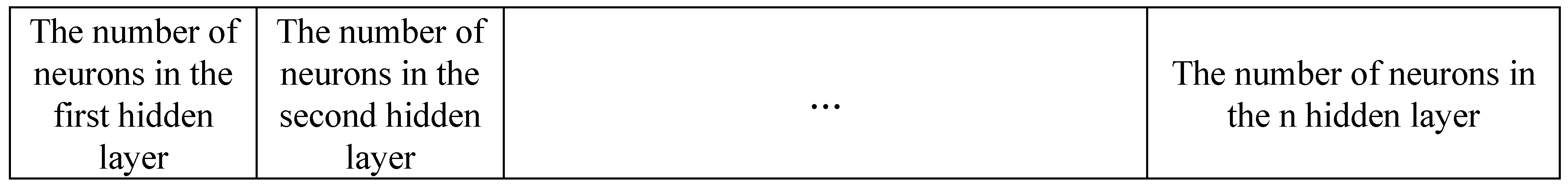
Stage 1
1. A search agent is an array with a specified number of cells (the number of non-zero cells in the array is equivalent to the hidden layers of the network), where the number inside each array indicates the number of neurons in that hidden layer. Figure (17) illustrates an example of a search agent.
Figure 17.
Sample of a search agent.

As shown in Figure (17), the number of hidden layers of the random neural network is equal to 8 and the number of neurons in each hidden layer of the neural network is equal to: 5, 2, 4, 7, 1, 8, 2, and 4 in order.
Stage 2
1. Using the grasshopper and sine cosine algorithms, the best search agent is obtained, which is shown in Figure (18).
2. The fitness function is the classification accuracy; using Formula (12), the fitness function of each search agent is determined.
Where is The number of records whose actual class is negative and the classification algorithm correctly identifies them as negative. denotes the number of records whose actual class is positive and the classification algorithm correctly identifies them as positive. shows the number of records whose actual class is negative but the classification algorithm incorrectly identifies them as positive. Finally, reflects the number of records whose actual class is positive but the classification algorithm incorrectly identifies them as negative.
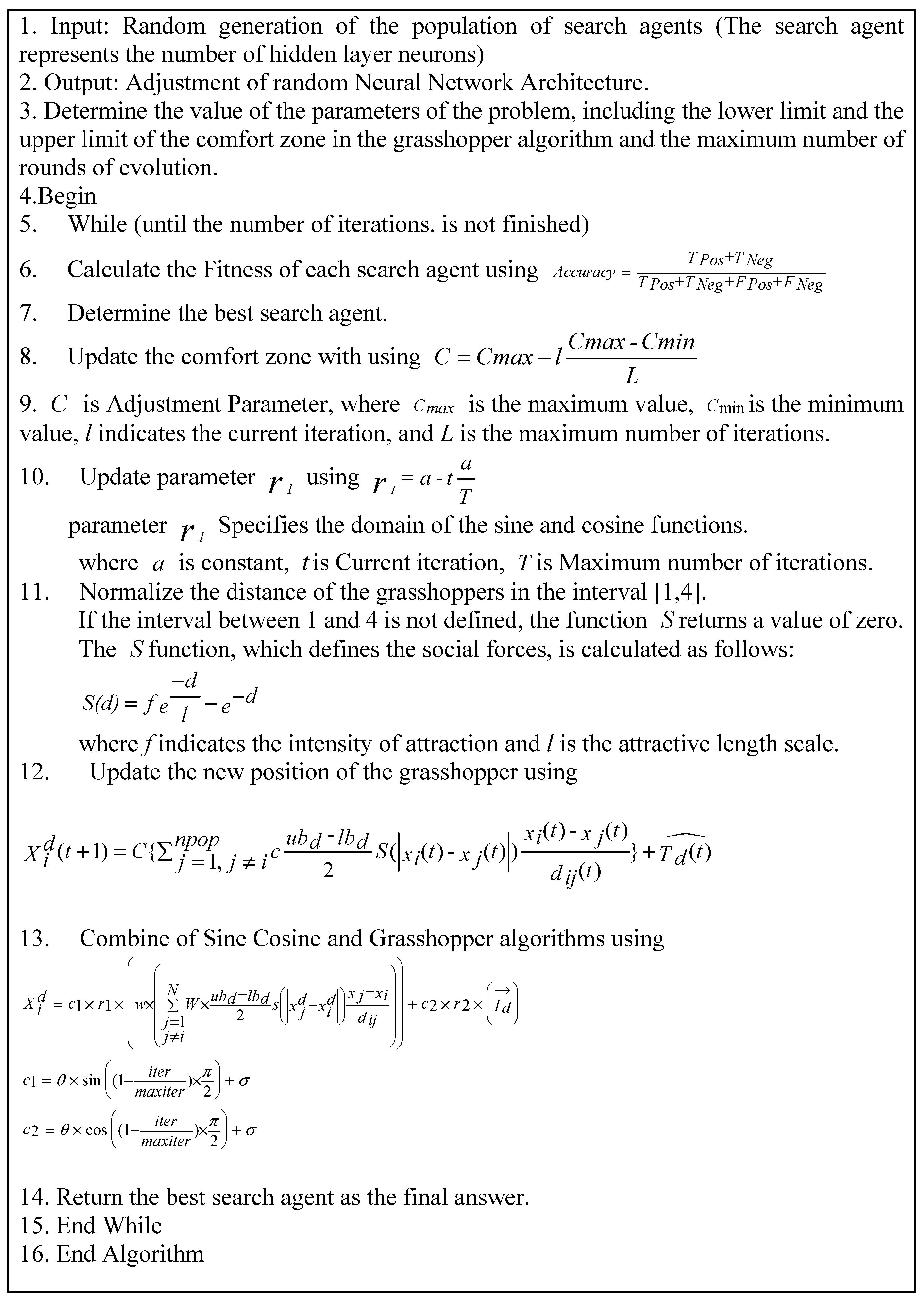
Figure 18.
Adjustment of random neural network architecture pseudo-code.
- Section 4: Adjusting the weights of the lightweight random neural network using the sine cosine optimization and GOA combined algorithm
According to the random neural network architecture (RNN), neurons are connected in different layers. These neurons have excitation and inhibition states, which depend on the potential of a received signal. The state of neuron at time is represented by ; Neuron will remain in an idle state until the value of . To go into an excited state because is considered a nonnegative integer. In the excited state, a neuron transmits an impulse signal to another neuron at the transmission rate of . The transmitted signal can be received by neuron as a positive signal or a negative signal with the probabilities of and respectively. Furthermore, the signal can also leave the network with a probability of [6].
The weights of neurons and are updated as:
In the RNN, the probability of the signal is determined by a Poisson distribution. Thus, for neuron , positive and negative signals are represented by the Poisson rate and respectively, which can be mathematically described as:
The output activation function can be described as:
The transmission rate is represented by , which can be calculated using Equation (17) [6].
In Equation (17), is the gain of the firing rate. During the training of the RNN, probabilities of positive and negative weights are updated, which can be described by Equation (18) [6].
Indeed, in the standard random neural network, gradient descent is used to adjust the weights of the network, and to obtain the minimum square of the network error, the weights are adjusted as error backpropagation. Gradient descent is an optimization method through derivative calculation that reaches premature convergence to a local minimum at the first minimum in the optimization functions, including the error square function in the random neural network, and cannot converge to the minimum point of the function. The error function is described in Equation (19) [6].
Where represents the state of output neuron . The actual differential function predict output values are represented by and , respectively. Weights are updated after training the neurons and as And , which are described in Equation (20) and Equation (21), respectively [6].
Similarly,
As mentioned, the weights of the random neural network are adjusted using gradient descent, and we mentioned its challenge. In this research, metaheuristic algorithms of sine cosine and grasshopper are used to adjust the weights of the neural network to solve the challenges of the gradient descent method. After adjusting the random neural network architecture, in this section, the weights of the neural network are adjusted using the proposed framework.
Stage 1
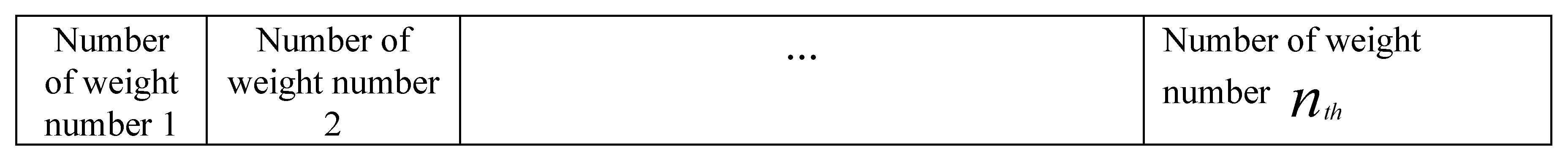
1. A search agent is an array with a specified number of cells, where the number inside each array represents the number of each weight.
Figure 19.
Structure of a search agent.
Stage 2
1. Using the grasshopper and sine cosine algorithms, the best search agent is obtained, which is shown in Figure (21).
2. Each search agent can estimate the weights of the network according to the fitness function. As mentioned, the fitness function is the classification accuracy, which is obtained using Equation (12). As an example, in Figure (20), a neural network with eleven weights (weights between -1 and 1) has been estimated.
Figure 20.
Estimated weights of the neural network.

Figure 21.
Adjustment of random neural network weights pseudo-code.
5. Results of Evaluations
In this section, the software and hardware implementation of the proposed scheme are described in detail. We make a comprehensive evaluation of our proposed scheme in comparison with the new common schemes through simulation. After detailing the simulation settings, protocol comparisons, and metric evaluations, the simulation results are presented along with their analysis.
5.1. Experimental Setup
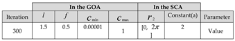
The performance evaluation was conducted using the MATLAB R2021a software. These tests were performed on a 12-core central processing unit with 16 GB of RAM, (ASUS TUF GAMING F15). The settings of the sine cosine optimization and GOA combined Algorithm in Table 3 are specified, with 30 search agents set in 300 iterations. We have four scenarios for simulation. The dataset used is named DS2OS [40], consisting of 256012 samples and 11 features, as indicated in Table 4.
5.2. Metrics for Evaluation
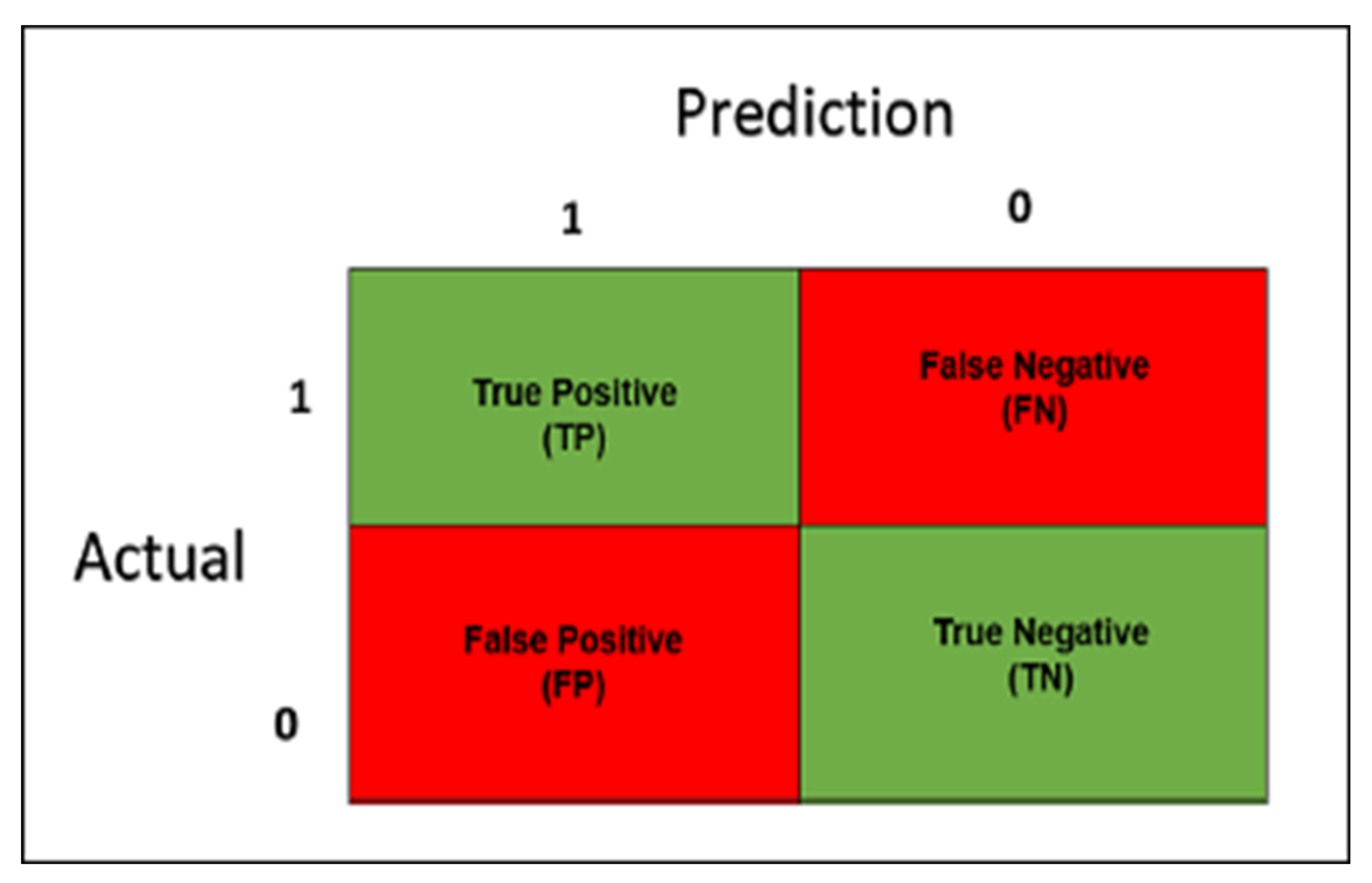
The Confusion Matrix (CM) was used to assess, analyze, and confirm the proposed detection technique. Various factors are taken into account when assessing the proposed model. In the following, performance parameters that are used to evaluate the proposed algorithm are briefly explained. We evaluated the suggested model by considering various performance metrics like accuracy, precision, recall, F1–score, and false alarm rate (FAR). The details of the Confusion matrix are clearly shown in figure 22.
- TN: The number of records whose actual class is negative and the classification algorithm correctly identifies them as negative.
- TP: The number of records whose actual class is positive and the classification algorithm correctly identifies them as positive.
- FP: The number of records whose actual class is negative but the classification algorithm incorrectly identifies them as positive.
- FN: The number of records whose actual class is positive but the classification algorithm incorrectly identifies them as negative.
1. Accuracy
Accuracy is mathematically described as the ratio between accurate positive and negative results to complete the results of the machine learning model.
2. Precision
It is a ratio between truly predicted positive results to true and false-positive results and is mathematically described.
3. Recall (Detection Rate)
It describes the relationship between true positive predictions to true positive and false negative predictions.
4. F1 SCORE
This is a weighted average of precision and recall. The F1 score maintains the balance between precision and recall by considering positive and negative results.
5. False Alarm Rate (FAR)
False alarm rate means the false rate of the detection system. Indeed, malicious behaviors are detected as normal behaviors. Thus, a lower false alarm rate is more desirable.

Table 3.
Settings of the sine cosine optimization and GOA combined algorithm used.
 |
The dataset used is named DS2OS [40], consisting of 256012 samples and 11 features; as indicated in Table 4, apart from this dataset, two other datasets have been used to evaluate the proposed model.
Table 4.
specifications and description of the characteristics of the DS2OS dataset.
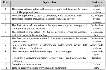 |
The proposed intrusion detection system is based on Random Neural Network (RNN) which learns from observing significant factors in network traffic changes under flood-like attacks in the training samples, labeled as: Source Address, Source Type, Source Location, Destination Address, Destination Type, Destination Location, Access Node Address, Access Node Type, Operation, Data Value, and Transmission Time. The Source and Destination Address refer to the ID of each node, and the Node Type corresponds to the type of equipment, such as whether it is a sensor or an actuator. The operation relates to the number of delivered packets, which can be inspected at the destination node and includes the number of packets delivered from the source node. The input parameter Data Value refers to the numerical value sent in the data, and the packet transmission time is another parameter in the DS2OS dataset. Therefore, 11 effective features for intrusion detection are listed in Table 4. An example of the dataset, transformed into numerical values for use in experiments, is presented in Figure 23.
5.3. Datasets
Due to the constant advancements in network intrusion detection technology, there is now a larger selection of publicly accessible network intrusion detection datasets that are diverse and tailored to specific contexts, serving as valuable resources for research [12]. In addition to the DS2OS dataset [40], two other datasets, CIC-IDS2018 [46] and CIC-IOT2023 [47], were chosen to test the performance of the proposed framework for network intrusion detection in this study. To achieve better detection results, further processing is required. The calculation of the dataset’s imbalance ratio is as follows:
Where is the number of the minority class samples, and denotes the number of the majority class samples.
The CIC-IDS2018 dataset has an imbalance degree of 0.00161 between its smallest and largest classes in the training set, whereas the CIC-IOT2023 dataset has an imbalance degree of 0.00016.
The simulations are reported in four scenarios
- Scenario 1: The results of the proposed model are evaluated using the Support Vector Machine (SVM) method as a parametric method and the K-Nearest Neighbors (KNN) method as a non-parametric method on three datasets.
- Scenario 2: The results of the proposed model are evaluated using the Random Neural Network (RNN) with the specified architecture on three datasets.
- Scenario 3: The results of the improved RNN method are investigated with the Sine cosine optimization and GOA combined algorithm (IOT - RNNEI) on three datasets.
- Scenario 4: The Support Vector Machine (SVM) combined model, K-Nearest Neighbors (KNN) method, and the proposed method in the ensemble learning model are evaluated on three datasets.
Finally, based on the four simulated scenarios and the obtained results, the output of the proposed method (SIRNN-IDS) is compared with other methods. To evaluate the results, metrics such as false alarm rate (FAR), recall (Detection Rate), and accuracy rate are used for comparison.
Scenario 1: Simulation of the Support Vector Machine (SVM) method and K-Nearest Neighbors (KNN) method
Since there are two classes, the number of neighbors in the K-Nearest Neighbors (KNN) method should be odd. For this purpose, different numbers of neighbors including 1, 3, 5, 7, 9 have been tested. In this experiment, a 10-fold cross-validation method has been used for training. The results of the proposed model are only tested with the K-Nearest Neighbors (KNN) method with one neighbor. In these results, the highest accuracy value was 0.966. Additionally, the K-Nearest Neighbors (KNN) method with three neighbors was tested. In these results, the highest accuracy value was 0.964, with the results shown in Table 5. The proposed model results are only tested with the k-Nearest Neighbors (KNN) method with five neighbors.
The results in Table 5 reveal that the highest accuracy value was 0.978. The proposed model's results were also tested using only the K-Nearest Neighbors method with seven neighbors, yielding a maximum accuracy value of 0.965. Also, the proposed model was tested using only the K-Nearest Neighbors method with nine neighbors, achieving a maximum accuracy value of 0.972. As evident from the average accuracy obtained in various settings of this method, the K-Nearest Neighbors method with five neighbors had the best performance with an average accuracy of 0.9732. Figure 24 demonstrates the results with different neighbors.
The results in Figure 24 indicate that the highest classification accuracy value is 0.973. The proposed model's results were also tested using only the K-Nearest Neighbors method with seven neighbors. The performance evaluation of KNN method on CIC-IDS2018 Dataset is outlined in Table 6.
The results in Table 6 show that the highest accuracy value was 0.977. The proposed model's results were also tested using only the K-Nearest Neighbors method with seven neighbors, yielding a maximum accuracy value of 0.966. Further, the proposed model was tested using only the K-Nearest Neighbors method with nine neighbors, achieving a maximum accuracy value of 0.973. As evident from the average accuracy obtained in various settings of this method, the K-Nearest Neighbors method with five neighbors had the best performance with an average accuracy of 0.9731. Figure 25 displays the results with different neighbors.
The results in Figure 25 reveal that the highest classification accuracy value is 0.975. The proposed model's results were also tested using only the K-Nearest Neighbors method with seven neighbors. The performance evaluation of KNN method on CIC-IOT2023 dataset is shown in Table 7.
The results in Table 7 show that the highest accuracy value was 0.978. The proposed model's results were also tested using only the K-Nearest Neighbors method with seven neighbors, yielding a maximum accuracy value of 0.966. Additionally, the proposed model was tested using only the K-Nearest Neighbors method with nine neighbors, achieving a maximum accuracy value of 0.974. As evident from the average accuracy obtained in various settings of this method, the K-Nearest Neighbors method with five neighbors had the best performance with an average accuracy of 0.9724. Figure 26 illustrates the results with different neighbors.
The results in Figure 26 indicate that the highest classification accuracy value is 0.971. The proposed model's results were also tested using only the K-Nearest Neighbors method with seven neighbors. Next, the simulation results with Support Vector Machine (SVM) using different kernels are presented. The proposed model's results were tested using the SVM method with a sigmoid kernel. In these results, the highest accuracy value was 0.984. The proposed model was also tested using only the SVM method with a polynomial kernel, achieving a maximum accuracy value of 0.982. Furthermore, as indicated in Table (8), the proposed model's results were tested using only the SVM method with a Gaussian kernel on DS2OS dataset. In these results, the highest accuracy value was 0.988.
In Table 8, as evident from the average accuracy obtained in various settings of this method, the SVM with a Gaussian kernel had the best performance with an average accuracy of 0.9862, outperforming the k-Nearest Neighbors method in terms of accuracy. Figure 27 illustrates the comparison of results from different settings of the SVM method.
The results of the proposed model were tested using the Support Vector Machine (SVM) method with a sigmoid kernel. In these results, the accuracy value was 0.985. The proposed model was also tested using only the SVM method with a polynomial kernel, achieving an accuracy value of 0.983. Furthermore, as indicated in Figure 27, the proposed model's results were tested using only the SVM method with a Gaussian kernel. In these results, the highest accuracy value was 0.986. Furthermore, as indicated in Table 8, the proposed model's results were tested using only the SVM method with a Gaussian kernel. In these results, the highest accuracy value was 0.988. The performance evaluation of the SVM method on CIC-IDS2018 is shown in Table 9.
According to the average accuracy obtained in various settings of this method in Table 9, the Support Vector Machine with a Gaussian kernel had the best performance with an average accuracy of 0.9847. Table 10 displays the performance evaluation of the SVM method on the CIC-IOT2023 Dataset.
In Table 10, as observed from the average accuracy obtained in various settings of this method, the Support Vector Machine with a Gaussian kernel had the best performance with an average accuracy of 0.9847.
Scenario 2: Simulation of the random neural network method
By analyzing the experiments, the best architecture for the random neural network has been identified. It includes eight hidden layers, with 15 neurons in each layer. table 11 presents the results of the random neural network (RNN) with 10-fold cross-validation on DS2OS dataset.
In Table 11, As evident from the results of ten-fold cross-validation of the Random Neural Network method presented Based on the experiments. the best accuracy result was 0.991, with an average detection accuracy of 0.9901. In Table 12, you can find the performance evaluation of the RNN method on the CIC-IDS2018 dataset.
In Table 12 As evident from the results of ten-fold cross-validation of the Random Neural Network method presented Based on the experiments. the best accuracy result was 0.991, with an average detection accuracy of 0.9895. The performance evaluation of the RNN method on CIC-IOT2023 dataset is reported in Table 13.
In Table 13 As evident from the results of ten-fold cross-validation of the Random Neural Network method presented Based on the experiments. the best accuracy result was 0.993, with an average detection accuracy of 0.9897.
- Scenario S: Simulation of the improved Random Neural Network method with the sine cosine optimization and GOA combined algorithm (IOT - RNNEI)
The experiments have led to the determination of the optimal architecture for the random neural network. This architecture involves eight hidden layers, with 15 neurons in each layer, considering the number of neurons and other neural network settings. table 14 shows the results of the improved random neural network method with the sine cosine and GOA combined algorithm. As evident from the results of ten-fold cross-validation of the proposed method, the best accuracy result was 0.996, with an average detection accuracy of 0.9949.
In Table 14 As evident from the results of ten-fold cross-validation of the Random Neural Network method presented Based on the experiments. the best accuracy result was 0.995, with an average detection accuracy of 0.9949. The performance evaluation of the proposed method on the CIC-IDS2018 dataset is displayed in Table 15.
In Table 15 As evident from the results of ten-fold cross-validation of the Random Neural Network method presented Based on the experiments. the best accuracy result was 0.996, with an average detection accuracy of 0.9944. Table 16 reports the performance evaluation of the proposed method on the CIC-IDS2018 dataset.
In Table 16 As evident from the results of ten-fold cross-validation of the Random Neural Network method presented Based on the experiments. the best accuracy result was 0.996, with an average detection accuracy of 0.9937.
- Scenario 4: Multi-Task Learning Model Simulation
In this section, the best architecture of the tested methods has been experimented in the form of multi-task learning, including the Nearest Neighbor method with five neighbors, Gaussian kernel support vector machine (SVM), and improved random neural network with the sine cosine optimization and GOA algorithm. As outlined in Table 17, the results of the proposed model in multi-task learning show higher accuracy compared to other experiments, with the highest accuracy value being 0.997, though the average is obtained as 0.9956.
The evaluation of the proposed framework, along with other new methods, considered criteria such as recall, false alarm rate, and accuracy rate on three datasets. See Table 18 for the results.
As reported in Table 18, the proposed model is compared with three new methods of 2024 (DL, FL, ET-DCANET). Specifically, Figure 28 shows the difference between various methods with the proposed model on DS2OS based on the recall (detection rate).
Based on the false alarm rate (FAR), Figure 29 demonstrates the variation between different methods and the proposed model on DS2OS.Considering that the lower the FAR, the better the performance of the model.
In Figure 29, the results are shown graphically, the difference between various methods was determined based on the FAR. With the lowest false alarm rate is 0.004. Table 19 shows comparison of various methods and the proposed model on CIC-IDS2018 dataset.
The results in Table 19 show that the highest accuracy value was 99.76%. Figure 30 graphically illustrates the difference between various methods on CIC-IDS2018 dataset based on the recall (detection rate).
Figure 31 graphically shows the difference between various methods on CIC-IDS2018 dataset based on the false alarm rate (FAR).
Figure 31, presenting the results graphically, indicates the difference between various methods with the lowest false alarm rate being 0.003. Table 20 compares various methods and the proposed model on CIC-IOT2023 dataset.
The results in Table 20 show that the highest accuracy value was 99.59%. Figure 32 clearly reveal the comparison between the new methods and the proposed model (IOT - RNNEI) on CIC-IOT2023 dataset in terms of accuracy rate.
Figure 33 graphically indicates the difference between various methods on CIC-IOT2023 dataset based on the recall (detection rate).
Figure 34 graphically displays the difference between various methods on CIC-IOT2023 dataset based on the false alarm rate (FAR).
The accuracy and false alarm rates of current intrusion detection methods can be problematic, which is why we introduced a new model for IOT network intrusion detection to enhance performance. the proposed framework was evaluated on three datasets; as shown in Figure 34 and Figure 35, the proposed model has superior performance on the new dataset (CIC-IOT2023) compared to other methods. Comparison of training time and classification accuracy of RNN and IOT - RNNEI (proposed model) on DS2OS dataset is indicated in Table 21.
As reported in Table 21, in terms of training time, in the standard random neural network, as the number of neurons in the hidden layer increases, so does the execution time due to training via gradient descent. However, in the proposed model, the time spent on training is related to the execution of the sine cosine and GOA combined algorithm. Indeed, Increasing the hidden layer neurons in the neural network expands the dimensions of the sine cosine and GOA combined algorithm, resulting in shorter processing time compared to a random neural network. increasing the number of neurons in the hidden layer of the neural network. it needs to reach the optimal weight values through derivation, and therefore, with an increase in the number of weights, more time is needed for training. In terms of classification accuracy, it is observed that in the standard random neural network, with changes in the number of neurons and hidden layers, the accuracy varies, and even with ten hidden layers with fifteen neurons in each hidden layer, this accuracy does not increase; the best architecture, considering the architecture introduced [6], consists of eight hidden layers with 15 neurons in each hidden layer.
6. Conclusion and Future Works
A proper intrusion detection system's effectiveness depends directly on the choice and effectiveness of the classification method. Tweaking parameters, such as network weights, can enhance a neural network's performance. A method for detecting attacks in IOT networks is outlined in this paper, utilizing evolutionary intelligence and random neural networks. By utilizing a joint algorithm of grasshopper and sine cosine optimization, the proposed model upgraded the architecture and internal parameters of the random neural network. The effectiveness of the proposed model was confirmed on three datasets (DS2OS, CIC-IDS2018, CIC-IOT2023), with an accuracy rate of 99.59%, recall value of 0.9929, and false alarm rate of 0.004. The suggested model was proven to improve data balance and demonstrate outstanding detection performance in network intrusion assignments. However, our suggested model does come with its limitations. We conducted numerous experiments to enhance both the structure and parameters of a neural network for optimal performance. Nevertheless, grasshopper-like evolutionary intelligence algorithms need time to discover the best solution in the search space. The parameters may also need tweaking in various application environments to sustain the model’s peak performance. Moreover, ongoing communication among IOT devices while training the model in the suggested framework could lead to communication overhead. However, our model could save computational resources by utilizing metaheuristic algorithms, although it might require more time for these algorithms to reach the global optimal point, particularly with extensive IOT datasets. If the IOT devices lack computational power, the algorithm training time could go up. The grasshopper optimization algorithm can only tackle single-objective problems involving continuous variables. Furthermore, the proposed framework demands consistent communication between IOT devices while training the model, leading to potential communication overhead. The data gathered from various devices is recognized to display diverse quality characteristics. Achieving generalizability of the model in diverse IOT datasets is a difficult task. The deployment of the suggested model in the live test environment is uncertain. Future work will focus on optimizing the model with various metaheuristic optimization algorithms in vehicular networks.
Declarations
- *Funding: No funding was received.
- *Conflicts of interest/Competing interests: There is no conflict of interest.
- *Availability of data and material: 'Not applicable'.
- *Authors' contributions: All authors contributed equally to this manuscript.
- *Acknowledgements: 'Not applicable'.
- *Consent to participate: 'Not applicable'.
- *Consent for publication: 'Not applicable'.
- *Ethics approval: The paper is original, and any other publishing house is not considering it for publication. The paper reflects the author's own research and analysis in a truthful and complete manner. All sources used are properly disclosed (correct citation).
References
- Chao Chen, Li-Chun Wang, CHIH-Min Yu, (2022), “D2CRP: A Novel Distributed 2-Hop Cluster Routing Protocol for Wireless Sensor Networks” IEEE INTERNET OF THINGS JOURNAL. [CrossRef]
- LALIT Kumar, Pradeep Kumar, (2022), “BITA-Based Secure and Energy-Efficient Multi-Hop Routing in IOT-WSN” CYBERNETICS AND SYSTEMS. [CrossRef]
- SANGREZ Khan a, Ahmad NASEEM ALVI a, Muhammad AWAIS JAVED, Yasser D. Al-OTAIBI, Ali KASHIF Bashir, (2021), “An efficient medium access control protocol for RF energy harvesting based IOT devices” Computer Communications. [CrossRef]
- MAHAMAT M, JABER G, BOUABDALLAH A, (2023), “Achieving efficient energy-aware security in IOT networks: a survey of recent solutions and research challenges” Wireless Networks. [CrossRef]
- PARISA RAHMANI, MOHAMAD AREFI, (2023), “Improvement of energy-efficient resources for cognitive internet of things using learning automata” Peer-to-Peer Networking and Applications. [CrossRef]
- SHAHID LATIF, ZHUO ZOU, ZEBA IDREES, JAWAD AHMAD, (2020), “Novel Attack Detection Scheme for the Industrial Internet of Things using a Lightweight Random Neural Network” IEEE Access Digital Object Identifier. [CrossRef]
- ZHENDONG Wang, Xin Yang, ZHIYUAN Zeng, DAOJING He, Sammy Chan, (2024), “A hierarchical hybrid intrusion detection model for industrial internet of things” Peer-to-Peer Networking and Applications. [CrossRef]
- N Singh, A DUMKA, R Sharma, (2020), “Comparative Analysis of Various Techniques of DDOS Attacks for Detection & Prevention and Their Impact in MANET”, Performance Management of Integrated Systems and its Applications in Software Engineering. [CrossRef]
- H Liu, D Chen, (2021), “Wind Power Short-Term Forecasting Based on LSTM Neural Network with Cuckoo Algorithm”, Journal of Physics: Conference Series. [CrossRef]
- SHAHRZAD SAREMI, SEYEDALI MIRJALILI, Andrew Lewis, (2017), “Grasshopper Optimization Algorithm: Theory and application” Advances in Engineering Software. [CrossRef]
- MIRJALILI, S. (2016). “SCA: A Sine Cosine Algorithm for solving optimization problems” Knowledge-Based Systems. [CrossRef]
- Xiao Wang, Lie Dai, GUANG Yang, (2024), “A network intrusion detection system based on deep learning in the IOT” The Journal of Supercomputing. [CrossRef]
- CHONGZHOU ZHONG, ARINDAM SARKAR, SARBAJIT MANNA, Mohammad ZUBAIR Khan, ABDULFATTAH NOORWALI, Ashish Das, KOYEL Chakraborty, (2024), “Federated learning-guided intrusion detection and neural key exchange for safeguarding patient data on the internet of medical things” International Journal of Machine Learning and Cybernetics. [CrossRef]
- ANUVELAVAN SUBRAMANIAM, SURESHKUMAR CHELLADURAI, Stanly Kumar ANDE, SATHIYANDRAKUMAR Srinivasan, (2024), “Securing IOT network with hybrid evolutionary lion intrusion detection system: a composite motion optimization algorithm for feature selection and ensemble classification” JOURNAL OF EXPERIMENTAL & THEORETICAL ARTIFICIAL INTELLIGENCE. [CrossRef]
- G. SATHISH Kumar, K. G. SATHISH Kumar, K. PREMALATHA, G. Uma MAHESHWARI, P. Rajesh KANNA, G. VIJAYA, M. NIYAASHINI, (2024), “Differential privacy scheme using Laplace mechanism and statistical method computation in deep neural network for privacy preservation” Engineering Applications of Artificial Intelligence. [CrossRef]
- T.M. NITHYA, P. T.M. NITHYA, P. DHIVYA, S.N. SANGEETHAA, P. Rajesh KANNA, (2024), “TB-MFCC MULTIFUSE feature for emergency vehicle sound classification using MULTISTACKED CNN – Attention BILSTM” Biomedical Signal Processing and Control. [CrossRef]
- G. SATHISH Kumar, K. G. SATHISH Kumar, K. PREMALATHA, G. Uma MAHESHWARI, P. Rajesh KANNA. (2023), “No more privacy Concern: A privacy-chain based homomorphic encryption scheme and statistical method for privacy preservation of user’s private and sensitive data” Expert Systems with Applications. [CrossRef]
- KARTHIKA S, T Priyanka, J. INDIRAPRIVADHARSHINI, DR S SADESH, RAJESHKUMAR G, Rajesh KANNA P, (2023), “Prediction of Weather Forecasting with Long Short-Term Memory using Deep Learning” Proceedings of the Fourth International Conference on Smart Electronics and Communication (ICOSEC). [CrossRef]
- T.M. NITHYA, P. T.M. NITHYA, P. Rajesh KANNA, S. VANITHAMANI, P. SANTHI, (2023), “An Efficient PM - Multisampling Image Filtering with Enhanced CNN Architecture for Pneumonia Classification” Biomedical Signal Processing and Control. [CrossRef]
- E. MYTHILI, DR.S. E. MYTHILI, DR.S. VANITHAMANI, DR Rajesh KANNA, DR RAJESHKUMAR G, K GAYATHRI, R. HARSHA, (2023), “AMLPDS: An Automatic Multi-Regional License Plate Detection System based on EASYOCR and CNN Algorithm” Proceedings of the Second International Conference on Edge Computing and Applications (ICECAA 2023). [CrossRef]
- P. DHIVYA, P. P. DHIVYA, P. Rajesh KANNA, K. DEEPA, S. SANTHIYA, (2023), “Square Static – Deep Hyper Optimization and Genetic Meta-Learning Approach for Disease Classification” IETE JOURNAL OF RESEARCH. [CrossRef]
- P. Rajesh KANNA, G. P. Rajesh KANNA, G. RAJESHKUMAR, S. SRIRAM, S. SADESH, C. VINU, LOGANATHAN Mani, (2023), “Effective Scheduling of Real-Time Task in Virtual Cloud Environment Using Adaptive Job Scoring Algorithm” Proceedings of International Conference on Advanced Communications and Machine Intelligence, Studies in Autonomic, Data-driven and Industrial Computing. [CrossRef]
- A. PANDIARAJ, S. Lakshmana Prakash, R. Gopal, P. Rajesh KANNA, (2022), “Generating Art and Music Using Deep Neural Networks” Artificial Intelligent Techniques for Wireless Communication and Networking. [CrossRef]
- P. Rajesh KANNA, P. SANTHI, (2022), “Hybrid Intrusion Detection using Map Reduce based Black Widow.
- Optimized Convolutional Long Short-Term Memory Neural Networks” Expert Systems with Applications. [CrossRef]
- P Rajesh KANNA, P SANTHI, (2021), “Unified Deep Learning approach for Efficient Intrusion Detection System using Integrated Spatial–Temporal Features” Knowledge-Based Systems. [CrossRef]
- P. RAJESH KANNA, K. SINDHANAISELVAN, M.K. VIJAYMEENA, (2017), “A Defensive Mechanism based on PCA to Defend Denial-of-Service Attack” International Journal of Security and Its Application. [CrossRef]
- DR GAYATHIRI B, BRINDHA P, KARTHIKA I, SARANYAE, DR RAJESHKUMAR G, DR Rajesh KANNA P, (2023), “Machine Learning based Crop Suitability Prediction and FERTILISER Recommendation System” Proceedings of the Fourth International Conference on Electronics and Sustainable Communication Systems. [CrossRef]
- HARSHA R, KARTHIKA S, MOHANA PRIYA D, DR Rajesh KANNAP, DR RAJESHKUMAR G, MYTHILIE, (2023), “FOLLA Disease Detection using In-Depth Learning” Proceedings of the Second International Conference on Applied Artificial Intelligence and Computing. [CrossRef]
- SRIRAM S, S SANTHIYA, RAJESHKUMAR G, S. GAYATHRI, K. VIJAYA, Rajesh KANNA P, (2023), “Predict the Quality of Freshwater using Support Vector Machines” Proceedings of the Second International Conference on Applied Artificial Intelligence and Computing. [CrossRef]
- Ravi SHEKHAR Tiwari, D. Lakshmi, TAPAN Kumar Das, ASIS Kumar TRIPATHY, KUAN-CHING Li, (2024), “A lightweight optimized intrusion detection system using machine learning for edge-based IIOT security” Telecommunication Systems. [CrossRef]
- P.RAJESH KANNA, R.VIKRAM, (2020), “AAgricultural Robot – A pesticide spraying device”A International Journal of Future Generation Communication and Networking, https://www.researchgate.net/publication/340827655.
- PA.PANDIARAJ, Dr. S. Lakshmana Prakash, P. Rajesh KANNA, (2021), “EFFECTIVE HEART DISEASE PREDICTION USING HYBRIDMACHINE LEARNING” Proceedings of the Third International Conference on Intelligent Communication Technologies and Virtual Mobile Networks. [CrossRef]
- ANITTHA GOVINDARAM, JEGATHEESAN A, (2024), “FLBC-IDS: a federated learning and BLOCKCHAIN-based intrusion detection system for secure IOT environments” Multimedia Tools and Applications. [CrossRef]
- NANNAN XIE, CHUANXUE Zhang, QIZHAO Yuan, Jing Kong, XIAOQIANG Di, (2024), “IOV-BCFL: An intrusion detection method for IOV based on BLOCKCHAIN and federated learning” Ad Hoc Networks. [CrossRef]
- Ameer El-Sayed, WAEL Said, Amr TOLBA, Yasser ALGINAHI, Ahmed A. TOONY, (2024), “MP-GUARD: A novel multi-pronged intrusion detection and mitigation framework for scalable SD-IOT networks using cooperative monitoring, ensemble learning, and new P4-extracted feature set” Computers and Electrical Engineering. [CrossRef]
- L. MADHURIDEVI, N. V. S. SREE RATHNA Lakshmi, (2024), “Metaheuristic assisted hybrid deep classifiers for intrusion detection: a big data perspective” Wireless Networks. [CrossRef]
- PEIFENG Liang, Lina Yang, ZENGGANG, XIONG, XUEMIN Zhang, Gang Liu, (2024), “Multilevel Intrusion Detection Based on Transformer and Wavelet Transform for IOT Data Security” IEEE INTERNET OF THINGS JOURNAL. [CrossRef]
- SAYEDA SUAIBA Anwar, ASADUZZMAN, Iqbal H. SARKER, (2024), “A differential privacy aided DEEPFED intrusion detection system for IOT applications” Security Privacy. [CrossRef]
- Samira RAJABI, SAMANE ASGARI, SHAHRAM JAMALI, Reza FOTOHI, (2024), “An Intrusion Detection System Using the Artificial Neural Network-based Approach and Firefly Algorithm” Wireless Personal Communications. [CrossRef]
- M.-O. PAHL and F.-X. AUBET, (2018), “Ds2Os Traffic Traces IOT Traffic Traces Gathered in a The Ds2Os IOT Environment” [Online]. Available: https://www.kaggle.com/francoisxa/ds2ostraffictraces.
- M. Hasan, M. M. Islam, M. I. I. ZARIF, M. M. A. Hashem, (2019), “Attack and anomaly detection in IOT sensors in IOT sites using machine learning approaches” Internet Things.
- MURUGAN Ramachandran, SEYEDALI MIRJALILI, MORTEZA NAZARI-HERIS, DEIVA SUNDARI PARVATHYSANKAR, ARUNACHALAM SUNDARAM, CHRISTOBER ASIR RAJAN Charles GNANAKKAN, (2022), “A hybrid Grasshopper Optimization Algorithm and Harris Hawks Optimizer for Combined Heat and Power Economic Dispatch problem” Engineering Applications of Artificial Intelligence. [CrossRef]
- ARPITA Srivastava, DITIPRIVA Sinha, (2024), “PSO-ACO-based bi-phase lightweight intrusion detection system combined with GA optimized ensemble classifiers” Cluster Computing. [CrossRef]
- MADINI O, ALASSAFI, (2024), “Securing IIOT operations with recurrent federated network-based enhanced local search grasshopper” Neural Computing and Applications. [CrossRef]
- R. Alexander, K. Pradeep Mohan Kumar, (2024), “FWICSS‑Federated Watermarked Ideal Client Selection Strategy for Internet of Things (IOT) Intrusion Detection System” Wireless Personal Communications. [CrossRef]
- SHARAFALDIN. I, HABIBI LASHKARI. A, GHORBANI. AA (2018) “Toward generating a new intrusion detection dataset and intrusion traffic characterization” In: Proceedings of the 4th International Conference on Information Systems Security and Privacy - ICISSP, INSTICC SCITE Press, pp 108–116. [CrossRef]
- NETO ECP, DADKHAH S, Ferreira R et al (2023) CICIOT 2023: “a real-time dataset and benchmark for large-scale attacks in IOT environment” Sensors. [CrossRef]
Figure 3.
Impact of parameters [10].
Figure 3.
Impact of parameters [10].
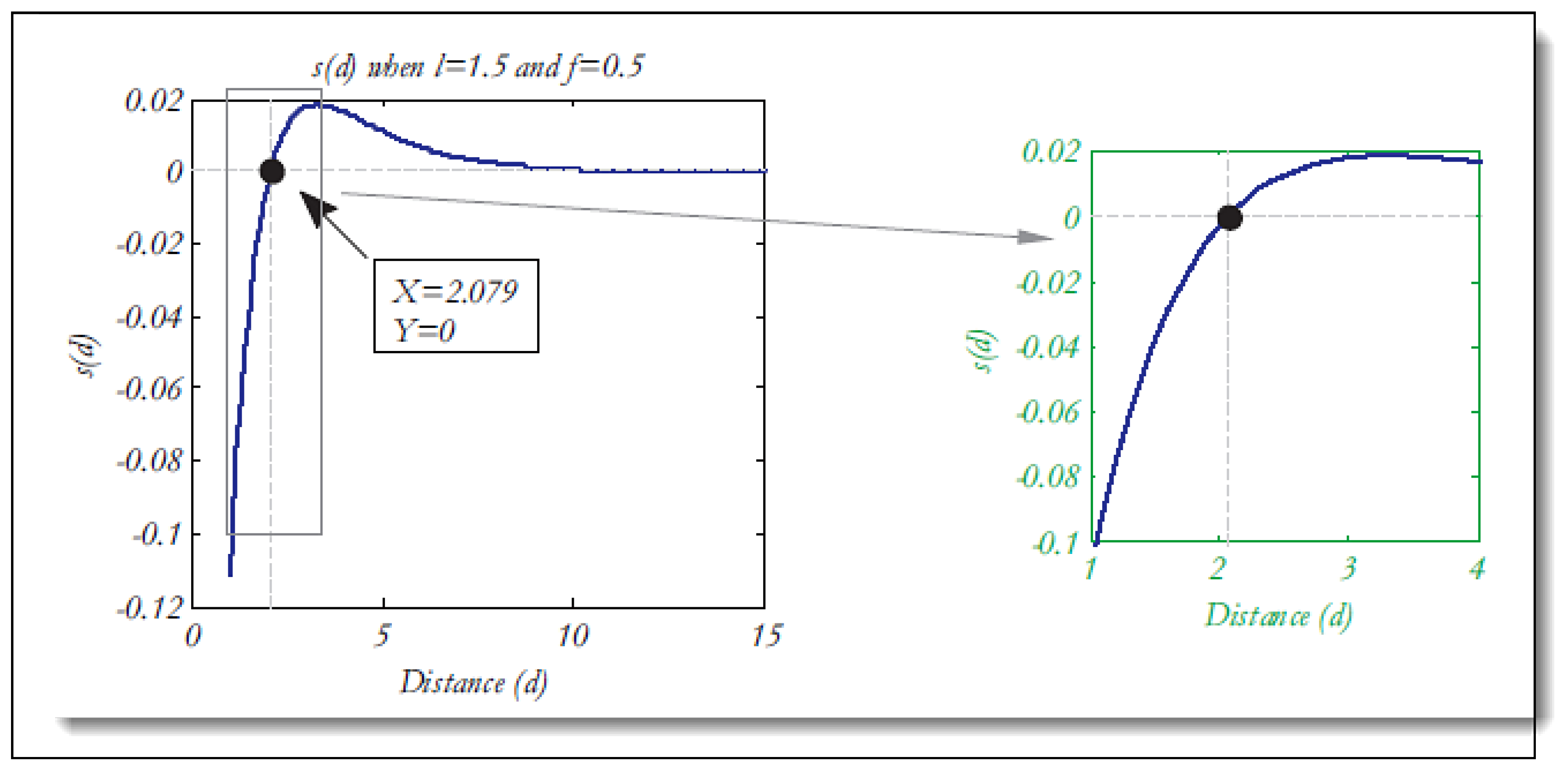
Figure 4.
Influence of parameters (intensity of attraction) and (attraction scale length) on generating various movements [10].
Figure 4.
Influence of parameters (intensity of attraction) and (attraction scale length) on generating various movements [10].
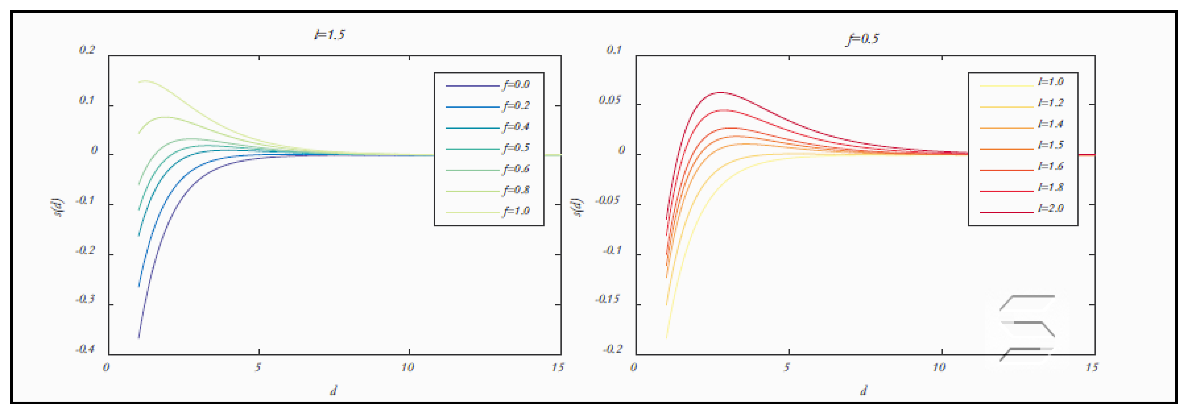
Figure 5.
Conceptual model of interactions between grasshoppers and comfort zone [10].
Figure 5.
Conceptual model of interactions between grasshoppers and comfort zone [10].
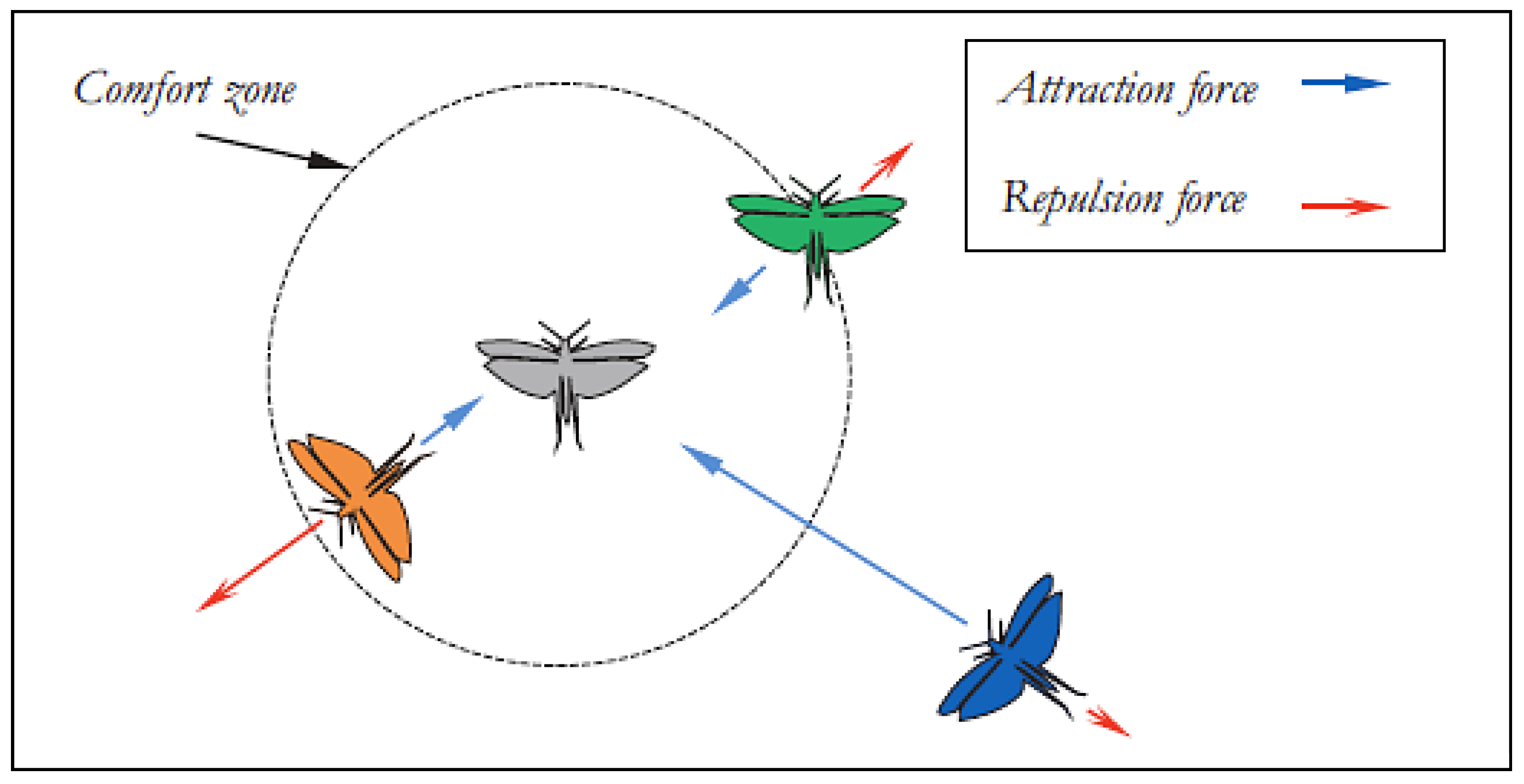
Figure 6.
Behavior of grasshoppers in 2D Space [10].
Figure 6.
Behavior of grasshoppers in 2D Space [10].
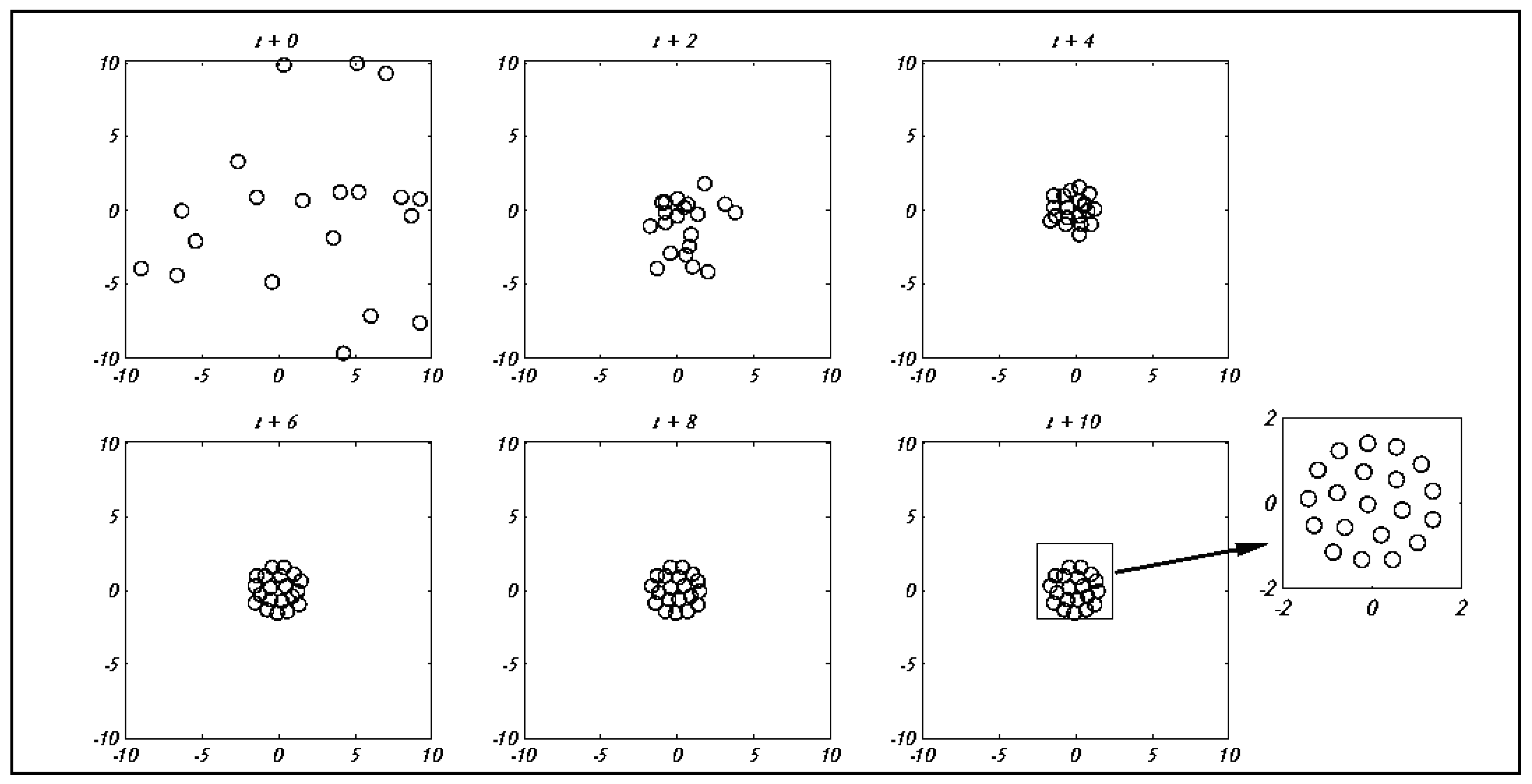
Figure 7.
Impact of parameter C on the movement and convergence of grasshoppers to the global optimum [10].
Figure 7.
Impact of parameter C on the movement and convergence of grasshoppers to the global optimum [10].

Figure 8.
Pseudo codes of the GOA algorithm [10].
Figure 8.
Pseudo codes of the GOA algorithm [10].
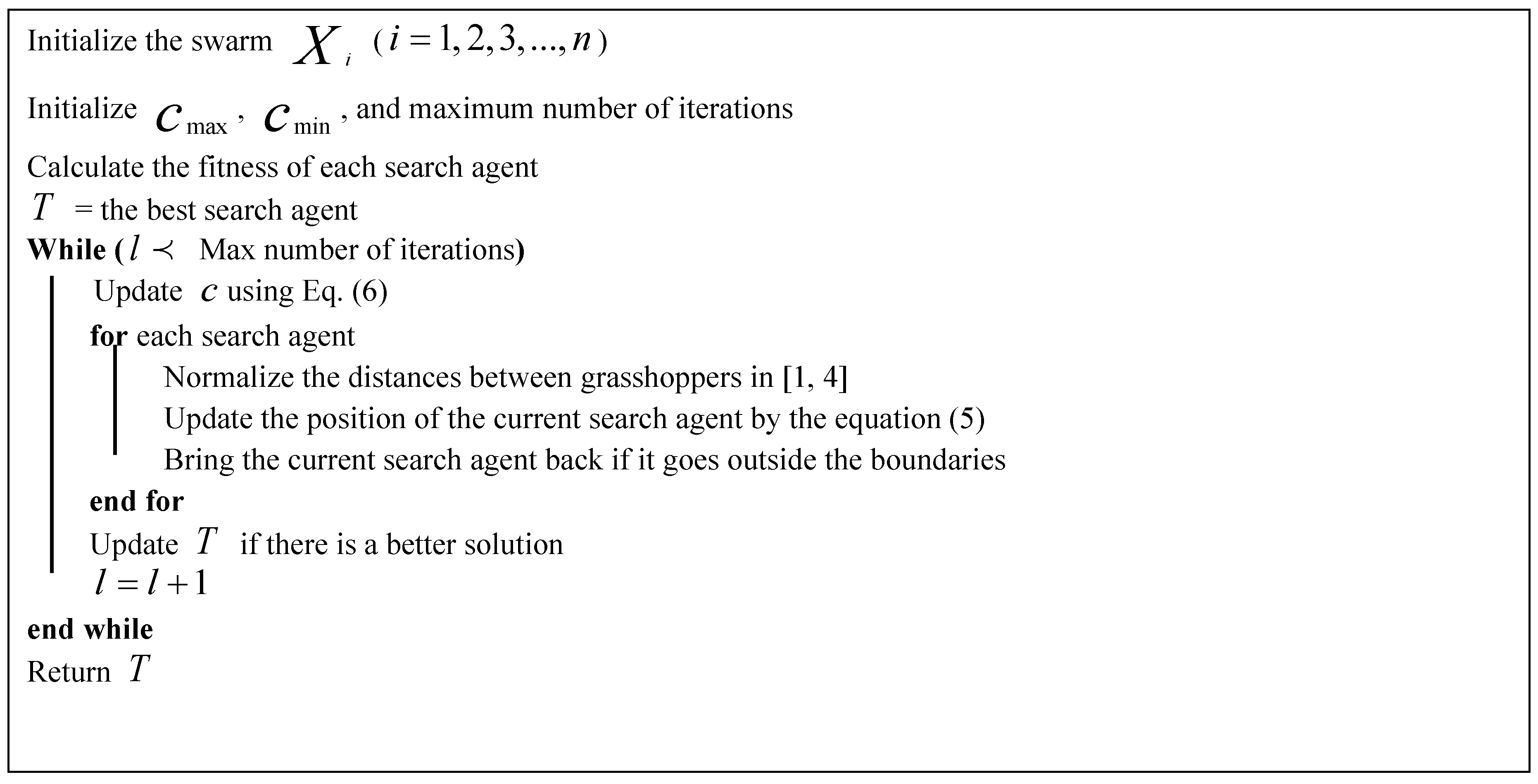
Figure 9.
Impact of parameter on wave movement in the sine cosine optimization algorithm [11].
Figure 9.
Impact of parameter on wave movement in the sine cosine optimization algorithm [11].
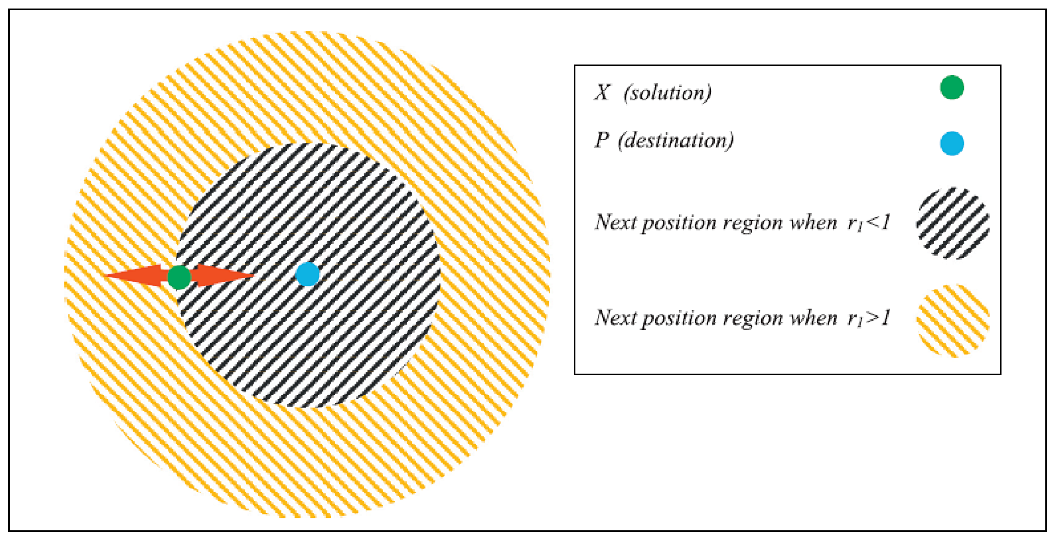
Figure 10.
Impact of parameter on exploration and exploitation in the sine cosine optimization algorithm [11].
Figure 10.
Impact of parameter on exploration and exploitation in the sine cosine optimization algorithm [11].
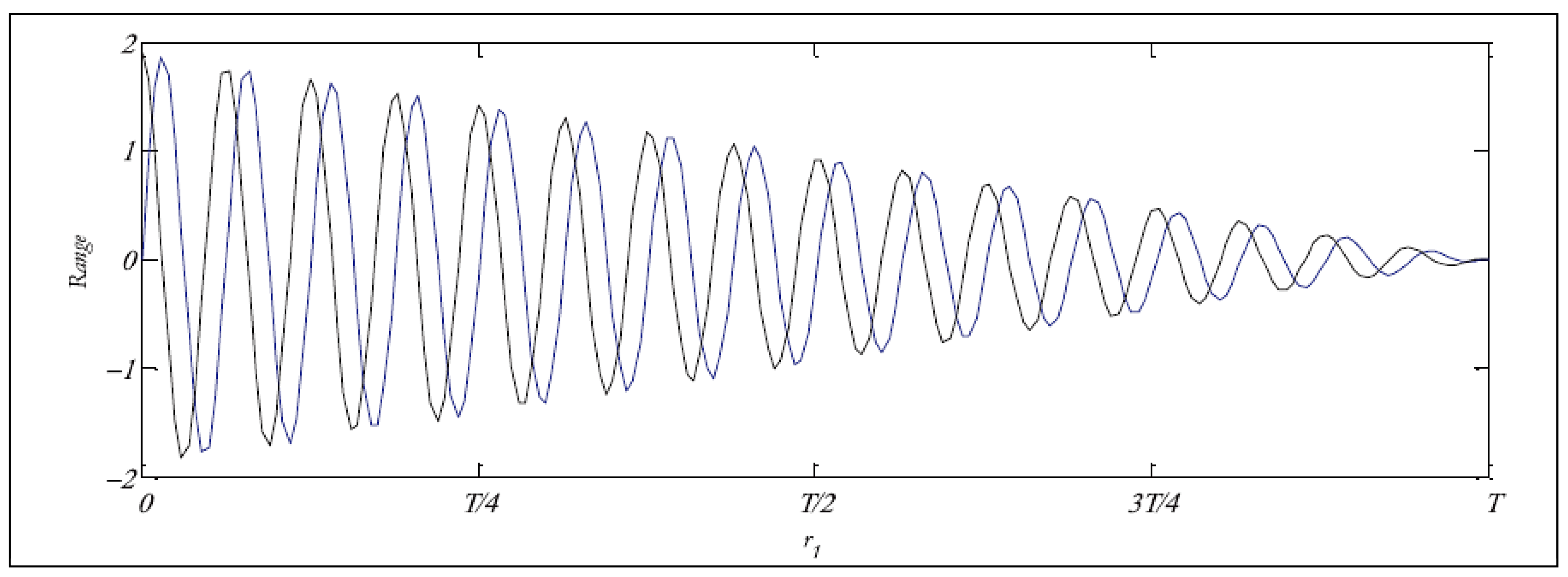
Figure 11.
Impact of parameter on wave movement in the sine cosine optimization algorithm [11].
Figure 11.
Impact of parameter on wave movement in the sine cosine optimization algorithm [11].
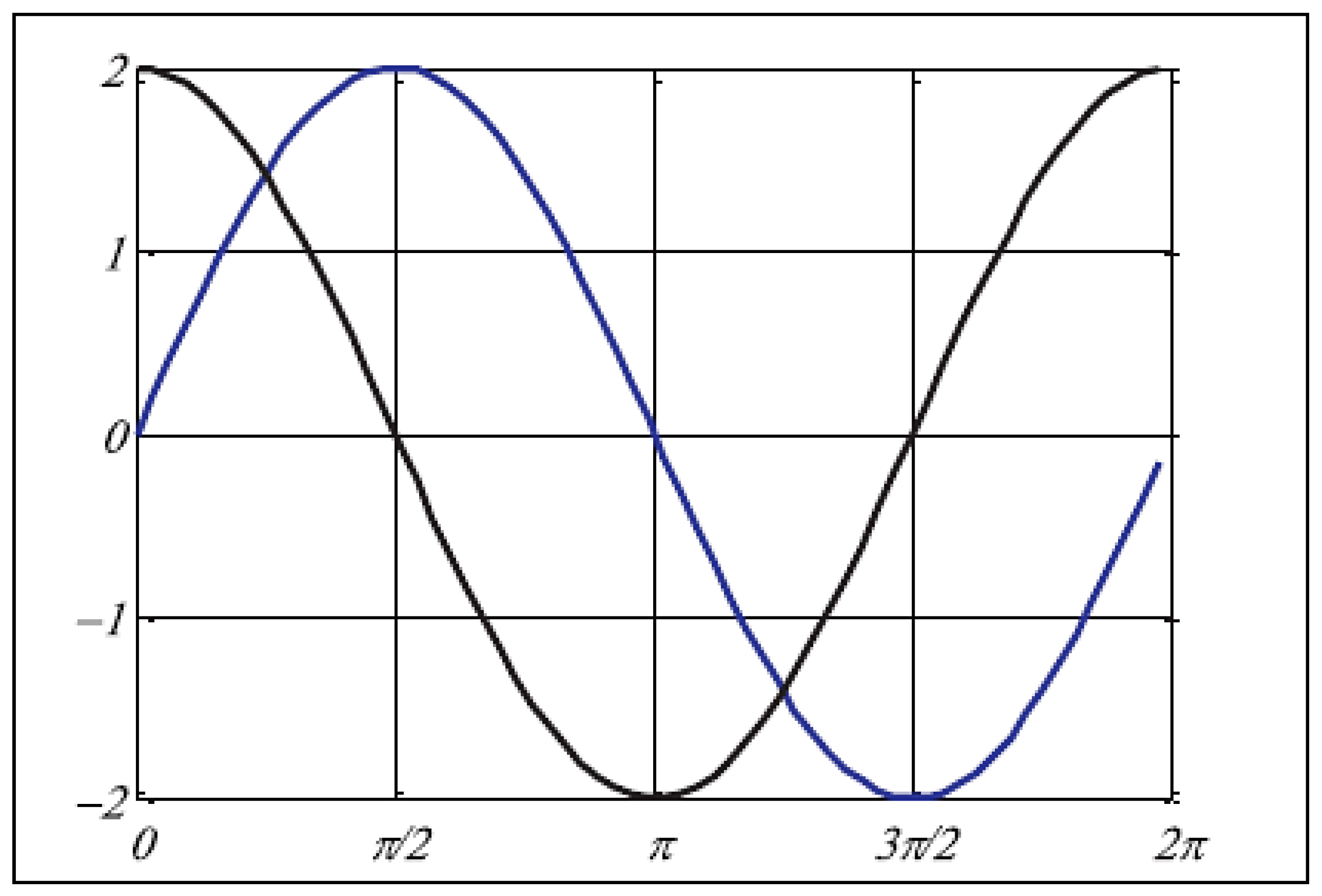
Figure 12.
Pseudo codes of the sine cosine algorithm [11].
Figure 12.
Pseudo codes of the sine cosine algorithm [11].
Figure 23.
Representation of the eleven DS2OS dataset features [6].
Figure 23.
Representation of the eleven DS2OS dataset features [6].

Figure 24.
Comparison of different results in the K-Nearest Neighbors method on DS2OS dataset.
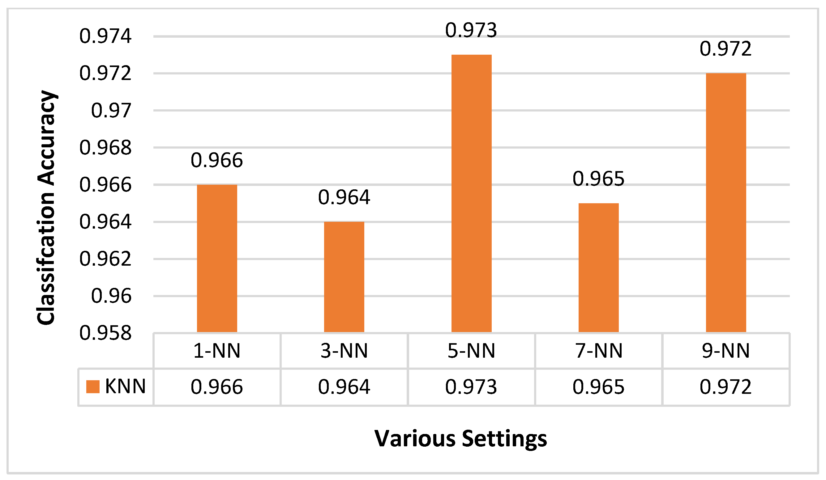
Figure 25.
Comparison of different results in the K-Nearest Neighbors method on CIC-IDS2018 dataset.
Figure 25.
Comparison of different results in the K-Nearest Neighbors method on CIC-IDS2018 dataset.
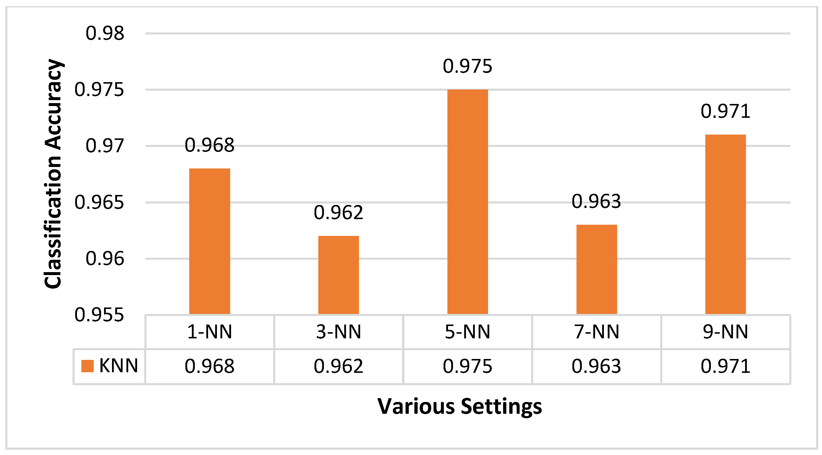
Figure 26.
Comparison of different results in the K-Nearest Neighbors method on CIC-IOT2023 dataset.
Figure 26.
Comparison of different results in the K-Nearest Neighbors method on CIC-IOT2023 dataset.
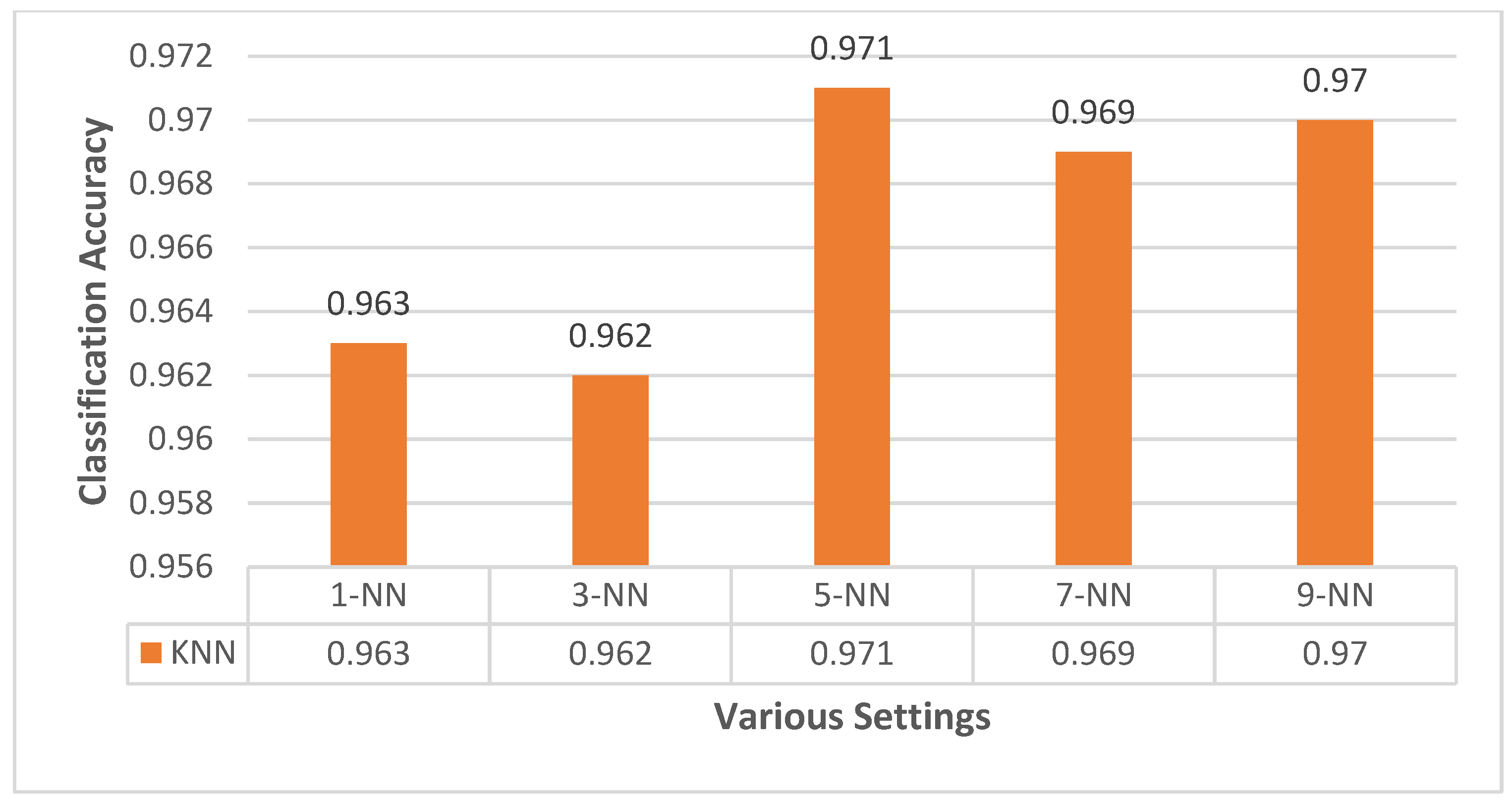
Figure 27.
Comparison of different results in support vector machine on DS2OS dataset.
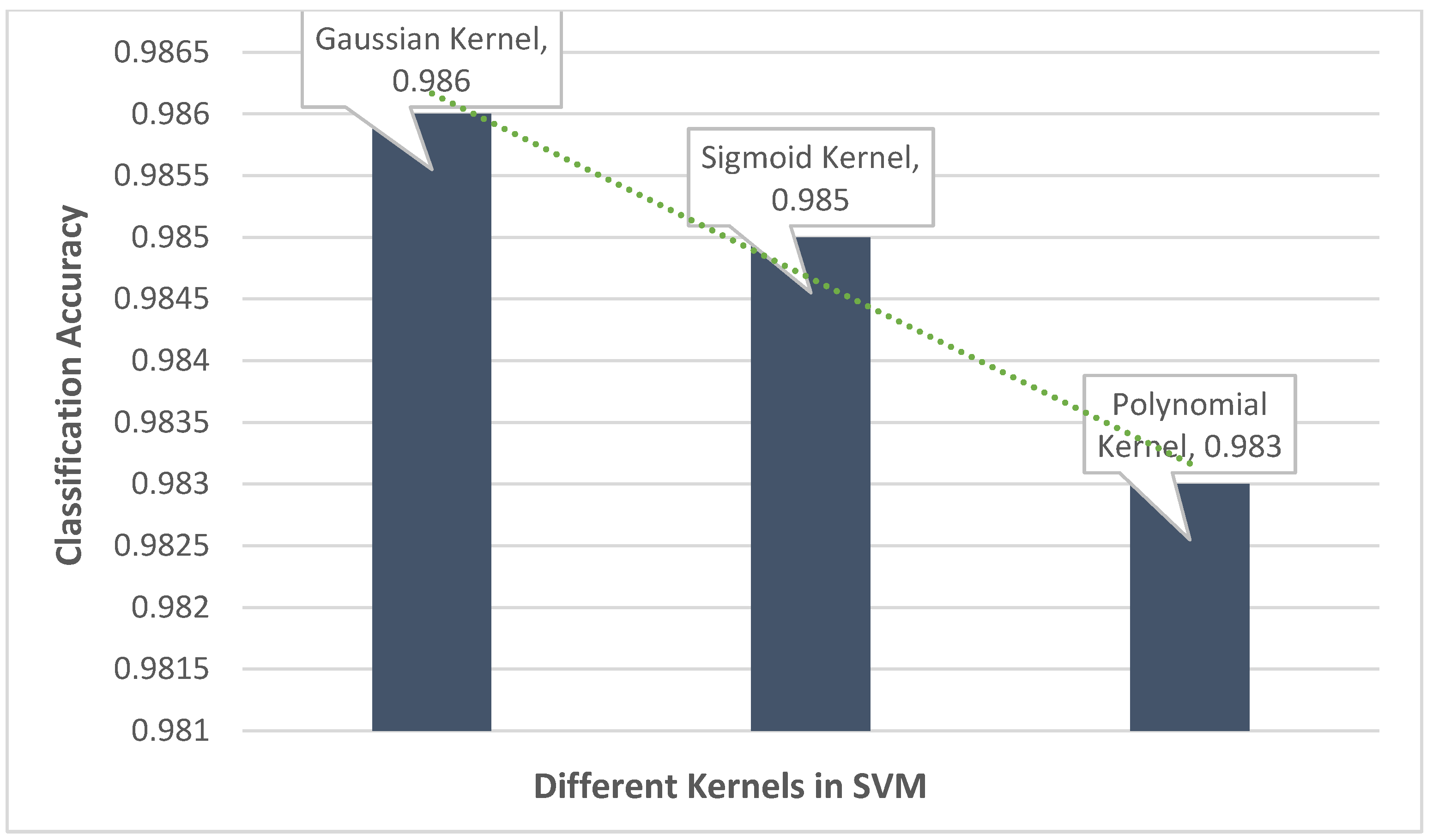
Figure 28.
Comparison of the tested methods and the proposed model on DS2OS dataset.
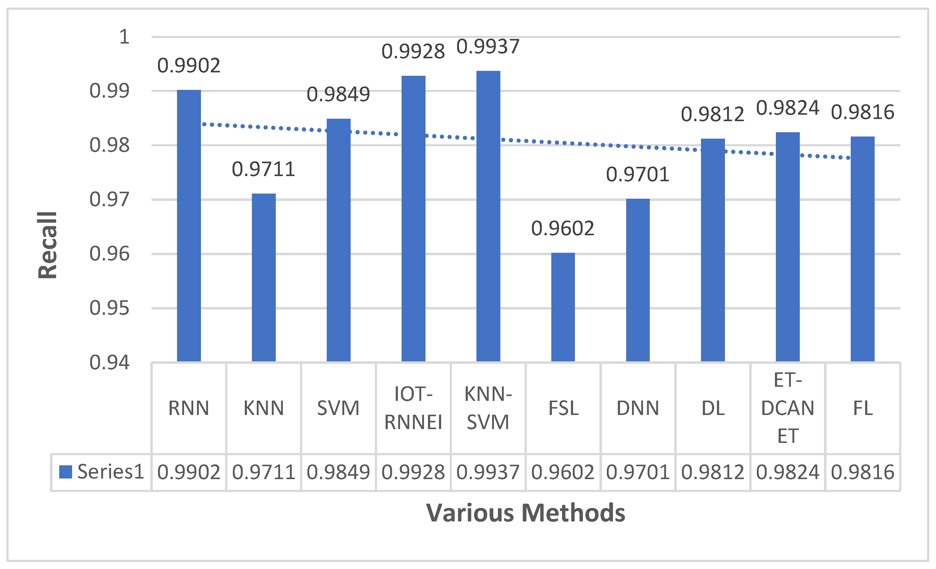
Figure 29.
Comparison of the tested methods and the proposed model on DS2OS dataset.
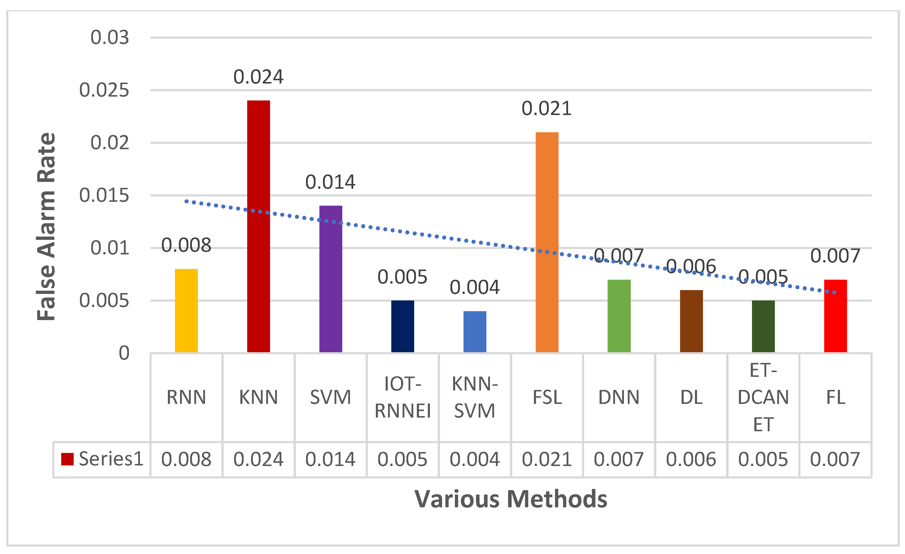
Figure 30.
Comparison of the Tested Methods and the Proposed Model on CIC-IDS2018 Dataset.
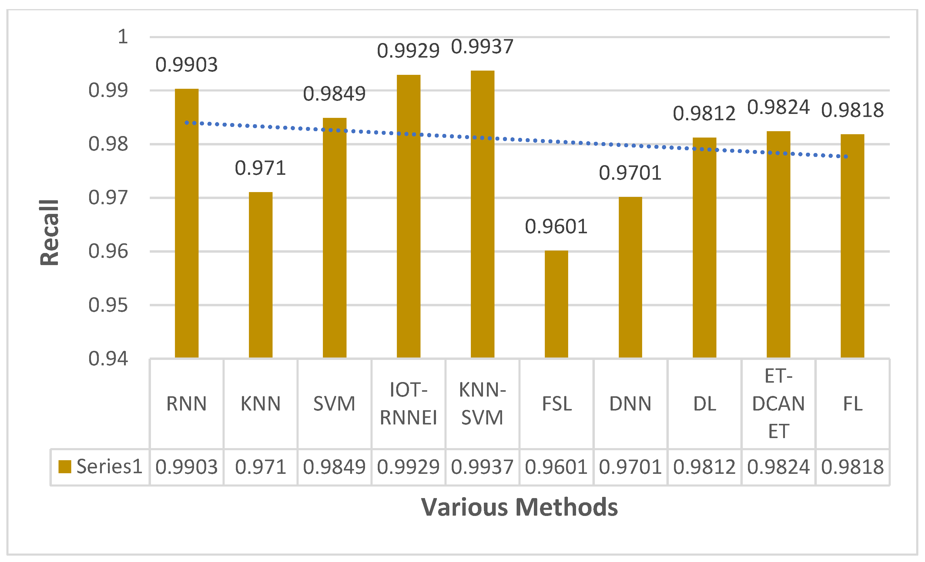
Figure 31.
Comparison of the tested methods and the proposed model on CIC-IDS2018 dataset.
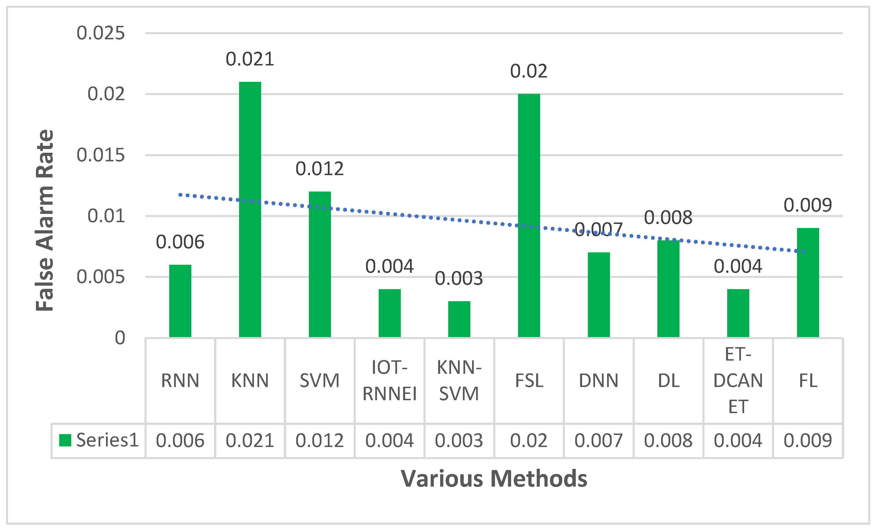
Figure 32.
Comparison of the tested methods and the proposed model on CIC-IOT2023 dataset.
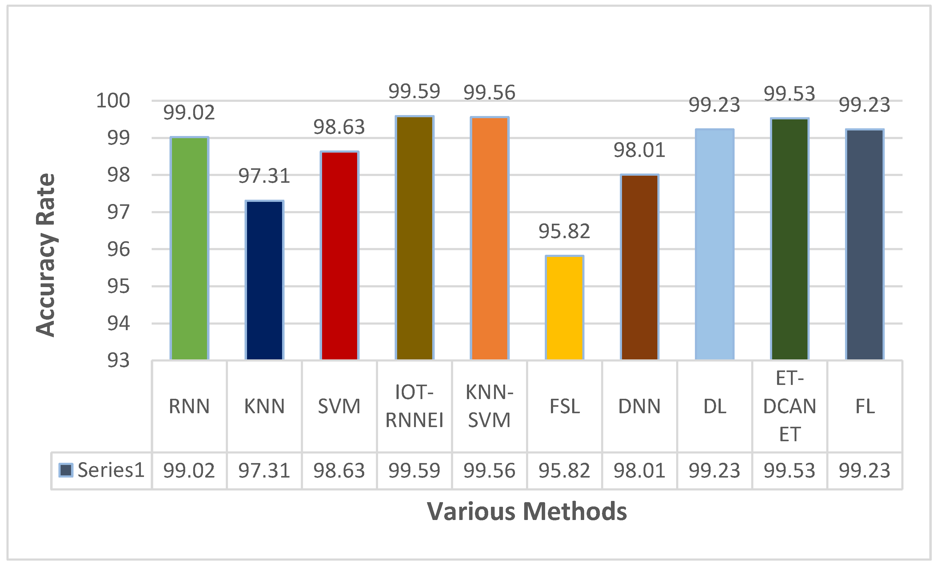
Figure 33.
Comparison of the tested methods and the proposed model on CIC-IOT2023 dataset.
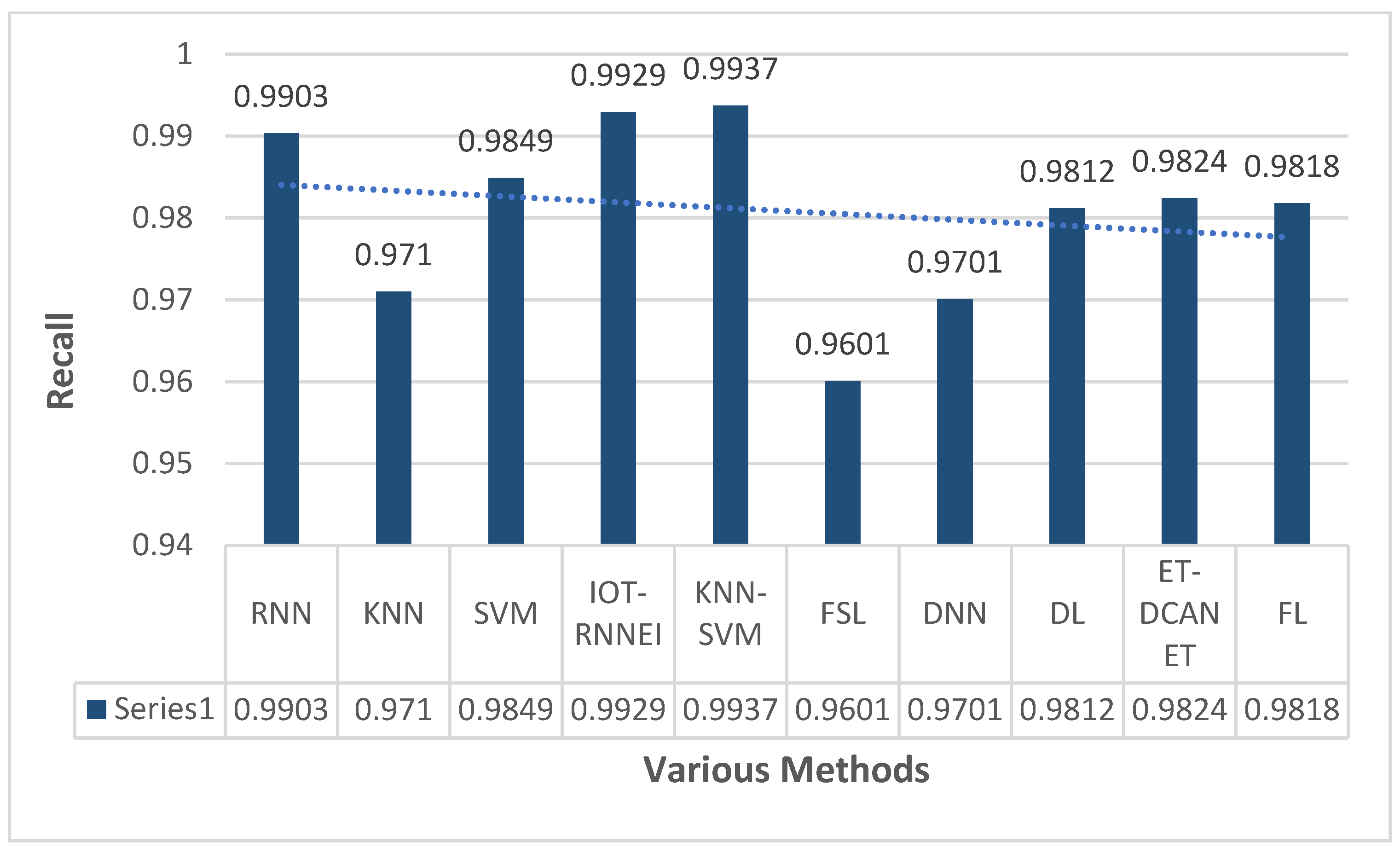
Figure 34.
Comparison of the tested methods and the proposed model on CIC-IOT2023 dataset.
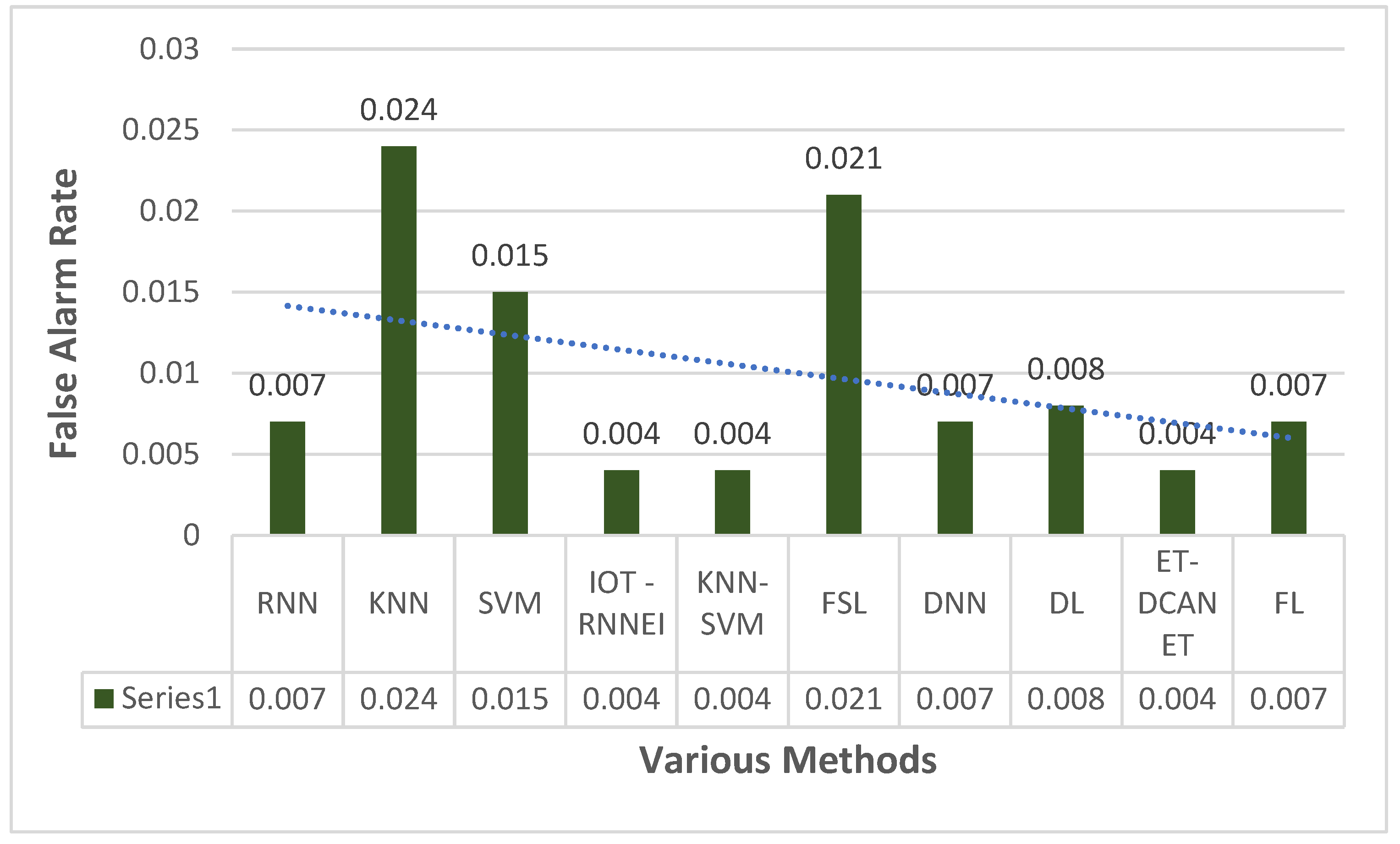
Table 1.
Evaluating the different methods used to analyze the research gap.
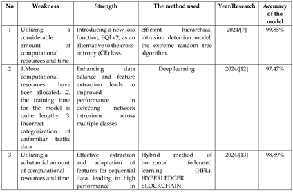 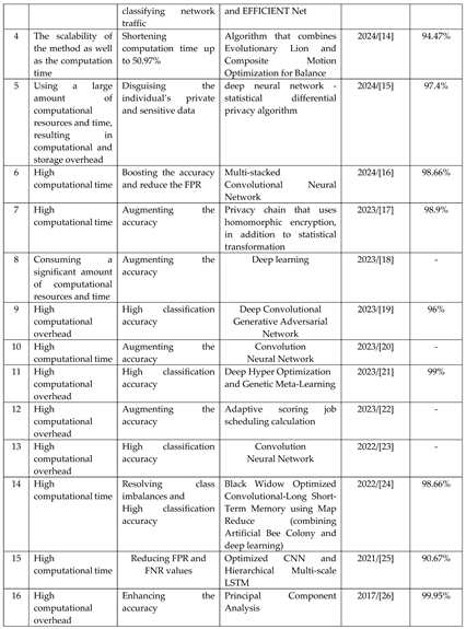 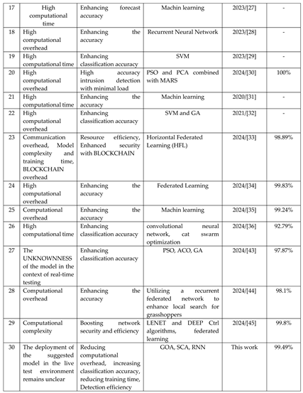
|
Table 2.
Breakdown of the assaults in the DS2OS dataset.
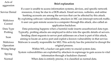 |
Table 5.
Performance evaluation of KNN method with 5 neighbors on DS2OS dataset.
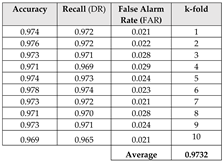 |
Table 6.
Performance evaluation of KNN method with 5 neighbors on CIC-IDS2018 dataset.
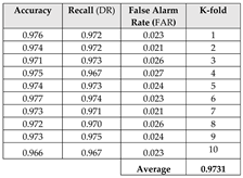 |
Table 7.
Performance evaluation of KNN method with 5 neighbors on CIC-IOT2023 dataset.
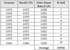 |
Table 8.
Performance evaluation of the SVM method with a Gaussian Kernel on DS2OS dataset.
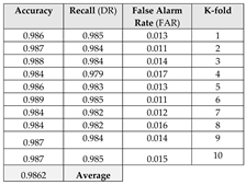 |
Table 9.
Performance evaluation of the SVM method with a Gaussian kernel on CIC-IDS2018 dataset.
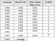 |
Table 10.
Performance evaluation of the SVM method with a Gaussian kernel on CIC-IOT2023 dataset.
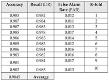 |
Table 11.
The DS2OS dataset was used to evaluate the performance of the RNN method with eight hidden layers and 15 neurons in each layer.
Table 11.
The DS2OS dataset was used to evaluate the performance of the RNN method with eight hidden layers and 15 neurons in each layer.
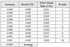 |
Table 12.
Performance evaluation of the RNN method with eight hidden layers and 15 neurons in each layer on CIC-IDS2018 dataset.
Table 12.
Performance evaluation of the RNN method with eight hidden layers and 15 neurons in each layer on CIC-IDS2018 dataset.
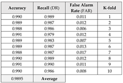 |
Table 13.
The RNN method with eight hidden layers and fifteen neurons in each layer was evaluated on the CIC-IOT2023 dataset.
Table 13.
The RNN method with eight hidden layers and fifteen neurons in each layer was evaluated on the CIC-IOT2023 dataset.
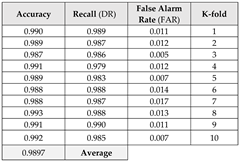 |
Table 14.
Performance evaluation of the proposed method (IOT - RNNEI) with eight hidden layers and 15 neurons in each layer on DS2OS dataset.
Table 14.
Performance evaluation of the proposed method (IOT - RNNEI) with eight hidden layers and 15 neurons in each layer on DS2OS dataset.
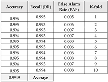 |
Table 15.
Evaluating the proposed method (IOT - RNNEI) with 8 hidden layers and 15 neurons per layer on the CIC-IDS2018 dataset.
Table 15.
Evaluating the proposed method (IOT - RNNEI) with 8 hidden layers and 15 neurons per layer on the CIC-IDS2018 dataset.
 |
Table 16.
Performance evaluation of the proposed method (IOT - RNNEI) with eight hidden layers and 15 neurons in each layer on CIC-IOT2023 dataset.
Table 16.
Performance evaluation of the proposed method (IOT - RNNEI) with eight hidden layers and 15 neurons in each layer on CIC-IOT2023 dataset.
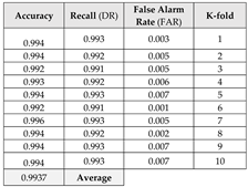 |
Table 17.
Evaluation of the performance of the combined method with the Nearest Neighbor method, Support Vector Machine, and improved Random Neural Network on DS2OS dataset.
Table 17.
Evaluation of the performance of the combined method with the Nearest Neighbor method, Support Vector Machine, and improved Random Neural Network on DS2OS dataset.
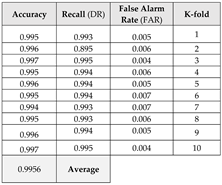 |
Table 18.
Comparing tested methods and proposed model using DS2OS dataset.
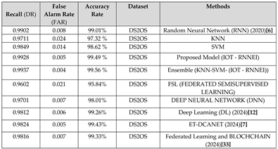 |
Table 19.
Comparison of the tested methods and the proposed model on CIC-IDS2018 dataset.
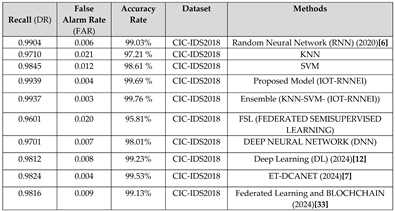 |
Table 20.
Comparison of the tested methods and the proposed model on CIC-IOT2023 dataset.
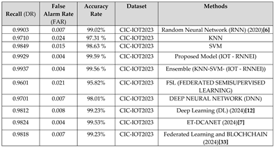 |
Table 21.
Comparison of training time and classification accuracy in the random neural network (RNN) and proposed model (IOT - RNNEI) on DS2OS dataset.
Table 21.
Comparison of training time and classification accuracy in the random neural network (RNN) and proposed model (IOT - RNNEI) on DS2OS dataset.
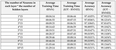 |
Disclaimer/Publisher’s Note: The statements, opinions and data contained in all publications are solely those of the individual author(s) and contributor(s) and not of MDPI and/or the editor(s). MDPI and/or the editor(s) disclaim responsibility for any injury to people or property resulting from any ideas, methods, instructions or products referred to in the content. |
© 2024 by the authors. Licensee MDPI, Basel, Switzerland. This article is an open access article distributed under the terms and conditions of the Creative Commons Attribution (CC BY) license (http://creativecommons.org/licenses/by/4.0/).
Copyright: This open access article is published under a Creative Commons CC BY 4.0 license, which permit the free download, distribution, and reuse, provided that the author and preprint are cited in any reuse.


