
Submitted:
08 November 2024
Posted:
12 November 2024
You are already at the latest version
Abstract
In this paper, we propose the Fuzzy formulation of the classic Frankot-Chellappa method by which surfaces can be reconstructed using normal vectors. In the Fuzzy formulation, the surface normal vectors may be uncertain or ambiguous. The underlying model yields a Fuzzy Poisson partial differential equation, where it is imperative to give meaningful representations of Fuzzy derivatives. The solution of the resulting Fuzzy model is approached numerically. To this end, a fuzzy formulation for the discrete sine transform method is explored, which results in a fast, accurate and robust method for surface reconstruction. In experiments we consider specifically the robustness with respect to noisy surface normal vectors.
Keywords:
Surface normal integration
; Frankot-Chellappa method
; Fuzzy derivatives
; Fuzzy partition
; Fuzzy Poisson equation
1. Introduction
The integration of surface normals for the purpose of computing the shape of the corresponding surface in 3D space is a classic problem in computer vision [10]. Many methods have been proposed with the aim to devise an approach that combines accuracy, robustness with respect to noise in the data and computational efficiency, see e.g. [3,4,6,7,9,14] as well as the survey paper [11]. It appears evident that even nowadays it is still a challenging task to devise a method that is highly accurate and offers at the same time robustness and computational efficiency.
When it comes to computational efficiency, the classic method of Frankot and Chellappa [7] is still among the most powerful methods. It relies on a finite difference approximation of a Poisson equation which naturally arises in the problem formulation of surface normal integration. The crucial part of the Frankot-Chellappa algorithm is the use of a discrete sine transform for dealing with the surface normal data in the Poisson model. However, it is well-known that the classic Frankot-Chellappa method does not incorporate a mechanism that deals with noisy data, and also accuracy issues may arise in the vicinity of steep surface gradients.
Fuzzy concepts apply human reasoning ability to knowledge-based systems. When the assumptions of the problem have uncertainty, one consider a fuzzy interpretation of parameters or data. Due to uncertainty e.g. due to noise in image acquisition systems, in many aspects of image processing fuzzy processing may be desirable.
As indicated, the underlying problem formulation in the classic method from Frankot and Chellappa a Poisson equation needs to be solved, for which the discrete sine transform can be explored.
In this research, a fuzzy formulation of the classic Frankot-Chellappa model and algorithm for surface normal reconstruction is presented. It turns out that the main methodology from the classic scheme, namely exploring the discrete sine transform, can be transferred to the fuzzy formulation in terms of the fuzzy sine transform. Our fuzzy extension appears to be fast, accurate, and nearly robust to noisy data. The technique of fuzzy transform (F-transform for short) has been introduced by I. Perfilieva et al in [12,13]. Similarly to the classic sine transform it can be cast in two ways, as a direct or an inverse transform. The authors of that work have proved that the inverse F-transform has good approximation properties and is relatively easy to use. As for the fuzzy formulation of the Poisson equation, fuzzy partial differential equations (PDEs) have been introduced in the past. In 2018, the fuzzy Poisson equation with Dirichlet boundary conditions has been discussed, proving uniqueness and stability of a solution in [8]. We explore the use of this recent concept in the current paper. As for a potential benefit of our developments, we study the possible enhanced robustness of the fuzzy formulation to noise. This may be considered to be sometimes a more delicate issue with the classic method that does not assume uncertain data.
2. Fuzzy Concepts
The purpose of this section is to present the necessary fuzzy notions and concepts for use with this paper.
2.1. Fuzzy Numbers and Fuzzy Partition
We write , a number in , for the fuzzy membership function evaluated at x. An -cut of , written , is defined as , for . The Triangular Fuzzy Number (TFN) is defined by three numbers , where the graph of , the membership function of the fuzzy number , is a triangle with the base on the interval and vertex at . We specify as .
By cosidering the membership function of is defined as:
Given two TFNs and , their arithmetic addition is a TFN:
Also the -difference , is a TFN.
Let us consider the fuzzy partition [12]: choose an interval as a universe, and assume that a function f is given at points
Below, we recall the definition of a fuzzy partition. Let be fixed nodes within . Fuzzy sets identified with their membership functions , defined on , establish a fuzzy partition of if they fulfill the following conditions for :
The membership functions are called basic functions.
We say that the fuzzy partition given by , is an h-uniform fuzzy partition if the nodes are equidistant, and two additional properties are met:
2.2. The F-Transform
Consider the discrete F-transform [12]: the fuzzy sets establish a fuzzy partition of and is a discrete real valued function defined on the set where .
The following vector of real numbers is the (direct) discrete F-transform of f w.r.t. where the k-th component is defined by
The inverse discrete F-transform reads as:
For h-uniform fuzzy partition of , there exists an even function :
The points are equidistant in the interval and moreover , where m and l are connected by the following equality: . Thus chosing points it is assured that the nodes are among them, i.e. for each there exists j such that .
Similarity to the case of a function of one variable we can have F-Transform in 3D. Let a function f be given at nodes , and , where , , be basic functions which form fuzzy partitions of and , respectively. Suppose that sets P and Q of these nodes are sufficiently dense with respect to the chosen partitions.
We say that the -matrix of real numbers is the discrete F-transform of f with respect to and if
holds for all
The elements , , are called components of the F-transform.
Let and be basic functions which form fuzzy partitions of and respectively. Let f be a function from and be the F-transform of f with respect to and . Then the function
holds for all .
2.3. Fuzzy Partial Derivatives
A fuzzy-valued function f of two variables is a rule that assigns to each ordered pair of real numbers, , in a set D a unique fuzzy number denoted by . The set D is the domain of f and its range is the set of values that f takes on, that is, .
We show the parametric representation of the fuzzy-valued function by , for all and .
Let . Then the first generalized Hukuhara partial derivatives (-derivatives for short) of a fuzzy-valued function at with respect to variables x, y are the functions and given by
provided that and in F where is the gH-difference.
3. Classic Frankot-Chellappa Surface Normal Integration
Let us briefly recall the classic Frankot-Chellappa method. For a given normal field with and the surface is sought, such that the vector is orthogonal to the surface at the point . Therefore
Now, in order to numerically approximate a solution of this equation, one may try to find a function z such that the distance between and g in the display space of the surface is small. The necessary condition for z being a minimizer of the distance over all can be written as that is a Poisson PDE. For approximation of partial derivatives, one may consider
Now by using the inverse discrete sine transformation one may obtain
Where and are the discrete sine transform of f and z and
4. Fuzzy Poisson Equation
Numerous problems in industry lead to an equation with fuzzy partial differential equation in the following form:
in which is a regular area, and is a fuzzy known function. Since is a fuzzy function and coefficients in are fuzzy, then according to the extension principle is a fuzzy function too.
For the first-order derivatives based on we have:
Here we assume the is a symmetric triangular fuzzy number, and we write , when .
Now for a normal field with , we assume as a symmetric triangular fuzzy number with vertex , also for with vertex , and with vertex . (we can suppose the fuzziness between 0 and 1 here is supposed )
We now consider the underlying PDE as a fuzzy partial differential equation:
By replacing fuzzy second-order derivative in definitions in previous sections and fuzzy Poisson equation , in a similar way as M. Abdi et al. in [1] has obtained by discrete partial difference expressions, we will have:
By entering the derivatives in the Poisson equation, we reach its discrete formula:
Then
5. Summary of Fuzzy Frankot-Chellappa Method
In the following we only consider problems with Dirichlet boundary conditions and write the right-hand side more generally as a function , so that we are looking for a solution of . For this we use the inverse discrete sine transformation and :
First we solve it only with a homogeneous Dirichlet condition for , where , in order to later determine the solution for problems with an inheterogeneous Dirichlet situation using the knowledge gained.
We again insert the inverse transform from (8) into the discrete formula (7), leaving h undetermined:
Then, we have
If u and k are not in and v and l are not elements of , we have
Where and are the discrete fuzzy sine transform of and and
.
6. Experimental Results
In this section, we investigate our method with using fuzzy concepts. We consider experiments for surface reconstruction using normal vectors, some of which are uncertain normal vectors or ambiguous, and observe if this leads to better results in terms of accuracy or noise suppression due to noisy data.
6.1. Comparison in Terms of Accuracy
Now, to compare the responses obtained from the classical and fuzzy methods, we first use de-fuzzification, then we calculate the difference of all points in the classical solution and compare the de-fuzzified solution with the exact solution.
For every , where we use for that is obtained by sine discrete transform and , the de-fuzzified solution from , is obtained by fuzzy sine discrete transform. The de-fuzzification method that is used here is .
In Table 1 we compare exact function, discrete sine transformation approximation and the obtained result from de-fuzzification of fuzzy sine discrete transformation approximation (with ) for four cases. In Figure 1 we compare exact function, discrete sine transformation approximation and -cut of fuzzy discrete sine transformation approximation () for three cases of the above examples that is done on the rectangle :
6.2. Comparison with Respect to Noise Suppression
Since the operation on the function is linear, it makes sense to consider to fuzzify the elements of normal vectors at the beginning of the operation, and then de-fuzzify at the end, so the calculation error is almost the same in the two approximations.
A possible advantage by fuzzy construction of our method is in its application at specific points without given data (i.e. holes in domain where data is given). Also integration with fuzzy components may potentially remove noise better than classic method. Which we confirm in Figure 2 where we have solutions with noise for cases in Figure 1.
To be more precise, it has been proved in [13] that the inverse F-transform of a noisy function is almost equal to the inverse F-transform of the original function. Which makes us conjecture that our method has good denoising capabilities.
We consider a noise, represented by a function and is the representation of the noised function z. On the basis of linearity of the direct F-transform, this noise can be removed if its regular components of the direct F-transform are equal to zero. Here we consider to apply both F-transform (direct and inverse) to a function to remove a certain noise. Indeed, the inverse F-transform can be considered as a special fuzzy identity filter which can be utilized.
Let a discretization for the surface with size be represented a function of two variables defined at nodes . The F-transform (2.3) for is as follows:
Where , , , , are basic functions which form fuzzy partitions of and , respectively. A reconstruction of the image z, being described by with respect to and , can then be computed by the inverse F-transform (2.4) adapted to the domain :
which holds for all . Also, we know that has improved in [13], where the noise be continuous functions on . We can see in Figure 3 that F-transform performs as an effective filter.
We also have constructive suggestions for specific situations that occur in reality, for example, a part of the procedure cannot be reconstructed due to insufficient information. In this way, to make the components of the normal vector of points with unknown normal, the corresponding directions are used , and . In fact, in every point in area with uncertain normal vector for the of the unknown point, we use the information of the closest point in the x-direction, and for the , we use the information of the closest point in the y-direction.
Then get changed as follow:
7. Conclusion
In this paper, the Fuzzy Poisson equation with Dirichlet boundary conditions was investigated as part of a fuzzy Frankot-Chellappa method. We show experimentally, backed up by some theoretical considerations, that our fuzzy Frankot-Chellappa method reconstructs surfaces, using normal vectors of which some may be considered uncertain or ambiguous, with reasonable results. In terms of accuracy, for smooth surfaces our fuzzy method gives equivalent results than the classic method, while in terms of noise suppression the use of fuzzy concepts appears to be beneficial.
To achieve these results, some concepts such as a fuzzy-valued vector function, fuzzy operators, and a fuzzy sine discrete transform were studied. Consequently, the fuzzy solution of the fuzzy Poisson equation was obtained by our applying an fuzzy extension of .
For future research, other types of fuzzy numbers may be used. We may consider also using fuzzy distance between fuzzy normal vectors to can obtain missed normal vectors for approximating related surface with missing data.
References
- M. Abdi, T. Allahviranloo, Fuzzy finite difference method for solving fuzzy Poisson equation. Journal of Intelligent and Fuzzy Systems 2019, 37, 5281–5296. [CrossRef]
- T. Allahviranloo, Difference methods for fuzzy partial differential equations. Comput. Methods Appl. Math. 2006, 2, 233–242.
- M. Bähr, M. Breuß, An Improved Eikonal Method for Surface Normal Integration, Proceeding of the 37th German Conference on Pattern Recognition. Aachen, Germany (2015).
- M. Bähr, M. Breuß, Y. Queau, A.S. Boroujerdi J.D. Durou, LU-Fast and accurate surface normal integration on non-rectangular domains. Comput. Vis. Media. 2017, 3, 107–129. [CrossRef]
- J.D. Durou, J.F. Aujol, F. Courteille, Integrating the normal field of a surface in the presence of discontinuities. Energy Minimization Methods Comput. Vis. Pattern Recogn. 2009, 5681, 261–273.
- D. Dubois, H. Prade, Operations on fuzzy numbers. International Journal of Systems Science 1978, 9, 613–626. [CrossRef]
- R.T. Frankot, R. Chellappa, A method for enforcing integrability in shape from shading algorithms. IEEE Trans. Pattern Anal. Mach. Intell. 1988, 10, 576–593.
- R. Ghasemi Moghaddam, T. Allahviranloo, On the fuzzy Poisson equation. Fuzzy Sets Syst. 2018, 347, 105–128. [CrossRef]
- M. Harker, P. O’ Leary, Least squares surface reconstruction from measured gradient fields, In: Proceedings of the IEEE Conference on Computer Vision and Pattern Recognition., (2008).
- B.K.P. Horn, Robot Vision, McGraw-Hill Book, (1986).
- Y. Queau, J-D. Durou, J-F. Aujol, Normal Integration: A survey. J Math Imaging Vis. 2018, 60, 576–593. [CrossRef]
- I. Perfilieva, Fuzzy transforms: Theory and applications. Fuzzy Sets Syst. 2006, 157, 993–1023. [CrossRef]
- I. Perfilieva, P. Valášek, Fuzzy Transforms in Removing Noise, in Computational Intelligence, Theory and Applications, International Conference 8th Fuzzy Days, Dortmund, Germany, (2004).
- T. Simchony, R.T. Frankot, Direct analytical methods for solving poisson equations in computer vision problems. IEEE Trans. Pattern Anal. Mach. Intell. 1990, 12, 435–446. [CrossRef]
Figure 1.
Comparison of exact function, discrete sine transformation approximation (sT) and -cut components of the fuzzy sine discrete transformation approximation (FsT), with for : . We confirm here that the accuracy of the fuzzy approximation is equivalent to the classical approximation .
Figure 1.
Comparison of exact function, discrete sine transformation approximation (sT) and -cut components of the fuzzy sine discrete transformation approximation (FsT), with for : . We confirm here that the accuracy of the fuzzy approximation is equivalent to the classical approximation .
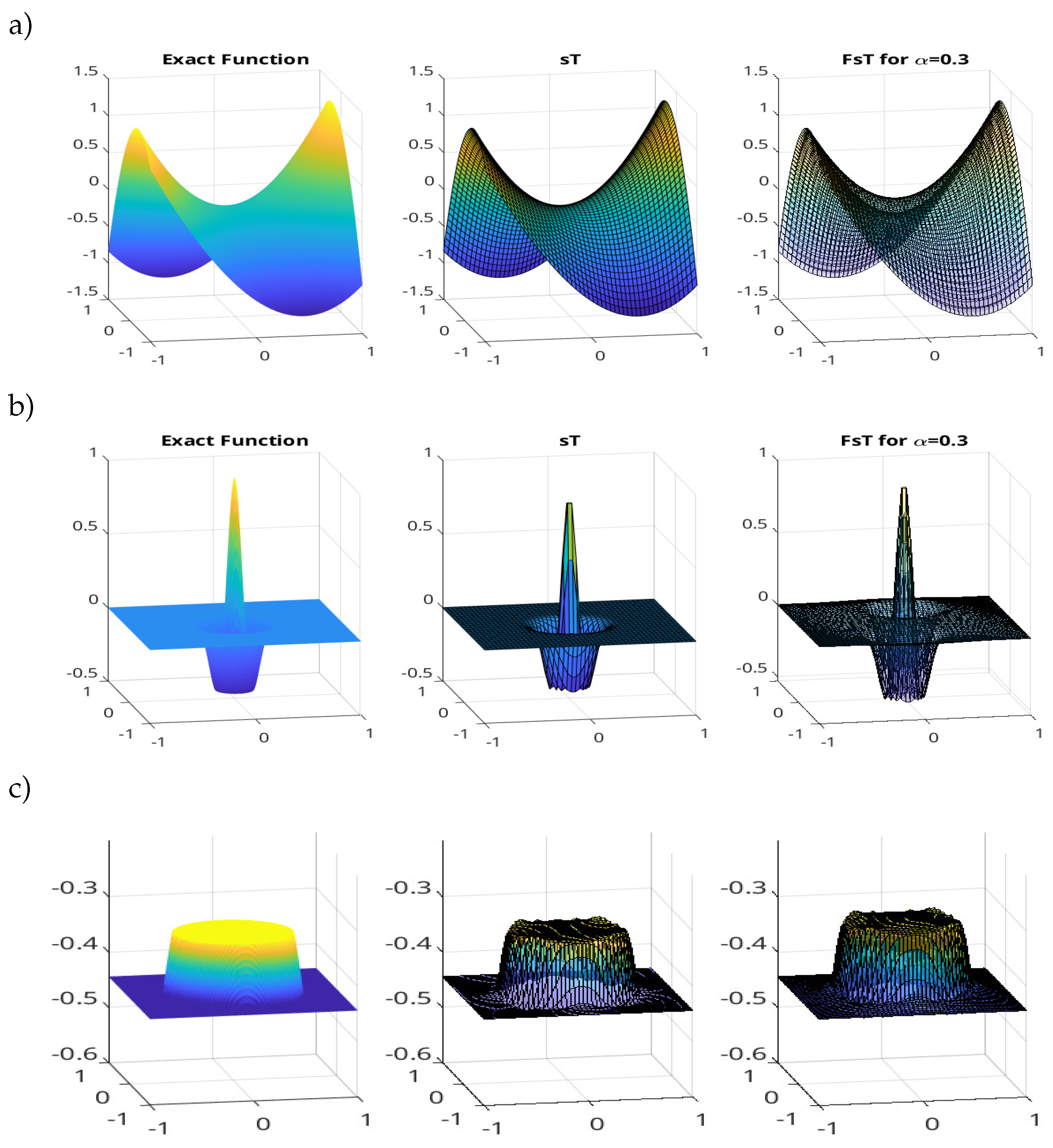
Figure 2.
The solution with noise for three cases in Figure 1. As it shows, fuzzy approximation is better to suppress noise than classic approximation since .
Figure 2.
The solution with noise for three cases in Figure 1. As it shows, fuzzy approximation is better to suppress noise than classic approximation since .
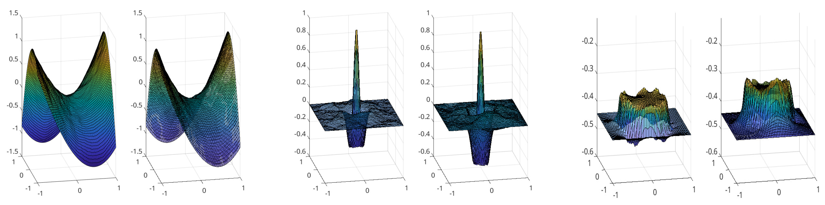
Figure 3.
Removing noise with "F-transform" in order to obtain . As it shows, fuzzy approximation is better to suppress noise than classic approximation since .
Figure 3.
Removing noise with "F-transform" in order to obtain . As it shows, fuzzy approximation is better to suppress noise than classic approximation since .
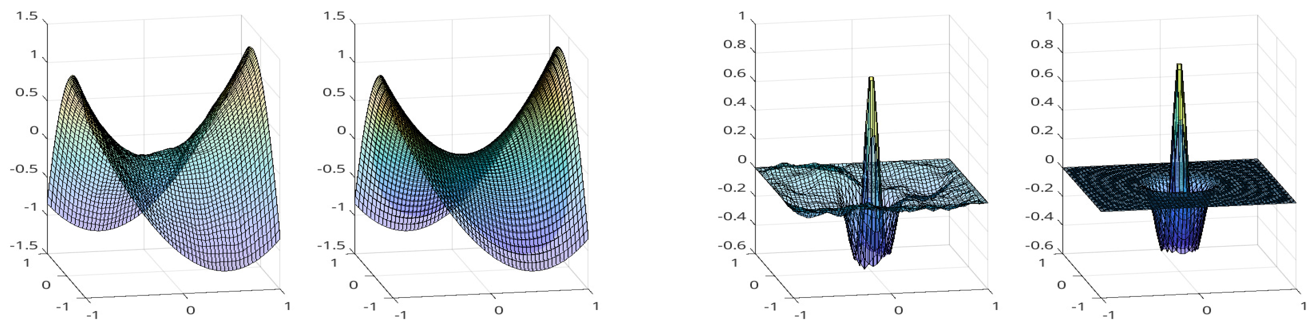

Table 1.
Compare the classical and fuzzy methods with and .
| Exact function z | d | D | d(noise ) | D(noise ) |
|---|---|---|---|---|
| 0.5704e-06 | 0.5704e-06 | 1.9234e-02 | 4.4535e-03 | |
| 1.1119e-06 | 1.1119e-06 | 2.6299e-03 | 1.6738e-03 | |
| 4.0103e-06 | 4.0103e-06 | 3.1116e-03 | 4.4851e-04 | |
| 8.3435e-05 | 8.3435e-05 | 4.4281e-04 | 7.3650e-05 |
Disclaimer/Publisher’s Note: The statements, opinions and data contained in all publications are solely those of the individual author(s) and contributor(s) and not of MDPI and/or the editor(s). MDPI and/or the editor(s) disclaim responsibility for any injury to people or property resulting from any ideas, methods, instructions or products referred to in the content. |
© 2024 by the authors. Licensee MDPI, Basel, Switzerland. This article is an open access article distributed under the terms and conditions of the Creative Commons Attribution (CC BY) license (http://creativecommons.org/licenses/by/4.0/).
Copyright: This open access article is published under a Creative Commons CC BY 4.0 license, which permit the free download, distribution, and reuse, provided that the author and preprint are cited in any reuse.