PreKiCan: A PARAM Utkarsh-Powered Model for Early Kidney Cancer Identification

Shubham Ranswal

doi:10.20944/preprints202411.0694.v1

Submitted:

10 November 2024

Posted:

11 November 2024

You are already at the latest version

Abstract

The early detection of kidney cancer significantly increases the chances of better and successful treatment and obviously impacts patient’s survival. We conducted research that leverages the cutting-edge capabilities of the PARAM Utkarsh supercomputer, maintained by C-DAC Bangalore, to enhance the accuracy and speed of kidney cancer detection from x-ray images. We developed a deep learning binary classification model, that demonstrates a remarkable peak prediction accuracy of 99.8%, achieved through training with 250 epochs in high performance computing environment. The model incorporates the ultimate processing power of supercomputing to efficiently manage large datasets and perform complex computations, providing a remarkable improvement over traditional diagnostic method. This paper demonstrates the model development process within the high-performance computing environment and highlights the potential impact for the same in medical field, focusing the power of supercomputing technology in improving medical diagnostic processes and their outcomes in healthcare, to be more accurate.

Keywords:

Kidney Cancer Detection

;

Deep Learning

;

Supercomputing

;

PARAM Utkarsh Supercomputer

;

Image Classification

;

Artificial Intelligence in Healthcare

;

High Performance Computing

Subject:

Computer Science and Mathematics - Artificial Intelligence and Machine Learning

Introduction

The integration of supercomputing technology in healthcare represents a huge shift towards more accurate as well as fast diagnostic capabilities. Supercomputers, with their ultimate processing power and capabilities, offer the potential to handle huge datasets and perform complex computations that are beyond the scope of our conventional computing systems. This capability is significantly important in the field of medical sciences, where time-sensitive and data-intensive tasks, such as medical imaging and genetic sequencing, require both precision as well as efficiency.

The ability of machine learning and artificial intelligence has further impacted the utility of supercomputers in medical diagnostics. These technologies allow the development of computational models that can be learned by themselves, be it images, text or anything else, that improves accuracy, precision, and the adaptability of the model, over time. By incorporating such advancements, healthcare professionals can achieve earlier and more accurate disease detection, improving patient’s conditions and decreasing the overall mortality rate.

This research employs the PARAM Utkarsh Supercomputer, a state-of-the-art high performance computing system at C-DAC, Bangalore. Established as part of the Government of India’s National Supercomputing Mission, the state-of-the-art facility aims to enable researchers, scientists and engineers to provide state-of-the-art computing capabilities for a wide range of applications.

Table 1. PARAM Utkarsh System Configurations.

Component	Value
Theoretical Peak Floating-point Performance Total	838 TFLOPS ((peak)
Base Specifications (Compute Nodes)	2 X Intel Xeon Cascadelake 8268, 24 Cores, 2.9 GHz, Processors per node, 192 GB Memory, 480 GB SSD
Master/Service/Login Nodes	10 nos
CPU only Compute Nodes (Memory)	107 nos. (1928)
GPU Compute Nodes (Memory)	10 (192 GB)
High Memory Compute Nodes	39 nos. (768GB)
Total Memory	52.416 TB
Interconnect	Primary: 100Gbps Mellanox InfiniBand Interconnect network 100% non-blocking, fat tree topologySecondary: 106/16 Ethernet NetworkManagement network: 16 Ethernet
Storage	1PB PFS based storage

This high-performance system is equipped with the latest technology that gives it an exceptional lead in overall performance. It is based on an Intel Cascade Lake processor and an NVIDIA Tesla V100 GPU. It has more than 50,000 computer cores and a liquid cooling system for efficient PUE. It supports high-speed, non-blocking InfiniBand connections of approximately 100 Gbps for smooth and easy data transfer. It has a maximum computing capacity of 838 teraflops.

The range of services PARAM Utkarsh is equipped with is designed to meet various user needs including services like HPC and Storage Services, Big Data Cluster Service, Cloud Services, AI capability through ML/DL framework, secure infrastructure, high availability and stability and reliability, application activation and user support and training. By harnessing the power of PARAM Utkarsh, MSMEs and startups in India can significantly reduce their time to market for new products and services and increase their innovation potential through better simulations and data analytics.

PARAM Utkarsh acts as a catalyst for innovation and research in a variety of sectors in India. It supports academia through cutting-edge research in science, engineering and medicine; Industry by overcoming barriers to innovative modern technology, optimizing processes and increasing competitiveness; Government by supporting policymaking, decision-making and solving complex societal challenges; MSMEs and start-ups get access to world-class computing resources that many may not be able to afford without.

This is one of the key factors in India’s transformation into a digital economy in its quest to innovate the world’s technology. That is why PARAM Utkarsh comes in handy for many and is in demand. It offers great features and state-of-the-art infrastructure to accelerate the process of innovation, scientific research and technological improvement in India, making it even more internationally competitive.

In this study, we focus on applying deep learning algorithm to predict kidney cancer from x-ray images. The choice of using the PARAM Utkarsh Supercomputer is strategic, leveraging its computational resources to process huge volumes of image data, enabling the training of a highly accurate binary classification model. The aim of this study is to demonstrate how supercomputing can significantly enhance the capabilities of predictive models in medical diagnostics, offering valuable insights that are not only rapid but also reliable. In the next sections, we have covered a review of already published works in this sector, the detailed methodology followed by this work, results, discussions and conclusions.

Literature Review

Nicholas J Vogelzang [1], in one of his studies, highlighted that Early-stage kidney cancer is treated with radical nephrectomy, but in certain circumstances a partial nephrectomy may be performed. In some other published work, Wong-Ho Chow [2] mentioned that Kidney cancer in adults originates from the renal parenchyma (adenocarcinoma cell type [RCC]) or renal pelvis (transitional cell type [rTCC]); RCC is the main type of kidney cancer. We already know that kidney cancer is one of the most dangerous and common cancers across the world. In the previously presented studies [3–7], authors made the use of metabolomic techniques to identify metabolites from the urine sample of kidney cancer patients.

A study authored by Seda Arslan Tuncer [8] proposed a decision support system that detected renal cell cancer taking spinal cord as the point of reference in image segmentation, based on Support Vector Machine (SVM) and K-Means. Hadjiyski [9] proposed a Deep Learning Neural Network model that distinguished kidney cancer stages from stage 1 to stage 2, 3 and 4. It supported early detection of kidney cancer as it significantly supported detection of disease and prevention of organs. Also, distinguishing stages supported in better diagnosis as it provided a breakthrough, now it was clear as the medical staff should proceed with chemotherapy or there is scope for organ preservation. They considered Computer Tomography (CT) scans of 227 real patients from the Cancer Imaging Archive TCIA database and obtained area under the ROC curve (AUC) of 0.97 for training sets, 0.91 for validation sets and 0.90 for the test sets.

A study published in the journal named Computers in Biology and Medicine used KiTS19 dataset of 300 CT scans, and managed to obtain the sensitivity of 97.42%, specificity of 99.94% and the peak accuracy of 99.92%. In another study published by Acta Radiologica proposed a model for kidney segmentation and kidney tumor detection on abdominal computed tomography (CT) scans. They considered 12 cases of kidney tumors, spanning 156 transverse images and attained a sensitivity of 85% with 0% false positive results [11]. Along with all these, a published work by Zhang et al, [12] says that MR imaging and ultrasound function as valuable problem-solving tools for medical imaging of cancer patients.

Asha, V., et al, in their published work at IITCEE 2024 [13], proposed an enhanced hybrid deep learning model for kidney cancer image categorization. They combined IAO and ResNet101 to support the peak precision of 98.90% overall. A group of researchers Uhm, KH., Jung, SW., Choi, M.H. et al. [14], the authors proposed a unified framework to identify and classify the subtypes for diagnosis without human involvement. They trained the model using 308 patients CT data, collected from St. Mary Hospital, who underwent nephrectomy for renal tumors. Finally, they achieved AUC of 0.889, and outperformed radiologists for several subtypes.

A study published in the International Journal of Engineering Research and Development [15] provided information about several sources and causes to help the patients who are dealing with the diagnostic challenges of Kidney Cancer, that is serving as the guide of principles of kidney cancer.

Methodology

This section presents the comprehensive methodology we followed to develop and validate our deep learning model for the prediction of kidney cancer (or we can say kidney tumor), from the x-ray images, utilizing the super computational capabilities of PARAM Utkarsh Supercomputer.

Data Collection and Preparation

The initial phase involved collecting a large dataset of x-ray images from various publicly available medical imaging databases. Kaggle is an online platform that organizes several online competitions in the field of data science, artificial intelligence and machine learning for people throughout the globe. Medical Scan Classification Dataset [16], last updated in December 2023, is a publicly available dataset on Kaggle, that was used for model development. This dataset comprises of a huge number of X-Ray Images that can be used to classify Kidney Cancer, Cervical Cancer, Alzheimer’s, Covid 19, Pneumonia, Tuberculosis, Monkeypox, Malaria and for preprocessing Chest X-Ray it has Bone Shadow Suppression Dataset, with a total of 137,000 image files collectively. Out of which, specifically, 10,000 images were taken into consideration for this study to predict Kidney Cancer optimally.

The dataset was equally balanced between cancerous and non-cancerous cases to mitigate model bias as 5000 cancerous and 5000 non-cancerous images were taken into consideration. A sample cancerous (Figure 1) and non-cancerous (Figure 2) images are as follows. The directory named validation and train are provided during model initialization step. Data preprocessing was performed by resizing images to a uniform size of 150x150 pixels, normalizing pixel values, and augmenting the dataset through various techniques such as rotation, zoom, and horizontal flipping to increase the robustness of the model against different orientations and sizes of tumors.

Model Architecture

The architecture of the deep learning model is crucial for its ability to accurately classify x-ray images into cancerous and non-cancerous categories. For this project, we designed a convolutional neural network (CNN) tailored to the specific requirements of medical image analysis, particularly for kidney cancer detection. The model flow for “PreKiCan,” a convolutional neural network (CNN) designed for the early detection of kidney cancer from x-ray images, is systematically outlined in a comprehensive flowchart, given in Figure 3.

This flowchart delineates the entire process from data input through model training to making predictions. This model flow is integral to understanding how the convolutional neural network processes and analyzes x-ray images to deliver predictions. The efficiency and accuracy of “PreKiCan” in detecting early signs of kidney cancer underscore the potential of deep learning in medical diagnostics, leveraging the computational power of high-performance computing systems like the PARAM Utkarsh Supercomputer.

This CNN architecture is compiled with the Adam optimizer, a popular choice for deep learning applications due to its efficient computation of large datasets and adaptive learning rate capabilities. The loss function used is binary crossentropy, which is appropriate for binary classification tasks like this one. The proposed algorithm outlines a comprehensive process for detecting kidney cancer using a deep learning convolutional neural network (CNN), designed to analyze x-ray images. The algorithm is structured into five main steps, encompassing data preparation, model architecture, compilation, training, and evaluation/prediction phases. Each step is crucial in building a robust model that leverages deep learning techniques for medical imaging analysis, aiming to classify images into binary categories: cancerous or non-cancerous.

Table 3. PreKiCan Algorithmic Structure.

Input: Set of x-ray images.
Output: Prediction whether the x-ray image indicates presence of kidney cancer (binary output: cancerous or non-cancerous).

Step 1: Data Preparation

I)

Load Dataset: Import x-ray image dataset.

II)

Preprocessing:

i.: Normalize the pixel values (scale between 0 and 1).
ii.: Augment the data to increase dataset size and variability using techniques such as rotation, width shift, height shift, and horizontal flipping.

Step 2: Model Architecture: Layer Setup

I): Conv2D Layer 1: Apply 32 filters with a 3x3 kernel size, using ReLU activation.
II): MaxPooling2D Layer 1: Apply pooling operation with a 2x2 pool size to reduce dimensionality.
III): Conv2D Layer 2: Increase to 64 filters, 3x3 kernel size, ReLU activation.
IV): MaxPooling2D Layer 2: Apply pooling operation with a 2x2 pool size.
V): Conv2D Layer 3: Increase to 128 filters, 3x3 kernel size, ReLU activation.
VI): MaxPooling2D Layer 3: Apply pooling operation with a 2x2 pool size.
VII): Conv2D Layer 4: Increase to 128 filters, 3x3 kernel size, ReLU activation.
VIII): MaxPooling2D Layer 4: Apply pooling operation with a 2x2 pool size.
IX): Flatten Layer: Flatten the output of the last pooling layer to form a 1D vector.
X): Dense Layer 1: Apply a dense layer with 512 neurons, ReLU activation.
XI): Dense Layer 2 (Output Layer): Apply a dense layer with 1 neuron, sigmoid activation function for binary classification.

Step 3: Compilation

I): Optimizer: Use Adam optimizer for efficient gradient descent.
II): Loss Function: Use binary crossentropy as it is suitable for binary classification problems.
III): Metrics: Track accuracy of the model during training and validation.

Step 4: Training

I): Feed the training data into the model.
II): Set the number of epochs (e.g., 250 as per your setup).
III): Define the batch size (e.g., 32).
IV): Use validation data to tune hyperparameters and prevent overfitting.

Step 5: Model Evaluation and Prediction

I)

Save Trained Model: Save the model weights and architecture in ‘model.h5’.

II)

Load Model for Prediction: Use ‘predict.py’ to load ‘model.h5’ and make predictions.

III)

Make Predictions:

Input new x-ray images.
Preprocess them as done in training.
Model predicts ‘cancerous’ or ‘non-cancerous’ based on learned features.

This algorithm represents a sophisticated approach to medical diagnostics, leveraging the power of deep learning to enhance accuracy and efficiency in cancer detection. It reflects a significant application of AI technology in healthcare, aiming to provide faster, non-invasive diagnostics that can potentially save lives by enabling early detection and treatment of kidney cancer.

Model Training

Training the deep learning model effectively is crucial for achieving high accuracy and reliability in medical diagnosis. This section details the setup and execution of the training phase for the convolutional neural network designed to detect kidney cancer from x-ray images. The binary classification model, based on Convolutional Neural Network (CNN), is primarily designed to recognize patterns and features in images. The architecture consists of multiple convolutional layers followed by pooling layers, dropout layers to prevent overfitting, and fully connected layers for binary classification. The model was implemented using TensorFlow and Keras libraries. Along with these, Pillow is another python library that was used to train the model that enables image manipulation with python. A detailed breakdown of these layers is as follows:

I).: Conv2D: The first Conv2D layer has 32 filters of size 3x3 and uses ReLU (rectified linear unit) activation. It also specifies the input shape of the image. Subsequent Conv2D layers have 64 and 128 filters respectively, also using 3x3 filters and ReLU activation. These layers increase the depth of the feature maps as we progress deeper into the network.
II).: MaxPooling2D Layers: These layers reduce the spatial dimensions (width and height) of the input volume for the next convolution layer. They perform down-sampling by dividing the input into rectangular pooling regions and outputting the maximum of each region. We used a pool size of 2x2. This helps reduce computation, as well as helps make feature detectors more invariant to small changes in position.
III).: Flatten Layer: After the last MaxPooling layer, a Flatten layer is used to convert the 3D feature maps into 1D feature vectors. This layer prepares the spatially arranged data into a form suitable for classification.
IV).: Dense Layers: These are fully connected layers that follow the Flatten layer. They perform classification based on the features extracted and down sampling. A Dense layer with 512 units and ReLU activation is serving as a fully connected layer that can learn non-linear combinations of the high-level features as represented by the flattened vector from the previous layer. The final Dense layer with 1 unit and a sigmoid activation function, which is typical for binary classification tasks. This layer outputs a probability indicating the presence or absence of kidney cancer.

These layers are stacked sequentially to form a model that can effectively learn from image data to perform binary classification tasks, such as your application in predicting kidney cancer. PreKiCan was trained on the PARAM Utkarsh Supercomputer [17], Utilizing its advanced computational capabilities to manage the intensive demands of deep learning. The training configuration was as follows:

Epochs: The PreKiCan was trained for 250 epochs, allowing sufficient time to learn from the data thoroughly. An epoch represents one complete pass of the training dataset through the algorithm.
Batch Size: A batch size of 32 was chosen. This size is a balance between training speed and model performance, providing a stable gradient update during training.
Optimizer: The Adam optimizer was employed for its efficiency in handling sparse gradients and adaptive learning rate capabilities, which are beneficial for converging faster to the optimal weights.
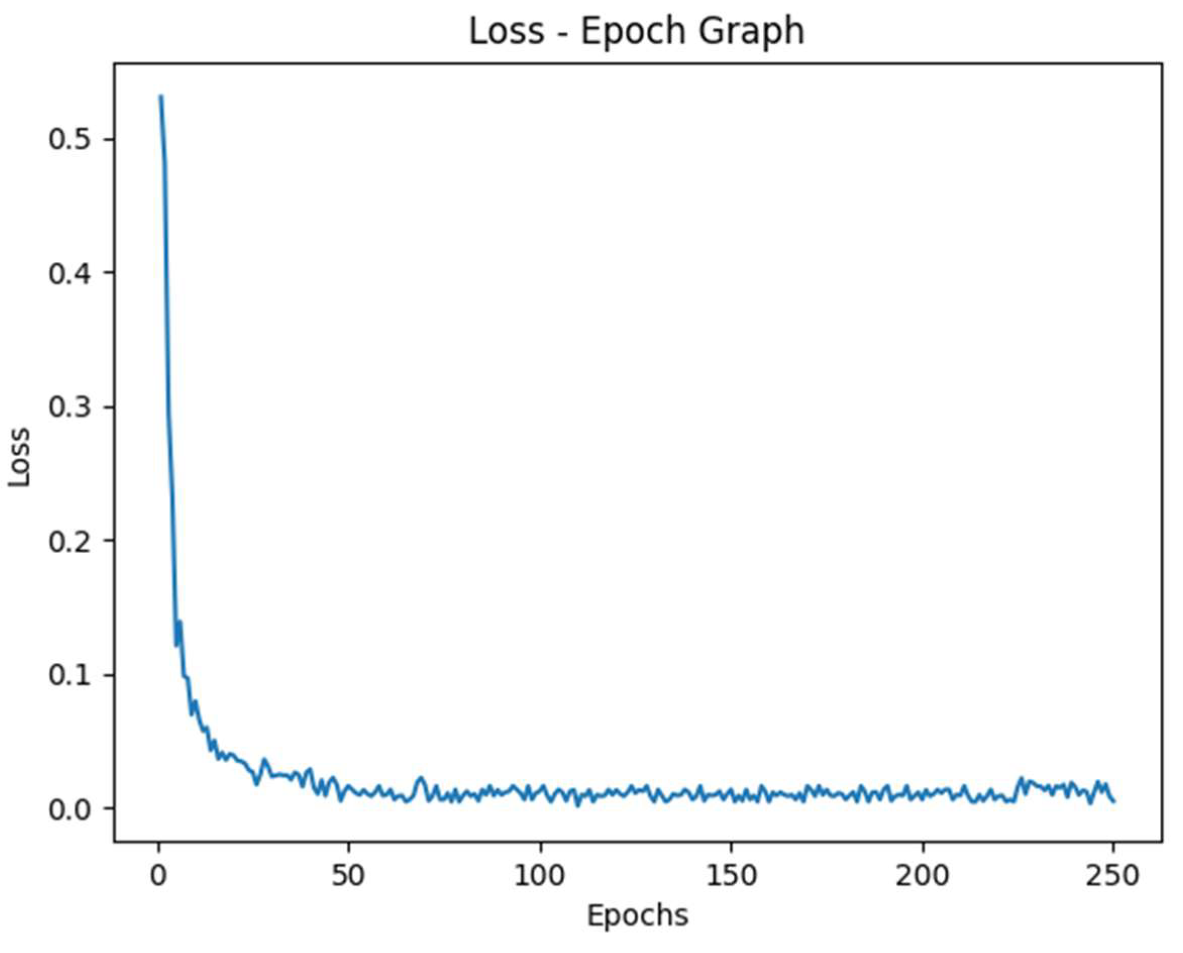
Loss Function: Binary crossentropy was used as the loss function, which is standard for binary classification tasks. It measures the performance of the model whose output is a probability value between 0 and 1.

After each epoch, the model’s performance was evaluated using a portion of the dataset reserved for validation.

Validation and Testing

After the model training was complete, the final step was to test the model using a separate testing set, which was also withheld from the training dataset to ensure the integrity of the tests. Model validation was performed using a separate set of images, constituting 20% of the total dataset, which was not exposed to the model during the entire training phase. This approach ensured that the evaluation metrics, primarily accuracy. Out of total 10,000 images, we had 5000 cancerous and 5000 non-cancerous images, that were randomly distributed into an 80:20 to train and validation phases. On analyzing the different records obtained, the following confusion matrix (Figure 4) and classification report (Table 4) was obtained.

Computational Environment

The computational power of the PARAM Utkarsh Supercomputer was used to manage the high computational demands of model training and testing. The supercomputer’s specifications, which include high memory and multi-GPU configurations, were crucial in reducing the time required for model training and evaluation. The supercomputing machine was accessed by a third-party terminal application named MobaXterm, that provides an interface to access remote servers. With the help of host name and port address provided by C-DAC Bangalore, we were able to access supercomputing capabilities from the comfort of our location, that was being maintained by and at C-DAC Bangalore. During computation, the model was trained with 250 epochs, each taking an average of 110s time to get executed.

Results & Discussion

This study demonstrates the capability of a deep learning model to predict kidney cancer from x-ray images with a high accuracy. Incorporating the PARAM Utkarsh Supercomputer, the model achieved the peak accuracy of 99.8%, outperforming existing methods and models. The results indicated that the convolutional neural network, that we trained with over 250 epochs, effectively learned the discriminative features of kidney cancer from x-ray images provided.

Table 5. PreKiCan Performance Measures.

Measure	Value	Derivations
Recall (Sensitivity)	0.999	$T P R = \frac{T P}{T P + F N}$
Specificity	0.997	$S P C = \frac{T N}{F P + T N}$
Precision	0.997	$P P V = \frac{T P}{T P + F P}$
Negative Predictive Value	0.999	$N P V = \frac{T N}{T N + F N}$
False Positive Rate	0.003	$F P R = \frac{F P}{F P + T N}$
False Discovery Rate	0.003	$F D R = \frac{F P}{F P + T P}$
False Negative Rate	0.001	$F N R = \frac{F N}{F N + T P}$
Accuracy	0.998	$A C C = \frac{T P + T N}{T P + T N + F P + F N}$
F1 Score	0.998	$F 1 = \frac{2 T P}{2 T P + F P + F N}$
Matthews Correlation Coefficient	0.996	$M C C = \frac{T P \times T N - F P \times F N}{\sqrt{(T P + F P) (T P + F N) (T N + F P) (T N + F N)}}$
Macro-F1	0.998	$M F 1 = a v g (F 1)$

Accuracy: PreKiCan achieved a peak accuracy of 99.8%. This metric is critical as it indicates the overall effectiveness of the model in correctly identifying both cancerous and non-cancerous images.

Precision: Precision of 99.7% was recorded, reflecting the model’s ability to correctly label positive instances. In the context of medical diagnostics, high precision is vital to minimize false positives, which can lead to unnecessary anxiety and invasive follow-up procedures for patients.

Recall (Sensitivity): The recall of 99.9% underscores the model’s ability to identify almost all actual cases of kidney cancer in the dataset. High recall is essential for ensuring that cases of kidney cancer are not overlooked, which is critical for conditions requiring early detection for effective treatment.

F1 Score: An F1 score of 99.8% illustrates the model’s balanced capability in terms of precision and recall. This is particularly important in the medical field, where both missing a condition (low recall) and incorrectly diagnosing a condition (low precision) have serious implications.

These metrics were derived from a rigorous validation process involving a reserved segment of the dataset, ensuring that PreKiCan was evaluated against unbiased, unseen data. The high scores across these metrics not only validate the model’s effectiveness but also its potential applicability in clinical settings, where accuracy and reliability are paramount. These findings highlight the potential of interdisciplinary collaboration, integrating advanced deep learning tools in routine clinical trials and practices, particularly in regions where the expert medical personnel are provided with just a limited access to resources.

Figure 5. Accuracy vs Epoch Graph.

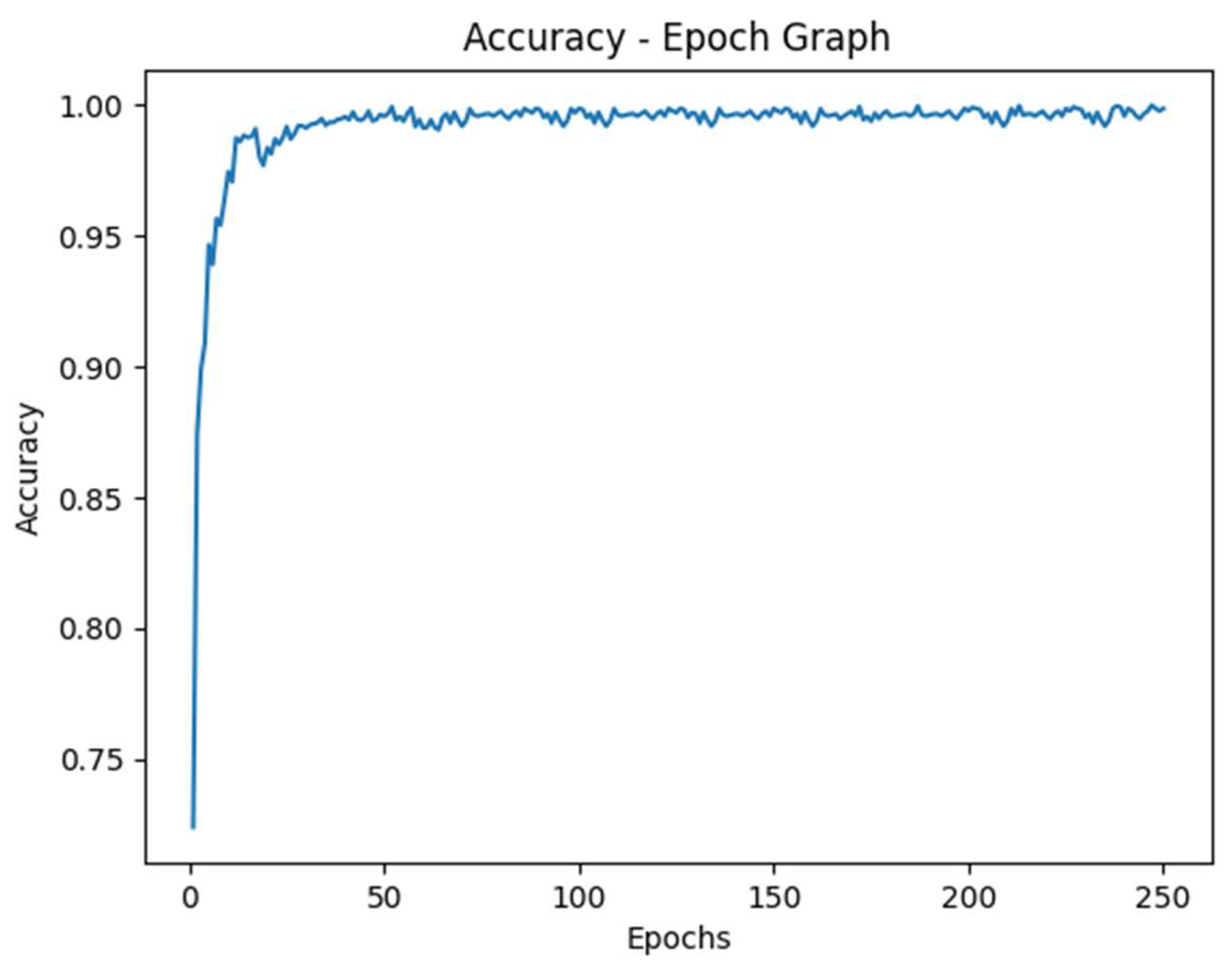
Figure 6. Loss vs Epoch Graph.

While the results are promising, there are some limitations that we should consider. The model’s performance, although tested against a huge and diverse dataset, might vary when applied to different populations or imaging technologies. Future research can lead to exploration of scalability of this approach across other types of cancers and medical imaging. Due to such high accuracy, there might be chances of overfitting, yet dropout layers are used to prevent the same. Lastly, integrating the model feedback into clinical trials and conducting extensive real-world testing is essential to assess the practicality and acceptance of such technology by healthcare professionals.

Conclusion

The study utilized powerful computational capabilities of the PARAM Utkarsh Supercomputer to develop a deep learning model for predicting kidney cancer from x-ray images, achieving an impressive peak accuracy of 99.8%. This research underscores the potential of supercomputing technology in revolutionizing medical diagnostics through advanced machine learning algorithms. The integration of technology in medical trials not only improves the accuracy and speed of disease detection but holds the promise to provide high-quality medical care and treatment. The successful application of the developed model in this study, to predict kidney cancer suggests a new pathway for similar advancements in other areas of medical imaging and disease diagnosis.

This study highlights the importance of interdisciplinary collaboration between computational and medical sciences. By bridging these domains, we can make use of the full potential of supercomputing resources to conquer complex health challenges more effectively. Future research should focus on expanding the applicability of such models to other diseases, integrating real-time diagnostic data, and improving the model’s adaptability to different clinical environments. Additionally, further validation through clinical trials and feedback from medical practitioners will be essential to refine the model and ensure its practical implementation in healthcare settings.

In conclusion, the findings of this study provide insights about the capabilities of supercomputers in medical diagnostics and makes the way for future innovations that could transform patient care on a global scale.

Acknowledgements

We would like to thank C-DAC Bangalore for allowing us to access computing resources of the PARAM Utkarsh Supercomputer throughout this study.

Statements and Declarations

The authors declare no conflicts of interests to disclose and have obtained necessary ethical clearances for our research. No external funding was received to conduct this study. The data that support the findings of this study are available upon request.

References

Vogelzang, N. J., & Stadler, W. M. (1998). Kidney cancer. The Lancet 352, 1691–1696. [CrossRef]
Chow, W.-H., Dong, L. M., & Devesa, S. S. (2010). Epidemiology and risk factors for kidney cancer. Nature Reviews Urology 2010, 7, 245–257. [CrossRef]
Ganti, S. , & Weiss, R. H. (2011). Urine metabolomics for kidney cancer detection and biomarker discovery. Urologic Oncology: Seminars and Original Investigations, 29(5), 551–557. [CrossRef]
Kim, K. , Aronov, P., Zakharkin, S. O., Anderson, D., Perroud, B., Thompson, I. M., & Weiss, R. H. (2008). Urine Metabolomics Analysis for Kidney Cancer Detection and Biomarker Discovery. Molecular & Cellular Proteomics, 8(3), 558–570. [CrossRef]
Kind, T., Tolstikov, V., Fiehn, O., & Weiss, R. H. (2007). A comprehensive urinary metabolomic approach for identifying kidney cancer. Analytical Biochemistry 363, 185–195. [CrossRef]
Morrissey, J. J., London, A. N., Luo, J., & Kharasch, E. D. (2010). Urinary Biomarkers for the Early Diagnosis of Kidney Cancer. Mayo Clinic Proceedings 2010, 85, 413–421. [CrossRef]
Kim, K. , Taylor, S. L., Ganti, S., Guo, L., Osier, M. V., & Weiss, R. H. (2011). Urine Metabolomic Analysis Identifies Potential Biomarkers and Pathogenic Pathways in Kidney Cancer. OMICS: A Journal of Integrative Biology, 15(5), 293–303. [CrossRef]
Tuncer, S. A., & Alkan, A. (2018). A decision support system for detection of the renal cell cancer in the kidney. Measurement. 2018, 123, 298–303. [CrossRef]
Hadjiyski, N. (2020). Kidney Cancer Staging: Deep Learning Neural Network Based Approach. 2020 International Conference on e-Health and Bioengineering (EHB). [CrossRef]
Da Cruz, L. B. , Araújo, J. D. L., Ferreira, J. L., Diniz, J. O. B., Silva, A. C., de Almeida, J. D. S., Gattass, M. (2020). Kidney segmentation from computed tomography images using deep neural network. Computers in Biology and Medicine, 103906. [CrossRef]
Kim, D.-Y. , & Park, J.-W. (2004). Computer-aided detection of kidney tumor on abdominal computed tomography scans. Acta Radiologica, 45(7), 791–795. [CrossRef]
Zhang, J., Lefkowitz, R. A., & Bach, A. (2007). Imaging of Kidney Cancer. Radiologic Clinics of North America 2007, 45(1), 119–147. [CrossRef]
Asha, V. , Sreeja, S. P., Prasad, A., Kathari, G. V., Karthik, A. S., Kathyayini, (2024). Classification of Images Related to Kidney Cancer using Hybrid Deep Learning. 2024 International Conference on Intelligent and Innovative Technologies in Computing, Electrical and Electronics (IITCEE). Bangalore, India. 1-6. [CrossRef]
Uhm, KH. , Jung, SW., Choi, M.H. et al. (2021). Deep learning for end-to-end kidney cancer diagnosis on multi-phase abdominal computed tomography. Npj Precision Oncology, 5(1). [CrossRef]
Türk, F. Türk, F., Lüy, M., & Barışçı, N. Machine Learning of Kidney Tumors and Diagnosis and Classification by Deep Learning Methods. International Journal of Engineering Research and Development 2019, 11(3), 802–812. [Google Scholar] [CrossRef]
Basandrai, A. et al. (2023). Medical Scan Classification Dataset (online) – Available at https://www.kaggle.com/datasets/arjunbasandrai/medical-scan-classification-dataset (accessed March 2023).
Center for Development of Advanced Computing. PARAM Utkarsh Supercomputer. https://paramutkarsh.cdac.in/.

Figure 1. Sample image of a cancerous kidney.

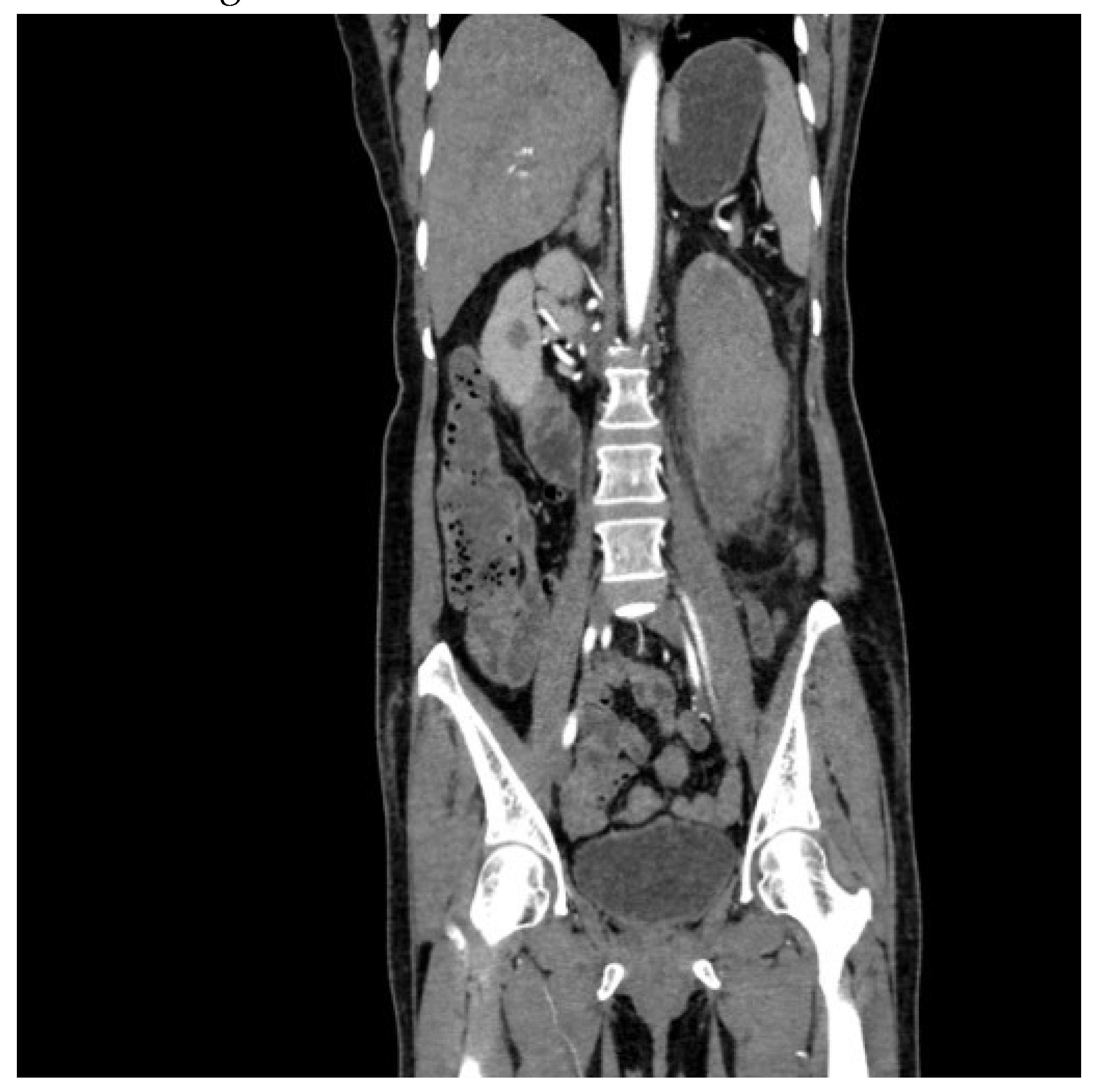
Figure 2. Sample image of a normal kidney.

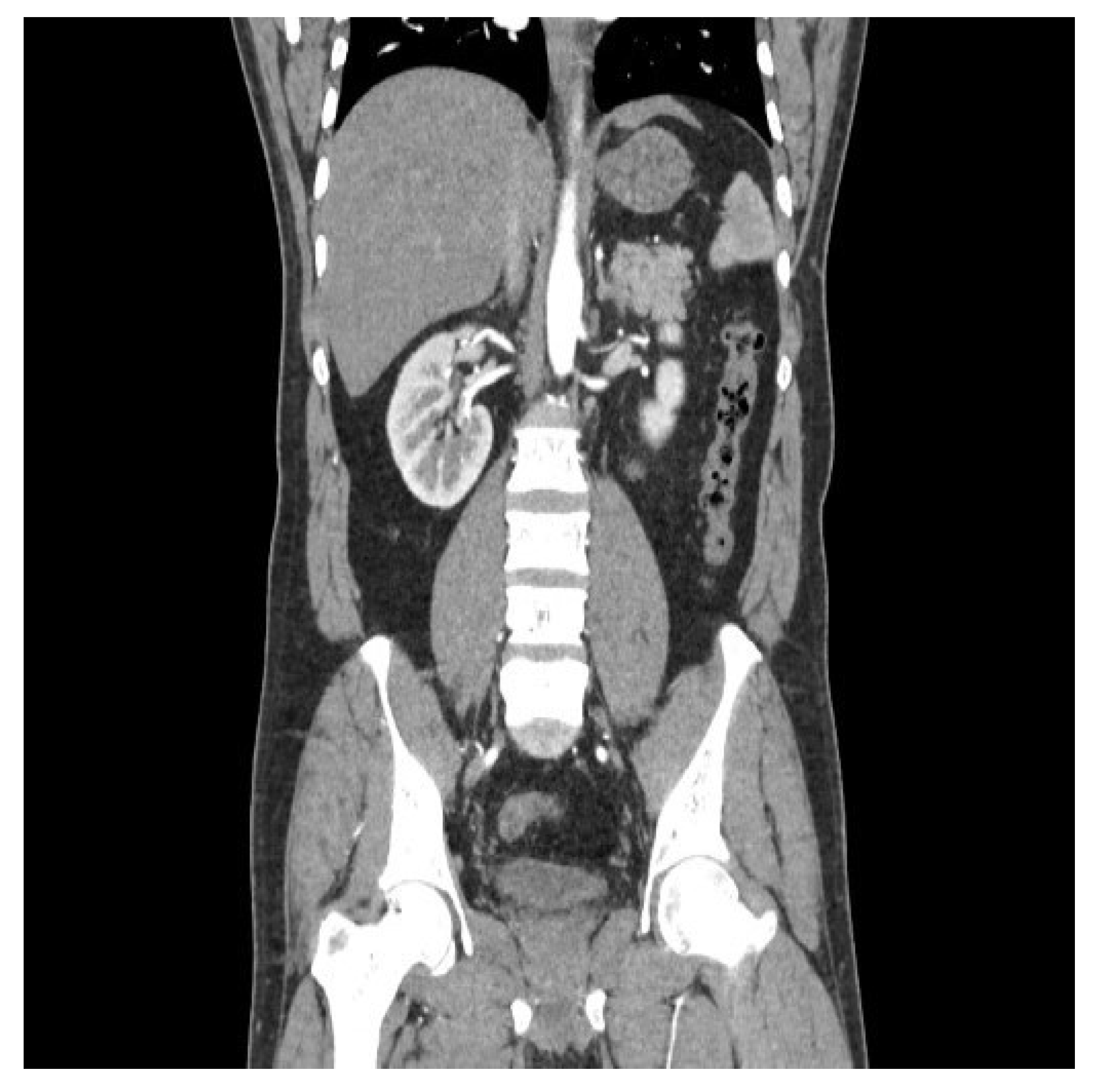
Figure 3. PreKiCan – Model flow.

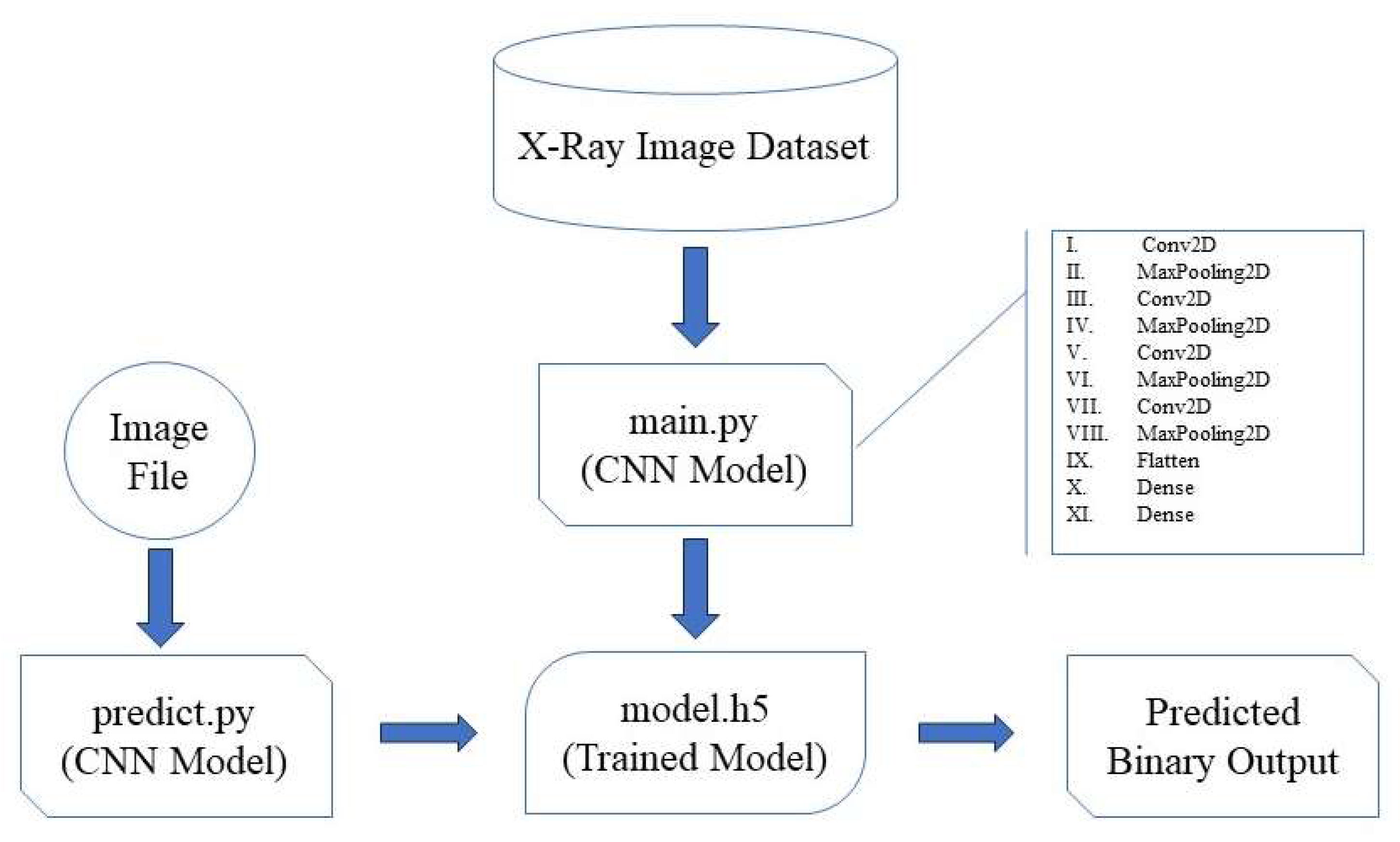
Figure 4. PreKiCan – Validation set Confusion Matrix: Output v/s Target.

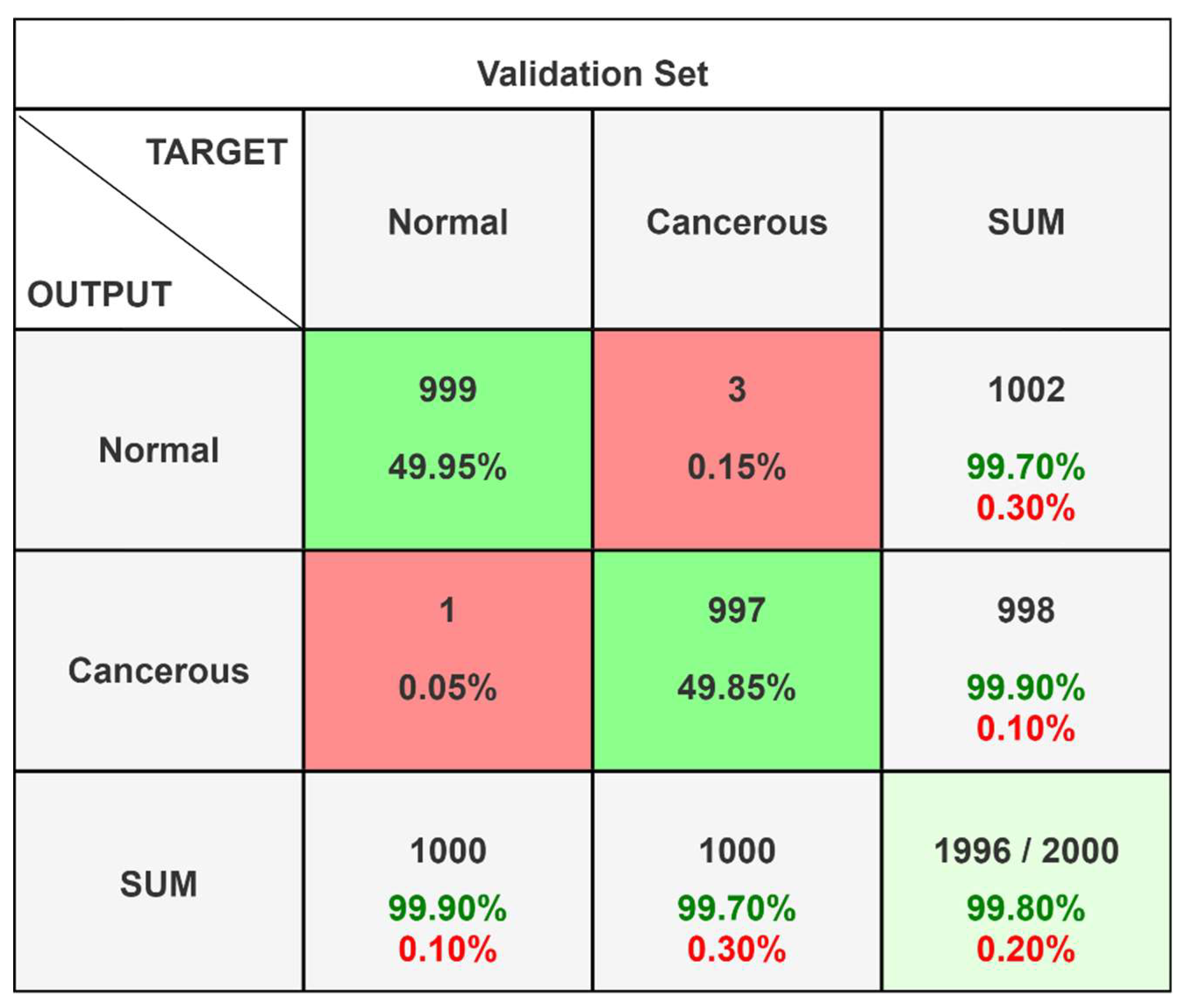
Table 4. PreKiCan - Classification Report.

Class Name	Precision	1-Precision	Recall	1-Recall	f1-score
Normal	0.997	0.003	0.999	0.001	0.998
Cancerous	0.999	0.001	0.997	0.003	0.998
Accuracy	0.998
Miss Rate	0.002

Disclaimer/Publisher’s Note: The statements, opinions and data contained in all publications are solely those of the individual author(s) and contributor(s) and not of MDPI and/or the editor(s). MDPI and/or the editor(s) disclaim responsibility for any injury to people or property resulting from any ideas, methods, instructions or products referred to in the content.

© 2024 by the authors. Licensee MDPI, Basel, Switzerland. This article is an open access article distributed under the terms and conditions of the Creative Commons Attribution (CC BY) license (http://creativecommons.org/licenses/by/4.0/).

Copyright: This open access article is published under a Creative Commons CC BY 4.0 license, which permit the free download, distribution, and reuse, provided that the author and preprint are cited in any reuse.