
Submitted:
06 November 2024
Posted:
07 November 2024
You are already at the latest version
Abstract
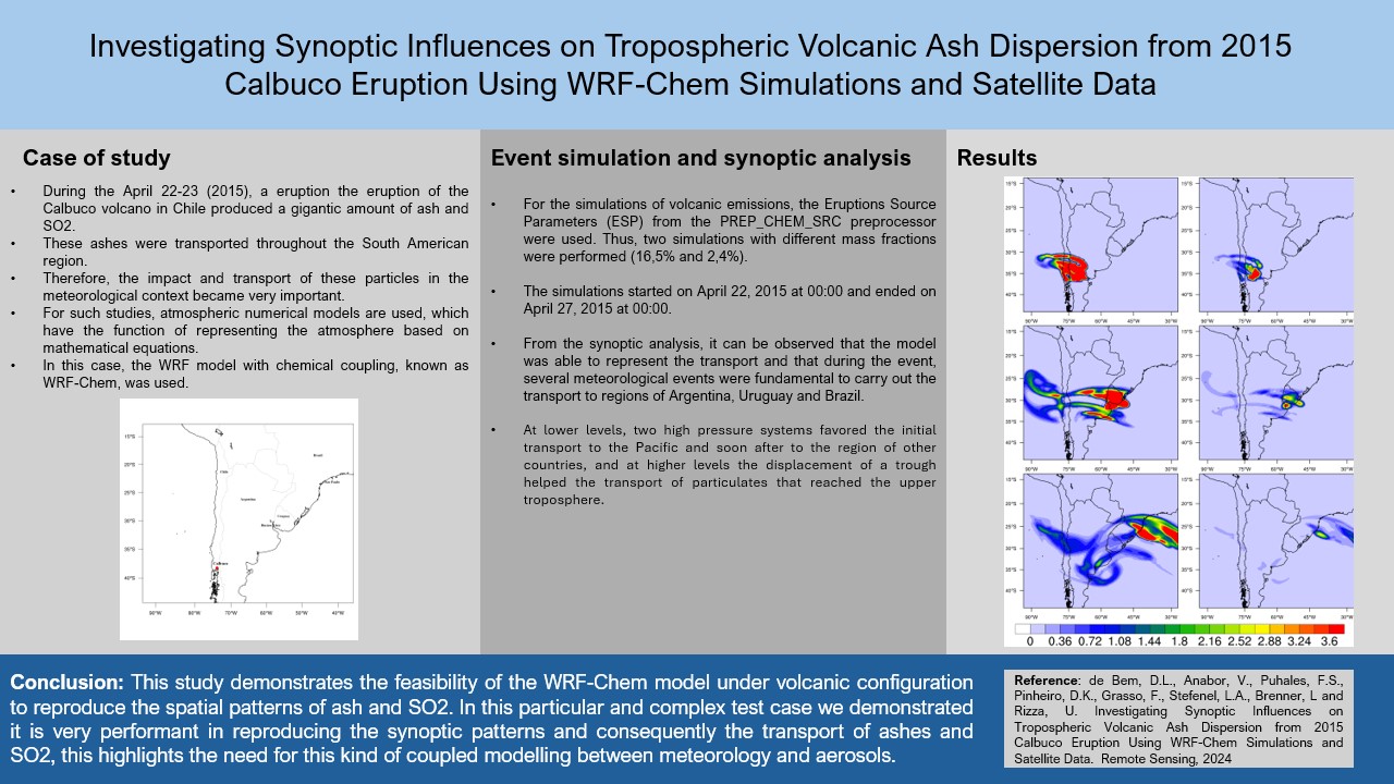
We used WRF-Chem to simulate ash transport from Chile’s Calbuco volcano eruptions on April 22 and 23, 2015. Massive ash and SO2 ejections reached the upper troposphere, and particulates were transported over South America, observed over Argentina, Uruguay, and Brazil via satellite and surface data. Simulations from April 22 to 27 covered eruptions and particle propagation. Chemical parameters utilized GOCART; meteorological conditions came from NCEP-FNL reanalysis. Two simulations (GCTS1 and GCTS2) differed in ash mass fraction in the finest bins (0–15.6 μm): 2.4% and 16.5%, respectively, to assess model efficiency in representing plume intensity and propagation. Analyzing active synoptic components revealed their impact on particle transport and the Andes’ role as a natural barrier. We evaluated and compared simulated aerosol optical depth (AOD) with VIIRS Deep Blue Level 3 data and SO2 data from Ozone Mapper and Profiler Suite (OMPS) limb profiler (LP), both sensors onboard the Suomi National Polar Partnership (NPP) spacecraft. The model successfully reproduced ash and SO2 transport, effectively representing influencing synoptic systems. Both simulations showed similar propagation patterns, with GCTS1 yielding better results. Comparison with VIIRS Brightness Temperature Difference data confirmed the model’s efficiency in representing particle transport. Overestimation of SO2 may stem from emission inputs. This study demonstrates WRF-Chem’s feasibility under volcanic configurations to reproduce ash and SO2 patterns enabling studies on aerosol-radiation and aerosol-cloud interactions and the understanding of atmospheric behavior following volcanic eruptions.
Keywords:
WRF-Chem
; Calbuco
; Ash
; Synoptics
; Aerosols
1. Introduction
Recent studies have shown the impact of ingesting aerosols into the atmosphere from volcanic eruptions on the Earth’s energy balance ([1,2]) along with their impact on cloud microphysics ([3]). Volcanic explosions inject volcanic ash, sulfur-bearing gases (mostly SO2), water vapor, CO2, halogens, N2, and other species into the lower stratosphere ([4]). According to Arghavani et al. [5] and Tsigaridis et al. [6], the annual emission of sulfur dioxide (SO2) can reach 9.2 Tg year−1 between natural and anthropogenic production. Even though anthropogenic production is five times higher than volcanic emissions, its effects are weaker due to the higher efficiency of volcanic sulfur in producing sulfate aerosols, which can be up to 4.5 times higher. This occurs because volcanic SO2 is emitted at high temperatures, reaching the stratosphere where it will have a longer residence time ([5]). As an example of direct impacts from the absorption of solar radiation by these aerosols, the eruptions of Mount Pinatubo in 1991 resulted in a global cooling of 0.5°C in the following years ([7]), while the Hunga Tonga eruption in 2015 produced an exceptionally large quantity of stratospheric aerosol, directly impacting the radiative balance ([8]).
Calbuco can be considered a major volcano in South America and its eruptions may have a considerable impact in the Andes area and in countries bordering the Chilean territory ([9]). Before 2015, 11 historical eruptions of Calbuco had been recorded since 1792, three of which had a Volcanic Explosivity Index (VEI; [10]) of order 3 or higher. The last major eruption in 1961 generated a volcanic plume approximately 12 km high and produced around 0.07 km3 dense rock equivalent (DRE) (about 0.2 km3 bulk), impacting the northeast sector of the volcano, including the city of Bariloche in Argentina ([11,12,13]). According to the report of the Chilean SERNAGEOMIN, during the month of April 2015, the volcano erupted again on the 22nd and 23rd, producing columns of debris and smoke that reached altitudes of 17 kilometers. Initially, the debris spread northwest of the volcano, and in the following days, it was carried across regions of Argentina, Uruguay, and Brazil.
The April 2015 Calbuco eruptions were investigated by Begue et al. [14], utilizing satellite data and lidar observations that highlighted the “Calbuco aerosol signal” on the Indian Ocean at Reunion Island one week after the first eruption (April 22), while JS Lopes et al. [15] investigated, with a suite of remote sensing data, the transport of volcanic ash in South America, indicating that the Calbuco volcanic aerosol layers could be classified as sulfates with some ash type. Van Eaton et al. [16] identified a new approach to quantify eruptive processes by combining lightning and umbrella expansion rates from the 2015 Calbuco eruption and suggested that ice formation above 10 km controlled the propagation of volcanic lightning downwind. For the same eruption, Romero et al. [17] presented a study analyzing the propagation of tephra—particulate material produced from a volcanic eruption—across the region near the event, using ground and satellite data. Marzano et al. [18], using various ground and satellite sensors, conducted a study on the propagation of volcanic ash and plumes, employing MODIS, VIIRS, CALIOP sensors among others, with a thorough investigation of particle size. They were able to demonstrate that the propagation of particulates occurred at higher atmospheric levels (between 15 and 20 km).
The numerical simulations of volcanic plumes have attracted increasing attention from the geophysics research community because of the deep impact of volcanic emissions on aviation and ground structures. Despite the understanding gained from remote sensing measurements, the numerical modeling of volcanic eruptions still remains an important scientific challenge. Some studies have aimed to represent the Calbuco 2015 eruption through the use of numerical modeling, such as Mastin and Van Eaton [19], who employed the Ash3d model ([20]) that considers an umbrella cloud model based on the calculation of downwind advection, turbulent diffusion, and particle settling. Such studies are of great importance for understanding the dynamics of the plume originating from the eruption and have already been conducted for other events, such as the Pinatubo (1991) and Kelud (2014) eruptions. However, these simulations fall short in representing the atmospheric processes and their active role in transporting particulates across the region. The eruption source parameters, such as the plume height, the mass eruption rate (MER), and the onset and end times of the paroxysm should be specified in a realistic way to obtain the forecast of ash column loading distributions for mapping flight hazard areas at the free troposphere levels ([21]). The WRF–Chem model has been previously applied to study the transport of ash and SO2 from volcanic eruptions all over the world. Stuefer et al. [22] made important progress on the WRF–Chem architecture, implementing specialized routines allowing the simulation of emissions, transport, and settling of volcanic particles and gases. Stenchikov et al. [23] recently applied the WRF-Chem model to study the radiative impact on the stratosphere caused by the Hunga eruption on January 15, 2022. They utilized a sophisticated approach using the sectional Model for Simulating Aerosol Interactions (MOSAIC; [24]). MOSAIC explicitly accounts for cloud–aerosol interactions, including aqueous chemistry and aerosol wet removal ([25]).
The region of higher latitudes in South America is directly impacted by the passage of meteorological systems known as transient systems ([26]). These systems function to transport air masses between the tropics and mid-latitudes. Marengo and Seluchi [27] indicated the orographic influence of the Andes Mountains on synoptic systems, thus acting as a barrier to the zonal flow in the Southern Hemisphere, with its greatest influence between 10° and 40°S. In this range, the westerly flow is completely blocked in the lower troposphere, channeling the meridional flow. Several studies indicate that this orographic influence favors the rapid northeastward propagation of transient systems crossing the Andes ([28,29]). Satyamurty et al. [30] used a numerical model to analyze the influence of the Andes, showing that the orography favors the intensification of lee cyclogenesis on the leeward side of the mountain. They are known as such due to their movement along the region, and their analysis is fundamental when discussing the transport of aerosols throughout the troposphere. The current literature still has gaps in the analysis of particulate transport during the event, specifically regarding which meteorological systems were crucial in carrying volcanic ash from a volcano in southern Chile to regions of Argentina and Brazil.
In this study, we make use of the WRF-Chem model to describe the two eruptions of the Calbuco volcano that occurred in April 2015, on the 22nd and 23rd respectively. From the meteorological perspective, we analyze the transport of tropospheric volcanic ashes in South America and their relationship with the synoptic system. From a general point of view, the impact of the Calbuco eruption has been largely documented by different techniques and different authors, but there are few studies that use this event to test the WRF-Chem model under the volcanic configuration, and this approach is important for studies that require an integrated approach between meteorology and aerosols and their mutual feedbacks.
To perform a comprehensive validation, we first analyze the synoptic patterns during and after the eruptions by analyzing the satellite products of the VIIRS sensor at visible (AOD) and thermal IR (BTD) channels, then we compare the simulated data with the AERDB_D3_VIIRS_SNPP and with the SO2 concentration from the sensor OMPS (Ozone Mapping and Profiler Suite), which is also onboard the SUOMI-NPP spacecraft.
2. Materials and Methods
2.1. Description of the Event
Detailed descriptions of what happened during the April 22–23 (2015) eruption of Calbuco, Chile, are reported by Romero et al. [17], Van Eaton et al. [16], and Marzano et al. [18], among others. The first eruption started at 21:05 (UTC) on April 22; the ash column rose to 16 km and ejected approximately 40 million cubic meters of ash in about 90 minutes ([16,17]). The second eruption began at 04:00 UTC on April 23, with an ash column reaching 17 km, and ejected around 170 million cubic meters of ash over 6 hours (see Table 11,2) ([16,17]). The magma involved in the eruption was a typical ESP S-type eruption with andesite/dacite, containing volcanic glass and crystals of plagioclase and amphibole, with minor quartz and biotite ([17]). The SO2 gas release from the eruption was substantial—around 0.2–0.4 million tons—but probably some way short of the levels needed to have a significant impact on the climate system ([14,31]).

Table 1.
Eruption parameters (SERNAGEOMIN).
| Start Time | Durantion | emiss height | emiss ash rate | emiss SO2 |
| UTC | min | km | kg s-1 | kg h-1 |
| 22/04/2015 - 21:00 | 90 | 16 | ||
| 23/04/2015 - 04:00 | 360 | 17 |
2.2. Synoptic Analysis During the Event
Usually, synoptic systems evolve over a timescale of a couple of days, so time frames between 12–24 hours are sufficient to represent the evolution of atmospheric processes at this timescale. The first Calbuco eruption started at 21:00 UTC on April 22, 2015, and a few hours later, at 00:00 UTC on April 23, 2015, a transient elongated anticyclonic high-pressure system (High) was located over the Pacific Ocean along the Southern Chilean coastal range at low levels, between latitudes 30°S and 45°S (Figure 1c). This high ridge extended over the eruption area in a thermally homogeneous and weak pressure gradient environment, creating a statically stable and low wind shear environment in the lower troposphere. This scenario provided the dynamic and thermodynamic conditions for the Calbuco eruption plume to rise vertically and rapidly reach the stratosphere. The geopotential height field at 500 hPa showed a long wave pattern extending from the Pacific to the Atlantic Ocean below 40°S (Figure 1d), just south of the eruption area where the geostrophic flow was mainly westward, accelerating the erupted mass portion across the Andes towards Argentina at this level. In the middle troposphere, a Cut-off Low (COL) pressure system was forming ahead and detaching from a midlatitude shortwave in the westerlies that was amplifying from the Buenos Aires region towards the Pacific Ocean (30°S, 90°W) ([32,33]). This COL system would play an important role in the following hours by trapping a portion of particulate material and gases from the eruption on the west side of the Andes. At upper levels of the troposphere, the eruption area was upstream of a long wave trough in which the Polar upper-level jet was embedded (Figure 1b). An amplifying shortwave was located over the COL, as observed in the 200 hPa wind field. South of the eruption area, a diffluent flow split from the polar jet towards the subtropical jet entrance region, forming a northward flow on the lee side of the Andes (Figure 1b). This caused the first volcanic plume to be advected and spread northward. The position between the subtropical and polar upper-level jets was still far from their vertical motion influence perimeters, being in a favorable to neutral region for vertical motions relative to the 200 hPa wind field ([34,35]). At levels close to the surface, the influence of the high-pressure system in the Pacific could be observed, with its anticyclonic circulation helping the winds transport the plume towards the northwest, possibly crossing the Andes Mountains (Figures 1a,1c). During the next day after the first eruption, synoptic conditions favored a higher concentration of the plume in the region near the volcano, with upward movement promoting the vertical propagation of this plume. At lower levels, the circulation favors transport towards the Pacific, while at higher levels, stability favors the concentration of the plume over the region.
In the first hours of April 24, 2015, the low levels of atmospheric features presented almost the same conditions, keeping the favorable conditions for the thermal volcanic plume ascent vertically in a low wind shear environment (Figure 2a). The sea-level pressure field corroborates the previously indicated information (Figure 1c), while the high-pressure system acting over the regions of Argentina, Uruguay, and Brazil favors the transport of particulates towards Uruguay and southern Brazil. However, at 500 hPa the geopotential horizontal gradient is stronger, denoting an intensification of the eastward geostrophic advection by geostrophic wind at this level (Figure 2d). The 500 hPa amplified shortwave formed a COL upstream in the Andes and a high-level cyclonic vortex (HCV) over South Brazil; both systems act as convergence centers. The COL keeps a small portion of the plume east side of the Andes, and the HCV pulls the plume to low latitudes. The polar upper-level jet streak at 200 hPa is displaced eastward (Figure 2b); by this time the Calbuco area is at the equatorial entrance of the polar upper-level jet streak, a region favorable for upward vertical motion ([35]). The subtropical jet stream also moves eastward over South Brazil and acts as a kinetic barrier preventing the plume from reaching São Paulo, the most populated city and the most important commercial aviation center in South America. The mean upper-level flow between the jet streaks drives the plume east equatorward to be SW-NE oriented (Figure 2b). During the second day of the event, the transport of particulates (both at lower and upper levels of the troposphere) is directed over the regions of Argentina, Uruguay, and Brazil; this is caused by the direct influence of synoptic systems, such as the two high-pressure systems along with the shortwave seen at 500 hPa moving over the region.
Two days after the last volcanic eruption, April 25, 2015, areas with high concentrations of volcanic gases and aerosol particles ([16,31,36]) are still present in the upper troposphere. Weak thickness and pressure gradients at mid-latitudes all over South America indicate a low wind speed and thermally homogeneous environment (Figures 3a,3c); at this moment the volcanic plume is mostly concentrated at the high levels of the troposphere. At 500 hPa, the systems COL and HCV have intensified and are deeper than the previous day; a cyclonic vorticity channel connects both systems (Figure 3d). The upper flow at 200 hPa (Figure 3b) presents a short ridge over southern Argentina and a short trough over southern Brazil and denotes the high influence of the upper-level flow spreading the volcanic plume. The subtropical jet stream entrance region is over Southern Brazil, and the 200 hPa streamlines present a high confluence in the region that increases the local plume concentration (Figure 3b). The propagation of the wave seen in the geopotential and relative vorticity fields (Figure 3d) allows the transport of the plume in the upper troposphere to regions of lower latitudes, potentially reaching southeastern Brazil. By the end of the third day of the event, the plume’s propagation in the upper troposphere can be observed reaching the southeastern region of Brazil. Meanwhile, at lower levels, due to the stability generated by the high-pressure system and its circulation, the highest concentration of the plume remains around the region between the three countries, as seen on the 24th.
On April 26, 2015, the upper-level systems evolved eastward and the high confluent area at the entrance of the subtropical jet was displaced over São Paulo and advected the plume over the city (Figure 4b). The active trough moving over the region also played an important role in the transport of the plume at upper levels (Figure 4d). As the local and synoptic effects diminished their influence in the days following the eruption, the plume was transported as indicated above to the southeast region of Brazil, thereby reducing its concentration over the event area. During this eruption, the Subtropical Jet Stream and the Polar Jet Stream acted as kinetic barriers to the plume advection, and the momentum transference between them determined the plume advection ([29,35]). At lower levels, the movement of the high-pressure system located over the southern region of Brazil (Figure 4c) favors the transport of the plume over the region throughout the day due to its circulation (Figure 4a), resulting in greater dispersion compared to the previous day. During the period following the volcanic eruption, the direct impact of synoptic conditions on plume transport over the region can be observed ([26,28]). At lower levels, high-pressure systems initially favored transport towards the Pacific on the first day, and subsequently, the formation of another high-pressure system over the region between Argentina and Brazil favored transport towards lower latitudes. At upper levels, it can be seen that due to an initial southwesterly circulation at 200 hPa, the vertical development was more intense, helping the plume reach higher altitudes, even reaching the stratosphere ([18]). With the trough’s movement during the 24th and 25th, this plume, which had reached upper levels, was transported over the southern regions of Brazil, Uruguay, and central Argentina. With the development of all these synoptic systems, the plume managed to be transported over the region.
2.3. Orography Influence
The Andes Cordillera, the largest and tallest mountain range in the Southern Hemisphere, runs continuously along the Pacific coast of South America, having a direct impact on the passage of meteorological systems and synoptic fields. For studies on the transport of aerosol particulates, it is of utmost importance to understand the wind field alongside topographic analysis. Such topographic analysis indicates that circulations associated with topography are crucial for defining air trajectories, which are necessary for assessing the impact of atmospheric pollution. Additionally, it is known that regions with complex topography can have direct impacts on large-scale movements ([37]). Another study by Seluchi et al. [29] highlights the blocking effect generated by the mountain range along the zonal flow at lower levels. The mountain range, due to its height, acts to prevent the spread of easterly winds, thereby intensifying upward movement, impacting not only the zonal flow but also the thermal field over the South American region. Based on the analysis of observed data during the volcano eruption, the mountain range may have acted as a barrier to the eastward transport of ash particles, while also favoring upward flow, suggesting its propagation along the stratosphere. An important point to highlight is that if the natural barrier were not present, the dispersion of particulates, such as those from the Calbuco volcano, would be observed in a more distributed manner, that is, being seen in all directions, similar to what can be observed with some volcanoes located on islands, such as the Hunga Tonga volcano ([8]).
2.4. WRF-Chem Model: Setup for Volcanic Emissions
It has recently included a new functionality inside the Weather Research and Forecasting (WRF) with Chemistry (WRF-Chem, [38]) model that allows simulating the emission, transport, transformation, and settling of aerosols and gases released during volcanic eruptions ([22]). Many specialized options are available for the treatment of volcanic ashes and gas (SO2), among the most common we mention: (i) the invariant tracer using four ash variables and no chemistry modules (chem_opt = 401), (ii) the intermediate options using ten ash variables and SO2 (chem_opt = 402), and (iii) a more sophisticated approach that utilizes the GOCART-SIMPLE option (chem_opt = 300) with all the optical drivers activated ([39]). As reported in Table 1, the Eruption Source Parameters (ESP) define the plume altitude, the mass of the eruption cloud, and the particle size distributions. It is important to mention that Mastin et al. [40] have developed ESP for all the world’s volcanoes with a “typical” eruption profile assigned to it. In this context, all the possible eruption categories may be classified as M-type, or mafic types, which include basaltic and ultramafic magmas; and S-type, or silicic types, which include andesite, dacite, rhyolite, and others such as phonolite that can produce high ash columns ([40], Tables 3 and 4).
Table 2 gives the selected particle size bins, which have been associated with the WRF-Chem variable names vash_1 to vash_10, and the corresponding mass fraction percentage for each volcano S-type distribution. The mass fraction has been configured by Steensen et al. [41] and Stuefer et al. [22] considering previous works from Scollo et al. [42] and Rose and Durant [43] among others. To select the appropriate ESP during a specific volcanic eruption event, it is possible to use the emission preprocessor package PREP_CHEM_SRC ([44]), which has incorporated the full database developed by Mastin et al. [40] (M09). In this context, there is information on 1535 volcanoes around the world, comprising location (latitude, longitude, and height) as well as the corresponding historical ESP ([22]). The default configuration for Calbuco considers an ESP of type S2, with (lat, lon) coordinates and an elevation of 2003 meters. Moreover, the preprocessor provides the proper localization of the selected volcano in the domain grid. This is reported in the following Figure 5.
The numerical grid has (150,130) grid points with geog_data_res = ’30s’, and (dx, dy) = (30, 30) km upon a polar map projection. The simulation started at “2015-04-22_00:00:00” and stopped at “2015-04-27_00:00:00”. The initial (ICs) and boundary conditions (BCs) are provided by NCEP-FNL (Final) operational global analysis/forecast fields at 0.25° spatial resolution ([45]). In WRF-Chem, emissions units for volcanic ash rate (E_VASH) are µg m−2 s−1 and for SO2 (E_VSO2) are mol h−1 km−2. In Table 1, the total erupted mass is calculated using the corresponding erupted volume times the ash mass density, which is defined as being 2,500 kg m−3. The total emission ash rate is then distributed following a typical “umbrella” plume model ([46]) between 10 bins of aerosol particles with a diameter size range reported in Table 2 ([22]). Note that the default ESP parameters for a given volcano/eruption may be overwritten in the WRF-Chem emission driver Fortran routine. This was done by changing manually the specialized subroutine for the volcanic emission; in our version of the WRF-Chem code, it is allowed a multi-eruption for a single run, as in the current case (see Table 1). Regarding the model setting of the physical parameters, the surface layer module corresponds to the MYNN ([47,48]) scheme (sf_sfclay_physics = 5), the RUC (Rapid Update Cycle) Land Surface Model ([49]) is used to represent the land surface interactions (sf_surface_physics = 3), and the Mellor–Yamada–Nakanishi and Niino (MYNN) 2.5 level ([50]) turbulent kinetic energy parameterization is used to describe the PBL parameterization (bl_pbl_physics = 5). Short and long-wave radiation effects are modeled using the Rapid Radiative Transfer Model for both short- and long-wave (ra_sw_physics = ra_lw_physics = 4); the two-moment cloud model microphysics scheme of Morrison et al. [51,52] is used for the treatment of the microphysical processes (mp_physics = 10). The chemistry/aerosol setting is depicted in Table 3; the use of chem_opt = 300, that is, the GOCART aerosol model, activates the WRF-Chem optical modules. Aerosol optical properties are derived using the Maxwell-Garnett volume averaging mixing rule (aer_op_opt = 1), which allows the calculation of the extinction coefficients from which AOD may be calculated. For this aerosol option, the finest three ash bins (vash_8, vash_9, and vash_10) are combined into a “p10” variable, which is generically defined as unspeciated aerosols in the WRF-Chem registry configuration. This option also allows the capability of considering the feedback of volcanic ash with the radiation and the microphysics ([22]). Two simulations have been considered: the first one, GCTS2, utilizes the ash granulometry expressed by the S2 distribution reported in Table 2; the second one, GCTS1, is configured with S1 ash distribution. The difference between the two is the percent of mass fraction in vash_8–vash_10, which is 2.4% for S1 and 16% for S2. In this condition, the GCTS1 simulation has a lower content of the finest ash.
Table 3.
Volcanic setup of the WRF-Chem model.
| case | chem_opt | distribution | vash_ # | % total mass |
| GCTS2 | 300 | S2 | 8-10 | 16.5 |
| GCTS1 | 300 | S1 | 8-10 | 2.4 |
2.5. Description of the Event by AOD from AERDB OMPS-SNPP
The level-3 (L3) Deep Blue ([53]) daily aerosol products from the Suomi National Polar-orbiting Partnership (SNPP) spacecraft provide satellite-derived measurements of Aerosol Optical Depth (AOD) and their properties over land and ocean as daily gridded aggregates. The Deep Blue algorithm was initially developed to fill gaps in the aerosol optical depth (AOD) retrievals over some bright surfaces such as deserts and urban areas, where existing ‘dark target’ (DT; [54]) approaches based on dense dark vegetation assumptions fail. Since 2012, it has been complemented with the Satellite Ocean Aerosol Retrieval (SOAR; [55]) algorithm to provide aerosol data coverage over the ocean. Later, a second-generation approach was developed ([53]) which extended Deep Blue’s coverage to darker surfaces. In this context, the AERDB/AOD provides coverage, in principle, for all snow-free, cloud-free land surfaces. This daily aggregated product (Short-name: AERDB_D3_VIIRS_SNPP3), that is utilized in this study, is derived from the Version-2.0 (V2.0) L2 6-minute swath-based products (AERDB_L2_VIIRS_SNPP), and is provided in a 1° x 1° degree horizontal resolution grid. This Level 3 daily product (in netCDF format) contains 45 Science Data Set (SDS) layers that include the "aerosol optical thickness estimated at 550 nm over land and ocean". It is represented in Figure 6, in which it is reported the daily average AOD from AERDB (SNPP-D3-VIIRS) for (a) April 23; (b) April 24; (c) April 25; (d) April 26. It can be observed from this AOD product that on April 23 there were high AOD values (greater than 1.5) in a region at around 300 km from the volcano (Figure 6a); this indicates the absence of an efficient atmospheric transportation system of these ash particulates. This is due to what was discussed and presented in figures Figure 1a and Figure 1c, where the high-pressure system and its anticyclonic circulation at low levels promote weaker transportation due to its winds towards the northwest region and the Pacific. Meanwhile, the Andes’ natural barrier favored vertical penetration, maintaining a higher concentration over the region and transporting these particulates to the upper troposphere and stratosphere. The statically stable environment and low wind shear in the lower troposphere favored the uplift over the region, leading to a higher concentration of ash particulates during the day of the 23rd, with low dispersion. On the following day (April 24), the ash plume is further transported northeast toward the city of Buenos Aires and southern Uruguay (Figure 6b), due to the displacement of the upper-level trough (Figure 2d). On the 25th, the conditions at low levels are similar to the previous days; however, the upper levels of the atmosphere are crucial for the dispersion of particles toward the regions of Argentina and Brazil (Figure 6c). This is due to the horizontal geopotential gradient at 500 hPa in Figure 3d, which favors a geostrophic advection eastward. The cyclonic vortex at high levels and the COL acting as centers of convergence facilitate the transport, aiding the plume to be displaced to lower latitudes. At 850 hPa, the anticyclonic circulation acting over the region of Argentina throughout the day on the 24th favors the displacement of the plume towards the region of Uruguay, as seen in Figure 3a. On April 25 and 26 (Figure 6c, Figure 6d), the plume was directed into the Atlantic along the coastline of southern Brazil. The upper-level systems evolved eastward, and the area of high confluence at the entrance of the subtropical jet was displaced over São Paulo, advecting the plume over the city. As seen in the synoptic analysis, the Subtropical Jet Stream and the Polar Jet Stream played a fundamental role in the concentration and transport of the eruption plume due to their function as a kinematic barrier for the advection of the plume and the momentum transfer between them ([29,35]).
2.6. Description of the Event by the Split Windows Imagery by VIIRS
The use of the Brightness Temperature Difference (BTD) of the thermal infrared channels to track volcanic ash may be dated back to Prata [56]. It is based on the reverse absorption effect (in the infrared window) observed for volcanic debris that provides a signature that may be utilized to discriminate volcanic clouds from water/ice clouds ([56]). Figure 7 shows the BTD of the VIIRS thermal infrared M-channels (700 m spatial resolution). It was calculated following the Split Window Volcanic Ash Detection Method that consists of calculating the difference between channels M15 (10.763 m) and M16 (12.013 m) of the VIIRS sensor:
As depicted in Table 4, the SUOMI spacecraft had useful orbits in South America for the selected days, making it possible to draw the BTD map that is shown in Figure 7. The blue shaded regions in Figure 7 highlight the presence of ash plumes with BTD ; on the contrary, ice and water droplet clouds (yellow-red shaded) are denoted by regions with BTD .
A qualitative agreement may be found with the AOD maps reported in Figure 6. Starting from April 23 (Figure 7a) until April 26 (Figure 7d). In the four panels of Figure 7 the position of the ash cloud is denoted by the blue shading region confirming the transport of the ash plume as seen in the previous paragraph about the synoptic pattern. This analysis, based on IR channels, together with the analysis of AOD at 0.55 m , provides a definitive picture of ash transport in South America after the April 22 and 23 Calbuco eruptions.
3. Results and Discussion
3.1. Comparison with Satellite Data
3.1.1. AERDB_D3_VIIRS
Considering the WRF-Chem setup reported in Table 3, it is important to remark that the calculation of aerosol optical properties, among the large number of chemistry packages actually available in WRF-Chem distribution, is possible with chem_opt = 300 (GOCART_SIMPLE configuration). This may be very useful as it allows us to discriminate which one of the S1 and S2 grain distributions is more appropriate for this particular case study (Table 2). This may be done by comparing the Aerosol Optical Depth (AOD) from the model output with the AERDB/AOD retrievals ([53]) described in paragraph 2.3. The GOCART aerosol model activates the WRF-Chem optical modules, which allows the calculation of the plume optical properties, like the extinction coefficients at 0.55 m (extcof55), from which the AOD may be calculated offline as follows:
where the integration is performed from the bottom vertical level () up to the upper top level () and is the depth of the layer between levels i and . Our analysis starts by comparing the daily averaged AERDB ([53]) (Figure 6) products for the AOD at 0.55 m with the corresponding simulated quantity calculated with Eq. 1. In Figure 8, we report the numerical AOD obtained for GCTS2 (left column) and GCTS1 (right column) configurations (see Table 3). The first row (panels a,b) is calculated at 19:00 UTC on April 23; the second row (panels c,d) is calculated at 19:00 UTC on April 24; and finally, the third row (panels e,f) is calculated at 19:00 UTC on April 25. What is immediately evident is (i) the overestimation of AOD by the GCTS2 simulation; and (ii) the good reproduction of peak values and the spatial pattern of AERDB/AOD by the GCTS1 simulation. This is evident by comparing Figure 8b with Figure 6a for April 23 and Figure 8d with Figure 6b for April 24. This means that the S2 total grain distribution produces a considerable overestimation of the quantity of ash in the numerical domain, while the GCTS1 setup and the associated S1 grain distribution, even if still overestimating, appears to be more appropriate for this situation. To analyze each day separately, we have complemented Figure 8 with Figure A1:A5 reported in Appendix A. This helps in the analysis of different vertical layers and specifically, it may explain the role of the synoptic systems in the propagation of the ash clouds. On April 23, at 19:00 UTC, model AOD is depicted in Figure 8b (GCTS1 run). It is evident the very good reproduction of experimental AERDB/AOD ([53]; Figure 6a), in terms of spatial pattern and intensity. Figure A1,A2 suggest that most of the p10 ash content is in the upper levels (17–20 km), corroborating the effect of plume lifting induced by the Andes Mountains. At lower levels, the ash plume is spread toward the Pacific Ocean by the high pressure located along the continent’s coast, which favors southwest transport, allowing it to cross the Andes. As indicated, the highest concentration of particulates was transported to higher levels due to a greater influence of vertical movement caused by the orography on the 23rd. By the end of the day, the increase in the intensity of easterly winds to the south of the eruption region favored the transport at lower levels towards Argentina. On April 24, the GCTS1 model prediction is depicted in Figure 8d. It may be noticed that the plume has traveled for more than 2000 km in the northeast direction, reaching Uruguay and the city of Buenos Aires. This is also reported by AERDB/AOD ([53]; Figure 6b) and BTD (Figure 7b). The propagation of the plume corroborates the eastward transport in the upper troposphere as seen in Figure 2d. Additionally, at lower levels, the eastward anticyclonic circulation indicates transport at lower levels to regions of Argentina, Uruguay, and Brazil (Figure A2). The highest concentration is observed at high levels due to the vertical movement on the 23rd, which intensely transported these particulates to higher levels. In the Pacific region, due to the stability generated by high pressure along the continent’s coast, the maintenance of transported AOD is observed throughout the 23rd. The maps for April 25 are reported in Figure 8f and Figure A3. It is noteworthy to highlight the further displacement of the volcanic plume in the northeast direction, towards the Atlantic coasts of Argentina, Uruguay, and southern Brazil. This is caused by the displacement of the trough in the upper troposphere (Figure 3d), effectively transporting these particulates and indicating from the simulations that the plume reached densely populated regions of Brazil such as São Paulo and Rio de Janeiro. At lower levels, combined with the high-pressure system in the region, the formation of a low-pressure system favors the confluence of easterly winds, intensifying the winds. However, due to the high pressure, the particulates remain over the region encompassing the three previously mentioned countries (Figure A3).
In the following days, the volcanic plume moved in the direction of the African continent (not shown) that was reached at the end of April 2015 ([14]). The data presented from the average AOD representation in the GCTS1 setup corroborates with what was observed both in the BTD (Section 2.4) and the AOD values from VIIRS (Section 2.3), where the first day of the event shows a higher concentration of particulates in the region near the volcano, with effective transport to higher levels of the atmosphere. On the second day post-eruption, meteorological events at both upper and lower levels directly impact the transport and concentration of the particulates, indicating the displacement to the regions of Argentina and Uruguay in higher concentration. During the 25th, the influence of a trough transports these particulates over the southeastern region of Brazil at high levels, while the high pressure at lower levels favors the maintenance of these particulates, in lower concentration, over central Argentina. Even at a reasonably higher concentration, the GCTS2 also manages to represent the transport of these particulates, indicating that the model successfully represented the meteorological systems acting over the region during the event. The conclusion that may be drawn from these results is that the optical properties are better reproduced by the GCTS1 setup; this means that, in terms of the S-type granule range, the S1 distribution with a lower mass of fine-size particles is better suited for simulating the transport of the Calbuco volcanic plume.
3.1.2. OMI/OMPS
The Ozone Mapper and Profiler Suite (OMPS) limb profiler (LP) onboard the Suomi National Polar Partnership (NPP) spacecraft provided the best plume coverage for the Calbuco eruption in April 2015 and estimates the SO2 emission of 0.2 Tg in its first overpasses following the eruption. On the web page of the Atmospheric Chemistry and Dynamics Laboratory of the Goddard Space Flight Center (NASA), it is possible to download Sulfur Dioxide Images Galleries for a large set of world volcanoes in the time period 2011 to present. In particular, concerning the Calbuco April 2015 eruption, there are reported high-resolution composites of Ozone Monitoring Instrument (OMI onboard Aura spacecraft) and OMPS images. The emission of SO2 is estimated by the SERNAGEOMIN (Chilean Geology Service) to be kg h−1 for the first eruption and kg h−1 for the second one (Table 1). This may be a critical point; these estimations should be replaced by direct measurements with some remote sensing technique to provide a realistic time-varying emission rate of SO2 ([21]). To check the quality of WRF-Chem simulation of the transport of SO2 in South America, we compared model outputs with satellite retrievals. The composite OMI+OMPS SO2 retrievals for April 23 are depicted in Figure 9a; the columnar SO2 distribution after the two main eruptions is dislocated from the Pacific Ocean (5 DU) to internal Argentina with a concentration of the order of 20 DU and peak value of 47.35 DU at longitude 71.38°W and latitude 36.55°S. WRF-Chem model output reported in Figure 9b reproduces (i) the spatial pattern with a little overestimation and (ii) the position and intensity of the peak value.
As discussed in previous sections, on April 24 the SO2 volcanic plume was transported toward Uruguay and the city of Buenos Aires with maximum values around 40 DU. A long tail reached the Ocean Pacific with a concentration of the order of 10 DU. The comparison between the model (fig.10b) and satellite retrievals (fig.10a) revealed an optimal comparison for the spatial pattern and concentration of the columnar SO2.
Two days after the first eruption, April 25, the SO2 plume moved further in the north-east direction with the largest part in the offshore coasts of southern Brazil (fig.11a) with more than 15 DU. Again, the WRF-Chem predictions are in good agreement with experimental data (fig.11b) if considering the spatial distribution and the columnar concentration with a maximum in the range of 15-20 DU.
Finally, on April 26 the SO2 plume moved offshore in the direction of the African continent and reached the Indian Ocean one week after the first eruption ([14]). The comparison between the SO2 dispersion maps simulated by the model, and data observed by OMI-OMPS show fair agreement but with a little overestimation of the simulated concentration of SO2. This may be caused by the overestimation of the SO2 experimental emission rate.
4. Conclusions
In this study, we used the WRF-Chem model ([38]) to describe two eruptions of the Calbuco volcano that occurred on April 22 and 23, 2015. The model configuration under the GOCART speciation for aerosol ([39]) allows us to activate the optical modules from which it is possible to calculate (offline) the model AOD that can be compared with satellite retrievals, AERDB_D3_VIIRS_SNPP in this case. Two different distributions of the ash granulometry from the WRF-Chem database ([22]) are tested against experimental satellite data to find the best option for Calbuco. To our knowledge, this study represents the first application of the WRF-Chem package to model eruptions from Calbuco. The transport of ash in the numerical domain has been analyzed in terms of synoptic meteorological conditions that are peculiar for the South American continent and evidenced the role of the Andes Mountain range in lifting the ash plume to the high troposphere and the blocking of zonal winds ([27,37]). In this context, the synoptic characterization during the simulated period from April 22–26 can be divided into lower and upper levels. It is verified that due to the more intense ejection during the second eruption, the plume managed to reach higher levels of the atmosphere ([17]). In addition, the southwestward wind at high levels favored the intensification of vertical movement, helping the plume to reach the upper troposphere. In the following days, the displacement of a trough over the regions of Argentina, Uruguay, and Brazil assisted in the propagation of this plume ([29]). When observing the lower portion of the atmosphere, the presence of a high-pressure system offshore the Chilean coast caused the transport of ash toward the Pacific Ocean during the first day. In the following days, the influence of a high-pressure system forming over the northern region of Argentina favored the propagation of the plume over the central region, reaching the cities of Buenos Aires and Montevideo. On the 25th, the confluence of eastward winds due to the emergence of a low-pressure system to the south of the continent intensified transport over the northern regions of Uruguay and southern Brazil. Therefore, based on the analysis, the WRF model successfully represented these synoptic systems, which were of paramount importance during the event. The transport of the ash plume was analyzed by combining information from the synoptic analysis and experimental data from the VIIRS sensor onboard the SUOMI spacecraft using L2 products at visible wavelengths (AOD) ([57]) and IR (BTD) ([56]). The principal results of this study may be summarized as follows:
- From the meteorology perspective, the WRF-ARW core of the WRF-Chem model has successively reproduced the synoptic patterns that are responsible for the ash transport. The fine ash from the two massive eruptions of Mount Calbuco contaminated the airspace around the volcano within a radius of about 4000 km in a few days. This is a very important aspect that should be considered, in fact, the complexity of the problem requires an integrated approach consisting of an online coupling between meteorology and aerosols.
- The comparison between model-AOD with the experimental data allows us to select the optimal granulometry distribution (S1) that may be important to utilize in subsequent studies.
- The comparison between the SO2 dispersion maps simulated by the model and OMI-OMPS retrievals report a good agreement likely with a little overestimation of the simulated concentration of SO2 mainly caused by the overestimation of the SO2 emission rate.
This study demonstrates the feasibility of the WRF-Chem model under volcanic configuration to reproduce the spatial patterns of ash and SO2. In this particular and complex test case we demonstrated it is very performant in reproducing the synoptic patterns and consequently the transport of ashes and SO2, this highlights the need for this kind of coupled modeling between meteorology and aerosols. This further allows to activate feedback between aerosols with radiation (direct effect) and cloud microphysics (indirect effect) that will be the object of the following studies.
Author Contributions
Conceptualization, D.L.B., U.R. and V.A.; Investigation, U.R., D.L.B and V.A.; Methodology, D.L.B, U.R., V.A and F.S.P.; Software, U.R.; Validation, D.L.B, U.R and V.A; Formal Analysis, D.L.B, U.R., V.A, F.S.P., D.K.P., L.A.S. and L.B.; Visualization D.L.B., U.R. and F.G.; Writing–original draft, D.L.B, U.R. and V.A.; Writing–review & editing, L.A.S and L.B.; All authors have read and agreed to the published version of the manuscript.
Data Availability Statement
All codes in this study to inittiate and run the model are publicly accessible on GitHub (WRF: https://github.com/douglima8/WRF_ASH).
Acknowledgments
We thank the CAPES (Coordination of Improvement of Higher Education Personnel) has been the supporter of the research activity (B2IST “Biomass Burning and Impacts in the Southern Tropics” registered under no. 88881.694487/2022-01 and AEROBI "AERosol Observations over Brazil and Impacts" registered under no. 88881.711960/2022-01 projects) and the National Research Council—Institute of Atmospheric Sciences and Climate of Italy.
Conflicts of Interest
The authors declare that they have no known competing financial interests or personal relationships that could have appeared to influence the work reported in this paper.
Appendix A
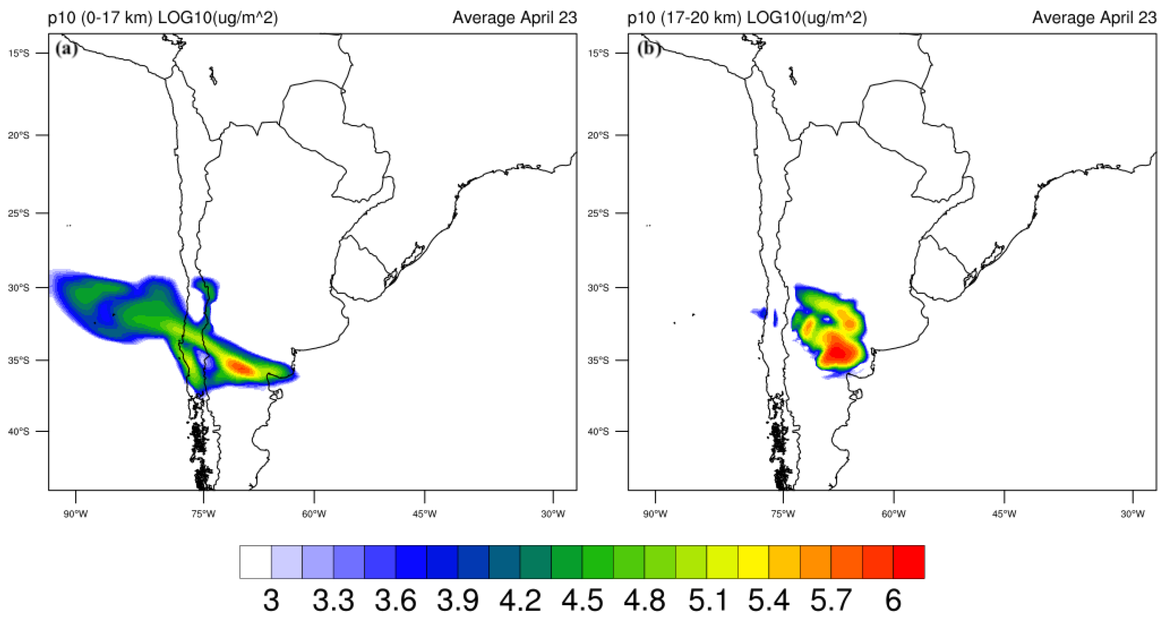
In the following Figure A1 - Figure A5 is reported the vertical integration of p10 variable (from GCTS1 simulation) that when scaled with the air density it gives g units. It is calculated as the sum of finest ash bins in the following way:
In each figure panel-a refers to the integration between 0-17 km and panel-b between 17-20 km.
Figure A1.
April 23, daily averaged vertical integrated concentration (p10) between 0-17 km (a) and 17-20 km (b); Units are g .
Figure A1.
April 23, daily averaged vertical integrated concentration (p10) between 0-17 km (a) and 17-20 km (b); Units are g .
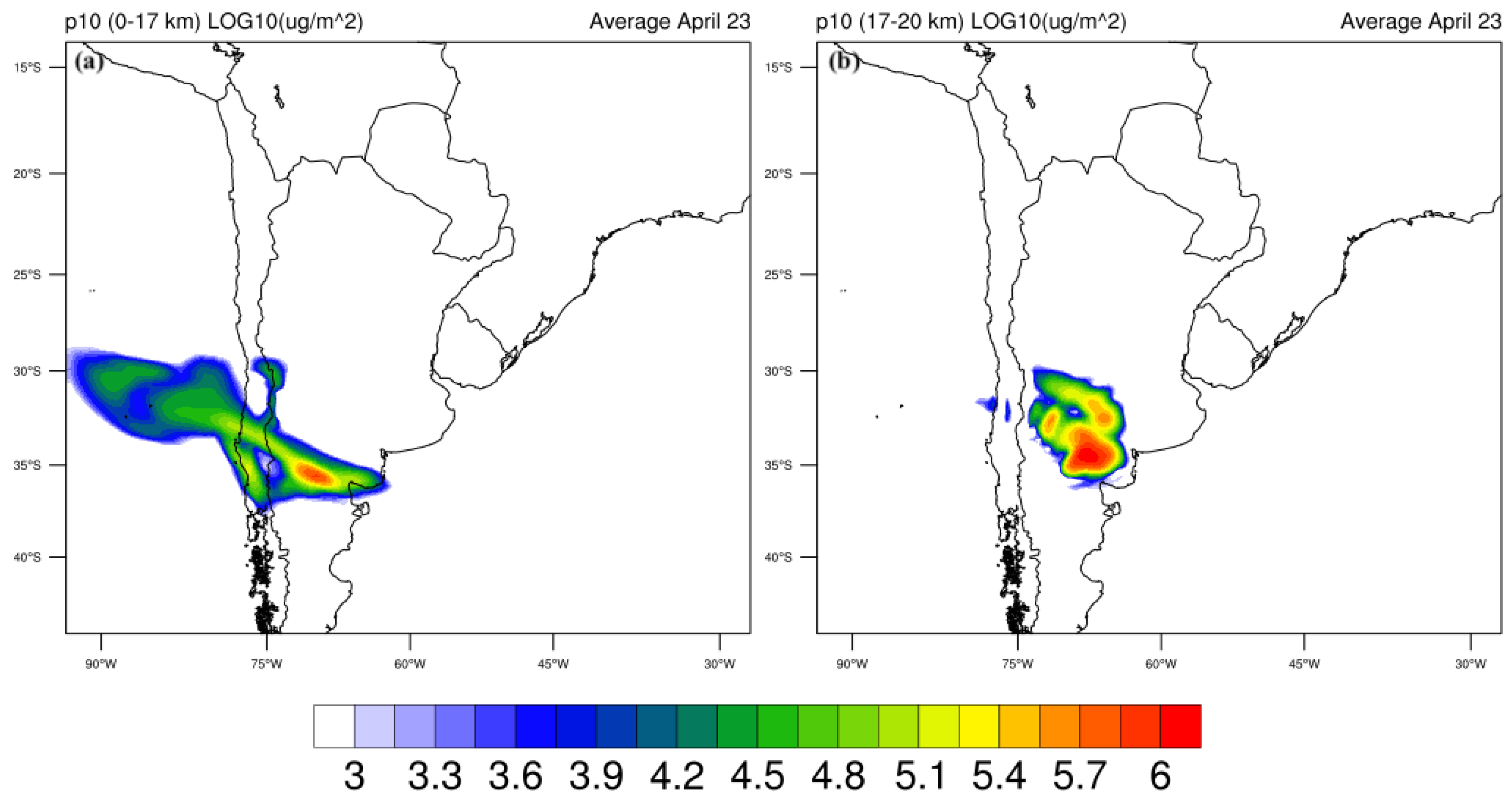
Figure A2.
April 24, daily averaged vertical integrated concentration (p10) between 0-17 km (a) and 17-20 km (b); Units are g .
Figure A2.
April 24, daily averaged vertical integrated concentration (p10) between 0-17 km (a) and 17-20 km (b); Units are g .
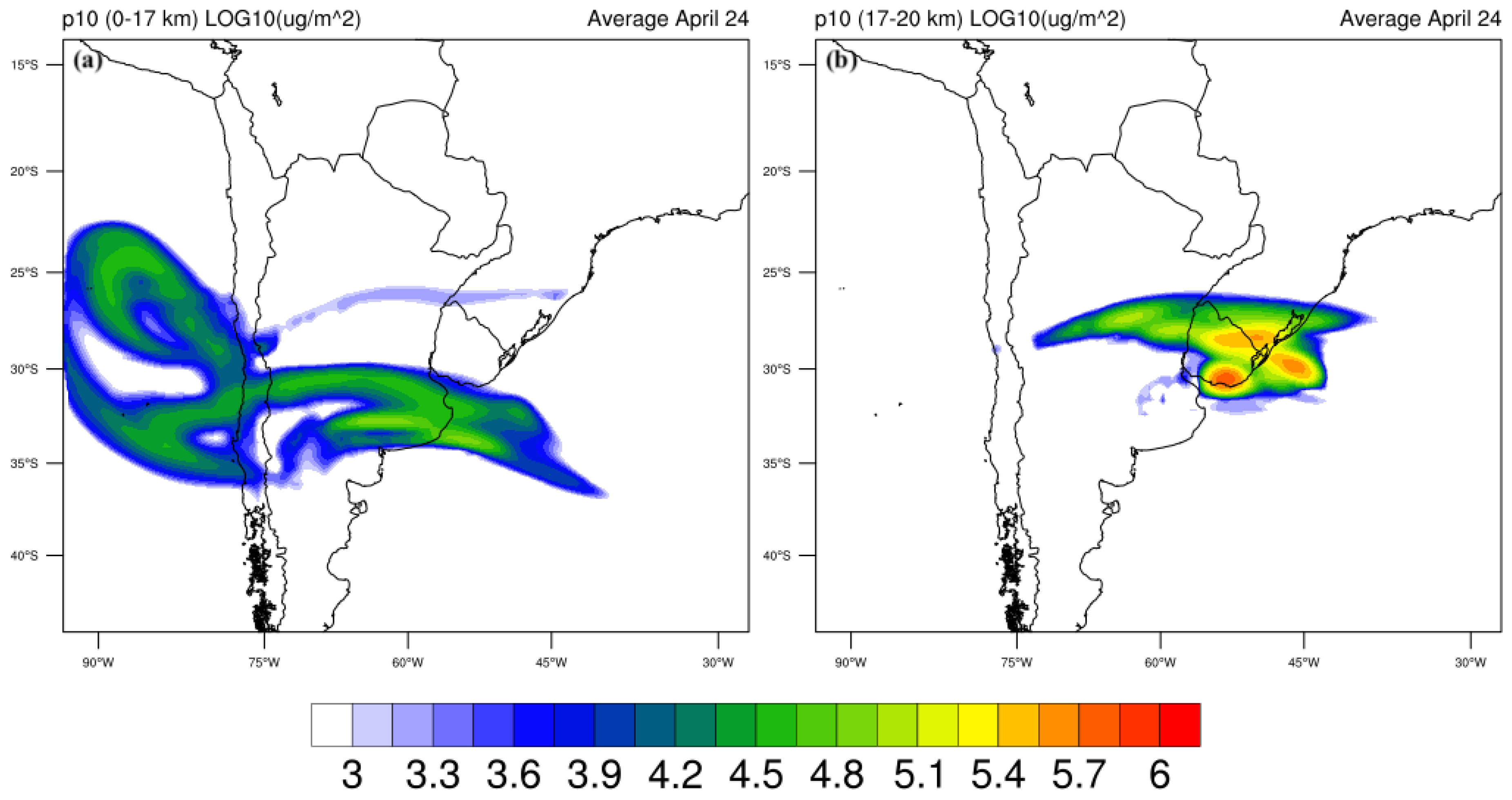
Figure A3.
April 25, daily averaged vertical integrated concentration (p10) between 0-17 km (a) and 17-20 km (b); Units are g .
Figure A3.
April 25, daily averaged vertical integrated concentration (p10) between 0-17 km (a) and 17-20 km (b); Units are g .
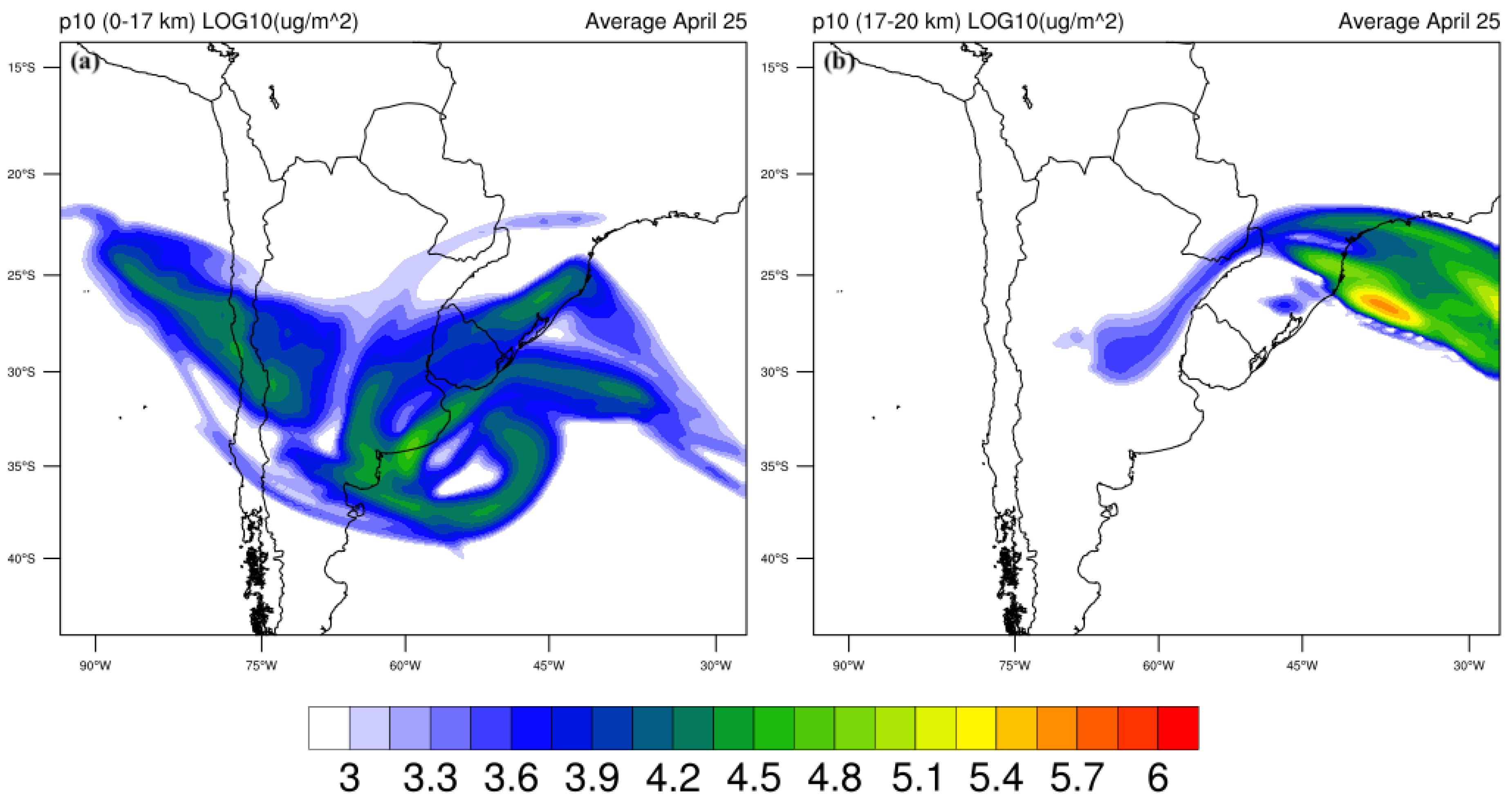
Figure A4.
April 26, daily averaged vertical integrated concentration (p10) between 0-17 km (a) and 17-20 km (b); Units are g .
Figure A4.
April 26, daily averaged vertical integrated concentration (p10) between 0-17 km (a) and 17-20 km (b); Units are g .

Figure A5.
April 27, daily averaged vertical integrated concentration (p10) between 0-17 km (a) and 17-20 km (b); Units are g .
Figure A5.
April 27, daily averaged vertical integrated concentration (p10) between 0-17 km (a) and 17-20 km (b); Units are g .
References
- Ramaswamy, V.; Collins, W.; Haywood, J.; Lean, J.; Mahowald, N.; Myhre, G.; Naik, V.; Shine, K.P.; Soden, B.; Stenchikov, G.; others. Radiative forcing of climate: The historical evolution of the radiative forcing concept, the forcing agents and their quantification, and applications. Meteorological Monographs 2019, 59, 14–1. [Google Scholar] [CrossRef]
- Charlson, R.J.; Schwartz, S.; Hales, J.; Cess, R.D.; Coakley Jr, J.; Hansen, J.; Hofmann, D. Climate forcing by anthropogenic aerosols. Science 1992, 255, 423–430. [Google Scholar] [CrossRef] [PubMed]
- Twomey, S. The influence of pollution on the shortwave albedo of clouds. Journal of the atmospheric sciences 1977, 34, 1149–1152. [Google Scholar] [CrossRef]
- Textor, C.; Graf, H.F.; Timmreck, C.; Robock, A. Emissions from volcanoes. In Emissions of atmospheric trace compounds; Springer, 2004; pp. 269–303. [CrossRef]
- Arghavani, S.; Rose, C.; Banson, S.; Lupascu, A.; Gouhier, M.; Sellegri, K.; Planche, C. The effect of using a new parameterization of nucleation in the WRF-Chem model on new particle formation in a passive volcanic plume. Atmosphere 2021, 13, 15. [Google Scholar] [CrossRef]
- Tsigaridis, K.; Krol, M.; Dentener, F.; Balkanski, Y.; Lathiere, J.; Metzger, S.; Hauglustaine, D.; Kanakidou, M. Change in global aerosol composition since preindustrial times. Atmospheric Chemistry and Physics 2006, 6, 5143–5162. [Google Scholar] [CrossRef]
- McCormick, M.P.; Thomason, L.W.; Trepte, C.R. Atmospheric effects of the Mt Pinatubo eruption. Nature 1995, 373, 399–404. [Google Scholar] [CrossRef]
- Sellitto, P.; Podglajen, A.; Belhadji, R.; Boichu, M.; Carboni, E.; Cuesta, J.; Duchamp, C.; Kloss, C.; Siddans, R.; Bègue, N.; others. The unexpected radiative impact of the Hunga Tonga eruption of 15th January 2022. Communications Earth & Environment 2022, 3, 288. [Google Scholar] [CrossRef]
- Stern, C.R.; Moreno, H.; López-Escobar, L.; Clavero, J.E.; Lara, L.E.; Naranjo, J.A.; Parada, M.A.; Skewes, M.A. Chilean volcanoes 2007.
- Newhall, C.G.; Self, S. The volcanic explosivity index (VEI) an estimate of explosive magnitude for historical volcanism. Journal of Geophysical Research: Oceans 1982, 87, 1231–1238. [Google Scholar] [CrossRef]
- González-Ferrán, O. Volcanes de Chile. Instituto Geográfico Militar. Santiago 1995, 635. [Google Scholar]
- Petit-Breuilh, M. Cronologia eruptiva historica de los volcanes Osorno y Calbuco, Andes del Sur (41∘-41∘30’s); Servicio Nacional de Geología y Minería, 1999.
- Daga, R.; Guevara, S.R.; Poire, D.G.; Arribére, M. Characterization of tephras dispersed by the recent eruptions of volcanoes Calbuco (1961), Chaitén (2008) and Cordón Caulle Complex (1960 and 2011), in Northern Patagonia. Journal of South American Earth Sciences 2014, 49, 1–14. [Google Scholar] [CrossRef]
- Bègue, N.; Vignelles, D.; Berthet, G.; Portafaix, T.; Payen, G.; Jégou, F.; Bencherif, H.; Jumelet, J.; Vernier, J.P.; Lurton, T.; others. Long-range transport of stratospheric aerosols in the Southern Hemisphere following the 2015 Calbuco eruption. Atmospheric Chemistry and Physics 2017, 17, 15019–15036. [Google Scholar] [CrossRef]
- JS Lopes, F.; Silva, J.J.; Antuna Marrero, J.C.; Taha, G.; Landulfo, E. Synergetic aerosol layer observation after the 2015 calbuco volcanic eruption event. Remote Sensing 2019, 11, 195. [Google Scholar] [CrossRef]
- Van Eaton, A.R.; Amigo, Á.; Bertin, D.; Mastin, L.G.; Giacosa, R.E.; González, J.; Valderrama, O.; Fontijn, K.; Behnke, S.A. Volcanic lightning and plume behavior reveal evolving hazards during the April 2015 eruption of Calbuco volcano, Chile. Geophysical Research Letters 2016, 43, 3563–3571. [Google Scholar] [CrossRef]
- Romero, J.; Morgavi, D.; Arzilli, F.; Daga, R.; Caselli, A.; Reckziegel, F.; Viramonte, J.; Díaz-Alvarado, J.; Polacci, M.; Burton, M.; others. Eruption dynamics of the 22–23 April 2015 Calbuco Volcano (Southern Chile): Analyses of tephra fall deposits. Journal of Volcanology and Geothermal Research 2016, 317, 15–29. [Google Scholar] [CrossRef]
- Marzano, F.S.; Corradini, S.; Mereu, L.; Kylling, A.; Montopoli, M.; Cimini, D.; Merucci, L.; Stelitano, D. Multisatellite multisensor observations of a Sub-Plinian volcanic eruption: the 2015 Calbuco explosive event in Chile. IEEE Transactions on Geoscience and Remote Sensing 2018, 56, 2597–2612. [Google Scholar] [CrossRef]
- Mastin, L.G.; Van Eaton, A.R. Comparing simulations of umbrella-cloud growth and ash transport with observations from Pinatubo, Kelud, and Calbuco volcanoes. Atmosphere 2020, 11, 1038. [Google Scholar] [CrossRef]
- Schwaiger, H.F.; Denlinger, R.P.; Mastin, L.G. Ash3d: A finite-volume, conservative numerical model for ash transport and tephra deposition. Journal of Geophysical Research: Solid Earth 2012, 117. [Google Scholar] [CrossRef]
- Castorina, G.; Semprebello, A.; Gattuso, A.; Salerno, G.; Sellitto, P.; Italiano, F.; Rizza, U. Modelling Paroxysmal and Mild-Strombolian Eruptive Plumes at Stromboli and Mt. Etna on 28 August 2019. Remote Sensing 2023, 15, 5727. [Google Scholar] [CrossRef]
- Stuefer, M.; Freitas, S.; Grell, G.; Webley, P.; Peckham, S.; McKeen, S.; Egan, S. Inclusion of ash and SO 2 emissions from volcanic eruptions in WRF-Chem: Development and some applications. Geoscientific Model Development 2013, 6, 457–468. [Google Scholar] [CrossRef]
- Stenchikov, G.; Ukhov, A.; Osipov, S. Modeling of Instantaneous and Adjusted Radiative Forcing of the 2022 Hunga Volcano Explosion. Technical report, Copernicus Meetings, 2024. [CrossRef]
- Fast, J.D.; Gustafson Jr, W.I.; Easter, R.C.; Zaveri, R.A.; Barnard, J.C.; Chapman, E.G.; Grell, G.A.; Peckham, S.E. Evolution of ozone, particulates, and aerosol direct radiative forcing in the vicinity of Houston using a fully coupled meteorology-chemistry-aerosol model. Journal of Geophysical Research: Atmospheres 2006, 111. [Google Scholar] [CrossRef]
- Stenchikov, G.; Lahoti, N.; Diner, D.J.; Kahn, R.; Lioy, P.J.; Georgopoulos, P.G. Multiscale plume transport from the collapse of the World Trade Center on September 11, 2001. Environmental Fluid Mechanics 2006, 6, 425–450. [Google Scholar] [CrossRef]
- Seluchi, M.E.; Marengo, J.A. Tropical–midlatitude exchange of air masses during summer and winter in South America: Climatic aspects and examples of intense events. International Journal of Climatology: A Journal of the Royal Meteorological Society 2000, 20, 1167–1190. [Google Scholar] [CrossRef]
- Marengo, J.A.; Seluchi, M.E. Tropical mid-latitude exchange of air masses in South America. Part I: Some climatic aspects. Trabajo presentado en el VIII Congreso Latinoamericano e Ibérico de Meteorología y X Congresso Brasileiro de Meteorologia, Brasilia, Brasil, 1998.
- Gan, M.A.; Rao, V.B. The influence of the Andes Cordillera on transient disturbances. Monthly Weather Review 1994, 122, 1141–1157. [Google Scholar] [CrossRef]
- Seluchi, M.E.; Garreaud, R.; Norte, F.A.; Saulo, A.C. Influence of the subtropical Andes on baroclinic disturbances: A cold front case study. Monthly Weather Review 2006, 134, 3317–3335. [Google Scholar] [CrossRef]
- Satyamurty, P.; Dos Santos, R.P.; Lems, M.A.M. On the stationary trough generated by the Andes. Monthly Weather Review 1980, 108, 510–520. [Google Scholar] [CrossRef]
- Ivy, D.J.; Solomon, S.; Kinnison, D.; Mills, M.J.; Schmidt, A.; Neely III, R.R. The influence of the Calbuco eruption on the 2015 Antarctic ozone hole in a fully coupled chemistry-climate model. Geophysical Research Letters 2017, 44, 2556–2561. [Google Scholar] [CrossRef]
- Phillips, N.A. The general circulation of the atmosphere: A numerical experiment. Quarterly Journal of the Royal Meteorological Society 1956, 82, 123–164. [Google Scholar] [CrossRef]
- Pinheiro, H.R.; Hodges, K.I.; Gan, M.A.; Ferreira, N.J. A new perspective of the climatological features of upper-level cut-off lows in the Southern Hemisphere. Climate Dynamics 2017, 48, 541–559. [Google Scholar] [CrossRef]
- Hakim, G.J.; Uccellini, L.W. Diagnosing coupled jet-streak circulations for a northern plains snow band from the operational nested-grid model. Weather and forecasting 1992, 7, 26–48. [Google Scholar] [CrossRef]
- Uccellini, L.W.; Kocin, P.J. The interaction of jet streak circulations during heavy snow events along the east coast of the United States. Weather and Forecasting 1987, 2, 289–308. [Google Scholar] [CrossRef]
- Arzilli, F.; Morgavi, D.; Petrelli, M.; Polacci, M.; Burton, M.; Di Genova, D.; Spina, L.; La Spina, G.; Hartley, M.E.; Romero, J.E.; others. The unexpected explosive sub-Plinian eruption of Calbuco volcano (22–23 April 2015; southern Chile): Triggering mechanism implications. Journal of Volcanology and Geothermal Research 2019, 378, 35–50. [Google Scholar] [CrossRef]
- Seluchi, M.E.; Norte, F.A.; Satyamurty, P.; Chou, S.C. Analysis of three situations of the foehn effect over the Andes (zonda wind) using the Eta–CPTEC regional model. Weather and forecasting 2003, 18, 481–501. [Google Scholar] [CrossRef]
- Grell, G.A.; Peckham, S.E.; Schmitz, R.; McKeen, S.A.; Frost, G.; Skamarock, W.C.; Eder, B. Fully coupled “online” chemistry within the WRF model. Atmospheric environment 2005, 39, 6957–6975. [Google Scholar] [CrossRef]
- Chin, M.; Rood, R.B.; Lin, S.J.; Müller, J.F.; Thompson, A.M. Atmospheric sulfur cycle simulated in the global model GOCART: Model description and global properties. Journal of Geophysical Research: Atmospheres 2000, 105, 24671–24687. [Google Scholar] [CrossRef]
- Mastin, L.G.; Guffanti, M.; Servranckx, R.; Webley, P.; Barsotti, S.; Dean, K.; Durant, A.; Ewert, J.W.; Neri, A.; Rose, W.I.; others. A multidisciplinary effort to assign realistic source parameters to models of volcanic ash-cloud transport and dispersion during eruptions. Journal of volcanology and Geothermal Research 2009, 186, 10–21. [Google Scholar] [CrossRef]
- Steensen, T.; Stuefer, M.; Webley, P.; Grell, G.; Freitas, S. Qualitative comparison of Mount Redoubt 2009 volcanic clouds using the PUFF and WRF-Chem dispersion models and satellite remote sensing data. Journal of Volcanology and Geothermal Research 2013, 259, 235–247. [Google Scholar] [CrossRef]
- Scollo, S.; Del Carlo, P.; Coltelli, M. Tephra fallout of 2001 Etna flank eruption: Analysis of the deposit and plume dispersion. Journal of Volcanology and Geothermal Research 2007, 160, 147–164. [Google Scholar] [CrossRef]
- Rose, W.I.; Durant, A.J. Fine ash content of explosive eruptions. Journal of Volcanology and Geothermal Research 2009, 186, 32–39. [Google Scholar] [CrossRef]
- Freitas, S.R.; Longo, K.M.; Alonso, M.a.; Pirre, M.; Marécal, V.; Grell, G.; Stockler, R.; Mello, R.; Sánchez Gácita, M. PREP-CHEM-SRC–1.0: a preprocessor of trace gas and aerosol emission fields for regional and global atmospheric chemistry models. Geoscientific Model Development 2011, 4, 419–433. [Google Scholar] [CrossRef]
- for Environmental Prediction/National Weather Service/NOAA/US Department of Commerce, N.C. NCEP GDAS/FNL 0.25 degree global tropospheric analyses and forecast grids, research data archive at the National Center for Atmospheric Research, Computational and Information Systems Laboratory 2015. [CrossRef]
- Sparks, R.S.J.; Bursik, M.; Carey, S.; Gilbert, J.; Glaze, L.; Sigurdsson, H.; Woods, A. Volcanic plumes; John Wiley & Sons, Inc, 1997.
- Olson, J.B.; Kenyon, J.S.; Angevine, W.; Brown, J.M.; Pagowski, M.; Sušelj, K.; others. A description of the MYNN-EDMF scheme and the coupling to other components in WRF–ARW 2019. [CrossRef]
- Olson, J.B.; Smirnova, T.; Kenyon, J.S.; Turner, D.D.; Brown, J.M.; Zheng, W.; Green, B.W. A description of the MYNN surface-layer scheme 2021. [CrossRef]
- Smirnova, T.G.; Brown, J.M.; Benjamin, S.G.; Kenyon, J.S. Modifications to the rapid update cycle land surface model (RUC LSM) available in the weather research and forecasting (WRF) model. Monthly weather review 2016, 144, 1851–1865. [Google Scholar] [CrossRef]
- Nakanishi, M.; Niino, H. An improved Mellor–Yamada level-3 model with condensation physics: Its design and verification. Boundary-layer meteorology 2004, 112, 1–31. [Google Scholar] [CrossRef]
- Morrison, H.; Thompson, G.; Tatarskii, V. Impact of cloud microphysics on the development of trailing stratiform precipitation in a simulated squall line: Comparison of one-and two-moment schemes. Monthly weather review 2009, 137, 991–1007. [Google Scholar] [CrossRef]
- Morrison, H.; Milbrandt, J.A.; Bryan, G.H.; Ikeda, K.; Tessendorf, S.A.; Thompson, G. Parameterization of cloud microphysics based on the prediction of bulk ice particle properties. Part II: Case study comparisons with observations and other schemes. Journal of the Atmospheric Sciences 2015, 72, 312–339. [Google Scholar] [CrossRef]
- Hsu, N.; Jeong, M.J.; Bettenhausen, C.; Sayer, A.; Hansell, R.; Seftor, C.; Huang, J.; Tsay, S.C. Enhanced Deep Blue aerosol retrieval algorithm: The second generation. Journal of Geophysical Research: Atmospheres 2013, 118, 9296–9315. [Google Scholar] [CrossRef]
- Kaufman, Y.; Tanré, D.; Remer, L.A.; Vermote, E.; Chu, A.; Holben, B. Operational remote sensing of tropospheric aerosol over land from EOS moderate resolution imaging spectroradiometer. Journal of Geophysical Research: Atmospheres 1997, 102, 17051–17067. [Google Scholar] [CrossRef]
- Sayer, A.M.; Hsu, N.C.; Bettenhausen, C.; Holz, R.E.; Lee, J.; Quinn, G.; Veglio, P. Cross-calibration of S-NPP VIIRS moderate-resolution reflective solar bands against MODIS Aqua over dark water scenes. Atmospheric Measurement Techniques 2017, 10, 1425–1444. [Google Scholar] [CrossRef]
- Prata, A. Infrared radiative transfer calculations for volcanic ash clouds. Geophysical research letters 1989, 16, 1293–1296. [Google Scholar] [CrossRef]
- Sayer, A.; Hsu, N.; Lee, J.; Bettenhausen, C.; Kim, W.; Smirnov, A. Satellite Ocean Aerosol Retrieval (SOAR) algorithm extension to S-NPP VIIRS as part of the “Deep Blue” aerosol project. Journal of Geophysical Research: Atmospheres 2018, 123, 380–400. [Google Scholar] [CrossRef]
| 1 | |
| 2 | |
| 3 |
Figure 1.
Synoptic fields on April 23 at 00:00 UTC from the WRF model: a) Wind field at 850 hPa; b) Wind field up to 200 hPa; c) Surface Pressure (isolines) and thickness 500-1000 hPa field (shaded contours); d) Geopotential at 500 hPa (isolines) and relative vorticity field (shaded contours). The blue dot indicates the region of the Calbuco volcano.
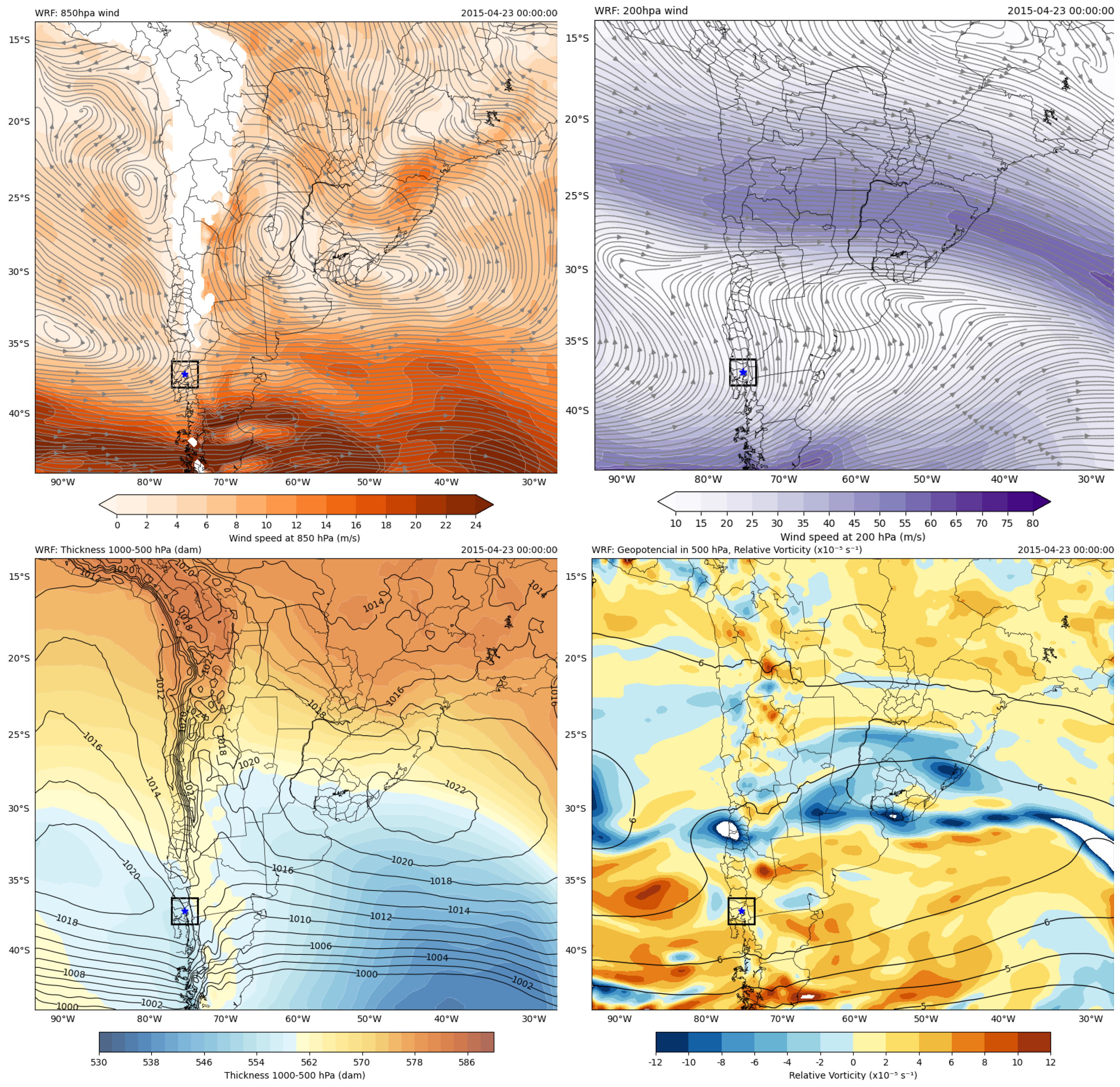
Figure 2.
Synoptic fields on April 24 at 00:00 UTC from the WRF model: a) Wind field at 850 hPa; b) Wind field up to 200 hPa; c) Surface Pressure (isolines) and thickness 500-1000 hPa field (shaded contours); d) Geopotential at 500 hPa (isolines) and relative vorticity field (shaded contours). The blue dot indicates the region of the Calbuco volcano.
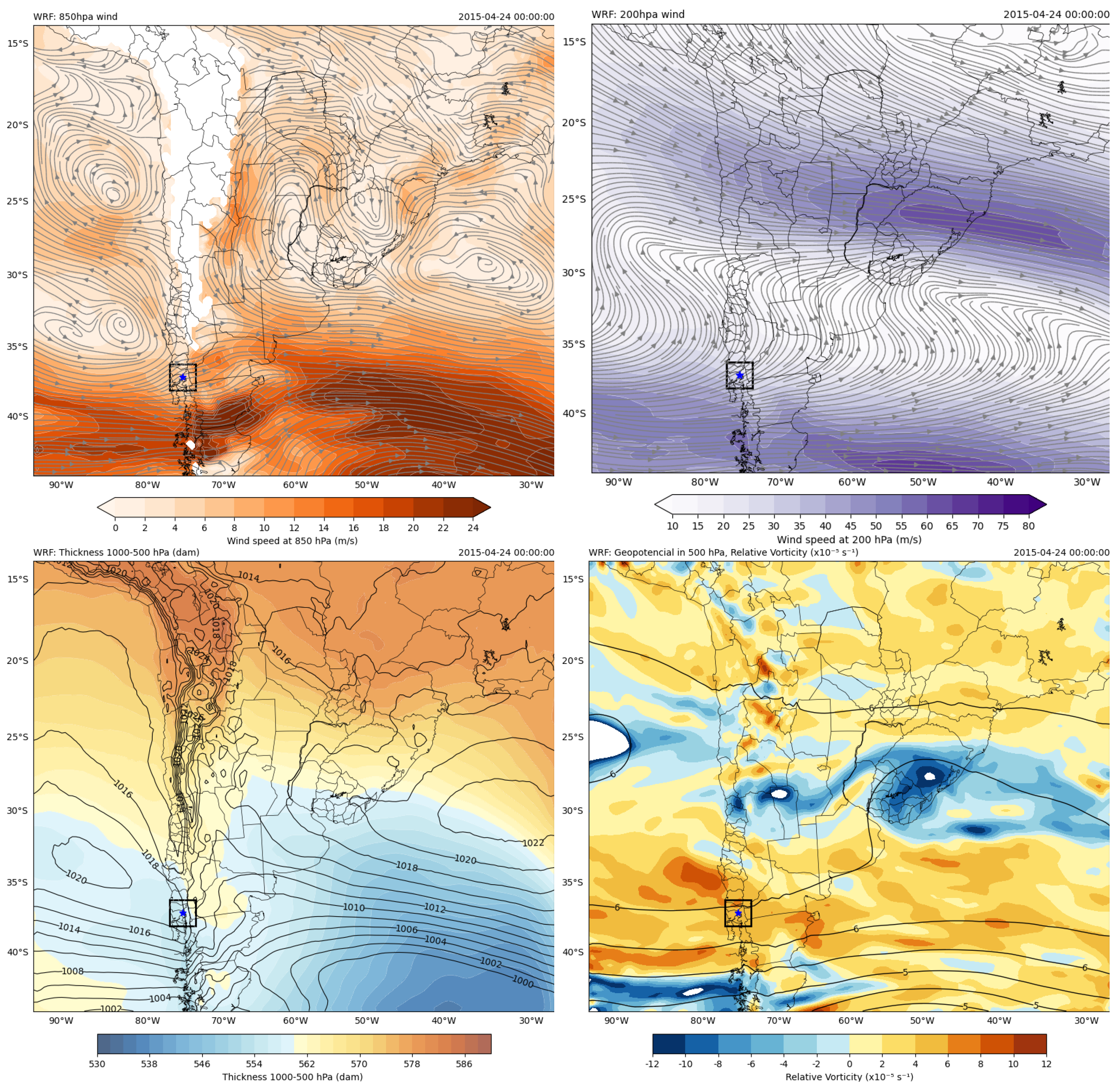
Figure 3.
Synoptic fields on April 25 at 00:00 UTC from the WRF model: a) Wind field at 850 hPa; b) Wind field up to 200 hPa; c) Surface Pressure (isolines) and thickness 500-1000 hPa field (shaded contours); d) Geopotential at 500 hPa (isolines) and relative vorticity field (shaded contours). The blue dot indicates the region of the Calbuco volcano.
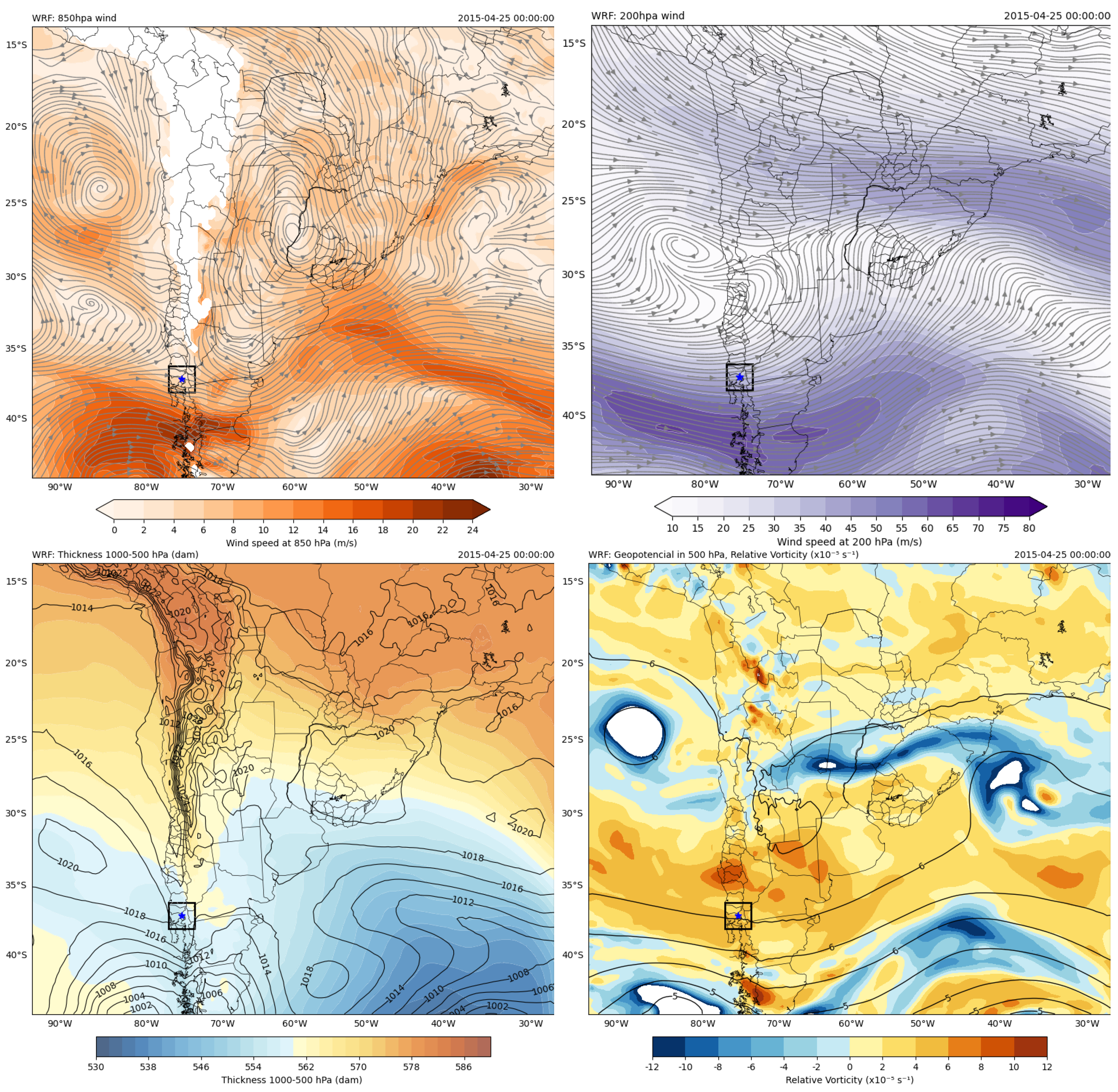
Figure 4.
Synoptic fields on April 26 at 00:00 UTC from the WRF model: a) Wind field at 850 hPa; b) Wind field up to 200 hPa; c) Surface Pressure (isolines) and thickness 500-1000 hPa field (shaded contours); d) Geopotential at 500 hPa (isolines) and relative vorticity field (shaded contours). The blue dot indicates the region of the Calbuco volcano.
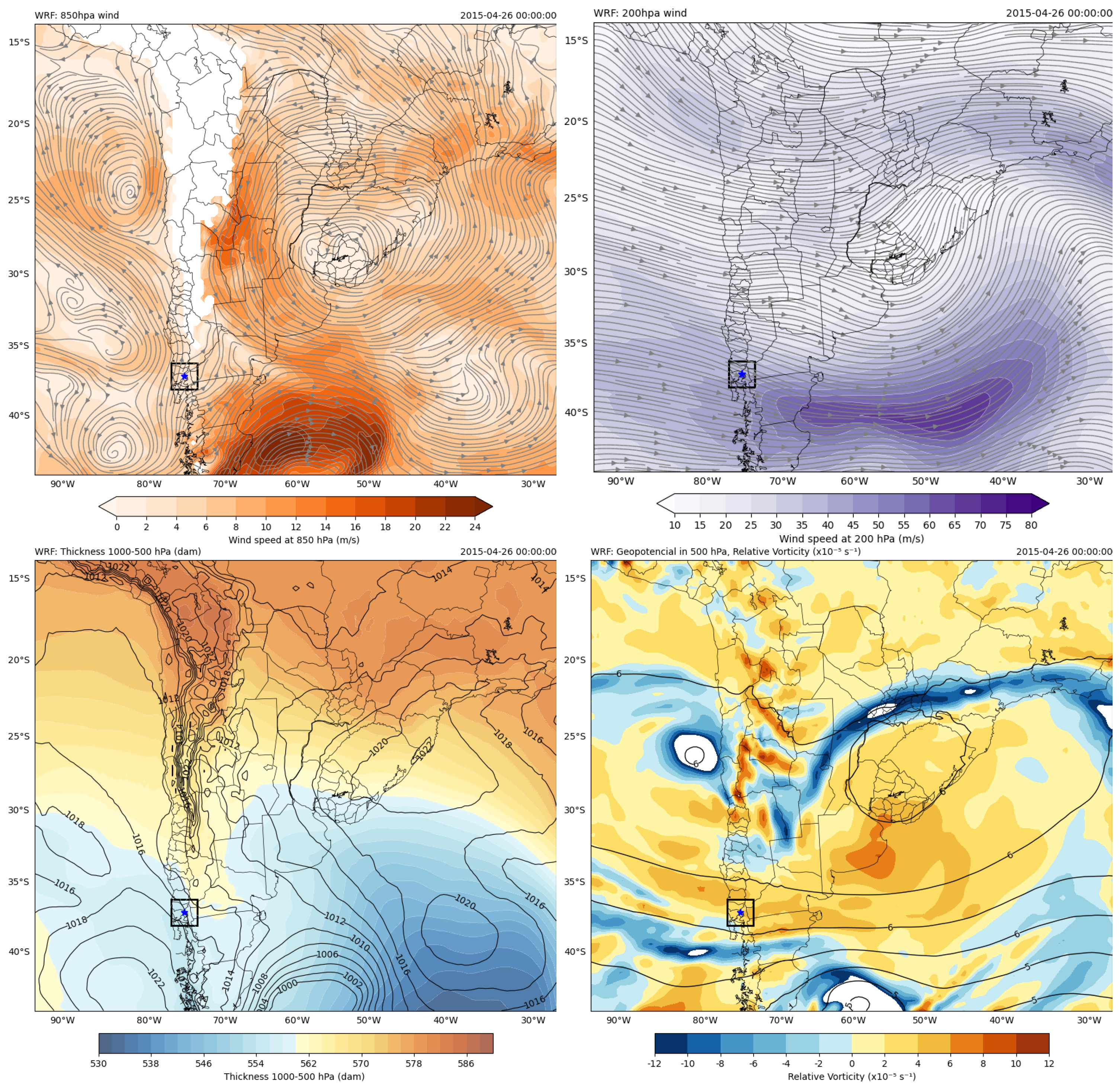
Figure 5.
Domain numerical grid and the location of Calbuco (red point).
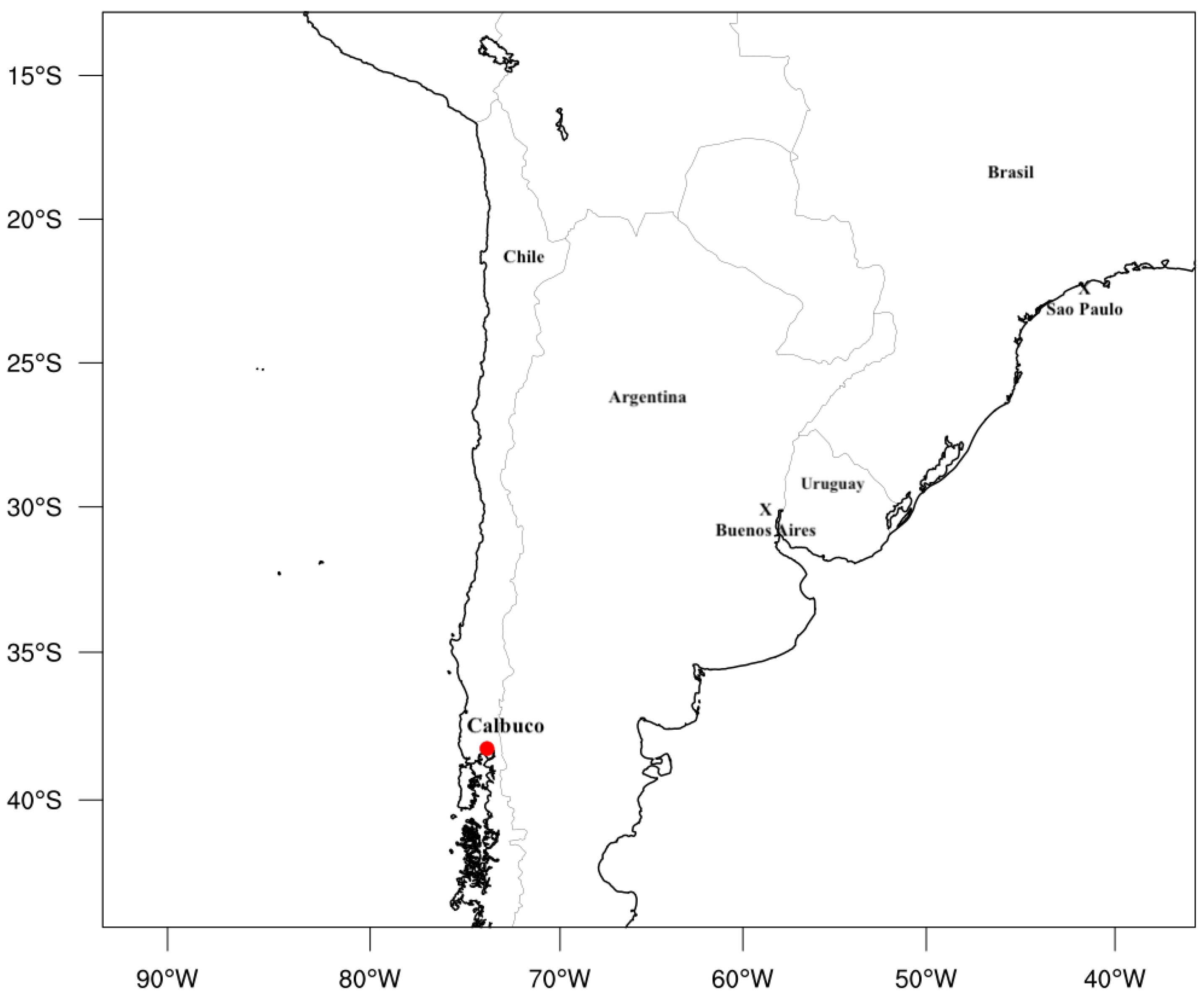
Figure 6.
Daily average AOD from AERDB (SNPP-D3-VIIRS); (a) April 23; (b) April 24; (c) April 25; (d) April 26.
Figure 6.
Daily average AOD from AERDB (SNPP-D3-VIIRS); (a) April 23; (b) April 24; (c) April 25; (d) April 26.
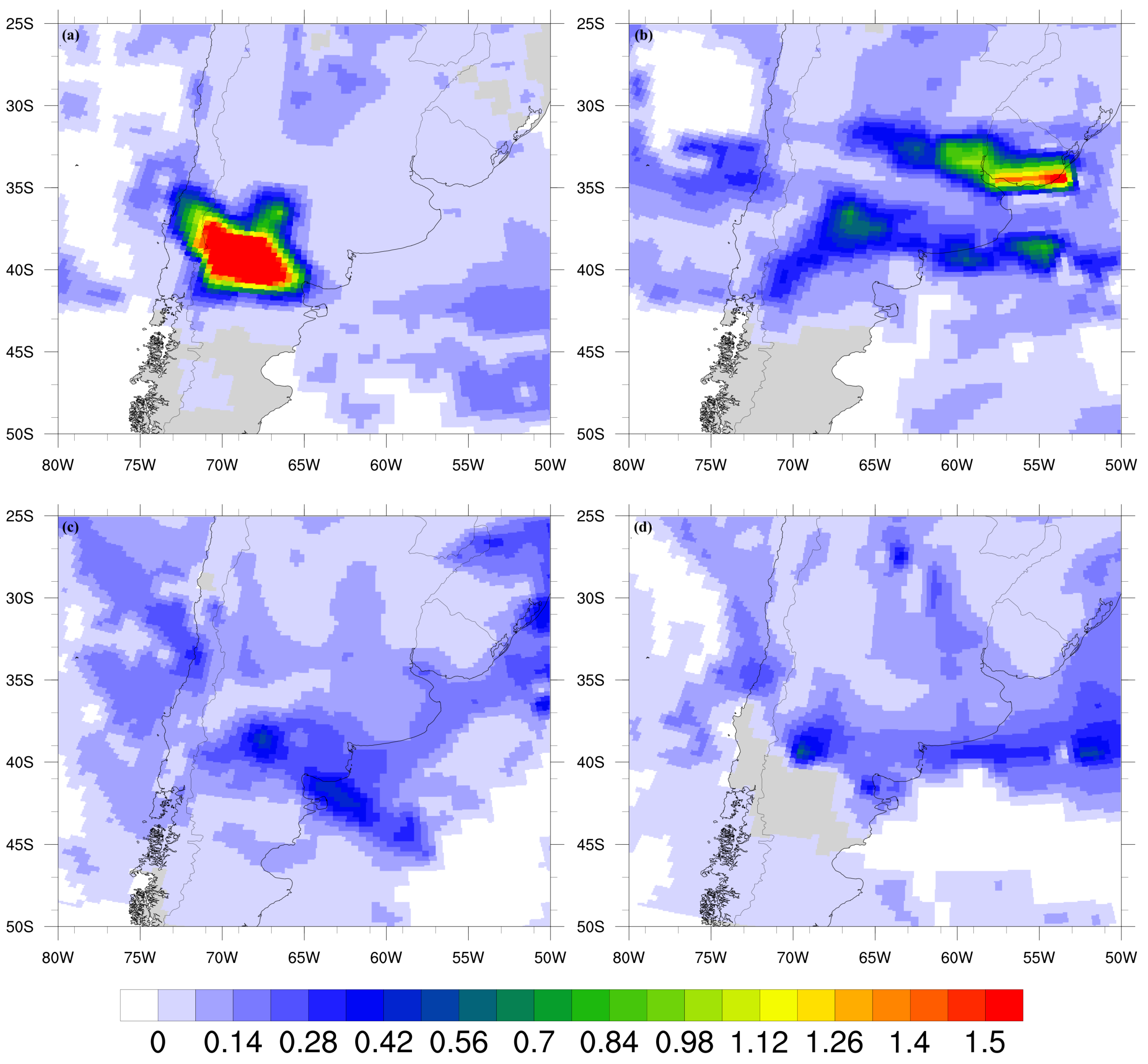
Figure 7.
Brightness Temperature Difference (BTD) along the southern region of South America for (a) April 23; (b) April 24; (c) April 25 and (d) April 26. Units are °K.
Figure 7.
Brightness Temperature Difference (BTD) along the southern region of South America for (a) April 23; (b) April 24; (c) April 25 and (d) April 26. Units are °K.
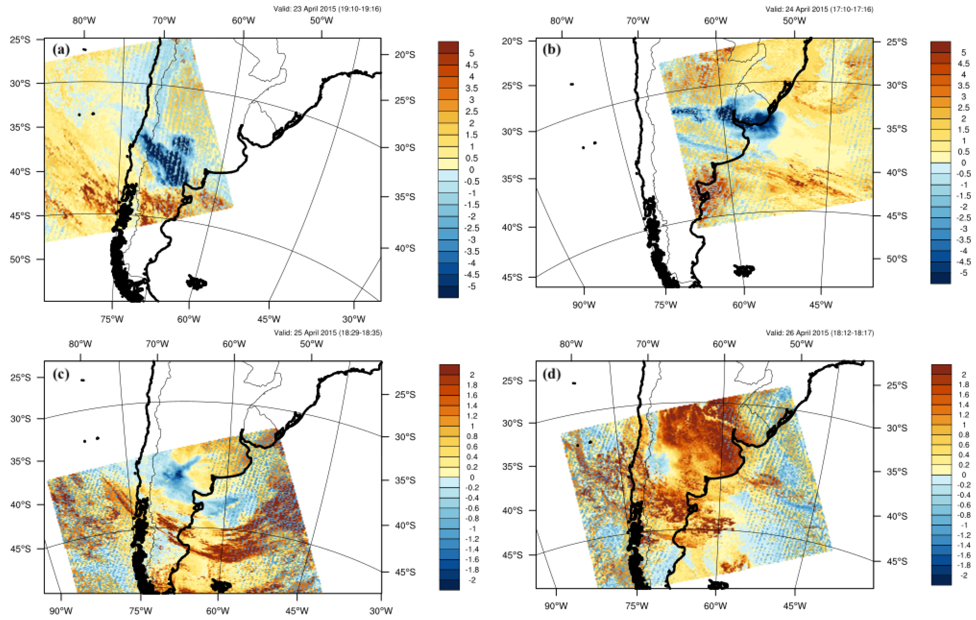
Figure 8.
Model maps of AOD at 0.55 m on April 23 for (a) AOD-GCTS2; (b) AOD-GCTS1; April 24 for (c) AOD-GCTS2; (d) AOD-GCTS1; April 25 for (e) AOD-GCTS2; (f) AOD-GCTS1.
Figure 8.
Model maps of AOD at 0.55 m on April 23 for (a) AOD-GCTS2; (b) AOD-GCTS1; April 24 for (c) AOD-GCTS2; (d) AOD-GCTS1; April 25 for (e) AOD-GCTS2; (f) AOD-GCTS1.
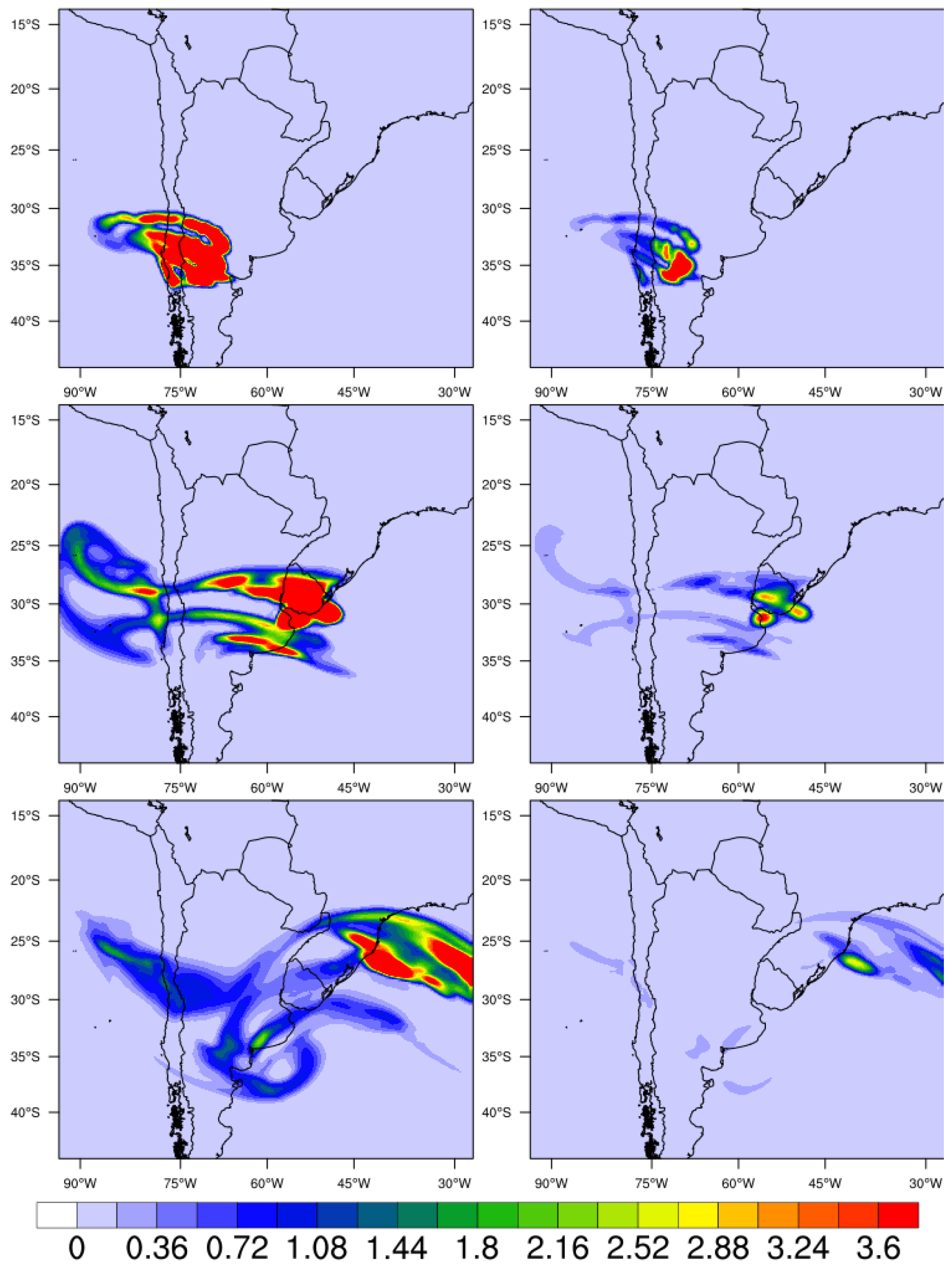
Figure 9.
(a) OMI+OMPS SO2 retrievals in Dobson Units for April 23, 2015 between 17:08 and 20:26 UTC; (b) WRF-Chem SO2 prediction for April 23, 19 UTC.
Figure 9.
(a) OMI+OMPS SO2 retrievals in Dobson Units for April 23, 2015 between 17:08 and 20:26 UTC; (b) WRF-Chem SO2 prediction for April 23, 19 UTC.
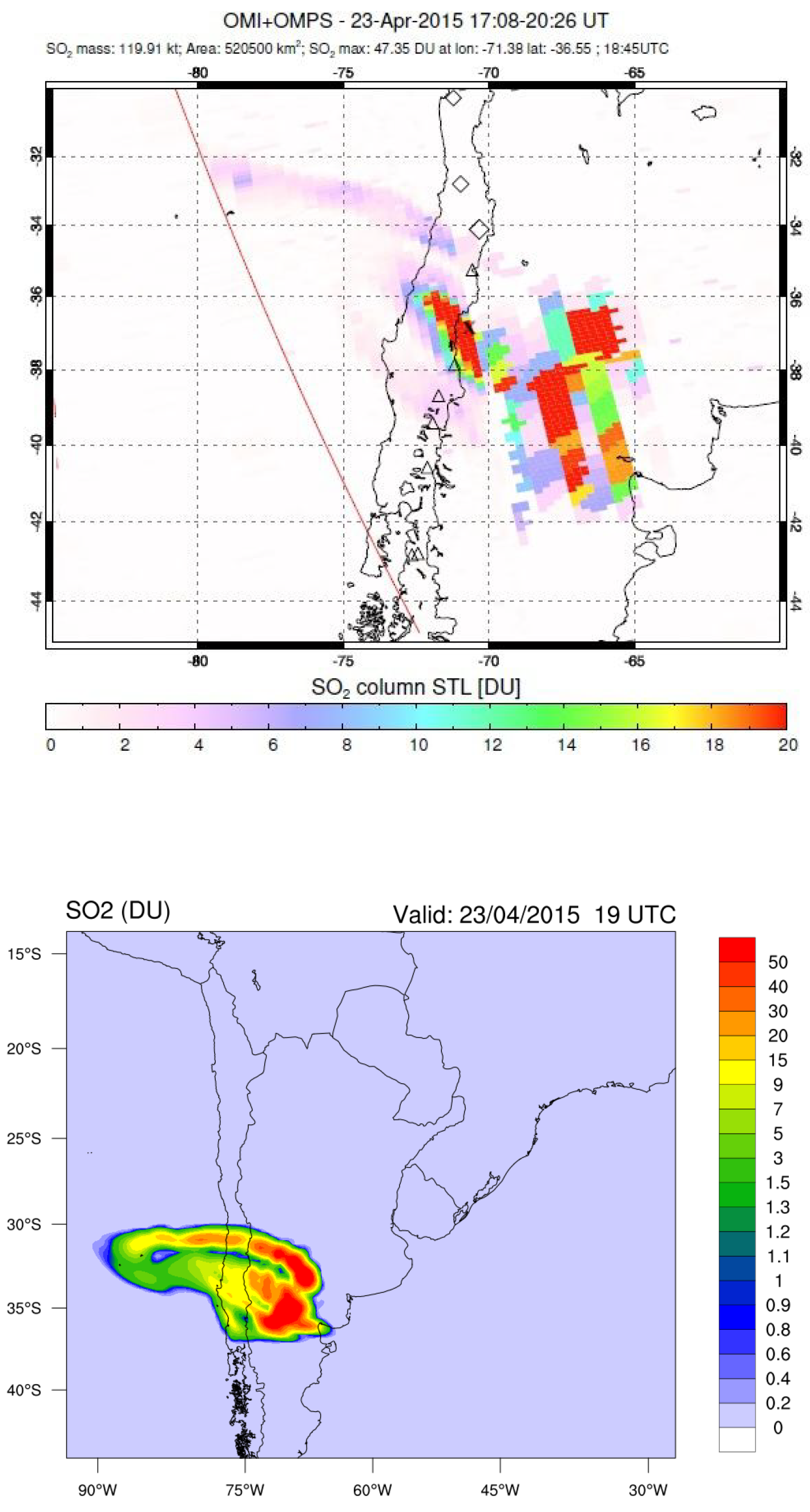
Figure 10.
(a)OMI+OMPS SO2 retrievals in Dobson Units for April 24, 2015 between 16:10 and 19:32 UTC; (b) WRF-Chem SO2 prediction for April 24, 19 UTC.
Figure 10.
(a)OMI+OMPS SO2 retrievals in Dobson Units for April 24, 2015 between 16:10 and 19:32 UTC; (b) WRF-Chem SO2 prediction for April 24, 19 UTC.
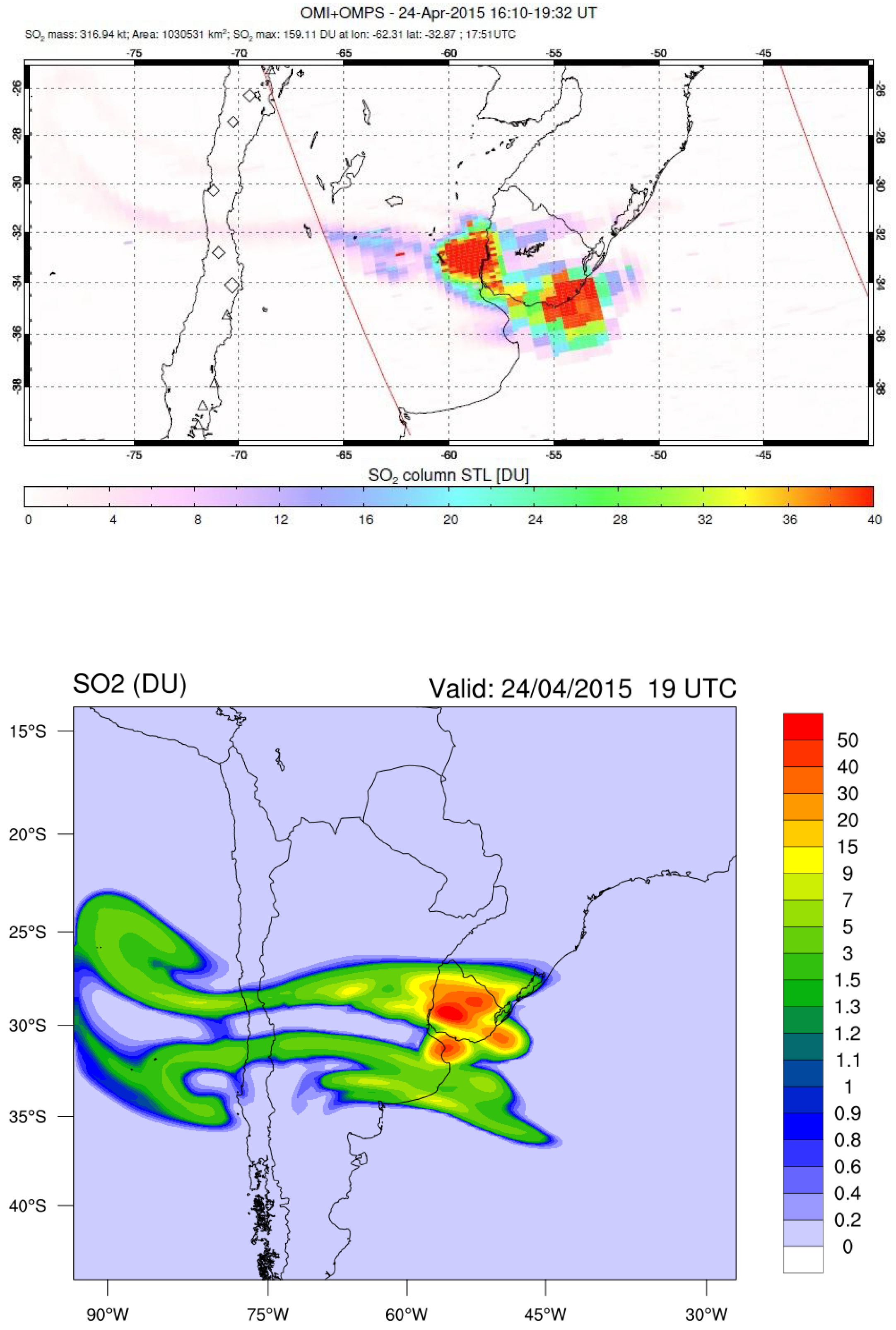
Figure 11.
a) OMI+OMPS SO2 retrievals in Dobson Units for April 25, 2015 between 15:13 and 20:11 UTC; (b) WRF-Chem SO2 prediction for April 25, 16 UTC.
Figure 11.
a) OMI+OMPS SO2 retrievals in Dobson Units for April 25, 2015 between 15:13 and 20:11 UTC; (b) WRF-Chem SO2 prediction for April 25, 16 UTC.
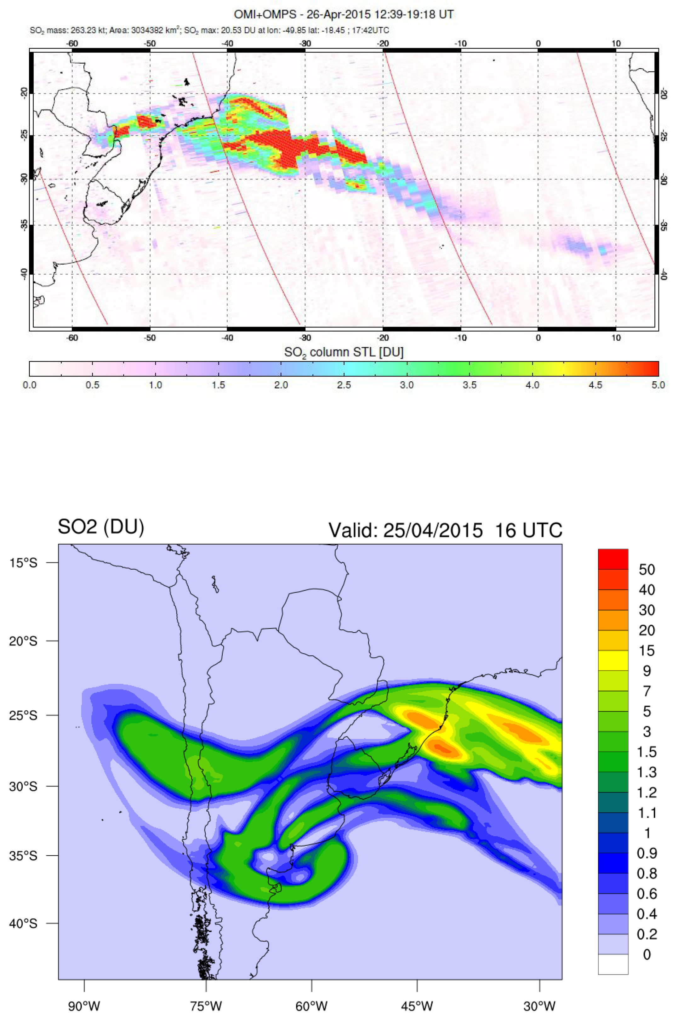
Figure 12.
(a) OMI+OMPS SO2 retrievals in Dobson Units for April 26, 2015 between 12:39 and 19:18 UTC; (b) WRF-Chem SO2 prediction for April 26, 16 UTC.
Figure 12.
(a) OMI+OMPS SO2 retrievals in Dobson Units for April 26, 2015 between 12:39 and 19:18 UTC; (b) WRF-Chem SO2 prediction for April 26, 16 UTC.
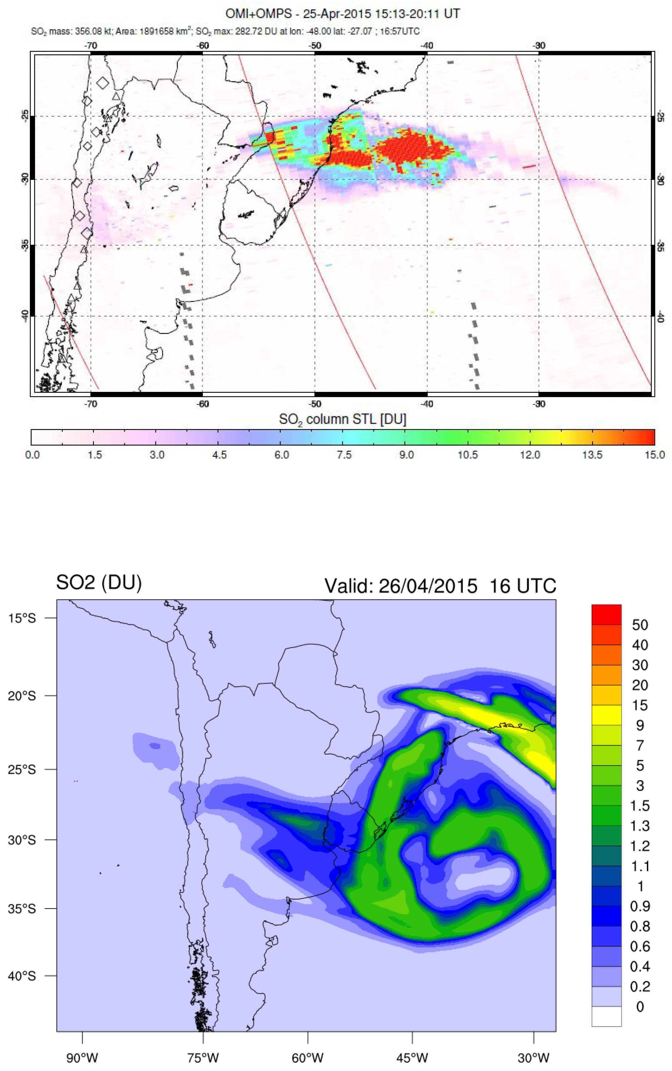
Table 2.
Ash particle bin size ranges with corresponding WRF-Chem variable name, the mass fractions in percent of the total mass is given for each ESP type-S.
Table 2.
Ash particle bin size ranges with corresponding WRF-Chem variable name, the mass fractions in percent of the total mass is given for each ESP type-S.
| var | Size bins | S0 | S1 | S2 | S3 | S8 | S9 |
| vash_1 | 1-2 mm | 22.0 | 24.0 | 22.0 | 2.9 | 2.9 | 0.0 |
| vash_2 | 0.5-1 mm | 5.0 | 25.0 | 5.0 | 3.6 | 3.6 | 0.0 |
| vash_3 | 0.25-0.5 mm | 4.0 | 20.0 | 4.0 | 11.8 | 11.8 | 0.0 |
| vash_4 | 125-250 µm | 5.0 | 12.0 | 5.0 | 8.2 | 8.2 | 9.0 |
| vash_5 | 62.5-125 µm | 24.5 | 9.0 | 24.5 | 7.9 | 7.9 | 22.0 |
| vash_6 | 31.25-62.5 µm | 12.0 | 4.3 | 12.0 | 13.0 | 13.0 | 23.0 |
| vash_7 | 15.625-31.25 µm | 11.0 | 3.3 | 11.0 | 16.3 | 16.3 | 21.0 |
| vash_8 | 7.8125-15.625 µm | 8.0 | 1.3 | 8.0 | 15.0 | 15.0 | 18.0 |
| vash_9 | 3.9065-7.8125 µm | 5.0 | 0.6 | 5.0 | 10.0 | 10.0 | 7.0 |
| vash_10 | <3.9065 µm | 3.0 | 0.5 | 3.5 | 11.2 | 11.2 | 0.0 |
Table 4.
Time granules over South America of the SUOMI-NPP spacecraft for April 2015, 23 to 26.
| day | granule time |
| 23 | 19:10 - 19:16 |
| 24 | 17:10 - 17:16 |
| 25 | 18:29 - 18:36 |
| 26 | 18:12 - 18:17 |
Disclaimer/Publisher’s Note: The statements, opinions and data contained in all publications are solely those of the individual author(s) and contributor(s) and not of MDPI and/or the editor(s). MDPI and/or the editor(s) disclaim responsibility for any injury to people or property resulting from any ideas, methods, instructions or products referred to in the content. |
© 2024 by the authors. Licensee MDPI, Basel, Switzerland. This article is an open access article distributed under the terms and conditions of the Creative Commons Attribution (CC BY) license (http://creativecommons.org/licenses/by/4.0/).
Copyright: This open access article is published under a Creative Commons CC BY 4.0 license, which permit the free download, distribution, and reuse, provided that the author and preprint are cited in any reuse.


