
Submitted:
31 October 2024
Posted:
01 November 2024
You are already at the latest version
Abstract
In this research work, we developed a fractional-order model for the transmission dynamics of malaria, incorporating two control strategies: health education campaigns, and use of insecticides. The theoretical analysis of the model was presented, including the computation of disease-free equilibrium and basic reproduction number. We analyzed the stability of the proposed model using well formulated Lyapunov function. Furthermore, model parameter estimation was carried out using real data on malaria cases reported in Zimbabwe. We found that the fractional-order model provided a better fit to the real data compared to the classical integer-order model. Sensitivity analysis of the basic reproduction number was performed using computed partial rank correlation coefficients to assess the effect of each parameter on malaria transmission. Additionally, we conducted numerical simulations to evaluate the impact of memory effects on the spread of malaria. The simulation results indicated that the order of derivatives significantly influences the dynamics of malaria transmission. Moreover, we simulated the model to assess the effectiveness of the proposed control strategies. Overall, the interventions were found to have the potential to significantly reduce the spread of malaria within the population.
Keywords:
Zika virus disease
; model formulation
; Sensitivity analysis
; parameter estimation
; numerical simulations
1. Introduction
Malaria is a vector-borne disease caused by Plasmodium parasites, which are transmitted to humans through the bites of infected female Anopheles mosquitoes [1]. These mosquitoes, primarily of the species Anopheles gambiae and Anopheles funestus, play a significant role in the transmission cycle of malaria [2]. Malaria was first identified as a disease transmitted by mosquitoes in the early 20th century, and it remains one of the most widespread and dangerous infectious diseases, especially in tropical and subtropical regions [3]. Similar to other vector-borne diseases, such as dengue, Zika virus, and yellow fever, malaria is transmitted to humans when an infected mosquito bites a susceptible individual during a blood meal [4]. Mosquitoes become infected when they bite an individual carrying the malaria parasite, although the mosquitoes themselves do not suffer from the disease [5]. The incubation period for malaria in humans typically ranges from 7 to 30 days after exposure, depending on the specific Plasmodium species [6]. Common symptoms of malaria include fever, chills, headache, muscle pain, fatigue, and in severe cases, anemia, organ failure, and death [7]. There is currently no universal vaccine for malaria, although some vaccines have been developed with limited success. Malaria management relies on antimalarial medications, such as artemisinin-based combination therapies, and preventive measures, including insecticide-treated bed nets, indoor residual spraying, and the use of mosquito repellents [8].
Mathematical models have proven invaluable in epidemiology, offering critical insights into the transmission dynamics of malaria and aiding public health officials in developing strategies for controlling the spread of the disease [18,23]. Through the use of mathematical models, researchers can simulate various intervention scenarios, study the potential outcomes of control measures, and better understand the disease’s behavior in different populations and environments [29,35].
Fractional calculus has been widely utilized to model real-world problems, including heat conduction, control theory, chaotic systems, and biological processes [13,22,28,13]. Fractional-order calculus is a popular area that focuses on the application of non-integer order derivatives in dynamic systems [23]. Literature suggests that modeling physical and real-world problems with non-integer order derivatives is more accurate than using integer-order derivatives [39]. The primary advantage of utilizing fractional-order derivatives in disease dynamics is their ability to effectively capture the memory effects and hereditary properties of species present in biological systems [39]. Due to its ability to capture memory effects, the presence of non-local operators, and its high accuracy, fractional-order derivative has gained and attracted many researchers in developing more dynamic and efficient mathematical models [41]. Researchers and scientists have utilized fractional operators to formulate mathematical models for various epidemics, accounting for different scenarios and constraints [17,22,23]. In contrast to integer-order derivatives, fractional-order derivatives are capable of capturing the memory effects and hereditary properties present in biological systems [26]. Additionally, it has been concluded that the membranes of cells in living organisms possess fractional-order electrical conductance, which can be categorized within groups of fractional-order derivatives [27]. Furthermore, fractional-order derivatives often provide a better fit to real epidemiological data [24]. The most widely utilized fractional derivatives are the Caputo, Riemann-Liouville, and Atangana-Baleanu derivatives [28]. In recent years, mathematical models incorporating fractional derivatives have been developed and studied [23,36,37]. for instance in [36], the Atangana-Baleanu operator was used to investigate the impact of personal protective measures on the dynamics of malaria transmission. Although the authors did not validate their model with real data, their findings indicated that as the fractional-order derivative decreases from 0 to 1, the number of infections in both humans and mosquitoes declines. A fractional-order model for co-infection of malaria and COVID-19 was proposed and studied in [37]. The authors calculated the threshold quantity and used the fixed-point theorem to analyze the model. Their findings showed that by implementing preventive measures to mitigate the risks associated with malaria and COVID-19, disease transmission within the population can be significantly reduced. Mathematical model of malaria disease incorporating fractional-order derivatives was formulated and analyzed in [23]. The authors used the Euler and Adam-Bashforth-Moulton scheme to simulate the model system using estimated parameters. Overall,their results showed that fractional-order derivatives have more influence on the dynamics of malaria disease in the population. For more details on mathematical model of vector borne disease using fractional-order derivatives we refer the readers to [13,15,17,19,21,23,24] and the references therein. In this study, we formulate a fractional-order model of malaria disease transmission and study the effects of human awareness on the use of insecticides. Although various types of fractional derivatives are available in the literature, our model utilizes the fractional-order calculus based on Caputo derivatives. The decision to use the Caputo derivative was influenced by several advantages; for a constant function, the Caputo derivative equals zero, consistent with the result for integer-order differential equations. Furthermore, the Caputo fractional derivative permits the incorporation of local initial conditions in the model’s formulation [28]. Recently studies have shown that one of the possible way of minimizing the spread of malaria in the population is based on how humans aware on the use of insecticides [21]. Additionally, health education campaigns to human that rise awareness of people on how to use insecticides that kill Aedes mosquitoes may significantly have impact to prevent the spread of malaria in the population [33]. To the best of our knowledge very few of mathematical model for malaria transmission formulated and validated with reported cases malaria. Therefore in this study, we propose a fractional-order model of malaria that incorporates two control strategies namely; health education campaigns, and use of insecticides and assess their effects in preventing the spread of malaria disease in the population.
The rest of the article is organized as follows: in Section 2, Mathematical model formulation is presented, In Section 3, basic properties of the model that is; positivity of variables and boundedness of trajectories are presented, computation of reproduction number and existence of model equilibrium are presented in section 4, results and discussion is presented in section 5, and conclusion remarks complete the paper in Section 6.
2. Model Formulation
In this paper, the fractional-order model of malaria disease dynamics based on Caputo sense have been formulated and studied. The proposed model demonstrates the interplay between mosquito and human populations. Through out the document, the subscript h and v respectively denote the mosquito and human population. The human population is sub-divided into four groups based on the infection status namely; Susceptible , exposed , infectious and recovered class. Thus, the total population of human at time t is denoted by given as:
Furthermore, the total population of mosquitoes at time t is denoted by which is sub-divided into three groups namely; the susceptible , exposed , and infectious class. Thus the total population of mosquitoes at time t is defined as:
All parameters and variables of the proposed model are are considered to be non-negative, and the parameters are described as follows: and denote the new recruitment rate of human and vector respectively, and they all considered to be susceptible whenever coming from either birth or immigrants; and denote the natural mortality rate of human and vector respectively; and denote transfer rate of human and vector respectively, from exposed to infectious class; represents the natural recover rate of exposed individuals; denotes the recover rate of infected humans; we have assumed that both recovered individuals (from exposed and infected class) recover with temporary immunity. Thus, the parameter represents the warning rate of immunity for recovered humans; represents the disease induced death rate of infected humans; denotes probability of disease transmission from infected mosquito to susceptible human due to successful contact between infected vector and susceptible humans; denotes the probability of disease transmission from infected human to susceptible mosquitoes due to successful contact between infected person and susceptible vector; denotes the mosquito biting rate on the humans; Recently studies have shown that one of the possible way of minimizing the spread of malaria disease in the population is based on how community is aware on the use of prevention measures such as use of mosquito nets and insecticides that reduce the possibility of human in contact with mosquitoes. Therefore in this study we consider two control strategies namely; the use of prevention measures such as mosquito nets denoted by , and use of insecticides represented by . Based on the above assumptions, we have assumed the following flow chart and non-linear differential equations:
From the flowchart diagram in Figure 1, the dynamics of the interaction between humans and mosquitoes is given in patch i by the following system of ordinary differential equations:
3. Basic Properties
Herein, we study the basic properties of system which are essential in the proof of the stability analysis.
3.1. Positivity Of Solutions
In this section, we investigate the asymptotic behavior of orbits starting in the non-negative cone . Obviously, system , which is a differential system admits a unique maximal solution for any associated Cauchy problem. In what follows we claim the following theorem:
Theorem 1.
Let and for , the maximal solution of the Cauchy problem associated to system . Then, for all , , .
Proof.
Let
By continuity of functions and , one can see that . Let . next, we have to show that . Suppose , then one has that
and are non negative on . At at least one of the following conditions is satisfied , and . Then, from the last equation of system one has that:
Integrating Eq. (4) from 0 to yields
Similarly, one can show that , , and . This is the contradiction then, and consequently the maximal solution for the steady states
of the Cauchy problem associated to system is positive. This completes the proof. □
3.2. Boundedness Of Trajectories
We have the following result about the boundedness of trajectories of system (3).
Lemma 1.
Each non-negative solution of system (3) is bounded on .
Proof.
First of all, we separate model system 3 into two parts: the human population and the Aedes mosquito populations. Adding the first five equations of model system (3) and using equation (1), yields:
Applying the Gronwall Lemma in (5) one get the following:
With this in mind, one has that for all if . This means that: and . Using the same concept we proof that This mean that: and . This completes the proof □
Corollary 1.
4. Basic Reproduction Number and Existence of Equilibria
In this section we use the next generation method as presented in [9] to compute the threshold quantity which determines the persistence and extinction of disease in the population. It is believed that when the basic reproduction number the disease persist in the population, and dies out when . The model system (3) always has a disease-free equilibrium given by
Following the next generation matrix approach as used in [9], the non-negative matrix that denotes the generation of new infection and the non-singular matrix that denotes the disease transfer among compartments evaluated at are defined as follows;
Using (9) and (10) the basic reproduction number of the model system (3) is given by:
The basic reproduction number is defined to be the expected number of secondary cases (mosquito or human) produced in a completely susceptible population, by one infectious individual (mosquito or human, respectively) during its lifetime as infectious. The square root here is due to the fact that, the generation of secondary cases in malaria diseases require two transmission process.
Theorem 2.
If then the DFE of system (3) is globally asymptotically stable in Ω otherwise it is unstable.
Proof.
By considering only the infected compartments from (3) one can write in the following ways:
where , with F and V defined as follows
,
We can observe that by direct calculation we can verify that is a nonnegative and irreducible matrix and It follows from the Perron-Frobenius theorem [12] that has positive left eigenvector associated with that is,
Since is a positive vector, we propose the following Lyapunov function to study the global stability of disease free equilibrium:
Differentiating along solutions of (3) leads to
It can be easily verified that the largest invariant subset of where is the singleton . Therefore, by LaSalle’s invariance principle [14], is globally asymptotically stable in when . □
4.1. Local Stability of the Disease Free Equilibrium Point
In this section we analyze the local stability of the disease free equilibrium (DFE) point using the Jacobian matrix and the Routh Hurwitz criteria.
Theorem 3.
and
where as if All the roots of the polynomial are negative or have negative real part if and if the determinants of all Hurwitz matrices are positive:
Given the polynomial , where the coefficients are the real constants, define the n Hurwitz matrices using the coefficients of the characteristic polynomial:
When Routh-Hurwitz criteria simplify to and
which gives the conditions that, for and
Theorem 4
(The DFE is locally asymptomatically stable if and unstable if ). Proof: The Jacobian matrix of the system is given by:
where by
.
At the DFE the Jacobian matrix becomes:
Where by The eigenvalues of are given by solving:
To obtain which are all negative. The other four eigenvalues are obtained by solving the polynomial:
For the eigenvalues to be negative then we use the Routh-Hurwitz criterion, then we have that: and Hence this implies that and the DFE is locally asymptotically stable.
4.2. Endemic Equilibrium Point
The endemic equilibrium point of the model system (3) is obtained by simultaneously solving the below system (20) and implicitly expressed in terms of :
From the second equation of the system (19) we have the following:
substituting (20) into equation four of the system (19) and solving for we obtain:
Substituting equation (21) in first equation of the system (19) and solving for we get the following:
Substituting (22) in (20) the simplified expression for (20) becomes:
Similarly for the vector population from six of (19) we have:
And from equation five of system (19) we get the following:
substituting (25) in (24) we obtain the simplified expression of as:
Where as from equation seven of system (19) and equation (26) we have:
Therefore, equations (21)–(27) gives the endemic equilibrium point (EEP) in terms of
5. Results and Discussion
In this section, we present and analyze the numerical solution of the model utilizing the Euler and Adam-Bashforth-Moulton scheme. The numerical results provide valuable insights into the behavior of the mathematical model system and the effects of its fractional order. Initially, we selected appropriate parameter values along with the initial conditions for the classes, as and . some parameters in this model have been fitted with real data of reported cases to align with realistic of the proposed model as shown in Table 1.
5.1. Model Parameter Estimations
In this section, we perform the model fitting using the data of malaria disease for 12 years as reported in Zimbabwe to fit the proposed model (3). Some of the parameters used in the simulations were adopted from the literature as shown in table (Table 1) and some parameters were estimated using root-mean square error (RMSE) the following formula:
Where n is the number of yearly reported malaria cases for 12 years. We assumed the initial population as follows: and In addition, from the model (3) the generated new cases is obtained using the term which count for the detected cases.
Figure 2 shows the reported malaria cases for 12 years in Zimbabwe, and the simulation results in Figure 3 show (a) Model fit at to the real data of malaria cases. From simulations one can note that model (3) had good fit to the reported real cases of malaria presented in Table 2. In figure (b) we fitted the malaria cases with the classical integer and fractional-order model simultaneously and we observe that fractional-order model fits well to the reported cases of malaria compared to classical integer model.
5.2. Sensitivity Analysis
In this section, we use the Partial Rank Correlation Coefficient (PRCC) to perform a global sensitivity analysis of model (3) to identify the most significant parameters that influence the spread of disease in the population. The PRCC results of the related to the number of new cases generated in the population reveals seven key influential parameters. These include the new recruitment of human and vectors ( and ), force of infections ( and ), vector biting rate (, and incubation periods ( and ), both of which are positively correlated with . On the other hand, parameters such as health education (), use of insecticides () and recover rate of infected individuals () have negative correlation with , means that whenever these parameters increase the magnitude of decreases and hence the disease dies in the population.
Figure 5 shows global sensitivity analysis of the model (3) on to the key parameters that affect the dynamic of disease in the population. Overall, we noted that increase the parameters that represent rate of insecticides, health education campaign, and vector mortality rate lead to decrease on the number of infected humans in the population. In contrast, we observed that increase on the parameters that represent rate of infections and vector biting rate lead increase on the number infected humans. In particular one can observe that as the rate of insecticides () and vector mortality rate () above the number of infected humans dies in the population.
Figure 7 shows a contour plot of (a) as a function of (use of insecticides) and (natural recover rate of exposed vectors), (b) as the function of (use of insecticides) and (health education campaigns). we observed that when the education campaign is not implemented in the population, the use of insecticides () must be greater than to reduce to be less than unit. On the other hand, when the education campaign is implemented in the population the rate of insecticides () must be to reduce the to less than unit. This results demonstrates that to minimize the spread of malaria in the community policy markers must put effort on health education campaigns on how people can prevent themselves in contact with mosquitoes. In addition, we perform the numerical simulation of the system (3) to show the influence of parameters on the model compartments. We used the fourth-order Runge–Kutta numerical method to generate the solution and the results are presented in figure (8).
To investigate the role of memory effects on the spread of malaria disease, we numerically performed the simulation of system (3) for and as presented in Figure 9 and Figure 10 respectively. The order of derivative was varied within the reasonable range and was set to (). As mentioned in the literature that when the fractional order the fractional-order model based on Caputo derivative becomes a classical ordinary differential model. Based on the numerical illustrations, one can note that as the order of derivatives reduced from 1 the memory effects of system increases, and the model solution increase quickly, peak earlier and converge to the unique equilibrium point. In particular, for the model solution converge to the disease free equilibrium after 20 days, and for the model solutions converge to unique endemic equilibrium. Furthermore, we observed that when the fractional order approaches to 0 the memory effects become strong and the model solutions converge to their respective equilibrium point earlier than when order of derivatives approach to 1. This results was also observed in the previous studies.
5.3. Effects of insecticides use on the disease dynamics
Figure 11 shows the effect of insecticides on the spread of malaria disease, we simulated the system (3) at different values of and the other parameter value are presented in table (1). From the numerical results we observed that the use of insecticides have the potential to reduce the disease the spread of malaria in the population. In particular, one can note that for the disease persist in the population and when the magnitude of is less than unit. Thus, the disease decrease in the population. Additionally, results in Figure 12 demonstrates the effects of insecticides on reduction of new cases of malaria reported in the population and one can observe that implementing of insecticides by in the community leads to high number of reduction on reported cases of disease in the population.
5.4. Effects of health education campaigns on the disease dynamics
In Figure 13 we simulate the system (3) to show the effect of health education campaign () on malaria disease transmission. The effectiveness of health education campaigns can be enhanced by utilizing various media platforms, such as newspapers, television, and social media, to inform the public on how to protect themselves from mosquitoes that transmit the malaria disease. Based on this assertions, we numerically simulate the system (3) at , and to demonstrate the effect of health education in minimizing the spread of disease in the population. From numerical illustrations one can note that as increases the number of infection generated decreases. Additionally, we observed that implementing health education campaign alone the magnitude of transmission potential () can not be reduced to less than unit.
6. Concluding Remarks
In this study, we developed and analyzed a novel model for malaria transmission and assessed the impact of health education campaigns and the use of insecticides on the spread of disease in the population. We computed the disease-free equilibrium and derived the reproduction number of the model using the next-generation method. A sensitivity analysis of the basic reproduction number was performed using partial rank correlation coefficients to examine the relationship between the reproduction number and model parameters. Overall, we found that parameters with negative indices cause a decrease in the reproduction number when increased, while parameters with positive indices lead to an increase in the reproduction number whenever. Furthermore, we fitted the model system (3) with real data of malaria cases reported in Zimbabwe for 12 years. We observed that the fractional order model () had a good fit compared to classical model (). To investigated the impact of memory effects, we simulated the system (3) at the order of derivatives and 1. overall, we observed that as the order of derivatives have an influence on the spread of disease in the population. In particular, one can note that as the order of derivative decrease from 1 the solution behavior of the system converge to the unique equilibrium much faster compared to when the order of derivative approaches 1. Finally, we simulated the model to assess the effect of proposed interventions (health education campaign and use of insecticides). From numerical results, We observed that implementing insecticides at in the population leads to eradication of disease in the community. On the other hand, we noted that implementing health education campaign alone the disease can no be eradicated in the population. However, the formulated model in this study can be improved in future by incorporation of delays in some of the model parameters and assess the its effect on the spread of disease in the population. Furthermore, this model can be improved by considering migration on both human and vectors.
References
- Singh, Ram and ul Rehman, Attiq, (2022). A fractional-order malaria model with temporary immunity, Mathematical Analysis of Infectious Diseases, 81-101.
- Pawar, DD and Patil, WD and Raut, DK, (2021). Analysis of malaria dynamics using its fractional order mathematical model, Journal of applied mathematics & informatics, 2(39), 197-214.
- Gizaw, Ademe Kebede and Deressa, Chernet Tuge, (2024). Analysis of Age-Structured Mathematical Model of Malaria Transmission Dynamics via Classical and ABC Fractional Operators, Mathematical Problems in Engineering, 1(3855146). [CrossRef]
- Venkatesan, Priya, (2024). The 2023 WHO World malaria report,The Lancet Microbe, 3(5), e214. [CrossRef]
- Cerilo-Filho, Marcelo and Arouca, Marcelo de L and Medeiros, Estela dos S and Jesus, Myrela and Sampaio, Marrara P and Reis, Nathália F and Silva, José RS and Baptista, Andréa RS and Storti-Melo, Luciane M and Machado, Ricardo LD and others, (2024). Worldwide distribution, symptoms and diagnosis of the coinfections between malaria and arboviral diseases: A systematic review, Memórias do Instituto Oswaldo Cruz, 119, e240015. [CrossRef]
- Klepac, Petra and Hsieh, Jennifer L and Ducker, Camilla L and Assoum, Mohamad and Booth, Mark and Byrne, Isabel and Dodson, Sarity and Martin, Diana L and Turner, C Michael R and van Daalen, Kim R, (2024). Climate change, malaria and neglected tropical diseases: A scoping review, Transactions of The Royal Society of Tropical Medicine and Hygiene, trae02.
- Sugathan, Adarsh and Rao, Shamathmika and Kumar, Nayanatara Arun and Chatterjee, Pratik, (2024). Malaria and Malignancies-A review, Global Biosecurity, 6. [CrossRef]
- Patel, Priya and Bagada, Arti and Vadia, Nasir, (2024). Epidemiology and Current Trends in Malaria, Rising Contagious Diseases: Basics, Management, and Treatments, 261-282.
- van den Driessche P. and Watmough, J, (2002). Reproduction number and subthreshold endemic equilibria for compartment models of disease transmission, Math. Biosci, Vol. 180, Pg. 29-48.
- Ibrahim, Malik Muhammad and Kamran, Muhammad Ahmad and Naeem Mannan, Malik Muhammad and Kim, Sangil and Jung, Il Hyo, (2020). Impact of awareness to control malaria disease: A mathematical modeling approach, Complexity, 1(8657410). [CrossRef]
- Marino, S., Hogue, I.B., Ray, C.J. & Kirschner, D.E. (2008). A methodology for performing global uncertainty and sensitivity analysis in systems biology. Journal of Theoretical Biology, 254(1), 178–196. [CrossRef]
- Z. Shuai, J.A.P. Heesterbeek, and P. van den Driessche, Extending the type reproduction number to infectious disease control targeting contact between types, J. Math. Biol, 67 (2013), 1067-1082. [CrossRef]
- Prasad, R and Kumar, K and Dohare, R,2023. Caputo fractional order derivative model of Zika virus transmission dynamics, J. Math. Comput. Sci, Vol. 28, pg. 145-157.
- LaSalle J.P., The Stability of Dynamical Systems, SIAM, Philadelphia, (1976).
- Kouidere, Abdelfatah and El Bhih, Amine and Minifi, Issam and Balatif, Omar and Adnaoui, Khalid, (2024). Optimal control problem for mathematical modeling of Zika virus transmission using fractional order derivatives, Frontiers in Applied Mathematics and Statistics, Vol. 10, Pg. 1376507. [CrossRef]
- White, Lisa J and Maude, Richard J and Pongtavornpinyo, Wirichada and Saralamba, Sompob and Aguas, Ricardo and Van Effelterre, Thierry and Day, Nicholas PJ and White, Nicholas J, (2009). The role of simple mathematical models in malaria elimination strategy design, Malaria journal, 8, 1-10. [CrossRef]
- Rakkiyappan, R and Latha, V Preethi and Rihan, Fathalla A, (2019). A Fractional-Order Model for Zika Virus Infection with Multiple Delays, Wiley Online Library, Vol. 1, Pg. 4178073. [CrossRef]
- Lashari, Abid Ali and Aly, Shaban and Hattaf, Khalid and Zaman, Gul and Jung, Il Hyo and Li, Xue-Zhi, (2012). Presentation of malaria epidemics using multiple optimal controls, Journal of Applied mathematics, 1(946504). [CrossRef]
- Ullah, Mohammad Sharif and Higazy, M and Kabir, KM Ariful, (2022).Modeling the epidemic control measures in overcoming COVID-19 outbreaks: A fractional-order derivative approach, Chaos, Solitons & Fractals, Vol. 155, Pg 111636. [CrossRef]
- Rakkiyappan, R and Latha, V Preethi and Rihan, Fathalla A, (2019). A Fractional-Order Model for Zika Virus Infection with Multiple Delays, Complexity, Vol. 1, Pg. 4178073. [CrossRef]
- Lusekelo, Eva and Helikumi, Mlyashimbi and Kuznetsov, Dmitry and Mushayabasa, Steady, (2023). Dynamic modelling and optimal control analysis of a fractional order chikungunya disease model with temperature effects, Results in Control and Optimization, Vol. 10, Pg.100206. [CrossRef]
- Ghanbari, Behzad and Atangana, Abdon, (2020). A new application of fractional Atangana–Baleanu derivatives: Designing ABC-fractional masks in image processing, Physica A: Statistical Mechanics and its Applications, 542, 123516. [CrossRef]
- Helikumi, Mlyashimbi and Lolika, Paride O, (2022). Global dynamics of fractional-order model for malaria disease transmission, Asian Research Journal of Mathematics, 18 (9), 82-110. [CrossRef]
- Helikumi, Mlyashimbi and Eustace, Gideon and Mushayabasa, Steady (2022). Dynamics of a Fractional-Order Chikungunya Model with Asymptomatic Infectious Class, Computational and Mathematical Methods in Medicine, Vol.1, pg. 5118382. [CrossRef]
- Sharma, Naveen and Singh, Ram and Singh, Jagdev and Castillo, Oscar, (2021). Modeling assumptions, optimal control strategies and mitigation through vaccination to zika virus, Chaos, Solitons & Fractals, Vol.150, Pg. 111137. [CrossRef]
- Iheonu, NO and Nwajeri, UK and Omame, A (2023). A non-integer order model for Zika and Dengue co-dynamics with cross-enhancement, Healthcare Analytics, Vol.4, pg.100276. [CrossRef]
- Momoh, Abdulfatai A and Fügenschuh, Armin (2018). Optimal control of intervention strategies and cost effectiveness analysis for a Zika virus model, Operations Research for Health Care, Vol. 18, Pg. 99-111. [CrossRef]
- Nisar, Kottakkaran Sooppy and Farman, Muhammad and Abdel-Aty, Mahmoud and Ravichandran, Chokalingam, (2024). A review of fractional order epidemic models for life sciences problems: Past, present and future, Alexandria Engineering Journal, Vol. 95, Pg. 283-305. [CrossRef]
- Kimulu, Ancent Makau, (2023). Numerical Investigation of HIV/AIDS Dynamics Among the Truckers and the Local Community at Malaba and Busia Border Stops, American Journal of Computational and Applied Mathematics, 13(1), 6-16.
- Tesla, Blanka and Demakovsky, Leah R and Mordecai, Erin A and Ryan, Sadie J and Bonds, Matthew H and Ngonghala, Calistus N and Brindley, Melinda A and Murdock, Courtney C, (2018). Temperature drives Zika virus transmission: Evidence from empirical and mathematical models, Proceedings of the Royal Society B, Vol. 285, Pg. 20180795. [CrossRef]
- Maity, Sunil and Sarathi Mandal, Partha, (2024). The effect of demographic stochasticity on Zika virus transmission dynamics: Probability of disease extinction, sensitivity analysis, and mean first passage time,Chaos: An Interdisciplinary Journal of Nonlinear Science, Vol. 34, Pg. 3.
- Song, Byung-Hak and Yun, Sang-Im and Woolley, Michael and Lee, Young-Min, (2017). Zika virus: History, epidemiology, transmission, and clinical presentation,Journal of neuroimmunology, Vol. 308, Pg. 50-64.
- Atokolo, William and Mbah Christopher Ezike, Godwin, (2020). Modeling the control of zika virus vector population using the sterile insect technology, Journal of Applied Mathematics,Vol.2020, 1(6350134).
- Saad-Roy, CM and Van den Driessche, P and Ma, Junling, (2016). Estimation of Zika virus prevalence by appearance of microcephaly, BMC Infectious Diseases, Vol. 16, Pg. 1-6. [CrossRef]
- Kimulu, Ancent M and Mutuku, Winifred N and Mwalili, Samuel M and Malonza, David and Oke, Abayomi Samuel, (2022). Male circumcision: A means to reduce HIV transmission between truckers and female sex workers in Kenya, Male circumcision: A means to reduce HIV transmission between truckers and female sex workers in Kenya, 3(1), 50-59. [CrossRef]
- Pinto, Carla MA and Machado, JA Tenreiro, (2013). Fractional model for malaria transmission under control strategies, Computers & Mathematics with Applications, 5(65), 908-916. [CrossRef]
- Abioye, Adesoye Idowu and Peter, Olumuyiwa James and Ogunseye, Hammed Abiodun and Oguntolu, Festus Abiodun and Ayoola, Tawakalt Abosede and Oladapo, Asimiyu Olalekan (2023). A fractional-order mathematical model for malaria and COVID-19 co-infection dynamics, Healthcare Analytics, 4(100210). [CrossRef]
- Helikumi, Mlyashimbi and Lolika, Paride O, (2022). A note on fractional-order model for cholera disease transmission with control strategies, Commun. Math. Biol. Neurosci, Article-ID. [CrossRef]
- Saadeh, Rania and Abdoon, Mohamed A and Qazza, Ahmad and Berir, Mohammed and Guma, Fathelrhman EL and Al-Kuleab, Naseam and Degoot, Abdoelnaser M, (2024). Mathematical modeling and stability analysis of the novel fractional model in the Caputo derivative operator: A case study, Heliyon, 5(10),. [CrossRef]
- Kumar, Pushpendra and Baleanu, Dumitru and Erturk, Vedat Suat and Inc, Mustafa and Govindaraj, V, (2022). A delayed plant disease model with Caputo fractional derivatives, title=A delayed plant disease model with Caputo fractional derivatives, Advances in Continuous and Discrete Models, 1(11).
- ul Rehman, Attiq and Singh, Ram and Abdeljawad, Thabet and Okyere, Eric and Guran, Liliana, (2021). Modeling, analysis and numerical solution to malaria fractional model with temporary immunity and relapse, Advances in Difference Equations, 1(390). [CrossRef]
Figure 1.
Model flowchart illustrating the dynamics of malaria transmission across the border area.
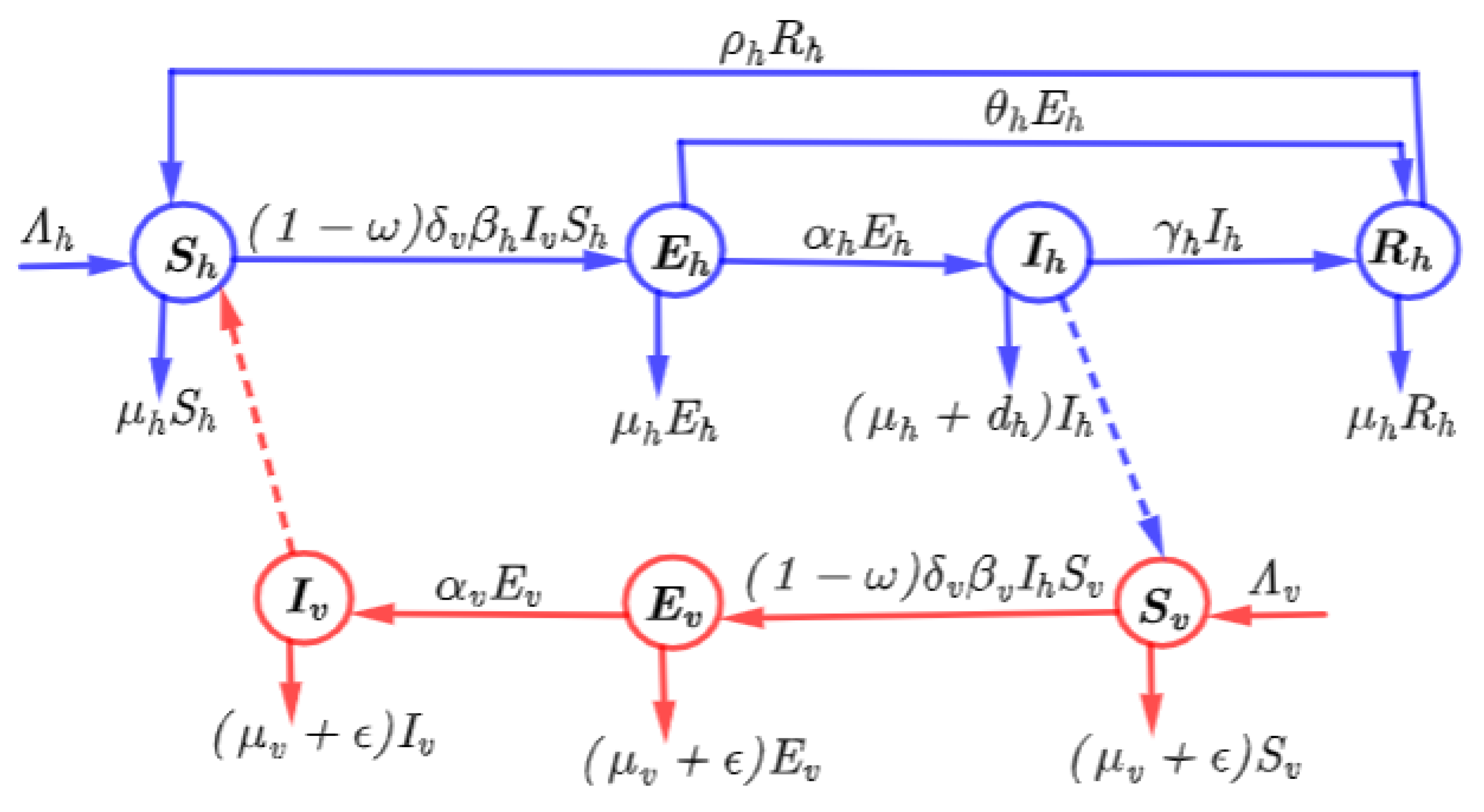
Figure 2.
Number of reported disease cases over 12 years in Zimbabwe
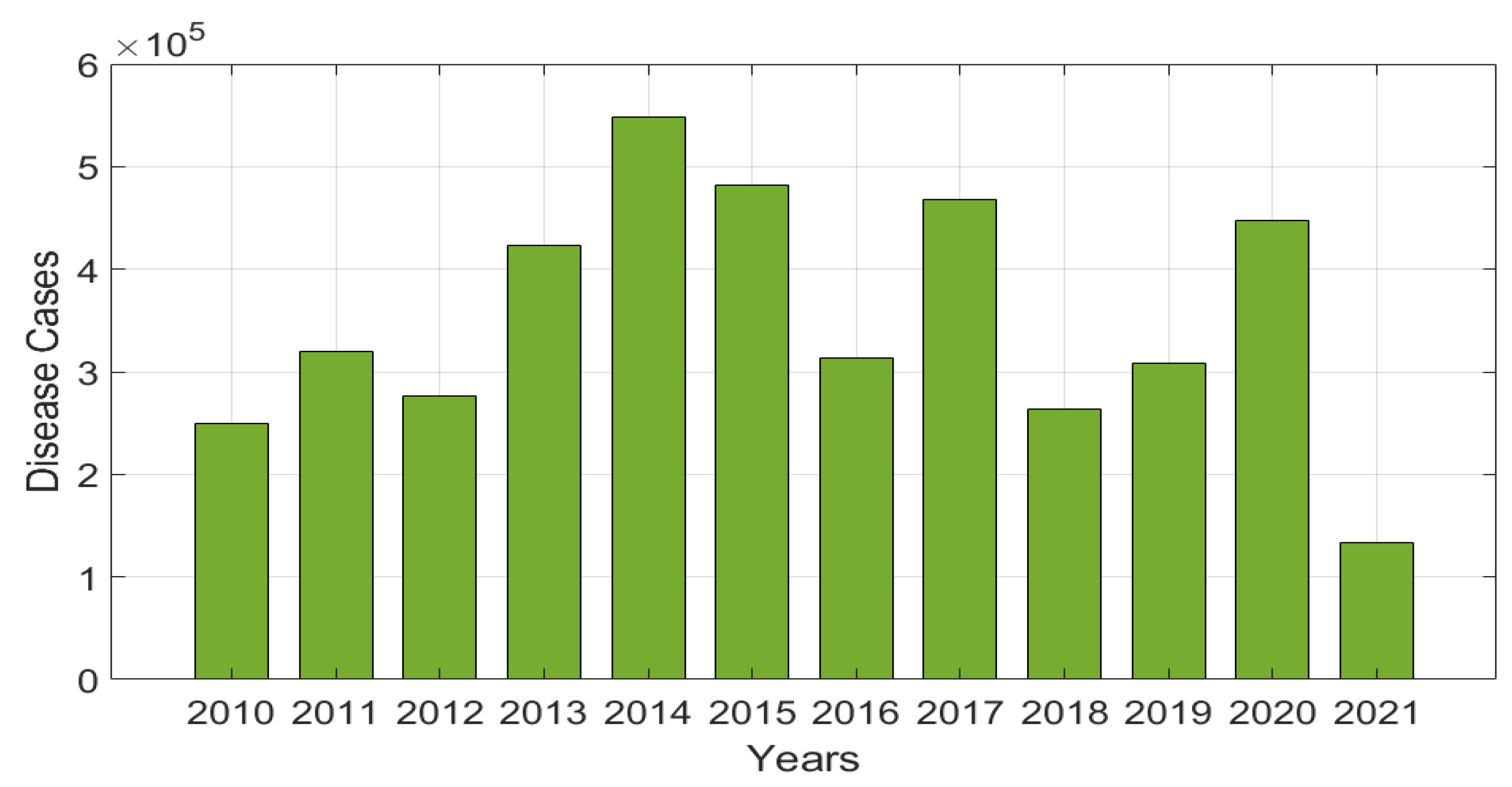
Figure 3.
(a) Model fit versus reported cases on malaria infections (b) Model fit versus reported malaria cases at and
Figure 3.
(a) Model fit versus reported cases on malaria infections (b) Model fit versus reported malaria cases at and
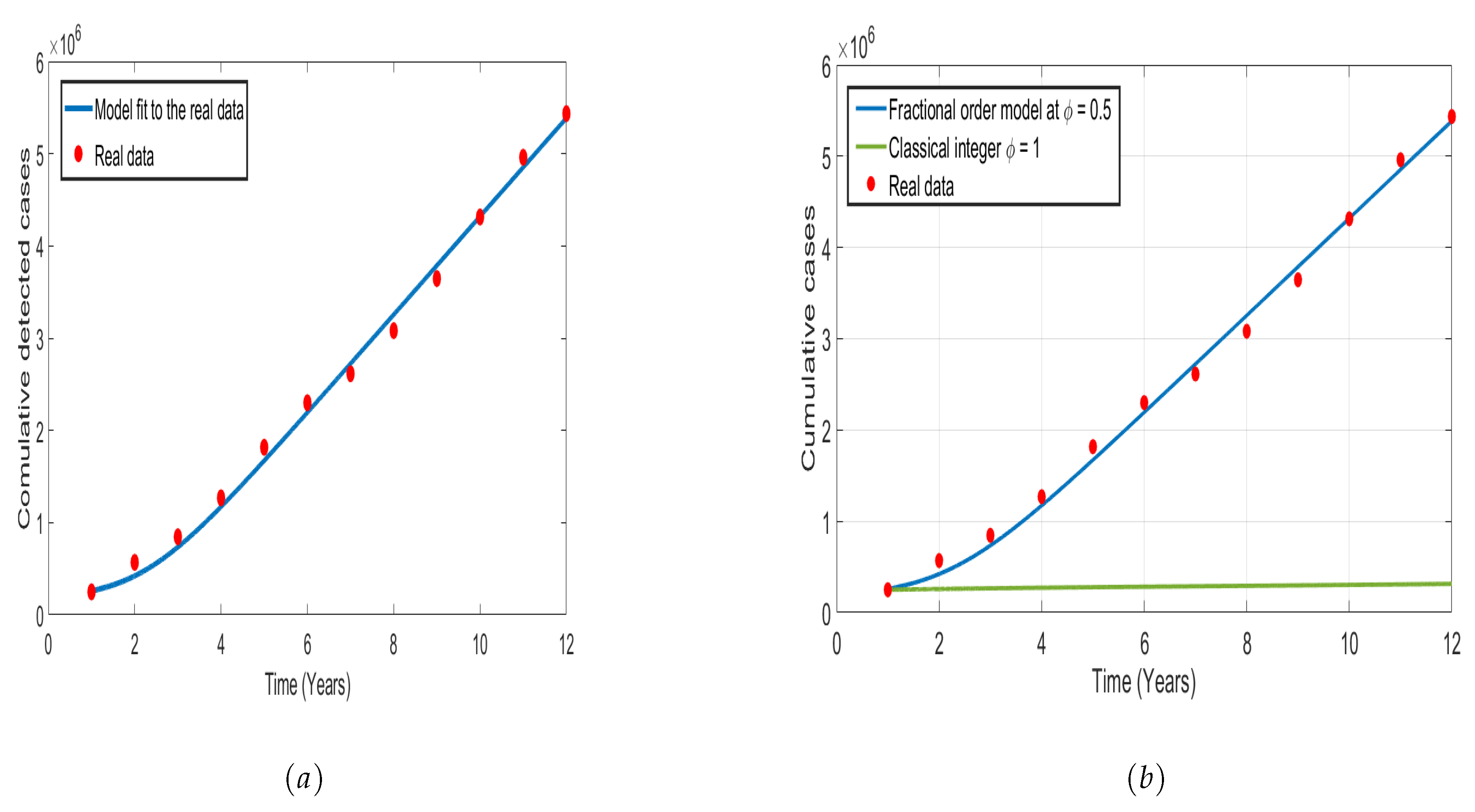
Figure 4.
Sensitivity analysis of to key model parameters
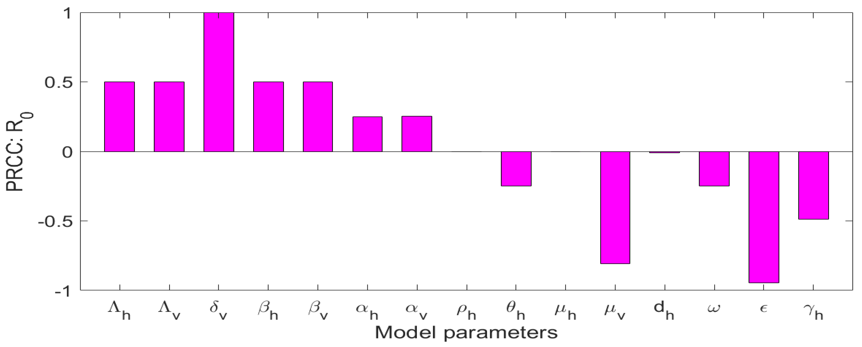
Figure 5.
Plot of global sensitivity analysis of the model (3) on () to the key parameters that affect the dynamics of the disease
Figure 5.
Plot of global sensitivity analysis of the model (3) on () to the key parameters that affect the dynamics of the disease
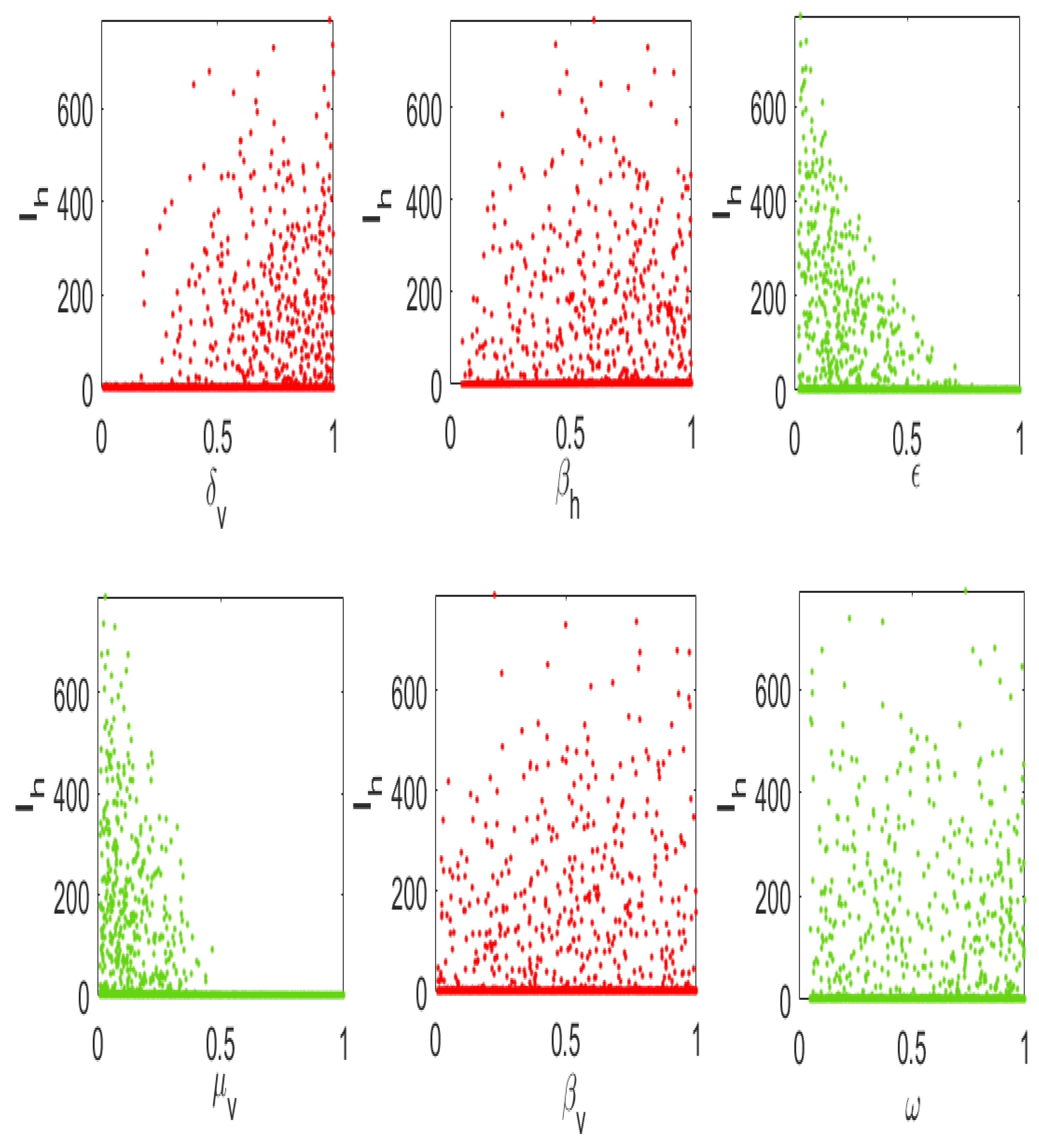
Figure 6.
Latin Hypercube sampling of to key model parameters, each parameter varied across the possible values
Figure 6.
Latin Hypercube sampling of to key model parameters, each parameter varied across the possible values
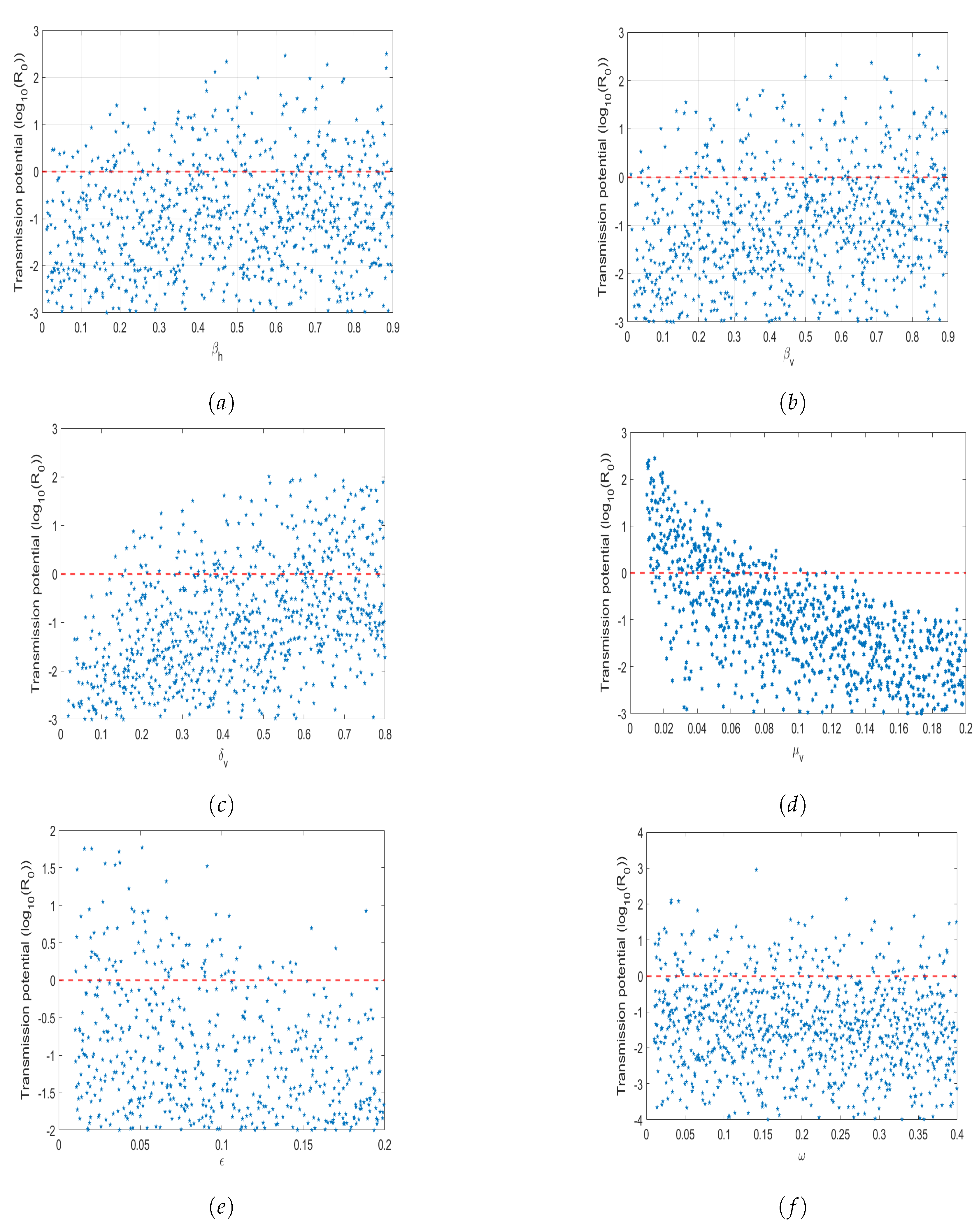
Figure 7.
Contour plots of as the function of use of prevention measures and vector biting rate
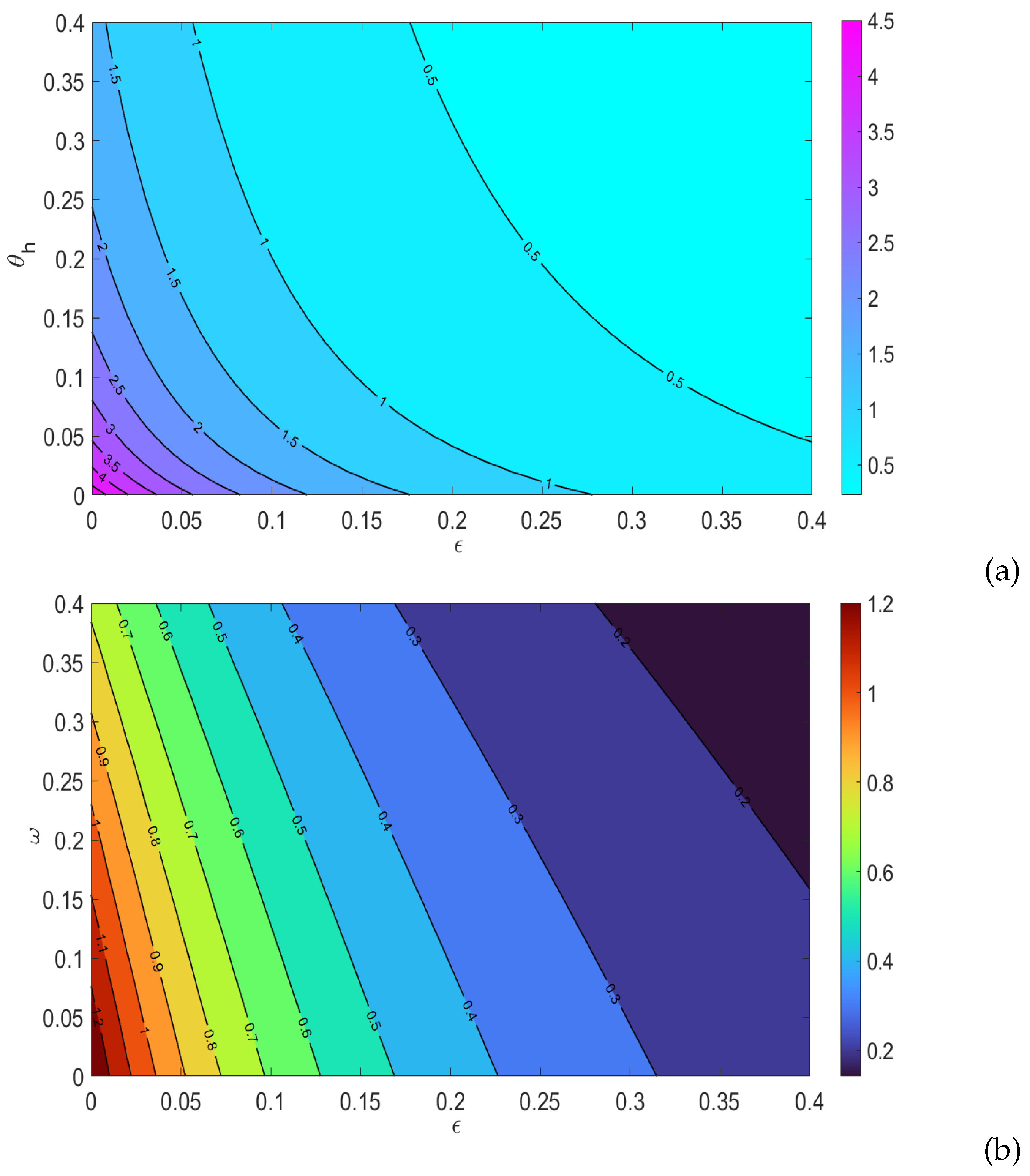
Figure 8.
Contour plots of variables against model parameters for (a) 20 days (b) 60 days.
Figure 9.
Simulation simulations of the model system (3) at with . Simulations were carried out using the parameter values shown in Table 1
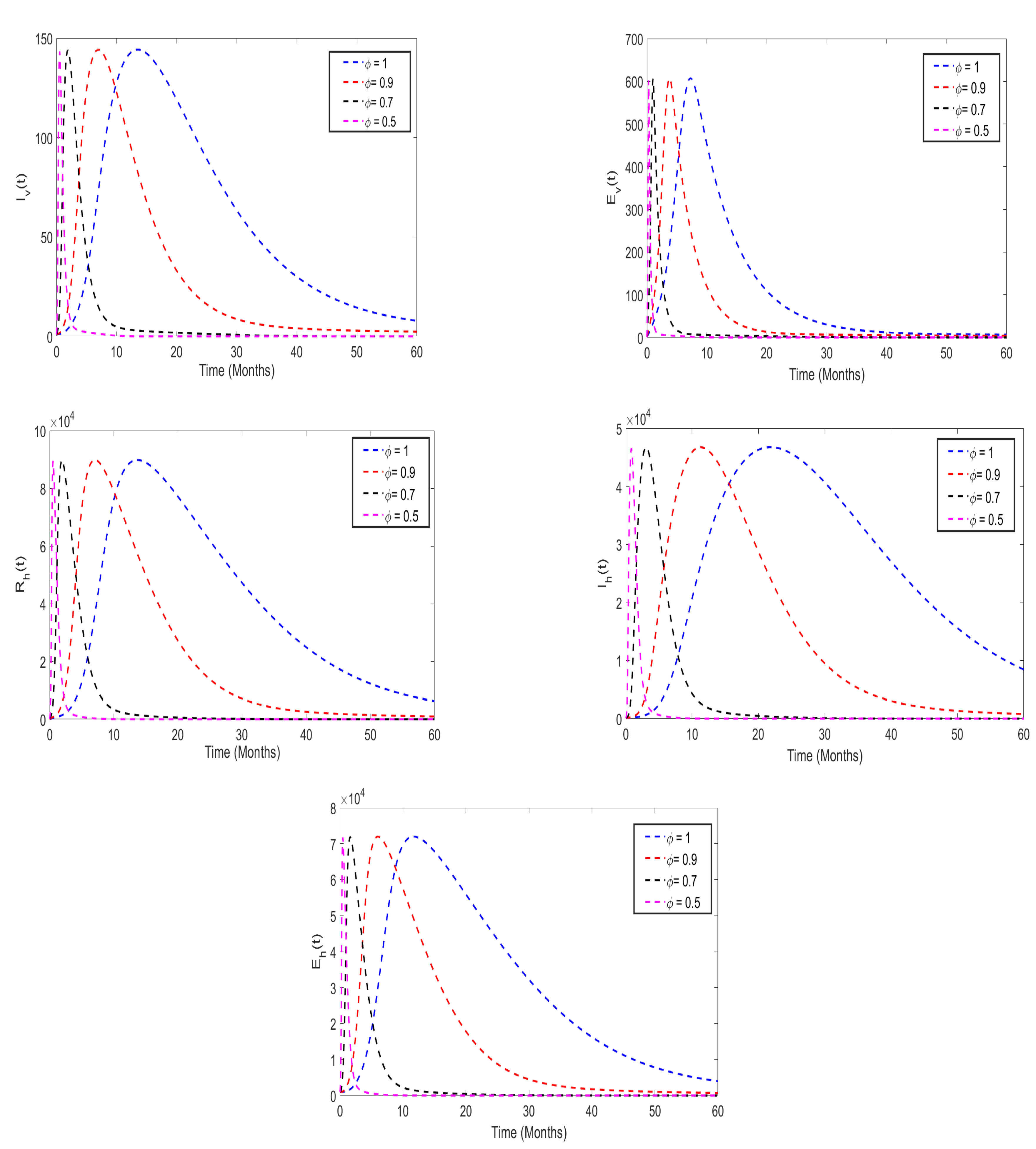
Figure 10.
Simulation simulations of the model system (3) at with . Simulations were carried out using the parameter values shown in table(Table 1)
Figure 11.
Simulation of the system (3) to investigate the effect of insecticide on the spread of malaria disease.
Figure 11.
Simulation of the system (3) to investigate the effect of insecticide on the spread of malaria disease.

Figure 12.
Effects of varying on reduction of new cases malaria infection generated in the population
Figure 12.
Effects of varying on reduction of new cases malaria infection generated in the population

Figure 13.
Simulation of the system (3) to investigate the effect of insecticide on the spread of malaria disease.
Figure 13.
Simulation of the system (3) to investigate the effect of insecticide on the spread of malaria disease.
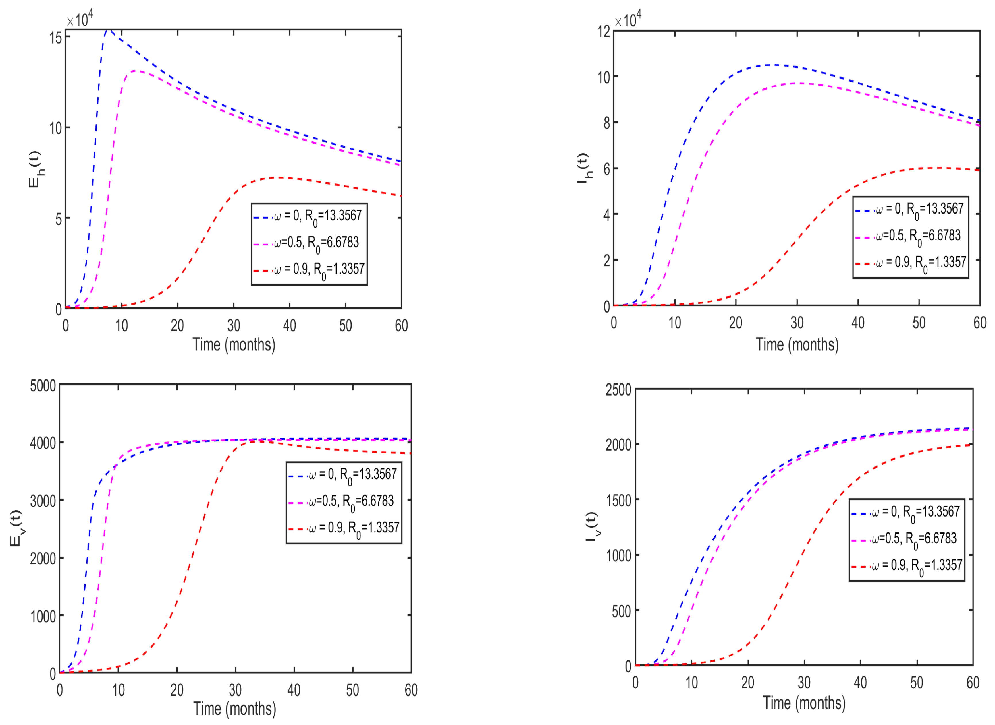
Figure 14.
Effects of varying on reduction of new malaria cases generated in the population
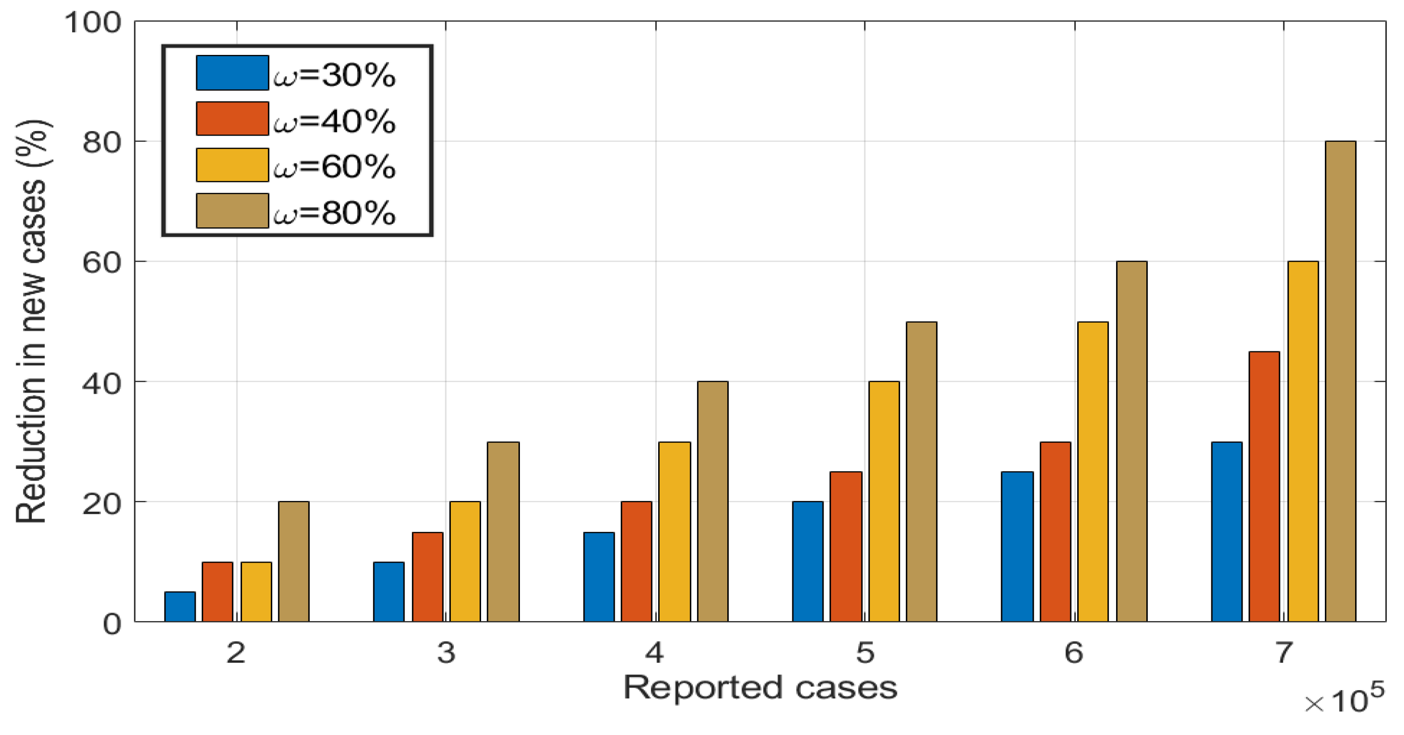

Table 1.
Definition of model parameters and values
| Symbol | Definition | Value | Units | Source |
|---|---|---|---|---|
| disease transmission from mosquito to human | 0.001 | [16,18] | ||
| disease transmission from human to mosquito | 0.0001 | [16,18] | ||
| natural mortality rate of human | [16,18] | |||
| natural mortality rate of vector | [16,18] | |||
| progression rate of human from incubation to infectious | 1/17 | [10,18] | ||
| progression rate of vector from incubation to infectious | 1/18 | [10,18] | ||
| progression rate of human from infectious to recovered class | [10] | |||
| new recruitment of human | 10 | [16,18] | ||
| new recruitment of Aedes mosquito | 50 | [10] | ||
| progression rate of exposed human to recovered class | fitted | |||
| Rate of use of insecticides | fitted | |||
| Proportion of human progress to infectious class | fitted | |||
| Rate of mosquito biting on human | 3 | [10] |
Disclaimer/Publisher’s Note: The statements, opinions and data contained in all publications are solely those of the individual author(s) and contributor(s) and not of MDPI and/or the editor(s). MDPI and/or the editor(s) disclaim responsibility for any injury to people or property resulting from any ideas, methods, instructions or products referred to in the content. |
© 2024 by the authors. Licensee MDPI, Basel, Switzerland. This article is an open access article distributed under the terms and conditions of the Creative Commons Attribution (CC BY) license (http://creativecommons.org/licenses/by/4.0/).
Copyright: This open access article is published under a Creative Commons CC BY 4.0 license, which permit the free download, distribution, and reuse, provided that the author and preprint are cited in any reuse.


