
Submitted:
29 October 2024
Posted:
30 October 2024
You are already at the latest version
Abstract
We show that analyzing archived and future multibeam backscatter and bathymetry data, in tandem with regional environmental parameters, can help identify polymetallic nodule fields in the world’s oceans. Extensive archived multibeam transit data through remote areas of the world’s oceans are available for data mining. New multibeam data will be made available through the Seabed 2030 Project. Uniformity of along and across track backscatter, backscatter intensity, angular response, water depth, nearby ground-truth data, and local slope, sedimentation rate, and seafloor age provide thresholds for discriminating areas permissive for nodule presence. A case study of this methodology is presented using archived multibeam data from a remote section of the South Pacific along the Foundation Seamounts between the Selkirk paleomicroplate and East Pacific Rise that were collected in 1997 during the Hotline cruise. The 12 kHz Simrad EM12 DUAL multibeam and the forementioned data strongly suggest a previously unknown nodule occurrence exists. Methods include comparing analyses using three different backscatter products to further determine if scanned backscatter products, rather than primary digital multibeam files can be used for analysis, and comparing results from using digitized 8-bit images, or 8-bit and decibel-value surfaces derived from the MB-SystemTM software. We show this expeditious analysis of broad areas of multibeam data could characterize benthic habitat types efficiently in remote deep ocean areas prior to more time consuming and expensive video and sample acquisition surveys. Additionally, utilizing software other than specialty sonar processing programs during this research explores how multibeam data products could be interrogated by a broader range of scientists and data users. Future mapping, video, and sampling cruises in this area would test our prediction and investigate how far it might extend to the north and south.
Keywords:
Multibeam echosounder
; Backscatter
; Polymetallic nodules
; Benthic habitat mapping
; Angular response
1. Introduction
Polymetallic nodules, also known as manganese nodules or ferromanganese (Fe-Mn) nodules, grow out of seawater or sediment pore water around any hard nucleus on deep-sea sediments and exist at various locations throughout the global ocean [1,2,3,4,5]. Individual nodules can range from <1 to 20 cm with most measuring 1-12 cm, and fields can cover hundreds of km2 with highly variable abundance [1,5,6,7]. Nodules serve as a deep-sea benthic habitat and are of economic interest owing to their metals content, as they are often enriched in Mn, Fe, Ni, Cu, Co, Ti and rare earth elements [1,3,5,8,9,10,11,12,13,14,15,16,17,18,19,20,21,22,23].
Existing analytical methods to identify prospective nodule areas include a review of oceanographic, geographic, geologic, and environmental parameters, supplemented with review of existing geological sample and seafloor photography records [14,24,25,26,27,28,29,30,31,32,33,34,35,36,37]. Principal component analysis of sediment characteristics can be incorporated with inputs for environmental values to facilitate mineral prospectivity mapping [26,38]. Mizell et al. (2022) note that areas conducive for nodule occurrence generally exhibit low bathymetric relief, low to moderate sedimentation rate and surface productivity, water depths near or below the carbonate compensation depth, and pre-Quaternary crustal age which typically implies the seafloor has subsided sufficiently to be below the CCD (carbonate compensation depth), and adequate time has passed for accretion of a nodule around a nucleus [34]. Nodule occurrences may not be contiguous within an area and often exhibit variable abundance and predominate physical characteristics, e.g., size and shape [39].
Acoustic backscatter data can aid in identifying nodules on the seafloor [9,11,18,40,41,42,43,44,45,46]. Oceanographic remote sensing data including multibeam bathymetry and backscatter data can be used to analyze prospective areas identified through initial desktop research. Previously collected, archived multibeam data are readily available for research, and additional multibeam data can be collected during follow up site investigations. However, the utility of using multibeam data collected during full speed transits for identifying nodule occurrence is not often considered nor discussed in the literature. Normally, exploratory surveys are planned with managed speed, sensor settings, regular sound velocity profile collection, etc., and may be undertaken with hull-mounted, towed, or AUV-mounted multibeam and side-scan systems [2,6,11,46,47,48,49,50,51,52,53,54,55,56,57,58,59,60,61,62,63,64,65,66,67].
The methodology described in this research is novel in that it further explores the use of transit multibeam backscatter and bathymetry for identifying potential nodule presence, with subsequent analysis of environmental parameters to evaluate whether the geographic context supports nodule formation, following the initial (Master’s thesis) work by Mussett (2023) [68]. This research also investigates the use of angular response diagrams derived for further classifying seafloor geology [6,46,69,70,71,72,73]. Angular response diagram generation undertaken in this research is based on pixel-value backscatter raster data. This provides an alternative to multibeam processing software methods for angular response analysis, as it requires only a backscatter raster product, and provides analysis based on averaged along-track pixel values rather than from a per-ping acoustic data file.
This research uses a case study based on real-time observations made during a transit where Simrad EM12 DUAL (12 kHz) multibeam bathymetry and backscatter data were collected on the Foundation-Hotline cruise aboard R/V Atalante, operated by IFREMER between Papeete (Tahiti) and Easter Island (Chile) in January and February 1997 with cruise objectives to map and date the Foundation Seamount chain up to the East Pacific Rise (EPR) [74,75]. No adjustments were made to gain settings during transit (coauthor D.F. Naar, personal communication, 2021).
The multibeam bathymetry data were used to generate a digital terrain model. The backscatter data were used both to generate digital surfaces via MB-SystemTM format identifier 76, as well as plot paper charts at sea during the cruise, which were digitized and georeferenced during this research [68,75,76]. The methods described herein are applicable for analyzing pixel-based outputs of backscatter data whether they are analog paper or digital.
The data coverage area includes an approximately 125 km long swath of homogenous high backscatter, hereafter referred to as Area A (Figure 1). Area A predominately consists of low relief seafloor and is distal from any known recent lava flows from any nearby seafloor spreading system or submarine volcanoes. This study analyzes multibeam bathymetry and backscatter data, auxiliary data regarding geographic parameters, and angular response of the backscatter to investigate if the high backscatter data in this area could be due to a large, previously uncharted and unexplored nodule field.
2. Observations
2.1. Transit Observations and Geological Setting
The ship transit investigated in this study trends approximately 102° and spans from approximately -32° latitude, -130° longitude to -39° latitude, -110° longitude. The transit crosses the Pacific plate from about ~25 Ma, across the EPR at 0 Ma, and out to ~1 Ma onto the Antarctic plate [77,78], and crosses a variety of seafloor terrain including abyssal hills, submarine volcanoes, lava flows, sedimented seafloor, and tectonic fabric and structures related to the Selkirk paleomicroplate (>20 Ma) in the far west [79].
Area A is not documented in literature as a known occurrence or region highly permissive for nodule formation [7,13,14,24,26,27,30,31,32,33,34,35,36,37,80,81,82], and is ~115 km north of suggested areas of low nodule abundance [26,81] and ~1700 km east from suggested area of high abundance [34]. However, there are two proximal ground truth sites that indicate nodules. One site (-36.33° latitude, -121.50° longitude) is <2 km from the northern extent of the data set and ~100 km to the northwest of Area A. This site provided a nodule sample recovered during sediment coring during the 14th cruise of R/V Dmitry Mendeleev in 1975 [83]. The other site from -35.22° latitude, -124.97° longitude, within the data set and ~450 km west of Area A consists of seafloor photos collected at core station 16 visited during the 24th cruise of USNS Eltanin in 1966. The core description indicates 2-5% micronodules in the upper 7 cm of core [84]. Seafloor photos from the station indicate abundant nodule coverage [68,85].
Water depths in the dataset range from 334 m (seamount summits) to 6630 m (failed rifts, trenches, fracture zones or pseudofaults related to the Selkirk paleomicroplate) [79]; the average seafloor depths from west to east along the transit (apart from the aforementioned shallow and deep features) rise from below to above the CCD, regionally estimated at approximately 4100 m [86].
2.2. Environmental Parameters Suitable for Nodule Formation
Seafloor below or near the CCD is considered a suitable environment for nodule formation [1,3,4,7,14,16,27]. Some nodule fields do exist above the CCD, e.g., Blake Plateau [4,87,88,89], Galicia Bank [90], the Pernambuco Plateau [91], and the South China Sea [92], and have different environmental constraints, which should be further reviewed to identify additional parameters that control their occurrence such as limitation of sedimentation resulting from strong near-bottom currents. This study focuses on nodule occurrence in deep water only.
Slope of the seafloor is also an important parameter for determining nodule presence from multibeam backscatter data. Areas delineated from hull-mounted, deep-water multibeam data exhibiting seafloor slope ≤7° can be considered conducive for nodule existence, and low slope environments, e.g., <10° further limit the impact of slope on acoustic backscatter [17,41].
Additionally, a very low sedimentation rate of 0.3 to <1 cm ka-1 is considered coincident with abundant nodule presence [1,13,24,93,94]. The sedimentation rate can be estimated using surface productivity as a proxy of POC (particulate organic carbon) flux to the seafloor [95,96], or by dividing sediment thickness [97] by seafloor age [78].
Seafloor age can also dictate whether an area is permissive for nodule occurrence. Newly created seafloor is often shallower than the local CCD, as is the case for the EPR and associated ridge structures included in this case study data. Additionally, time is required for newly created seafloor to subside to water depths below the CCD. Also, if an area is over a recent a recent lava flow, adequate time may not have lapsed for nodule accretion atop newly sedimented seafloor. Likewise, considering an estimated hydrogenetic radial nodule growth rate of 5 mm Ma-1 [1] to ~7 mm Ma-1 [83], a minimum of 2 Ma growth time is necessary for an accretion to reach a minimum 2 cm diameter, irrespective of nucleus size or mineral replacement of the nucleus. Hence, a 2 Ma minimum age can be considered a requirement for nodule formation where slow growth rate exists.
The influence of bottom water, dissolved oxygen concentrations in seawater, available sources of nuclei, dissolved metals content, and microtopography are not considered in this study owing to lack of data for this case study and a lack of agreement on influence of these parameters on abundant nodule presence.
2.3. Transit Areas Aligning with Prospective Nodule Characteristics
Along the transit near the EPR, all areas younger than 12 Ma are shallower than 4000 m, therefore above the estimated shallowest threshold for nodule presence, using a local CCD depth of ~4100 m [86] considered as a general ceiling for nodule occurrence in the Pacific [1,3,9]. Therefore, the youngest areas are neither old enough nor deep enough to satisfy requisite characteristics for nodule prospectivity. Most areas of older seafloor within the transit, including Area A, are not much deeper than 4000 m except the Kurchatov trough and the low slope seafloor immediately to its south.
The entirety of the data set (except very near the EPR) exhibits a sedimentation rate <1 cm ka-1 [78,97], therefore meeting the requisite sedimentation threshold described above.
Much of the data exhibit slopes less than the maximum threshold of 7° for nodule presence, though areas near the EPR and off-axis volcanic seamount chains, tectonic structure of the Kurchatov trough and Selkirk paleomicroplate, and isolated abyssal hill feature exhibit slopes greater than 7°. Both Area A and the area south of the Kurchatov trough consist of low slope seafloor along and across track.
3. Research Objectives
This research will attempt to predict whether a previously undescribed nodule occurrence exists within the data area, and whether it may relate to a larger nodule occurrence in the region. Methods will explore the utility of transit multibeam backscatter, firstly, and bathymetry, secondly for identifying potential nodule presence. Likewise, this research will address the suitability of backscatter products, rather than raw multibeam data, for identifying nodule presence on the deep seafloor. This will be done by comparing results from analysis of different outputs from the same original data set, e.g. 8-bit visualization of backscatter, a surface containing backscatter intensity values. This assessment will also inform whether the differing backscatter products produced from the same data, but with different software or methods, can provide for similar interpretations of seafloor characterization. Angular response diagrams from different visually apparent domains within the data will provide an additional basis against which to verify characterization based on backscatter value, bathymetry, and geologic parameters.
4. Materials and Methods
4.1 8-bit Graphic Paper Chart Analysis
During the cruise, 8-bit grey scale images with pixel values representing backscatter intensity were printed. For this research, these were digitally photographed at 300 dpi resolution using a Nikon D800. Images were merged into a single digital image with 8-bit pixel values using Adobe Photoshop 2022. This digital image was georeferenced using ESRI ArcMap 10.8, yielding an 80bit surface of 230 m X 230 m cell size [68]. As gain was not adjusted during data collection and visual observation of the paper charts does not indicate apparent along-track jumps in backscatter intensity, the relative backscatter values depicted by pixel values were used for analysis in [68].
Visually identifying seafloor domains identified in these images served as the first iteration of analysis. Observation identified areas of high, low, and variable backscatter. One homogenous area overlies the EPR, which is an area of known seafloor creation, and thus its pixel characteristics can be inferred to represent high backscatter values. Areas of homogenous, high backscatter values include the EPR, volcanic and abyssal hill structures extending distally from the EPR, and Area A. The Kurchatov trough and immediately adjacent areas exhibit variable backscatter.
Histogram equalization through a cumulative distribution function, and subsequent reclassification of the backscatter into a surface of 8 bins were undertaken as described in Mussett (2023) [68]. The reclassified backscatter data were then constrained by parameters conducive for nodule formation. This included elimination of pixels meeting the following parameters: <50% of the maximum backscatter value, shallower than the local CCD, where slope is >7°, where seafloor is younger than 2 Ma, and where sedimentation rate is ≥1 cm ka-1. This methodology identified areas within the data where nodules may be present.
4.2. Comparing 8-bit Graphic Paper Chart with Digital Backscatter Products
Digital multibeam data from the cruise were processed in MB-SystemTM to produce both an 8-bit backscatter surface (Graphic), and a surface containing intensity values on dB (decibel) basis (BS). These two surfaces and the 8-bit graphic paper chart (Scan) describe above are hereinafter referred to as the ‘three surfaces’. The three surfaces were compared using zonal statistics.
A 90 x 90 km fishnet grid was applied to delineate zones for general visualization of the data from the three surfaces. Trendlines of standard deviation, median, and mean for the three surfaces were created to illustrate similarities and differences between the three surfaces. Separately, a 4 x 4 km fishnet was applied to delineate zones to constrain the three surfaces to conducive nodule area based on bathymetry and geologic parameters. This included constraining the data to ≥1σ backscatter value to eliminate low backscatter zones, and further constraining the data to ≤-1σ standard deviation to eliminate high variability zones. These constraints emphasize areas where nodules may be present based on backscatter.
The final method for zonal statistical analysis included dividing the data coverage area into longitudinally equal zones of 1°. This segmented the data into 20 zones. The number of 4 x 4 km cells in each zone exhibiting low backscatter variability and high backscatter value were counted for each of the three surfaces to identify zones with a higher concentration of prospective nodule area. The 1° zones were then constrained by bathymetric and geologic parameters to include only areas with conducive environmental conditions for nodule presence. This constraint reduced the number of 1° zones from 20 to 14. The 1° zones with the highest concentration of 4 x 4 km cells, following the applied constraints described above, were identified as clusters where nodules may exist. These comparisons will test the similarity of results derived from the different methods of displaying and analyzing backscatter data.
4.3. Comparing Angular Response
Finally, angular response diagrams were generated from select sites representing visually different backscatter domains and different geographic locations. The diagrams were derived from cell values of the backscatter surface with pixel values in dB, and were not taken per-ping. Nadir position is estimated from nadir artifact position in the backscatter, and angle is estimated as a function of water depth, swath width, and across-track pixel position relative to nadir. Average backscatter value and diagram shape in terms of average departure from trendline intercept are recorded, and the qualitative profile shape was noted. These results are graphed against 15 kHz angular response backscatter data for a variety of substrate types as described in the High-Frequency Ocean Environmental Acoustic Models Handbook, hereinafter ‘handbook’ [98]. A qualitative comparison of angular response from the test case data and 12 kHz angular response from a survey area described by Yang et al. (2020) was also graphed [46]. The angular response data serve as another verification for use of backscatter data in delineating seafloor geology domains, and both the profile shape and across-track values relative to highest near-nadir values provide a basis for comparison with theoretical profile shapes attributable to different seafloor substrate.
5. Results
The three surfaces exhibit similar trends in their 90 x 90 km zonal statistics, indicating all three should generate similar results from a given analysis (Figure 2).
Producing zonal statistics for all three surfaces on a 4 x 4 km zonal basis (normalizing resolution to 16 km2 cells, hereinafter ‘cells’) allowed for cluster analysis to be undertaken and the surfaces to be compared. This was achieved by further binning the surfaces to bins of 1° longitude width (Figure 3). Constraining the three surfaces to only cells exhibiting high backscatter values identifies areas of low seafloor acoustic absorption e.g. hard substrate including crusts, nodules, exposed basalt, etc.; additionally constraining the surfaces to only include cells with low backscatter standard deviation (σ) further identifies areas of homogenous backscatter intensity. When an area is shown to exhibit high backscatter values and high backscatter homogeneity, it is inferred as a uniform or semi-uniform expanse of relatively hard seafloor substrate.
Counting the percentage of total cells present in each 1° bin for each respective surface emphasizes clusters of strong, homogenous backscatter. This also allows for differences between the three surfaces to be examined. The results for all three surfaces are similar, with 1° zones 8, corresponding to the Kurchatov trough area, 11, corresponding to Area A, and 19 and 20, corresponding to the EPR emphasized as clusters of high, homogeneous backscatter (Figure 4 and Figure 5; Table 1). However, while the two surfaces created via MB-SystemTM align very closely (R = 0.998), the scanned surface correlates well but not as closely (R = 0.912), exhibiting higher stack line peaks for clusters in Zones 10, 11 and 12 (Area A and adjacent), and a lower peak in Zone 8 (Kurchatov trough).
Further constraining the high backscatter, low σ filtered data to only those geographic areas in the data >2 Ma old and accumulating sediment at a rate of 0.3 to <1 cm ka-1, and also shown by bathymetry data to be deeper than the local CCD and exhibit a slope ≤7° identifies areas most conducive for nodule presence. The three surfaces all identify similar areas within the data exhibiting homogenous, high backscatter which, based on bathymetric and geologic context, are attributable to nodule presence. These areas include the Kurchatov trough area (Zone 8) and Area A (Zone 11, with lesser clusters in the adjacent Zones 10 and 12); the EPR area is excluded based on age and water depth. Similarly to the comparison of the cell distributions prior to filtering by slope, depth, sedimentation rate and age, the two surfaces created via MB-SystemTM align very closely (R = 0.999), and the scanned surface correlates well but not as closely (R = 0.941 between ‘backscatter’ and ‘scan’ surfaces, and R = 0.943 between ‘graphic’ and ‘scan’ surfaces). For all 3 surfaces higher cluster peaks exist in Zones 10, 11 and 12 (Area A and adjacent), with a lower peak in Zone 8 (Kurchatov trough) (Figure 6 and Figure 7; Table 2).
Angular response data from select geographic locations indicate a difference in seafloor substrate for sections of the data. This is determined by both the mean across-track backscatter intensity, and profile shape of the angular response diagram. These locations are shown in Figure 8 and described in Table 3. Figure 9 depicts the angular response of the across-track sites within the data. Figure 10 depicts the same as well as modelled profiles for 15 kHz sonar for a range of substrate types as described in the handbook [98], and Figure 11 depicts the same with an additional overlay of angular response at 12 kHz by substrate type, including nodules of ~20 kg/m2 and ~40 kg/m2 abundance observed at a site in the western Pacific Ocean adapted from Yang et al. (2020) [46].
Sites within the data where across-track angular response diagrams were generated from the backscatter surface generated in MB-SystemTM with cell values in dB (Table 3). The absolute average difference between the diagram trendline and nadir intercept was used as a marker of general flatness of the profile in terms of the range of backscatter values about the trendline intercept. Site 5, corresponding to Area A exhibited the lowest variability. Site 7, corresponding to the area south of the Kurchatov trough exhibited the highest variability. Sites 5, 6, 7, and 9 are the only sites >1σ difference of intercept to backscatter across track, indicating these are significantly higher or lower in terms of their profile flatness. Sites 1 and 5 exhibit the highest mean backscatter values. The high mean backscatter and flat profile of Site 5 align with an expected nodule profile as shown in Figure 11, adapted from Yang et al. (2020) [46].
6. Discussion
Analysis of the multibeam bathymetry and backscatter data together with the environmental data predict nodule occurrences both in Area A, and south of the Kurchatov trough. Across-track angular response diagrams qualitatively reinforce the characterization of nodule presence in Area A (Site 5), while suggesting a different type of substrate, or more variable seafloor geology may exist south of the Kurchatov trough (Site 7). However, the area analyzed for angular response south of the Kurchatov trough only overlaps potential nodule areas from ~30° to ~70° angle of incidence (Figure 7 and Figure 8). For this section of the Kurchatov trough area (Site 7) angular response diagram the angular response closely aligns with the respective sections of angular response diagrams of the EPR (Site 1) and Area A (Site 5), indicating nodule presence only in this section of the data area analyzed for Site 7. It must be noted the angular response diagrams were generated from the backscatter raster, and were not taken per-ping.
The extent to which multibeam data editing may have impacted the results is not evident when working only with raster data. However, this methodology may provide a more readily attainable means for assessing angular response by scientists without access to digital multibeam data or specific software needed for generating angular response diagrams. However, this method requires additional effort and inherent imprecision for matching a wide swath from a hull-mounted multibeam system operated in deep water with the most likely average seafloor type in a specific location in the data; if the wide swath encounters an area of apparent variable backscatter, the angular response profile may not match closely with a modeled profile. Without built-in capability afforded by specialized software, interpretation can prove more challenging for an investigator to accurately, and consistently, determine. Ideally, calibrated backscatter data can be acquired with a respective system and used as a benchmark. Comparative analysis undertaken in this research relied on profiles described in both the handbook [98], which did not provide a 12 kHz model output, as well as by Yang et al. (2020) [46], which considered data collected in the same ocean and at the same frequency but with a multibeam system not necessarily intended to be used as a calibrated benchmark to compare with other backscatter data. However, this research indicates the use of angular response diagrams as an evaluative tool work well as a complement to analysis undertaken with bathymetry and backscatter surfaces.
During this research, similar results were achieved regardless of which of the three surfaces were used, though trends were more subdued in the scanned chart. The scanned chart allows for data analysis but digital products derived in MB-SystemTM provide greater data density, which may result in accentuated trends in pixel distribution graphs. Similarities between the three surfaces may be accentuated owing to processing undertaken during and following the cruise, which may have included treatment in the contemporaneous Simrad or IFREMER acquisition and processing software suites (e.g., CARAIBES ©). Comparing results from additional data sets and products, as well as products produced from additional software suites may offer future opportunity to address the research objective of whether differing backscatter products produced from the same data, but with different software or methods, can provide for similar interpretations of seafloor characterization.
This study suggests backscatter products such as raster surfaces provide a suitable basis for evaluating prospective nodule areas and delineating seafloor substrate types; while assessment relying on raw multibeam data may compliment or refine results based solely on backscatter products, the adaptability of backscatter products in software other than specialized multibeam software may afford more opportunity to a broader range of scientists and persons interested in characterizing seafloor geology.
Explanations for high backscatter intensity other than nodule presence include presence of abyssal hill outcrops, recent lava flows, or polymetallic crusts. However, the geomorphology of both Area A and the area south of the Kurchatov trough do not indicate the characteristic dendritic patterns of lava flows or sharp contrasts with older sedimented seafloor (e.g., Hagen et al., 1990) [99]. Polymetallic crust presence, e.g., Fe-Mn coating on exposed igneous basement may be present throughout this general area of the transit, but this coating is not expected to be a predominate feature of Area A, because unlike nodules, flat crusted seafloor would be buried by sediment in this location. Likewise, the differences in angular responses and the broad areas of high, homogenous backscatter (Figure 9, Figure 10 and Figure 11) would be best explained by a large nodule field.
Future ground-truth data collection will be needed to test this prediction and validate the applicability of this method in detecting nodule fields. Models based on remote sensing data can be trained with inputs of empirical data to establish nodule domains, as well as geological domains of different seafloor type. Differentiating seafloor substrate types will assist with marine spatial planning, as domain types, spatial extents of individual domains, and benthic habitats can be more precisely defined. This may facilitate marine spatial planning initiatives and fulfillment of objectives such as the protection and conservation designation of 30% of marine area by 2030 as stated in the Kunming-Montreal Global Biodiversity Framework, as well as support ongoing management of marine mineral resources, e.g., the International Seabed Authority [100,100,101,101,102].
The whole of this case study data exist in international waters, in an area with seabed resources administered by the United Nations. Area A accounts for ~3,000 km2 of seafloor, and the potential nodule area south of the Kurchatov trough accounts for ~1,000 km2 of seafloor. Estimated area of seafloor prospective for abundant nodules in the Pacific Ocean is ~28,000,000 km2 from 9 areas, ranging from ~350,000 km2 to ~8,000,000 km2 [34]. Should Area A and the surrounding region be confirmed to contain abundant nodule fields, this would contribute to estimates of Pacific seafloor containing nodules and support efforts to classify benthic habitat domains throughout the Pacific. Similar high resolution data are scarce in the region; low-resolution bathymetric estimates and application of filters for environmental parameters conducive for nodule presence suggest the occurrences indicated in the case study data may be part of a much larger occurrence. As more of the world’s oceans are mapped in high resolution, new data may show this area as a continuance of known occurrences in the southern Pacific Ocean, or as a unique contiguous field unconnected to known occurrences. Future multibeam data collection, particularly adjacent to the data boundary to the south and east of the Kurchatov trough area, as well as north and south of Area A would enable such an assessment.
7. Conclusions
Analysis indicates Area A and the area south of the Kurchatov trough contain polymetallic nodule occurrences. This is based on the respective data characterization of homogenous, high backscatter value, and application of bathymetric and geologic context. Zonal analysis of the data indicates a higher concentration of 16 km2 cells exhibiting high backscatter values and low heterogeneity within Area A than elsewhere in the data. This is true whether or not the data are constrained to areas conducive for nodule formation. The zone including the Kurchatov trough exhibits the second highest concentration of such cells when constraining to areas conducive for nodule formation, while the EPR exhibits the second highest concentration of such cells when constraints for nodule formation are not applied. The scanned paper chart contains a higher proportion of such cells in Area A than do the MB-SystemTM backscatter products; likewise, clusters of such cells are less apparent in the scanned paper chart results when mapping these data, perhaps owing to the higher data density of MB-SystemTM products.
A relative seafloor valley slightly below the CCD exists in and immediately adjacent to Area A, while low-slope seafloor of ~4500 m water depth exists to the south of the Kurchatov trough. Results suggest smaller areas within the data also may contain nodules, though proximity to tectonic structures limits their expanse compared to Area A and the plain south of the Kurchatov trough. Qualitative assessment of angular response diagrams generated from select locations throughout the data indicate geological characteristics differ, and reinforce the interpretation of nodule presence where bathymetry, backscatter value, and environmental parameters suggest. Although ground-truth sample data are required to validate the characteristics of seafloor geological domains, this research strongly suggests that transit multibeam bathymetry and backscatter data, including angular response, can be used with geologic and environmental data, prior to ground-truth data collection, to predict areas of deep seafloor likely to contain polymetallic nodules.
The primary variables to identify areas likely to contain polymetallic nodules are homogeneous, strong multibeam backscatter data in areas of seafloor older than 2 Ma that are deeper than the CCD, subject to sedimentation rates of 3 to <10 mm ka-1, and with an overall seafloor slope ≤7o. Based on this proposed method we predict evidence from a single multibeam transit indicates two areas of respectively ~3,000 km2 and ~1,000 km2 in water depths >4,000 m contain nodule occurrences. These locations are limited to the extent of the data. Future use of similar methods may be used with low resolution bathymetric estimates of adjacent areas to identify whether a much more expansive occurrence may exist in the region, though angular response analysis would not be possible and results would only be indirectly comparable owing to poorer bathymetric resolution. Future work may also include a data mining exercise to locate geological samples coincident with data collected using the same multibeam system in comparable water depths; this would allow for an additional case study, and provide an empirical basis for interpretating angular response diagrams generated in this study.
Lastly, considering the vast amount of archived multibeam transit data through remote areas of the world’s oceans and new multibeam data expected from the Seabed 2030 Project [103,104,105,106,107], we propose that this type of first-order analysis could be useful as a cost-effective, desk-based analytical method for determining other potential nodule fields using a specific set of variables starting with multibeam backscatter data exhibiting high values and homogeneity (along and across track), geomorphology from multibeam bathymetry, environmental parameters conducive for nodule formation, and angular response profiles fitting a shape and intensity representing a high impedance, high rugosity seafloor. This proposed method could help prioritize future exploration activities including transit planning to or from focused survey areas, and can assist scientists and regulators in estimating marine ecological and mineral resources. Additional industrial applications for characterizing seafloor geology with these methods include cable route surveys, locating seamounts or other features, which could pose a navigation hazard, and identifying types of seafloor habitats.
Funding
This research was funded in part by the NOAA-USF Center for Ocean Mapping and Innovative Technologies (COMIT), and the University of South Florida College of Marine Science.
Acknowledgments
This work has benefited from funding and discussions within the NOAA-USF Center for Ocean Mapping and Innovative Technologies (COMIT). Additional details related to this work can be found within the online thesis (Mussett, 2023).
Conflicts of Interest
The authors declare no conflicts of interest. The funders had no role in the design of the study; in the collection, analyses, or interpretation of data; in the writing of the manuscript; or in the decision to publish the results.
References
- Hein JR, Koschinsky A. Deep-ocean ferromanganese crusts and nodules. In: Treatise on geochemistry [Internet]. Second. Elsevier; 2014. p. 273–91. Available from: https://pubs.usgs.gov/publication/70046853.
- Kodagali VN, Chakraborty B. Multibeam echosounder pseudo sidescan images as a tool for manganese nodule exploration. In: Proceedings of the third (1999) ocean mining symposium. 1999. p. 97–104.
- Kuhn T, Wegorzewski A, Rühlemann C, Vink A. Composition, Formation, and Occurrence of Polymetallic Nodules. In: Sharma R, editor. Deep-Sea Mining: Resource Potential, Technical and Environmental Considerations [Internet]. Cham: Springer International Publishing; 2017. p. 23–63. Available from. [CrossRef]
- Mero, JL. The Mineral Resources of the Sea. Vol. 1. Elsevier; 1965. 1–311 p.
- Verlaan PA, Cronan DS. Origin and variability of resource-grade marine ferromanganese nodules and crusts in the Pacific Ocean: A review of biogeochemical and physical controls. Geochemistry. 2022 Apr;82(1):125741.
- Chunhui T, Xiaobing J, Aifei B, Hongxing L, Xianming D, Jianping Z, et al. Estimation of Manganese Nodule Coverage Using Multi-Beam Amplitude Data. Marine Georesources and Geotechnology. 2015 Jul;33(4):288–93.
- Glasby, GP. Marine Manganese Deposits (Elsevier oceanography series ; 15). Glasby GP, editor. Vol. 15. Elsevier North-Holland Inc.; 1977. 1–523 p.
- Cronan, DS. Deep Sea Minerals: David Cronan on the fall and rise of mining the ocean depths. Geoscientist. 2015;25(8):10–5.
- Kuhn T, Uhlenkott K, Vink A, Rühlemann C, Martinez Arbizu P. Chapter 58 - Manganese nodule fields from the Northeast Pacific as benthic habitats. In: Harris PT, Baker E, editors. Seafloor Geomorphology as Benthic Habitat (Second Edition) [Internet]. Elsevier; 2020. p. 933–47. Available from: https://www.sciencedirect.com/science/article/pii/B9780128149607000580.
- Abramowski T, Stoyanova V. Deep-sea polymetallic nodules: renewed interest as resources for environmentally sustainable development. In: 12th International Multidisciplinary Scientific GeoConference SGEM 2012 [Internet]. 2012. p. 515–21. Available from: https://www.researchgate.net/publication/255566122.
- Alevizos E, Schoening T, Koeser K, Snellen M, Greinert J. Quantification of the fine-scale distribution of Mn nodules: insights from AUV multi-beam and optical imagery data fusion. Biogeosciences Discussions [Internet]. 2018; Available from:. [CrossRef]
- Alvarenga RAF, Préat N, Duhayon C, Dewulf J. Prospective life cycle assessment of metal commodities obtained from deep-sea polymetallic nodules. Journal of Cleaner Production. 2022;330:129884.
- Glasby GP, Li J, Sun Z. Deep-Sea Nodules and Co-rich Mn Crusts. Marine Georesources and Geotechnology. 2015 Jan;33(1):72–8.
- Hein JR, Spinardi F, Tawake A, Mizell K, Thorburn D. Hein-1 42nd Underwater Mining Institute · 21-29. JICA/MMAJ. Cronan; 2013.
- Hein JR, Spinardi F, Okamoto N, Mizell K, Thorburn D, Tawake A. Critical metals in manganese nodules from the Cook Islands EEZ, abundances and distributions. Ore Geology Reviews. 2015 Jul;68:97–116.
- Hein JR, Koschinsky A, Kuhn T. Deep-ocean polymetallic nodules as a resource for critical materials. Nature Reviews Earth & Environment. 2020 Mar 1;1(3):158–69.
- Kuhn T, Rühlemann C. Exploration of polymetallic nodules and resource assessment: A case study from the german contract area in the clarion-clipperton zone of the tropical northeast pacific. Minerals. 2021 Jun;11(6).
- Ma Y, Magnuson AH, Varadan VK, Varadan VV. Acoustic response of manganese nodule deposits. Geophysics. 1986;51(3):689–98.
- Petersen S, Krätschell A, Augustin N, Jamieson J, Hein JR, Hannington MD. News from the seabed – Geological characteristics and resource potential of deep-sea mineral resources. Marine Policy. 2016 Mar;70:175–87.
- Purser A, Marcon Y, Hoving HJT, Vecchione M, Piatkowski U, Eason D, et al. Association of deep-sea incirrate octopods with manganese crusts and nodule fields in the Pacific Ocean. Current Biology. 2016;26(24):R1268–9.
- Rühlemann C, Kuhn T, Wiedicke M, Kasten S, Mewes K, Picard A. Current Status of Manganese Nodule Exploration in the German License Area [Internet]. 2011. Available from: www.isope.
- Vanreusel A, Hilario A, Ribeiro PA, Menot L, Arbizu PM. Threatened by mining, polymetallic nodules are required to preserve abyssal epifauna. Scientific Reports. 2016;6(1):26808.
- Wang X, Müller WEG. Marine biominerals: perspectives and challenges for polymetallic nodules and crusts. Trends in Biotechnology. 2009;27(6):375–83.
- Hein JR, Mizell K. Chapter 8 Deep-Ocean Polymetallic Nodules and Cobalt-Rich Ferromanganese Crusts in the Global Ocean: New Sources for Critical Metals. In Leiden, The Netherlands: Brill | Nijhoff; 2022. p. 177–97. Available from: https://brill.com/view/book/edcoll/9789004507388/BP000021.
- Baturin, GN. Mineral Resources of the Sea. Lithology and Mineral Resources. 2000;35(5):399–424.
- Dutkiewicz A, Judge A, Müller RD. Environmental predictors of deep-sea polymetallic nodule occurrence in the global ocean. Geology. 2020;48(3):293–7.
- Exon NF, Cronan DS, Colwell JB. New developments in manganese nodule prospects, with emphasis on the Australasian region. In: The Australasian institute of mining and metallurgy. 1990. p. 363–71.
- Glasby GP, Stoffers P, Sioulas A, Thijssen T, Friedrich G. Manganese nodule formation in the Pacific Ocean: a general theory. Geo-Marine Letters. 1982;2:47–53.
- Ko Y, Lee S, Kim J, Kim KH, Jung MS. Relationship between Mn nodule abundance and other geological factors in the Northeastern Pacific: Application of GIS and probability method. Ocean Science Journal. 2006 Sep;41:149–61.
- Lusty PAJ, Murton BJ. Deep-ocean mineral deposits: Metal resources and windows into earth processes. Elements. 2018 Oct;14(5):301–6.
- Mckelvey VE. USGS bulletin b1689A: Subsea Mineral Resources [Internet]. USGS; 1986. Available from: https://pubs.er.usgs.gov/publication/b1689A.
- Mckelvey VE, Wright NA, Bowen RW. Analysis of the World Distribution of Metal-Rich Subsea Manganese Nodules. 1983.
- McKelvey VE, Wang FFH. World subsea mineral resources. United States Geological Survey; 1969 p. 17.
- Mizell K, Hein JR, Au M, Gartman A. Estimates of Metals Contained in Abyssal Manganese Nodules and Ferromanganese Crusts in the Global Ocean Based on Regional Variations and Genetic Types of Nodules. In: Sharma R, editor. Perspectives on Deep-Sea Mining: Sustainability, Technology, Environmental Policy and Management [Internet]. Cham: Springer International Publishing; 2022. p. 53–80. Available from. [CrossRef]
- Murton, BJ. A Global Review of Non-living Resources on the Extended Continental Shelf. 2000; Available from: www.un.org/Depts/los/tempclcs/docs/clcs/.
- Rona, PA. Resources of the Sea Floor. Science. 2003 Jan 31;299(5607):673–4.
- Rona, PA. The changing vision of marine minerals. Ore Geology Reviews. 2008 Jun;33(3–4):618–66.
- Kaufmann, M. The Hunt for Deep-Sea Minerals – Identifying and Analysing Formation Areas of Marine Minerals [[Unpublished]]. University of Exeter; 2020.
- Cronan, DS. Underwater Minerals [Internet]. Academic Press; 1980. 1–392 p. Available from: https://archive.org/details/underwaterminera0000cron/page/n7/mode/2up?
- Moustier C, de. Inference of manganese nodule coverage from Sea Beam acoustic backscattering data. Geophysics. 1985;50(6):989–1001.
- Machida S, Sato T, Yasukawa K, Nakamura K, Iijima K, Nozaki T, et al. Visualisation method for the broad distribution of seafloor ferromanganese deposits. Marine Georesources and Geotechnology. 2021;39(3):267–79.
- Masson DG, Scanlon KM. Comment on the mapping of iron-manganese nodule fields using reconnaissance sonars such as GLORIA. Geo-Marine Letters. 1993 Dec;13(4):244–7.
- Scanlon KM, Masson DG. Ge0-Marine Letters Fe-Mn Nodule Field Indicated by GLORIA, North of the Puerto Rico Trench. Vol. 12. 1992 p. 208–13.
- Weydert MMP. Measurements of the acoustic backscatter of selected areas of the deep seafloor and some implications for the assessment of manganese nodule resources. Journal of the Acoustical Society of America. 1990;88(1):350–66.
- Weydert MMP. Measurements of the acoustic backscatter of manganese nodules. Journal of the Acoustical Society of America. 1985;78(6):2115–21.
- Yang Y, He G, Ma J, Yu Z, Yao H, Deng X, et al. Acoustic quantitative analysis of ferromanganese nodules and cobalt-rich crusts distribution areas using EM122 multibeam backscatter data from deep-sea basin to seamount in Western Pacific Ocean. Deep-Sea Research Part I: Oceanographic Research Papers. 2020 Jul;161.
- Brown CJ, Beaudoin J, Brissette M, Gazzola V. Multispectral multibeam echo sounder backscatter as a tool for improved seafloor characterization. Geosciences (Switzerland). 2019 Mar;9(3).
- Alevizos E, Huvenne VAI, Schoening T, Simon-Lledó E, Robert K, Jones DOB. Linkages between sediment thickness, geomorphology and Mn nodule occurrence: New evidence from AUV geophysical mapping in the Clarion-Clipperton Zone. Deep-Sea Research Part I: Oceanographic Research Papers. 2022 Jan;179.
- Chakraborty B, Pathak D, Sudhakar M, Raju YS. Determination of nodule coverage parameters using multibeam normal incidence echo characteristics: A study in the Indian Ocean. Marine Georesources and Geotechnology. 1997 Jan;15(1):33–48.
- Chakraborty B, Kodagali V. Characterizing Indian Ocean manganese nodule-bearing seafloor using multi-beam angular backscatter. Geo-Marine Letters. 2004 Feb;24(1):8–13.
- Cui X, Liu H, Fan M, Ai B, Ma D, Yang F. Seafloor habitat mapping using multibeam bathymetric and backscatter intensity multi-features SVM classification framework. Applied Acoustics. 2021 Mar;174.
- Dewolfe J, Ling P. NI 43-101 technical report for the NORI Clarion-Clipperton Zone project, Pacific Ocean. 2018.
- Flentje W, Lee SE, Virnovskaia A, Wang S, Zabeen S, Shenoi R, et al. Polymetallic nodule mining: innovative concepts for commercialisation. In 2012.
- Gazis IZ, Schoening T, Alevizos E, Greinert J. Quantitative mapping and predictive modeling of Mn nodules’ distribution from hydroacoustic and optical AUV data linked by random forests machine learning. Biogeosciences. 2018 Dec;15(23):7347–77.
- Huggett QJ, Somers ML. Possibilities of Using the GLORIA System for Manganese Nodule Assessment. Marine Geophysical Researches. 1988;9:255–64.
- Lee SH, Kim KH. Side-scan sonar charateristics and manganese nodule abundance in the Clarion-Clipperton fracture zones, NE equatorial Pacific. Marine Georesources and Geotechnology. 2004 Jan;22(1–2):103–14.
- Lipton IT, Nimmo JM, Parianos JM. Technical Report TOML Clarion Clipperton Zone Project, Pacific Ocean. AMC Consultants Pty Ltd; 2016.
- Lipton IT, Nimmo JM, Stevenson I. Technical Report NORI Area D Clarion Clipperton Zone Mineral Resource Estimate. AMC Consultants Pty Ltd.; 2019.
- Lipton IT, Nimmo JM, Stevenson I. Technical Report NORI Area D Clarion Clipperton Zone Mineral Resource Estimate. AMC Consultants Pty Ltd; 2021.
- Machida S, Fujinaga K, Ishii T, Nakamura K, Hirano N, Kato Y. Geology and geochemistry of ferromanganese nodules in the Japanese Exclusive Economic Zone around Minamitorishima Island. Geochemical Journal. 2016;50(6):539–55.
- Matsushima J, Kobayashi H, Tanaka S. Acoustic backscattering properties of manganese nodules: Numerical and laboratory experiments based on Sub-bottom acoustic profile surveys. Marine Georesources and Geotechnology. 2022;
- Meyer L, Halkyard J, Boda M, Felix D. Nodule Abundance Estimation-The Search for “Good Enough.
- Parianos J, Lipton I, Nimmo M. Aspects of estimation and reporting of mineral resources of seabed polymetallic nodules: A contemporaneous case study. Minerals. 2021 Feb;11(2):1–33.
- Peukert A, Schoening T, Alevizos E, Köser K, Kwasnitschka T, Greinert J. Understanding Mn-nodule distribution and evaluation of related deep-sea mining impacts using AUV-based hydroacoustic and optical data. Biogeosciences. 2018 Apr;15(8):2525–49.
- Pillai R, Varghese S, Prasad PD. A multi-proxy approach for delineation of ferromanganese mineralization from the West Sewell Ridge, Andaman Sea. Marine Georesources and Geotechnology. 2022.
- Wang M, Wu Z, Best J, Yang F, Li X, Zhao D, et al. Using multibeam backscatter strength to analyze the distribution of manganese nodules: A case study of seamounts in the Western Pacific Ocean. Applied Acoustics. 2021;173.
- Yoo C, Chi SB, Hyeong K. Resource Assessment of Polymetallic Nodules Using Acoustic Backscatter Intensity Data from the Korean Exploration Area, Northeastern Equatorial Pacific. Vol. 20, Geophysical Research Abstracts. 2018 p. 2018–513.
- Mussett, M. Mining multibeam transit data for deep ocean polymetallic nodules: case study in southeast Pacific Ocean [Unpublished msater’s thesis]. [Tampa, Florida]: University of South Florida; 2023.
- Augustin JM, Suave RL, Lurton X, Voisset M, Dugelay S, Satra C. Contribution of the multibeam acoustic imagery to the exploration of the sea-bottom. Marine Geophysical Researches. 1996;18(2):459–86.
- Lamarche G, Lurton X, Anne-Laure JMV Augustin. 2011_Lamarche_quantitative characterisation of seafloor substrate and bedforms. Continental Shelf Research. 2011;31:S93–109.
- Lucieer V, Roche M, Degrendele K, Malik M, Dolan M, Lamarche G. User expectations for multibeam echo sounders backscatter strength data-looking back into the future. Marine Geophysical Research. 2018 Jun;39(1–2):23–40.
- Lurton X, Lamarche G. Backscatter measurements by seafloor-mapping sonars Guidelines and Recommendations A collective report by members of the GeoHab Backscatter Working Group. 2015.
- Schimel ACG, Beaudoin J, Parnum IM, Bas TL, Schmidt V, Keith G, et al. Multibeam sonar backscatter data processing. Marine Geophysical Research. 2018 Jun;39(1–2):121–37.
- Maia, M. FOUNDATION-HOTLINE cruise, RV L’Atalante. 1997.
- Maia M, Ackermand D, Dehghani GA, Gente P, Hékinian R, Naar D, et al. The Pacific-Antarctic Ridge-Foundation hotspot interaction: a case study of a ridge approaching a hotspot. 2000; Available from: www.elsevier.nl/locate/margeo .
- Caress DW, Chayes DN. Improved processing of Hydrosweep DS multibeam data on the R/V Maurice Ewing. Marine Geophysical Researches. 1996;18(6):631–50.
- Google EarthTM/KML Files |, U.S. Geological Survey [Internet]. [cited 2023 Oct 26]. Available from: https://www.usgs.gov/programs/earthquake-hazards/google-earthtmkml-files.
- Müller D, Zahirovic S, Williams S, Cannon J, Seton M, Bower D, et al. A Global Plate Model Including Lithospheric Deformation Along Major Rifts and Orogens Since the Triassic. Tectonics. 2019 Dec;
- Blais A, Gente P, Maia M, Naar DF. A history of the Selkirk paleomicroplate. Tectonophysics. 2002;359:157–69.
- Mizell K, Hein JR. Ocean Floor Manganese Deposits. In: Alderton D, Elias SA, editors. Encyclopedia of Geology (Second Edition) [Internet]. Oxford: Academic Press; 2021. p. 993–1001. Available from: https://www.sciencedirect.com/science/article/pii/B9780081029084000308.
- Glasby, GP. Manganese: Predominant Role of Nodules and Crusts. In: Schulz HD, Zabel M, editors. Marine Geochemistry [Internet]. Berlin, Heidelberg: Springer Berlin Heidelberg; 2006. p. 371–427. Available from. [CrossRef]
- Horn DR, Horn BM, Delach MN. Distribution of ferromanganese deposits in the world ocean. In: Horn DR, editor. Ferromanganese deposits on the ocean floor. The office for the international decade of ocean exploration, National Science Foundation; 1972. p. 9–18.
- Vlasova IE, Kuptsov VM. New data on the growth rates of iron and manganese concretions in the southeast Pacific Ocean. Oceanology. 1994;34(1):113–20.
- Goodell, HG. USNS Eltanin Marine Geology Cruises 16 to 27. Florida State University Sedimentological Research Library; 1968.
- elt24_016_016_013.jpg (2002×1367) [Internet]. [cited 2024 Oct 26]. Available from: https://www.ngdc.noaa.gov/mgg/curator/data/eltanin/elt24/seabed_photos/elt24_016_016_013.
- Rea DK, Leinen M. Crustal Subsidence and Calcite Deposition in the South Pacific Ocean. In 1986.
- Management B of, OE. Investigation of an historic seabed mining site on the Blake Plateau. 2019.
- Pratt RM, McFarlin PF. Manganese pavements on the Blake Plateau. Science. 1966;151(3714):1080–2.
- White MP, Farrington S, Galvez K, Hoy S, Newman M, Rabenold C. OER Cruise Report 19-07: EX-19-07, Southeastern U.S. Deep-sea Exploration (Mapping & ROV). Office of Ocean Exploration and Research, Office of Oceanic and Atmospheric Research, NOAA; 2019 p. 46.
- Gonzalez FJ, Somoza L, Hein JR, Medialdea T, Leon R, Urgorri V, et al. Phosphorites, Co-rich Mn nodules, and Fe-Mn crusts from Galicia Bank, NE Atlantic: Reflections of Cenozoic tectonics and paleoceanography. Geochemistry, Geophysics, Geosystems. 2016;17(2):346–74.
- Xavier, A. Ferromanganese deposits off northeast Brazil (S. Atlantic). Marine Geology. 1982;47:87–99.
- Guan Y, Sun X, Ren Y, Jiang X. Mineralogy, geochemistry and genesis of the polymetallic crusts and nodules from the South China Sea. Ore Geology Reviews. 2017 Oct;89:206–27.
- Cronan, DS. Deep-Sea Mining: Historical Perspectives. In: Sharma R, editor. Perspectives on Deep-Sea Mining: Sustainability, Technology, Environmental Policy and Management [Internet]. Cham: Springer International Publishing; 2022. p. 3–11. Available from. [CrossRef]
- Cronan DS. Chapter 2 Deep-Sea Nodules: Distribution and Geochemistry. In: Glasby GP, editor. Elsevier Oceanography Series [Internet]. Elsevier; 1977. p. 11–44. Available from: https://www.sciencedirect.com/science/article/pii/S042298940871016X.
- Lutz MJ, Caldeira K, Dunbar RB, Behrenfeld MJ. Seasonal rhythms of net primary production and particulate organic carbon flux to depth describe the efficiency of biological pump in the global ocean. Journal of Geophysical Research: Oceans. 2007 Oct;112(10).
- Suess, E. Particulate organic carbon flux in the oceans - Surface productivity and oxygen utilization. Nature. 1980;288(5788):260–3.
- Straume EO, Gaina C, Medvedev S, Hochmuth K, Gohl K, Whittaker JM, et al. GlobSed: Updated Total Sediment Thickness in the World’s Oceans. Geochemistry, Geophysics, Geosystems. 2019 Apr;20(4):1756–72.
- Applied Physics Laboratory, University of Washington. APL-UW High-Frequency Ocean Environmental Acoustic Models Handbook [Internet]. Defense Technical Information Center; 1994 Sep [cited 2023 Oct 5] p. 210. Report No.: APL-UW TR 9407 AEAS 9501. Available from: https://apps.dtic.mil/sti/pdfs/ADB199453.pdf 99.
- Hagen RA, Baker NA, Naar DF, Hey RN. A SeaMARC II survey of recent submarine volcanism near Easter Island. Marine Geophysical Research. 1990;12:297–315.
- Nations, U. Nations adopt four goals, 23 targets for 2030 in landmark UN biodiversity agreement. Convention on Biological Diversity; 2022.
- Diversity C on, B. Kunming-Montreal Global biodiversity framework draft decision submitted by the president. Convention on Biological Diversity; 2022 Dec.
- Nations, U. United Nations Convention on the Law of the Sea. United Nations; 1982.
- Mayer L, Jakobsson M, Allen G, Dorschel B, Falconer R, Ferrini V, et al. The Nippon Foundation—GEBCO Seabed 2030 Project: The Quest to See the World’s Oceans Completely Mapped by 2030. Geosciences [Internet]. 2018;8(2). Available from: https://www.mdpi.com/2076-3263/8/2/63.
- The Nippon Foundation-GEBCO Seabed 2030 Project announces new global initiatives in pursuit of mapping entire ocean floor – All About Shipping [Internet]. [cited 2024 Oct 26]. Available from: https://allaboutshipping.co.uk/2019/10/22/the-nippon-foundation-gebco-seabed-2030-project-announces-new-global-initiatives-in-pursuit-of-mapping-entire-ocean-floor/.
- Thorsnes T, Bjarnadóttir LR, Jarna A, Baeten N, Scott G, Guinan J, et al. National Programmes: Geomorphological Mapping at Multiple Scales for Multiple Purposes. In: Micallef A, Krastel S, Savini A, editors. Submarine Geomorphology [Internet]. Cham: Springer International Publishing; 2018. p. 535–52. Available from. [CrossRef]
- Integrated Ocean & Coastal Mapping [Internet]. [cited 2024 Oct 26]. Available from: https://iocm.noaa.gov/seabed-2030.html.
- International NLA. SEABED 2030 - Wind in the Sails Phase 1 Objective 1 [Internet]. The Nippon Foundation-GEBCO; 2020 Jul. Available from: https://seabed2030.org/sites/default/files/documents/SEABED%202030-%20Wind%20in%20the%20Sails%20Phase%201%20Report%20with%20correction_Redacted%2021%2001%2013%20%281%29.pdf.
Figure 1.
Tectonic plate boundaries are shown, with blue lines indicating convergent boundaries, red lines indicating transform boundaries, and green lines indicating divergent boundaries [77]. Seafloor age is shown by black isochrons in 5 Ma intervals, adapted from [78]. Tectonic plates are labelled, with Selkirk paleomicroplate highlighted in green; Area A is highlighted in yellow and the Kurchatov trough is highlighted in red [79]. .
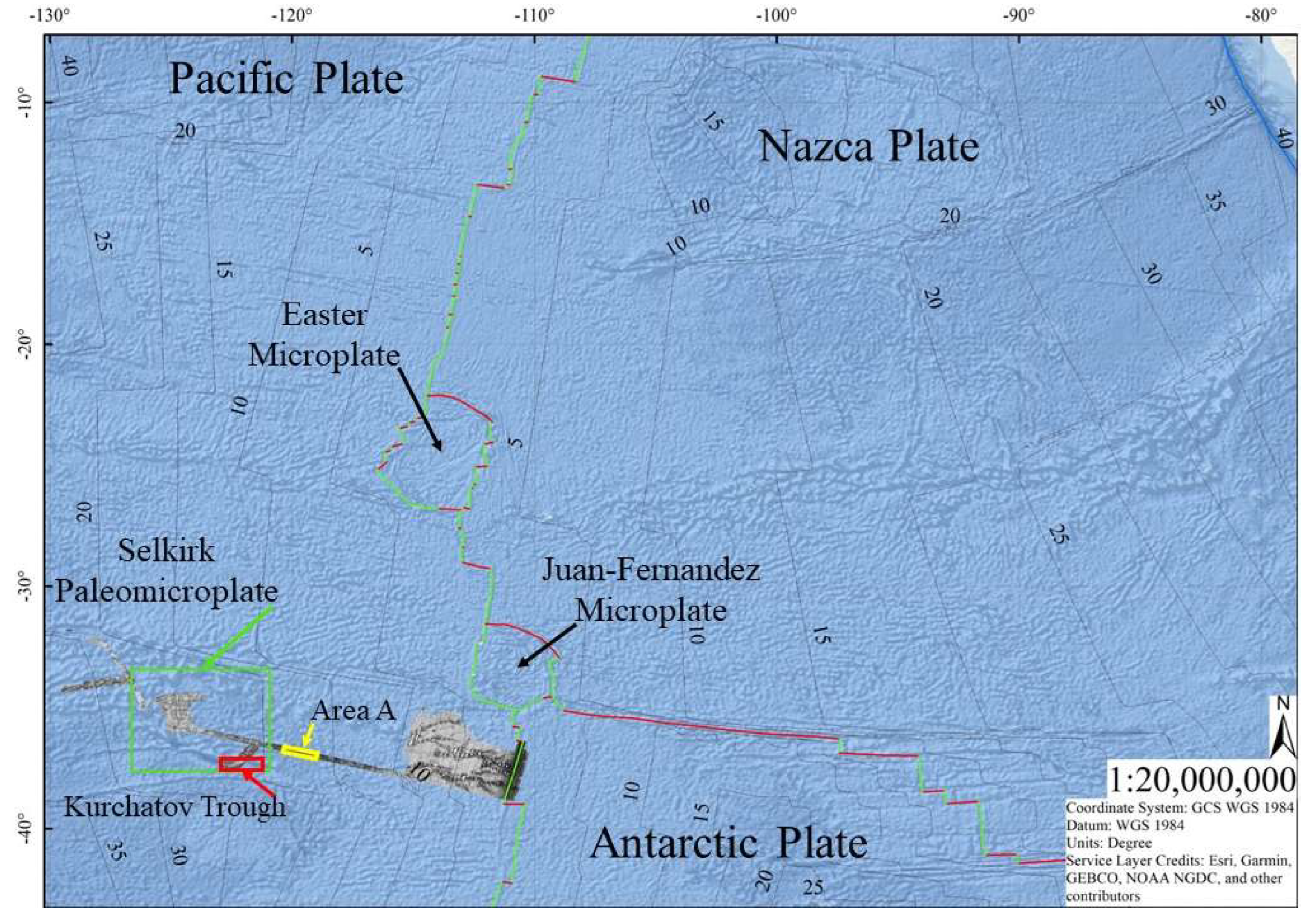
Figure 2.
Stack line comparisons of the three surfaces showing zonal statistics for median and standard deviation based on 60 zones of 90 x 90 km. The MB-SystemTM surface for backscatter in dB is shown in blue, the MB-SystemTM surface for backscatter in 8-bit is shown in grey, and the scanned paper plot of backscatter digitized in 8-bit is shown in orange. Top panel shows zonal statistics for standard deviation as an indicator of zonal homogeneity. Bottom panel shows zonal statistics for median backscatter values; note median backscatter values for ‘MEDIAN_BS’ surface have been normalized from dB value to 8-bit values for comparison with 8-bit surfaces. The stack line trends show all three surfaces share similar zonal statistics at this resolution, indicating all three surfaces may work comparably for analyses.
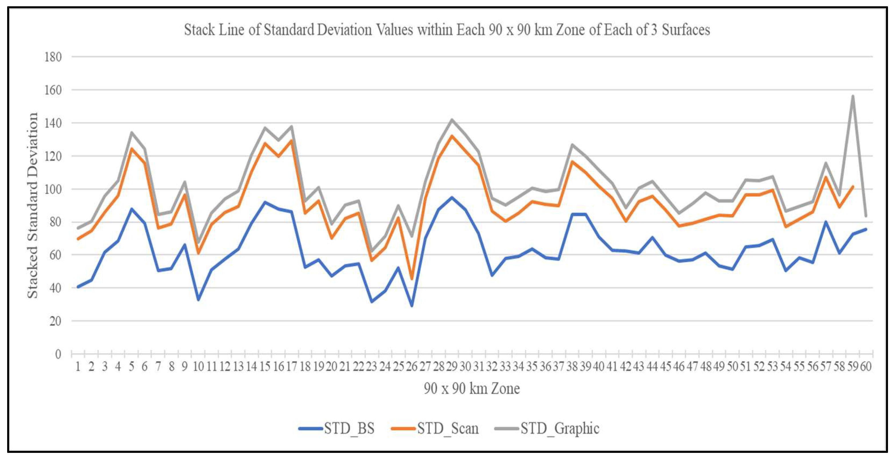
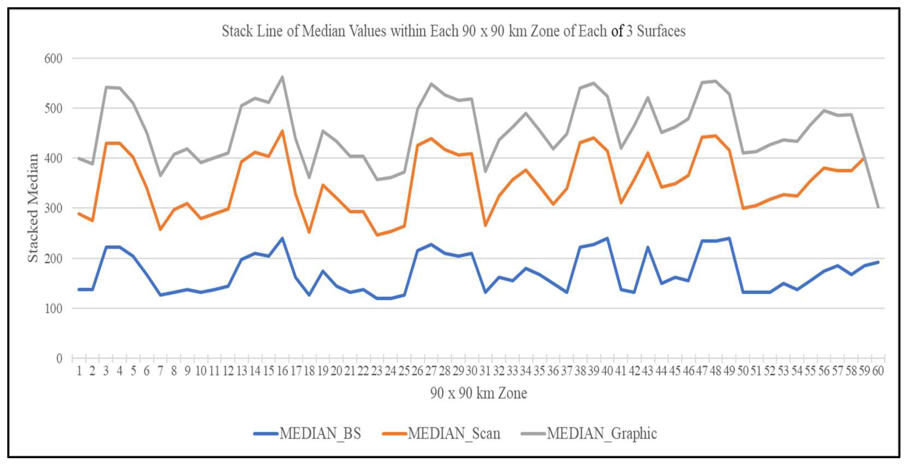
Figure 3.
Backscatter data grouped into zones of 1° of longitude, labeled by number at top of figure.
Figure 3.
Backscatter data grouped into zones of 1° of longitude, labeled by number at top of figure.
Figure 4.
Stack line of all 3 surfaces showing the percentage of the total high backscatter and low σ cells, from respective surfaces, present in each 1° longitudinal zone. ‘BS’ (blue line) refers to the dB intensity chart generated in MB-SystemTM; ‘Scan’ (green line) refers to digitized and georeferenced 8-bit graphic paper chart; ‘Graph’ (grey line) refers to the 8-bit backscatter chart generated in MB-SystemTM. .
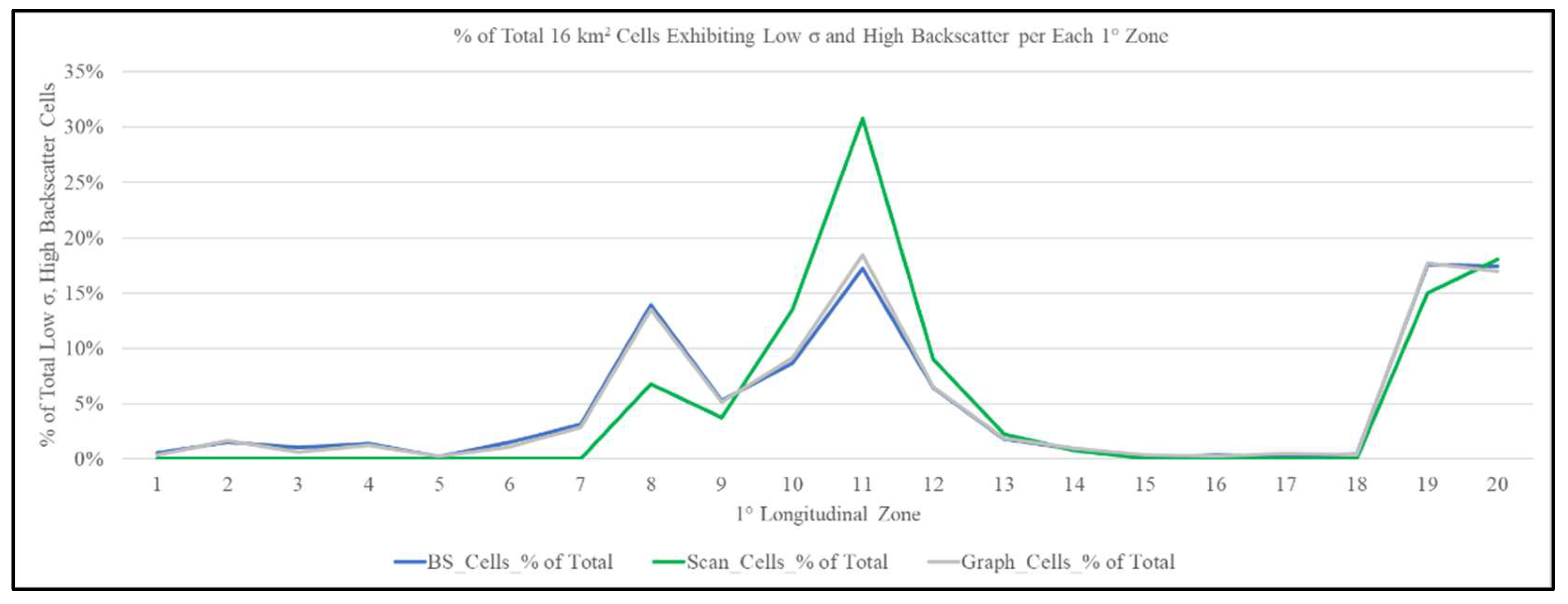
Figure 5.
Zonal analysis output for 4 km X 4 km filtered to areas with low σ and high backscatter value. These zones are shown in purple. Small fractional areas exist within the data, with three apparent clusters labeled in figure.
Figure 5.
Zonal analysis output for 4 km X 4 km filtered to areas with low σ and high backscatter value. These zones are shown in purple. Small fractional areas exist within the data, with three apparent clusters labeled in figure.
Figure 6.
Stack line of all 3 surfaces showing the percentage of the total high backscatter and low σ cells, from respective surfaces, present in each 1° longitudinal zone as filtered to areas of low slope, water depths below the local CCD, low sedimentation rate, and seafloor >2 Ma. ‘BS’ (blue line) refers to the dB intensity chart generated in MB-SystemTM; ‘Graph’ (green line) refers to the 8-bit backscatter chart generated in MB-SystemTM; ‘Scan’ (grey line) refers to digitized and georeferenced 8-bit graphic paper chart. .
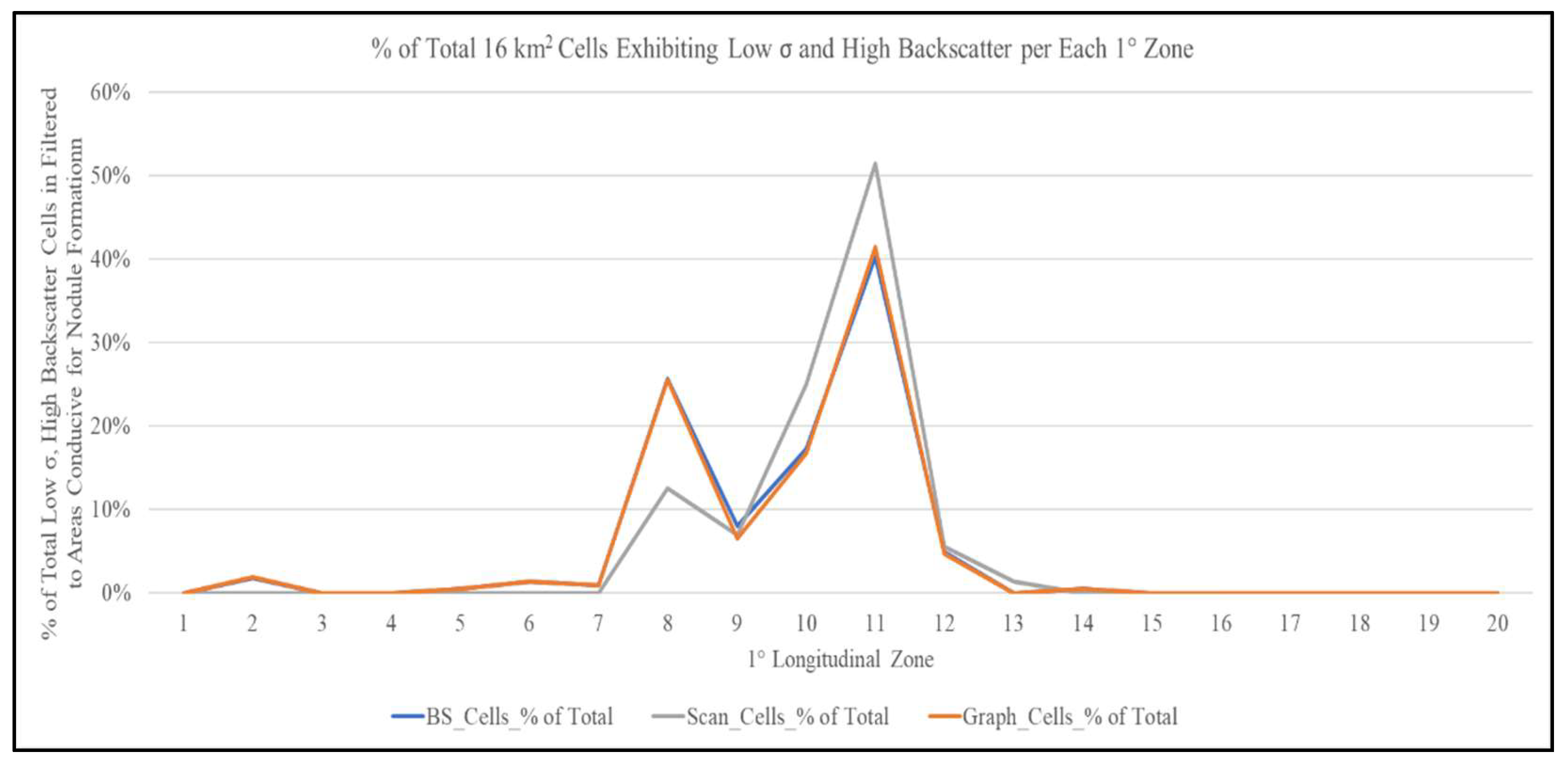
Figure 7.
Zonal analysis output for 4 km X 4 km filtered to areas with low backscatter σ and high backscatter value, and constrained to areas conducive for nodule presence in terms of slope, water depth, sedimentation rate, and seafloor age. Zones likely to contain nodules are shown in purple. Small fractional areas exist within the data, with two apparent clusters labeled in figure.
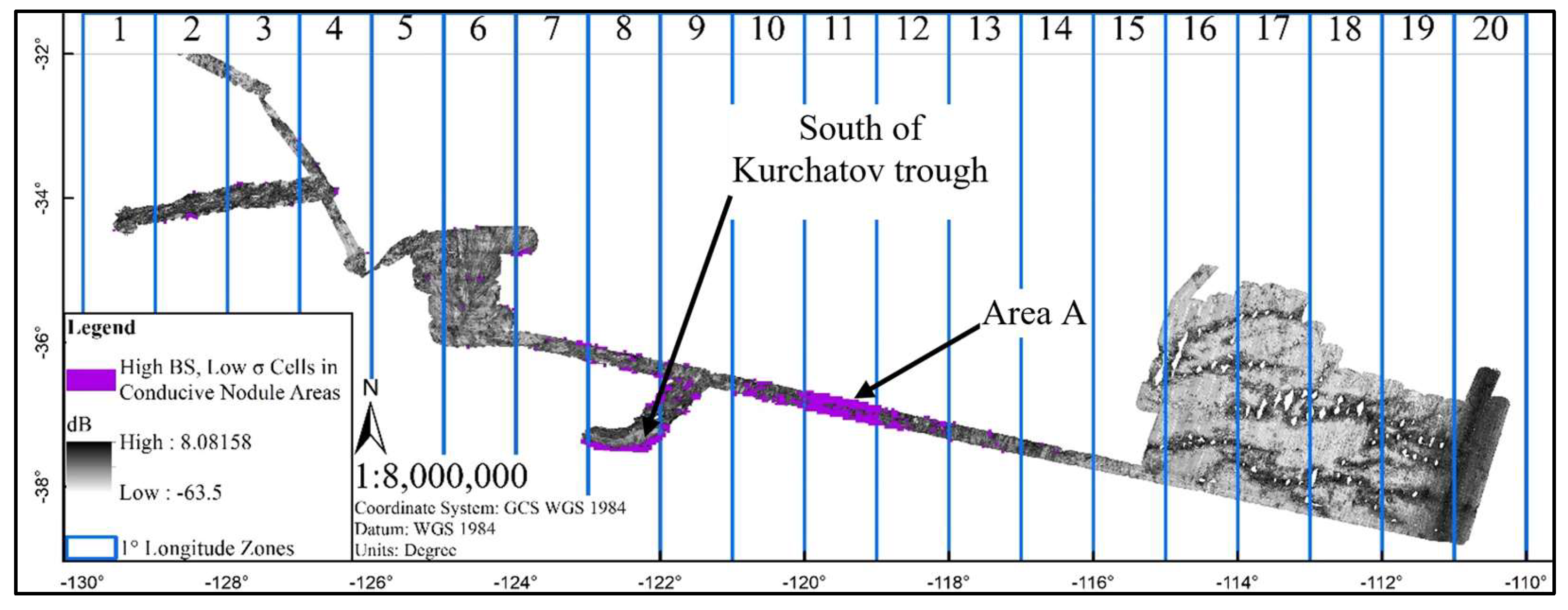
Figure 8.
Sites within the backscatter data where across-track angular response diagrams were generated based on backscatter raster values. Sites are ordered 1 to 10, labeled in figure and outlined in red, from youngest near EPR to oldest in the furthest northwest extent of the data. Table 3 describes each location.
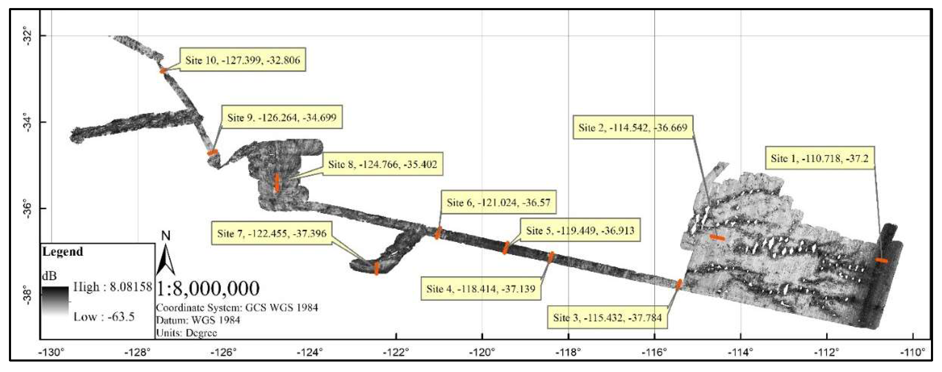
Figure 9.
Angular response diagrams from backscatter value surface in terms of dB. Site descriptions correspond to descriptions in Table 3. Site 5, corresponding to Area A, exhibits the flattest line and highest mean backscatter. Site 1, corresponding to the EPR, exhibits similar backscatter but higher variability. Site 7, corresponding to the Kurchatov trough, shows greater variability, though the 40 – 60° range aligns with the diagrams of Sites 1 and 5.
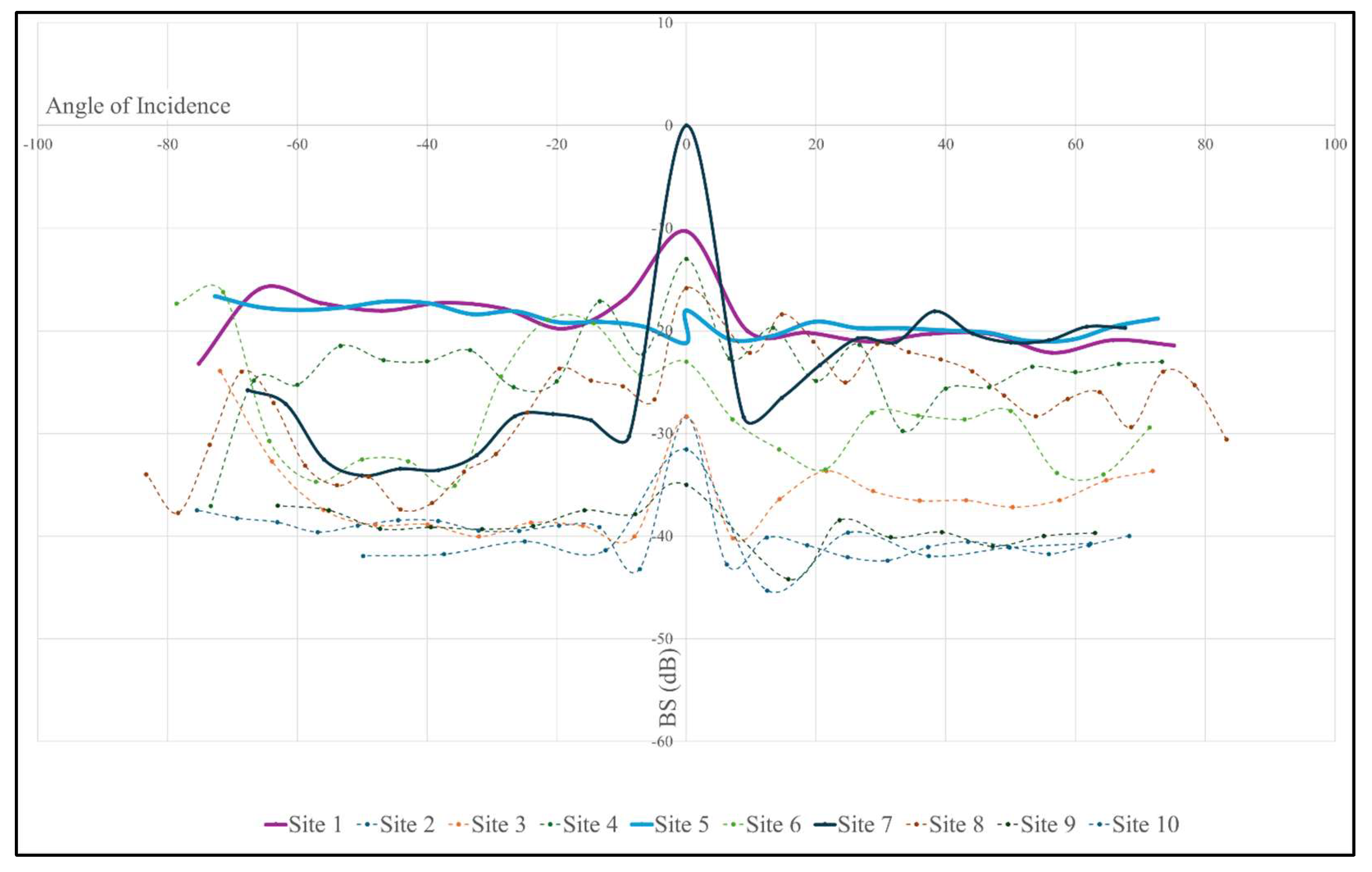
Figure 10.
Angular response diagrams from backscatter value surface in terms of dB. Site descriptions correspond to descriptions in Table 3. Model profiles for several substrate types in terms of 15 kHz angular response as described in the handbook [98] are shown.
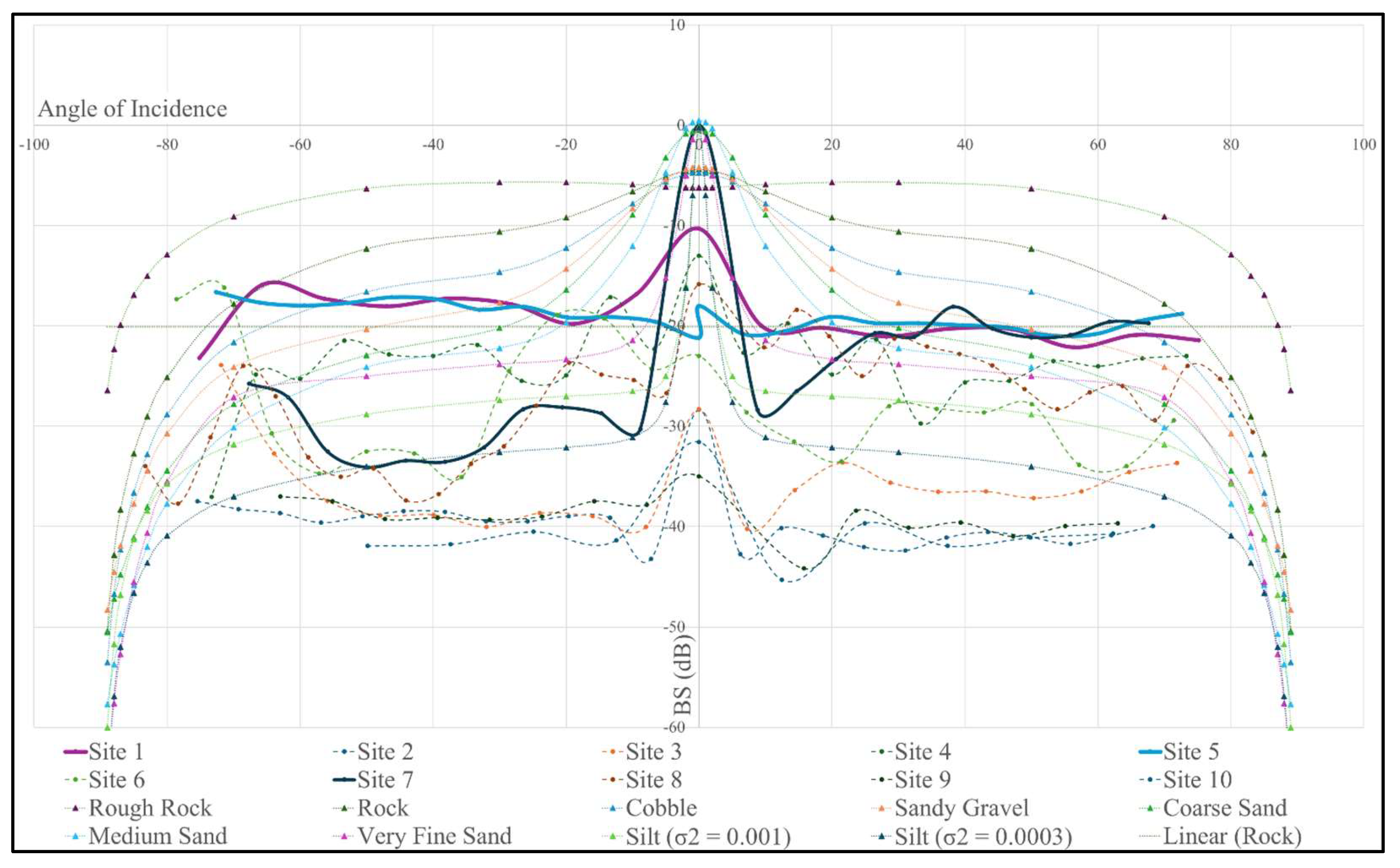
Figure 11.
Angular response diagrams from backscatter value surface in terms of dB. Site descriptions correspond to Table 3. Model profiles for several substrate types in terms of 15 kHz angular response as described in the handbook [98] are shown. Model profiles for several substrate types, including nodules at two abundance levels, in terms of 12 kHz angular response from a study site in the western Pacific Ocean are labeled in the graph (adapted from Yang et al. (2020)) [46]. Note relatively high, uniform backscatter values for the 40 kg/m2 nodule profile; note relatively high, uniform backscatter values for Site 5 (Area A). This qualitative comparison of angular response diagrams suggests abundance nodules exist in Area A.
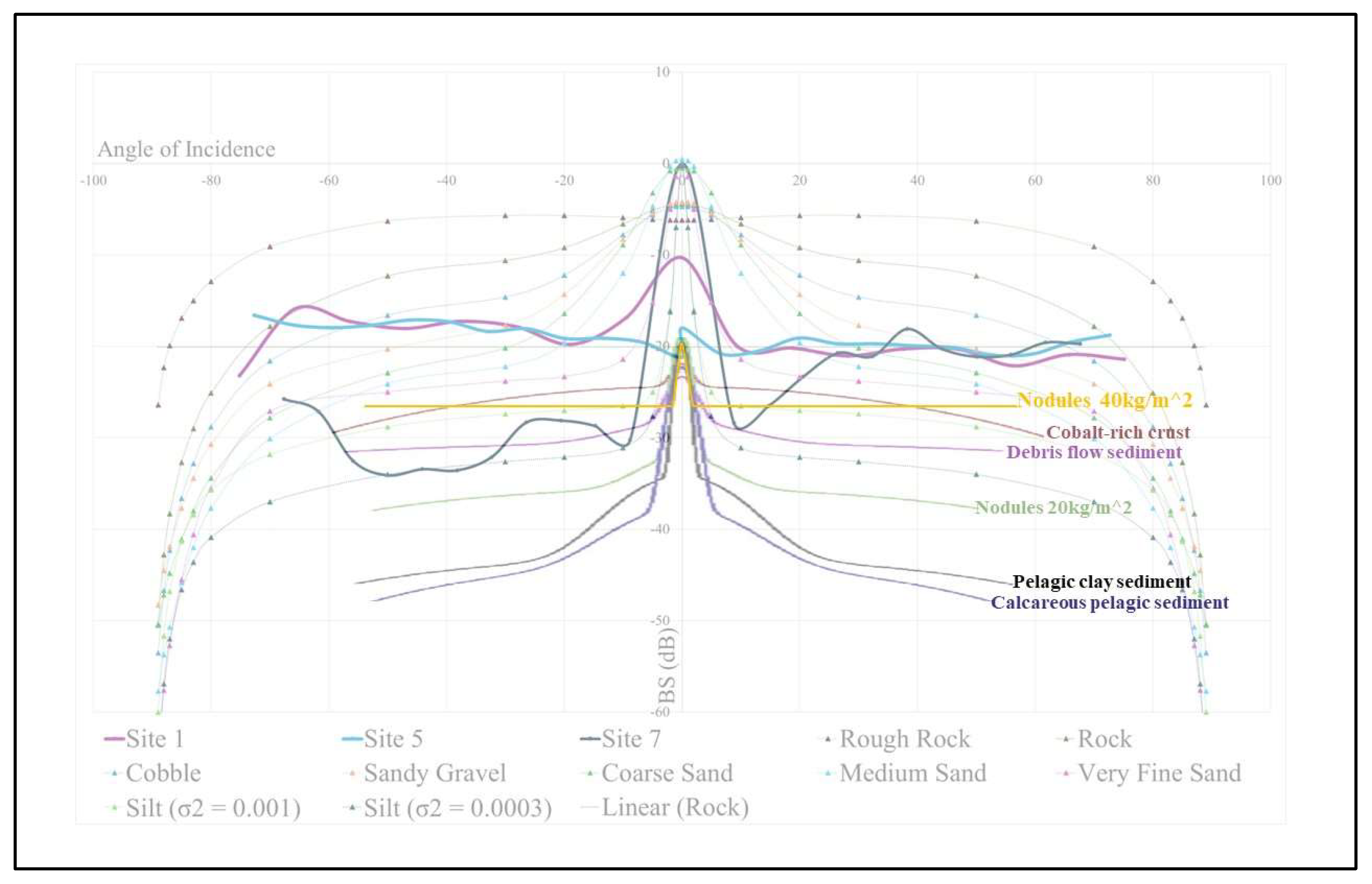

Table 1.
Distribution of high backscatter and low σ cells by 1° longitudinal zones for each of three respective surfaces. ‘BS’ refers to the dB intensity chart generated in MB-SystemTM; ‘Scan’ refers to digitized and georeferenced 8-bit graphic paper chart; ‘Graph’ refers to the 8-bit backscatter chart generated in MB-SystemTM. .
| 1° Longitude Zone | BS_Cells_% of Total | Scan_Cells_% of Total | Graph_Cells_% of Total |
|---|---|---|---|
| 1 | 0.59% | 0.00% | 0.38% |
| 2 | 1.52% | 0.00% | 1.63% |
| 3 | 1.06% | 0.00% | 0.63% |
| 4 | 1.41% | 0.00% | 1.25% |
| 5 | 0.23% | 0.00% | 0.25% |
| 6 | 1.52% | 0.00% | 1.13% |
| 7 | 3.17% | 0.00% | 2.89% |
| 8 | 13.95% | 6.77% | 13.55% |
| 9 | 5.28% | 3.76% | 5.14% |
| 10 | 8.68% | 13.53% | 9.16% |
| 11 | 17.23% | 30.83% | 18.44% |
| 12 | 6.45% | 9.02% | 6.52% |
| 13 | 1.76% | 2.26% | 1.88% |
| 14 | 0.94% | 0.75% | 1.00% |
| 15 | 0.12% | 0.00% | 0.38% |
| 16 | 0.35% | 0.00% | 0.25% |
| 17 | 0.23% | 0.00% | 0.50% |
| 18 | 0.47% | 0.00% | 0.38% |
| 19 | 17.58% | 15.04% | 17.69% |
| 20 | 17.47% | 18.05% | 16.94% |
Table 2.
Distribution of high backscatter value and low backscatter σ cells by 1° longitudinal zones for each of three surfaces, constrained to areas conducive for nodule presence in terms of sedimentation rate, water depth, seafloor slope, and seafloor age. Grey-shaded table rows indicate 1° longitudinal zones containing no cells exhibiting both high backscatter value and low backscatter σ after such applying such constraints. ‘Scan’ refers to digitized and georeferenced 8-bit graphic paper chart; ‘Graph’ refers to the 8-bit backscatter chart generated in MB-SystemTM; ‘BS’ refers to the dB intensity chart generated in MB-SystemTM.
| 1° Longitude Zone | BS_Cells_% of Total | Scan_Cells_% of Total | Graph_Cells_% of Total |
|---|---|---|---|
| 1 | 0.00% | 0.00% | 0.00% |
| 2 | 1.77% | 0.00% | 1.86% |
| 3 | 0.00% | 0.00% | 0.00% |
| 4 | 0.00% | 0.00% | 0.00% |
| 5 | 0.44% | 0.00% | 0.47% |
| 6 | 1.33% | 0.00% | 1.40% |
| 7 | 0.88% | 0.00% | 0.93% |
| 8 | 25.66% | 12.50% | 25.58% |
| 9 | 7.96% | 6.94% | 6.51% |
| 10 | 17.26% | 25.00% | 16.74% |
| 11 | 40.27% | 51.39% | 41.40% |
| 12 | 4.87% | 5.56% | 4.65% |
| 13 | 0.00% | 1.39% | 0.00% |
| 14 | 0.44% | 0.00% | 0.47% |
| 15 | 0.00% | 0.00% | 0.00% |
| 16 | 0.00% | 0.00% | 0.00% |
| 17 | 0.00% | 0.00% | 0.00% |
| 18 | 0.00% | 0.00% | 0.00% |
| 19 | 0.00% | 0.00% | 0.00% |
| 20 | 0.00% | 0.00% | 0.00% |
Table 3.
Angular response diagram statistics for 10 test sites from the data. Column ‘Absolute Average Difference between Trendline Intercept and BS at Incidence Angles’ indicates the general flatness of the profile. .
Table 3.
Angular response diagram statistics for 10 test sites from the data. Column ‘Absolute Average Difference between Trendline Intercept and BS at Incidence Angles’ indicates the general flatness of the profile. .
| Site | Area Name | Mean BS (dB) | Absolute Difference between Trendline Intercept and Nadir | Absolute Average Difference between Trendline Intercept and BS at Incidence Angles |
|---|---|---|---|---|
| 1 | EPR | -19.69 | 8.687355 | 2.29 |
| 2 | Survey flat area between volcanic features west of EPR | -40.22 | 11.8692 | 1.75 |
| 3 | Transit southeast of / younger than Area A | -36.53 | 7.593326 | 2.91 |
| 4 | Transit slightly southeast of / younger than Area A | -23.49 | 10.575 | 2.73 |
| 5 | Area A | -19.283 | 1.283 | 1.10 |
| 6 | Transit slightly NW of Area A | -28.5 | 4.996 | 4.65 |
| 7 | Kurchatov trough | -26.14 | 24.942 | 5.62 |
| 8 | Selkirk structure | -27.72 | 10.829983 | 3.29 |
| 9 | Transit north of Selkirk structure, apparent low BS | -39.42 | 4.057381 | 1.37 |
| 10 | Transit in NW data area, apparent low BS | -42.05 | 9.019949 | 2.00 |
Disclaimer/Publisher’s Note: The statements, opinions and data contained in all publications are solely those of the individual author(s) and contributor(s) and not of MDPI and/or the editor(s). MDPI and/or the editor(s) disclaim responsibility for any injury to people or property resulting from any ideas, methods, instructions or products referred to in the content. |
© 2024 by the authors. Licensee MDPI, Basel, Switzerland. This article is an open access article distributed under the terms and conditions of the Creative Commons Attribution (CC BY) license (http://creativecommons.org/licenses/by/4.0/).
Copyright: This open access article is published under a Creative Commons CC BY 4.0 license, which permit the free download, distribution, and reuse, provided that the author and preprint are cited in any reuse.


