Submitted:
21 October 2024
Posted:
22 October 2024
You are already at the latest version
Abstract
US life expectancy now lags significantly behind the majority of high-income countries, having grown more slowly since 1980 for reasons that are not evident and have been debated. An exploratory system dynamics model is presented that reproduces the full pattern of US life expectancy from 1960 to the present. Multiple socioeconomic and behavioral factors help to explain the historical pattern, two of them apparently most responsible for the stagnation since 1980: the growth of obesity and the leveling off of growth in social spending. Some of the factors in the model are traced back to earlier causes, and obesity’s growth in particular is traced back to excess growth in private health care spending and its adverse effect on workers’ wages. The model’s base run does a good job of reproducing a variety of historical time series data going back to the 1960s, and counterfactual testing produces plausible results. The model may thus be considered a reasonable starting point for more conclusive future modeling of US life expectancy.
Keywords:
life expectancy
; causes of death
; obesity
; health care spending
; economic inequality
; social spending
; simulation
; system dynamics
; counterfactual testing
; social trust
1. Introduction
Life expectancy at birth (LEB) in the United States grew robustly from 1960 to 1980, in parallel with other high-income countries; but that growth slowed after 1980, and US LEB was essentially flat after 2010, even before the advent of COVID-19. By 2022, it was 77.5 years, far below the 83-plus years of eight OECD countries (led by Japan at 84.5) and three years below the OECD average [1].
Many factors have been posited for the stagnation of US LEB, some studies focusing on growth or flattening in the rates of specific causes of premature death (including diabetes, heart disease, drug overdoses, suicides, and vehicle crashes) [2,3,4,5,6], while others have looked at economic and social determinants and the roles of health and social spending [7,8,9,10,11,12,13,14].
A recent multivariate statistical analysis found several factors beyond GDP per capita (obesity, education, social spending, alcohol consumption, and opioid prescriptions), that together accounted for a large portion of the LEB differentials among 34 OECD countries. But these factors explained only half of the US underperformance relative to what would be expected based on GDP per capita alone [15].
Thus, it makes sense to focus on the US as a unique case. This paper uses system dynamics simulation to explore a particular social theory in the light of available evidence over a 60-year period and what it may imply for policy. Such dynamic modeling has been used for decades to study many health and social issues [16,17,18,19,20,21], but not the long-term dynamics of US LEB.
What makes the US uniquely vulnerable? Two frequently mentioned possibilities are its highest-in-the-world rates of obesity [22] and health care spending [14,23]. Higher health care spending correlates with better outcomes in other OECD countries, but not in the US [15]. The US is the one country where most of the under-65 population is covered by private health insurance plans rather than by the government. With the growth in health care spending, these plans have become increasingly expensive since the 1980s, driving down take-home pay for many workers or exposing them to the possibility of medical bankruptcy [24].
But why would stagnant wages for some workers have society-wide effects, when many other Americans have experienced income growth? Indeed, GDP per capita, a primary driver of LEB [9,15,25], has grown robustly in the US for many decades. The argument must be about the corrosive effects of unequal income; about what happens when some workers see their take-home pay stagnating while others are doing much better. Putnam and Garrett document in detail the adverse social, cultural, and political consequences that have accompanied increasing income inequality in the US since the 1970s. These include a decline in social solidarity, social trust, and labor unions, and an increase in corporate power and deaths of despair [26]. Income inequality, in turn, may have laid the groundwork for the obesity epidemic [22].
On the surface, then, a plausible case can be made for the idea that growing private health care costs have been the primary culprit behind the stagnation of US LEB. This paper seeks to determine whether this social theory (along with other important factors like education and social spending) can reproduce the historical evidence when it is put in the testable form of a simulation model. Also, counterfactual tests of the model are done to reveal the relative significance of key causal factors.
2. Materials and Methods
2.1. Data
The modeling process started with a scan of the relevant literature and of well-established, long-standing data sources. The prior analysis of OECD LEB differentials also helped in identifying potential factors [15].
Table 1 is a list of variables that were found useful, statistically and when simulated, for explaining the historical trajectory of US LEB. In all cases, the data were reported from 1960 (or the early 1960s) through the 2020s or late 2010s; in most cases, the frequency of reporting was annual or biannual. (Appendix 1 in Supplementary File S1 provides a full table of time series data values, including UNDP medium-variant population projections through 2040.)
Other data variables were evaluated but not found useful for helping to explain the historical US LEB pattern. Poverty and disability, for example, both declined overall from 1980 to 2018, with some fluctuation but no evidence of stagnation [27,28,29].
Additionally, annual death rates by 5-year age group and major cause (non-communicable disease, communicable and other disease, and injury) [30] were examined closely and tested with an algebraic LEB calculator to see whether certain age-specific trends, such as a growing rate of deaths from injury among the elderly since 1990 [31], might have had a significant adverse effect on life expectancy. No such significant effect was found. (See Appendix 2 in Supplementary File S1.)
2.2. Causal-Loop Diagram (Model Overview)
Figure 1 presents a causal-loop diagram overview of the resulting system dynamics model. The diagram shows eight factors directly affecting LEB, as follows:
1) GDP per capita (GDPPC): GDPPC was the most important differentiating factor in the OECD LEB analysis [15]. It is modeled here as the accumulation of an exogenous growth rate that gives the correct GDPPC trajectory through 2021 and is assumed to continue after that at 1% per year, the approximate historical average.
2) Obese fraction of age 18-plus: Obesity was a second differentiator in the OECD LEB analysis [15]. It is modeled here as a stock variable driven upward by declines in the wage/salary fraction of GDP (as an indicator of income inequality), as well as by self-reinforcing social influence. The effect of obesity on LEB is modeled in part with a lengthy delay, reflecting the gradual progression of chronic diseases related to obesity.
3) College graduate fraction of age 25-plus: College education was a third differentiator in the OECD LEB analysis [15]. It is modeled here with population aging chains including births, net immigration, and deaths, and age groups 0-24, 25-64, and 65-plus. This structure was tuned to produce correct trajectories for total population by age group, high school graduates, and college graduates. The model includes inflows of adults getting high school and college degrees after age 25; these inflows are necessary to produce a good fit to the 25-plus data. The high school graduation rate by age 18 is modeled exogenously, rising from 70% in 1960 to 88% by 2020. The college graduation rate by age 25 is modeled algebraically, starting with high school graduates and adding a strong positive influence from government social spending, causing this graduation rate to rise from 10% in 1960 to 37% in 2010-2017.
4) Government social spending fraction of GDP: Social spending was a fourth differentiator in the OECD LEB analysis [15]. It is modeled here exogenously using the data series described in Table 1 (source: OECD) and is a potentially key policy input.
5) Current smoker fraction of age 18-plus: Smoking did not emerge from the OECD LEB analysis as a differentiating factor, likely due to confounding cross-effects [15]. Nonetheless, smoking is undeniably a major mortality risk affecting LEB [2,3,32]. It is modeled as a stock variable driven downward by the increasing college graduate fraction as well as by self-reinforcing social influence. The effect of smoking on LEB is modeled in part with a lengthy delay, reflecting the gradual progression of chronic diseases related to smoking.
6) Suicide rate: This variable was not available across countries for the OECD LEB analysis, but it has been described as a key factor affecting US LEB, having grown significantly since its lowest point in 2000 [3,4,5]. It is modeled algebraically, tending to fall with increases in the high school graduate fraction of adults and increases in social spending and tending to rise with declines in social trust. (See Putnam/Garrett on deaths of despair, p. 43 [26].)
7) Personal health care spending fraction of GDP: This variable did not emerge from the OECD LEB analysis as a differentiating factor, and the evidence is mixed for a positive net effect of additional health care spending on US LEB [13,14]. Nonetheless, quality health care undeniably saves many lives and is often resource intensive, so a small positive influence of health care spending on LEB is assumed in the model. But the model also includes the adverse effect that growing health care spending has had on take-home pay in the US, as described above. This variable is modeled exogenously using the data series described in Table 1 (source: NHE) and can be altered in counterfactual testing.
8) COVID-19: The model uses a default input time series to represent the spike downward in US LEB that is evident in the data from both UNDP (2020-2021) and CDC (2020-2023); see Table 1. Recovery of LEB from the multiple adverse health system effects of COVID is assumed to be complete by the end of 2024. The model also includes a link from social trust to the magnitude of the COVID effect on LEB (for counterfactual testing), in line with research suggesting that greater social trust can improve the public health response [33].
All variables in this diagram are supported by historical data (see Table 1); COVID-19 effect on LEB is inferred from the downward spike of LEB reported by UNDP for 2020-2021 and CDC for 2020-2023.
Social trust was mentioned above in connection with its effects on suicide and the impact of COVID. Social trust declined from about 60% in the early 1960s to 37% in the early 1990s, then temporarily recovered during the late 1990s and early 2000s to a peak of 46%, then declined further to 33% by 2014. It is modeled here in line with the analysis of Putnam/Garrett, which describes a syndrome of reduced social, political, and economic solidarity since the 1960s [26]. The dynamic hypothesis here is that growing income inequality (operationalized as a decline in wages and salaries as a fraction of GDP) led to reduced social solidarity (and the related concept of social trust), which, in turn, undermined union membership, which further exacerbated the relative decline in wages/salaries.
The entry point for this vicious cycle in the model is the growth of private health care spending, which, as noted above, has been a major reason for stagnating take-home pay for wage workers. In the model, monotonic growth in health care spending from 1960 to 2020 leads to monotonic adverse trajectories for the wage/salary fraction, social solidarity, and unionization.
An inverted-U-shaped exogenous time series is introduced during 1996-2005 to recreate the temporary resurgence of social trust seen during those years; that temporary resurgence has been noted by others but not explained [34]. It is the only difference between social solidarity and social trust in the model, and it is included because it may help explain some of the down-and-up pattern (with its lowest point in 2000) seen in the US suicide rate as a response to changes in social trust.
2.3. Establishing a Base Run
The simulation model (built with the VensimTM software package) has 192 elements, of which 28 are uncertain parameters (mostly relational exponents and coefficients) related to the structure shown in Figure 1. (A full model listing is presented as Appendix 3 in Supplementary File S1.)
Because of the model’s relatively parsimonious structure, most of its uncertain parameters could be adjusted to achieve a good fit to the data without ambiguity. However, this was less straightforward in the case of 7 exponents corresponding to the 7 primary factors affecting LEB described above (i.e., all with the exception of COVID-19).
The estimation challenge was largely due to collinearity among the explanatory factors. Six of the 7 primary factors, all except the suicide rate, moved monotonically upward or downward during the historical period, though with somewhat different patterns of acceleration and deceleration. Prior information suggested only that the positive effect of health care spending on LEB is likely weak [12]. Establishing reasonable values for the other exponents thus required some experimentation, starting with a neutral assumption of equal exponents for the factors other than health care spending, and then adjusting to achieve a better fit to the roughly S-shaped LEB pattern. This was tentatively established as the base run, though with some remaining uncertainty around the LEB exponents..
3. Results
3.1. Base Run Results
Figure 2. presents selected graphical results from the base run and comparison with historical data. Table 2 presents quantitative summaries for 12 historical time series and model goodness of fit. The MAPE (mean absolute percentage error) and MAEM (mean).
The model’s LEB grows from its initial value of 69.8 years to 77.4 years in 2020; the latter is identical to the value reported by UNDP. In the base run, this increase of 7.6 years is attributable to changes in the 8 LEB factors as follows: due to GDPPC growth +2.5 years; due to obesity growth -2.4 years; due to college graduate growth +3.8 years; due to social spending growth +3.4 years; due to smoking decline +1.8 years; due to suicide rate (slight net decline from 1960 to 2020) +0.1 years; due to health care spending growth +0.5 years; and due to COVID -2.1 years.
3.2. Counterfactual Testing
Counterfactual tests were performed to clarify the roles of two key exogenous model drivers: health care spending and social spending. In the first test (CF1), the personal health care spending fraction of GDP is held constant after 2000 at 11.3% rather than rising to 14.5% by 2010 and 15.2% by 2021. See the left-side graph of Figure 3. This test asks, in essence, to what extent LEB was adversely affected by the consequent decline of social trust, via rising obesity and suicide (see Figure 1), after 2000.
In the second test (CF2), the government social spending fraction of GDP steps up from its 2000 value of 14.1% to 24% in 2001 and beyond, rather than its more gradual historical rise to 19% in 2010 and 18.2% in 2019 (followed by 23.9% in 2020, 22.7% in 2021, and assumed 20% by 2024 and beyond). See the right-side graph of Figure 3. This test asks, in essence, to what extent the stagnation of US LEB in the 2000s could have been avoided by greater social spending, which boosts LEB directly (e.g., by mitigating the health risks of poverty), and through greater college education and reduced smoking and suicide (see Figure 1).
A third counterfactual test (CF3) combines the assumptions of the first two tests, allowing one to see whether their impacts on LEB are simply additive or rather overlapping (less than additive) or synergistic (more than additive).
Selected output variables from the base run and the three counterfactuals are graphed in Figure 4.
The CF1 test (flattened health care spending) causes the wages/salaries fraction to flatten at 0.45 after 2000 rather than declining to 0.435 by 2025 as it does in the base run. This has beneficial effects for obesity, which flattens at 30% soon after 2000 rather than rising to 40% by 2025 as it does in the base run. The flattening of wages/salaries in CF1 also causes social trust to flatten at 0.38 after 2000 rather than declining to 0.335 by 2025. This reduces suicide by about 5%. The beneficial impact of reduced obesity in CF1 is to improve LEB by 0.52 years in 2025 and by 0.71 years in 2040; the suicide improvement contributes only negligibly.
4. Discussion
The system dynamics model described here was built to test whether a relatively parsimonious theory of US life expectancy dynamics could produce patterns over 60 years that are a good fit to historical data and give plausible results when tested counterfactually. The model seems to clear this bar, and it may thus be considered a reasonable starting point for further modeling work on US LEB.
However, the model leaves some uncertainties unresolved, both in terms of its calibration and parts of the theory itself. With regard to calibration, uncertainty remains about the strength of the several factors directly affecting LEB. The current settings suggest that, over the past 60 years, US LEB has benefited most from the growth of college education, social spending (esp. 1970-1980), and GDP per capita, plus the decline of smoking; and has been hindered most (prior to COVID-19) by the growth of obesity since the late 1970s and stagnation in social spending during the 2010s. It is possible that a more careful look at the existing literature on the mortality risks of smoking [32,35] and obesity [36,37] may help refine these estimates.
With regard to the theory, the greatest uncertainty is about the causal chain from higher health care spending to lower wages and then to the growth of obesity. The model’s fit to history is excellent along this chain, but one may think of other important factors that are part of the full story. First, the problem of income inequality and stagnant worker’s wages has arisen not only in the US but also in many other countries, and the drivers outside the US are not health care costs but rather the spread of digital technologies, automation, and globalization [38].
Second, the growth of obesity in the US is often explained as a consequence of the reduced price of sweeteners and the rapidly growing popularity of fast-food restaurants starting in the 1970s [22]. Perhaps stagnating wages did in fact lay the groundwork for the popularity of fast food, but proving this point would require more investigation.
Note also that the model here includes only a high-level portrayal (through the use of delay functions) of the onset and progression of chronic diseases associated with obesity and smoking; and does not show how their mortality risks increase with age. Previous system dynamics models have addressed these topics [39,40], so adding such detail is certainly possible, though it might expand the size of the model significantly.
In 2011, the National Research Council indicated that a systems framework was needed for gaining a deeper understanding of US life expectancy, one that could guide national policy [2]. The model presented here is a first step in that direction and could be improved with more detail and evidence.
Supplementary Materials
Supplementary file S1 contains Appendices 1, 2, and 3.
Funding
This research received no external funding.
Data Availability Statement
Publicly available data were analyzed in this study; see Appendices 1 and 2. The simulation model’s equations and parameters are listed in Appendix 3.
Conflicts of Interest
The author declares no conflict of interest.
References
- OECD. 2024. Indicators: Life expectancy at birth. OECD data portal. Available from: https://data.oecd.org.
- National Research Council (US). 2011. Explaining divergent levels of longevity in high-income countries. Crimmins EM, Preston SH, Cohen B (Eds.) Washington DC: National Academies Press, 194 pp.
- Woolf SH, Schoonmaker H. 2019. Life expectancy and mortality rates in the United States, 1959-2017. JAMA 322(20):1996-2016. [CrossRef]
- Roser M. 2020. Why is life expectancy in the US lower than in other rich countries? Our World in Data (online). Available from: https://ourworldindata.org/us-life-expectancy-low.
- Harper S, Riddell CA, King NB. 2021. Declining life expectancy in the United States: missing the trees for the forest. Annual Rev Pub Health 42:381-403. [CrossRef]
- Muennig P, Fiscella K, Tancredi D, Franks P. 2010. The relative health burden of selected social and behavioral risk factors in the United States: implications for policy. Am J Pub Health 100:1758-1764.
- Braveman PA, Cubbin C, Egerter S, Williams DR, Pamuk E. 2010. Socioeconomic disparities in health in the United States: what the patterns tell us. Am J Pub Health 100(S1):S186-S196. [CrossRef]
- Woolf SH, Braveman P. 2011. Where health disparities begin: the role of social and economic determinants-and why current policies may make matters worse. Health Aff (Millwood) 30(10):1852-1859. [CrossRef]
- Chetty R, Stepner M, Abraham S, Lin S, Scuderi B, Turner N, et al. 2016. The association between income and life expectancy in the United States, 2001-2014. JAMA 315(16):1750-1766. [CrossRef]
- Bundy JD, Mills KT, He H, LaVeist TA, Ferdinand KC, Chen J, et al. 2023. Social determinants of health and premature death among adults in the USA from 1999 to 2018: a national cohort study. Lancet Pub Health 8:e422-e431. [CrossRef]
- Bradley EH, Elkins BR, Herrin J, Elbel B. 2011. Health and social services expenditures: associations with health outcomes. BMJ Quality & Safety 20:826-831. [CrossRef]
- Rothberg MB, Cohen J, Lindenauer P, Maselli J, Auerbach A. 2010. Little evidence of correlation between growth in health care spending and reduced mortality. Health Aff (Millwood) 29:1523-1531. [CrossRef]
- Weaver MR, Joffe J, Ciarametaro M, Dubois RW, Dunn A, Singh A, et al. 2022. Health care spending effectiveness: estimates suggest that spending improved US health from 1996 to 2016. Health Aff (Millwood) 41(7):994-1004. [CrossRef]
- Kindig D, Chowkwanyun M. 2020. Why did cross-national divergences in life expectancy and health care expenditures both appear in the 1980s? Am J Pub Health 110(12):1741-1742. [CrossRef]
- Homer JB. 2023. Life expectancy in the U.S. and other OECD countries: a multivariate analysis of economic, social, and behavioral factors. June 2024. Available from: https://www.academia.edu/121497712/Life_Expectancy_in_the_U_S_and_Other_OECD_Countries_A_Multivariate_Analysis_of_Economic_Social_and_Behavioral_Factors.
- Sterman JD. 2000. Business Dynamics: : Systems Thinking and Modeling for a Complex World. Boston: McGraw-Hill; p. 874.
- Homer JB. 2012. Models That Matter: Selected Writings on System Dynamics 1985-2010. Barrytown, New York: Grapeseed Press.
- Homer J, Milstein B, Hirsch GB, Fisher ES. 2016. Combined regional investments could substantially enhance health system performance and be financially affordable. Health Aff (Millwood) 35(8):1435-1443. [CrossRef]
- Darabi N, Hosseinichimeh N. 2020. System dynamics modeling in health and medicine: a systematic literature review. Syst Dyn Rev 36(1):29-73. [CrossRef]
- Homer J. 2020. Modeling global loss of life from climate change through 2060. Syst Dyn Rev 36(4):523-535. [CrossRef]
- Homer J, Hirsch GB (eds). 2023. System Dynamics Models for Public Health and Health Care Policy. Basel, Switzerland: MDPI. [CrossRef]
- Temple NJ. 2022. The origins of the obesity epidemic in the USA-lessons for today. Nutrients 14:4253-4260. [CrossRef]
- Altman D. 2024. The two health care cost crises. KFF (online). Available from: https://www.kff.org/from-drew-altman/the-two-health-care-crises.
- Miller BJ, Nyce S. 2023. Healthcare USA: the big paycheck squeeze. WTW Insider 33(5), 8 pp (online). Available from: https://www.wtwco.com/en-us/insights/2023/07/the-big-paycheck-squeeze-the-impacts-of-rising-healthcare-costs.
- Cutler D, Deaton A, Lleras-Muney A. 2006. The determinants of mortality. J Econ Perspectives 20(3):97-120. [CrossRef]
- Putnam RD, Garrett SR. 2020. The Upswing: How America Came Together a Century Ago and How We Can Do It Again. New York: Simon & Schuster.
- US Census Bureau. 2024. Historical poverty tables: people and families, 1959 to 2023. Available from: https://www.census.gov/data/tables/time-series/demo/income-poverty/historical-poverty-people.html.
- Iezzoni LI, Kurtz SG, Rao SR. 2014. Trends in U.S. adult chronic disability rates over time. Disabil Health J. 7(4):402-12. [CrossRef]
- Zajacova A, Margolis R. 2024. Trends in disability and limitations among U.S. adults age 18-44, 2000-2018. Am J Epidemiol. Aug 12:kwae262. [CrossRef]
- Institute for Health Metrics and Evaluation (IHME). 2024. Global health data exchange (GHDx). Available from: https://www.healthdata.org/data-tools-practices/data-sources.
- National Safety Council. 2024. Historical preventable fatality trends; standardized rates. Available from: https://injuryfacts.nsc.org/all-injuries/historical-preventable-fatality-trends/standardized-rate/.
- Jacobs DR, Adachi H, Mulder I, Kromhout D, Menotti A, Nissinen A, et al. 1999. Cigarette smoking and mortality risk: 25-year follow-up of the Seven Countries Study. Arch Intern Med 159:733-740.
- Song E, Yoo HJ. 2020. Impact of social support and social trust on public viral risk response: a COVID-19 survey study. Intl J Envir Res and Pub Health 17:6589-6602. [CrossRef]
- Vallier K. 2020. US social trust has fallen 23 points since 1964. Reconciled (online). Available from: https://www.kevinvallier.com/reconciled/new-finding-us-social-trust-has-fallen-23-points-since-1964/.
- Carter BD, Abnet CC, Feskanich D, Freedman ND, Hartge P, Lewis CE, et al. 2015. Smoking and mortality-beyond established causes. New Engl J Med 372:631-640. [CrossRef]
- Kitahara CM, Flint AJ, de Gonzales AB, Bernstein L, Brotzman M, MacInnis RJ, et al. 2014. Association between Class III obesity (BMI of 40-59 kg/m2) and mortality: a pooled analysis of 20 prospective studies. PLOS Medicine 11(7):e1001673, 14 pp. [CrossRef]
- Prospective Studies Collaboration. 2009. Body-mass index and cause-specific mortality in 900,000 adults: collaborative analyses of 57 prospective studies. Lancet 373:1083-1096. [CrossRef]
- Qureshi Z. 2023. Rising inequality: a major issue of our time. Brookings (online). Available from: https://www.brookings.edu/articles/rising-inequality-a-major-issue-of-our-time.
- Hirsch G, Homer J, Wile K, Trogdon JG, Orenstein D. 2014. Using simulation to compare 4 categories of intervention for reducing cardiovascular disease risks. Am J Public Health 104(7):1187-1195. [CrossRef]
- Clennin M, Homer J, Erkenbeck A, Kelly C. 2022. Evaluating public health efforts to prevent and control chronic disease: a systems modeling approach. Systems 10(89), 13 pp. [CrossRef]
Figure 1.
Causal-loop diagram overview of the US LEB simulation model. .SOURCE: Author’s diagram. NOTES: Blue arrow denotes same-polarity causal link; red arrow with minus sign denotes inverse-polarity causal link. “Railroad track” crossing of links (from obesity and smoking to LEB) denotes a delayed effect. Small blue circular arrow (obesity, smoking) denotes a self-reinforcing effect of social influence. Blue text denotes an exogenous variable, determined by input time series. Rectangle indicates an aging chain structure with embedded stocks and flows. The full population aging chain includes stocks for 0-24, 25-64, and 65-plus age groups. The aging chains of high school and college graduates include stocks for 25-64 and 65-plus age groups. Most high schoolers graduate by age 18, and college students by age 25, but the model also depicts significant flows of people completing their education at a later time.
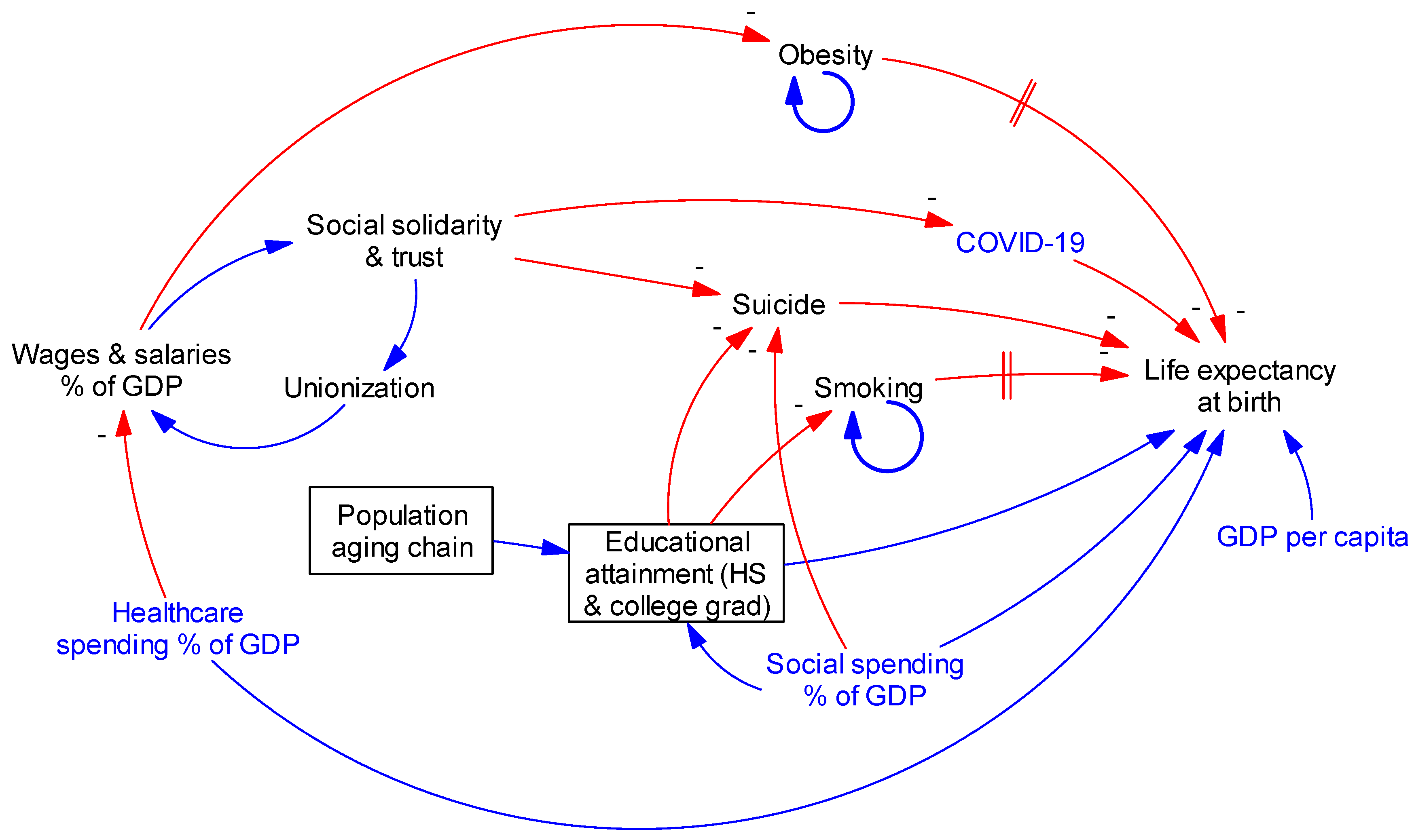
Figure 2.
Base run comparison to historical data for seven output variables SOURCE: Author’s model testing and data described in Table 1. NOTES: See Table 1 for variable definitions and data sources. Thick blue and green lines are from base run simulation. Thin red and black lines are historical data. Simulated LEB reflects assumed COVID-19 effect 2020-2024. Simulated social trust includes exogenous resurgence 1996-2005.
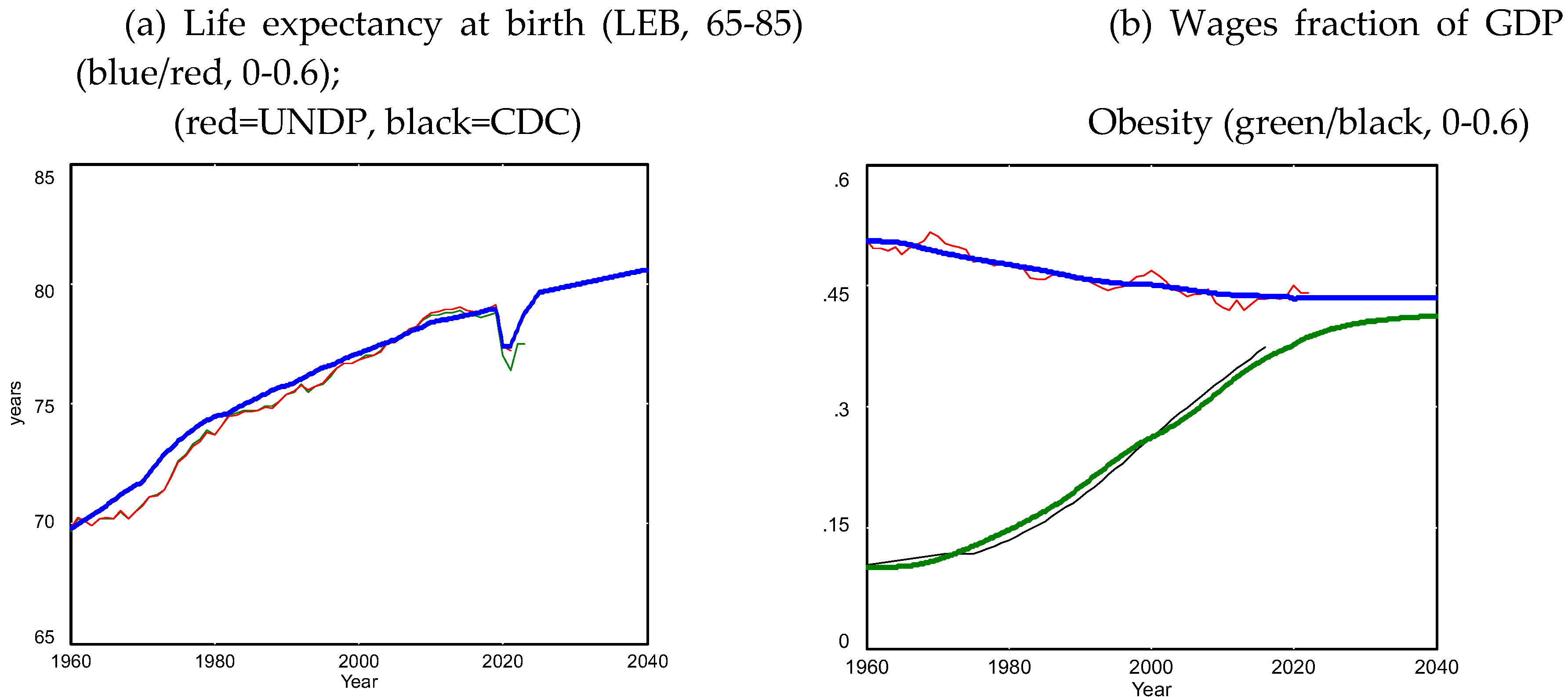
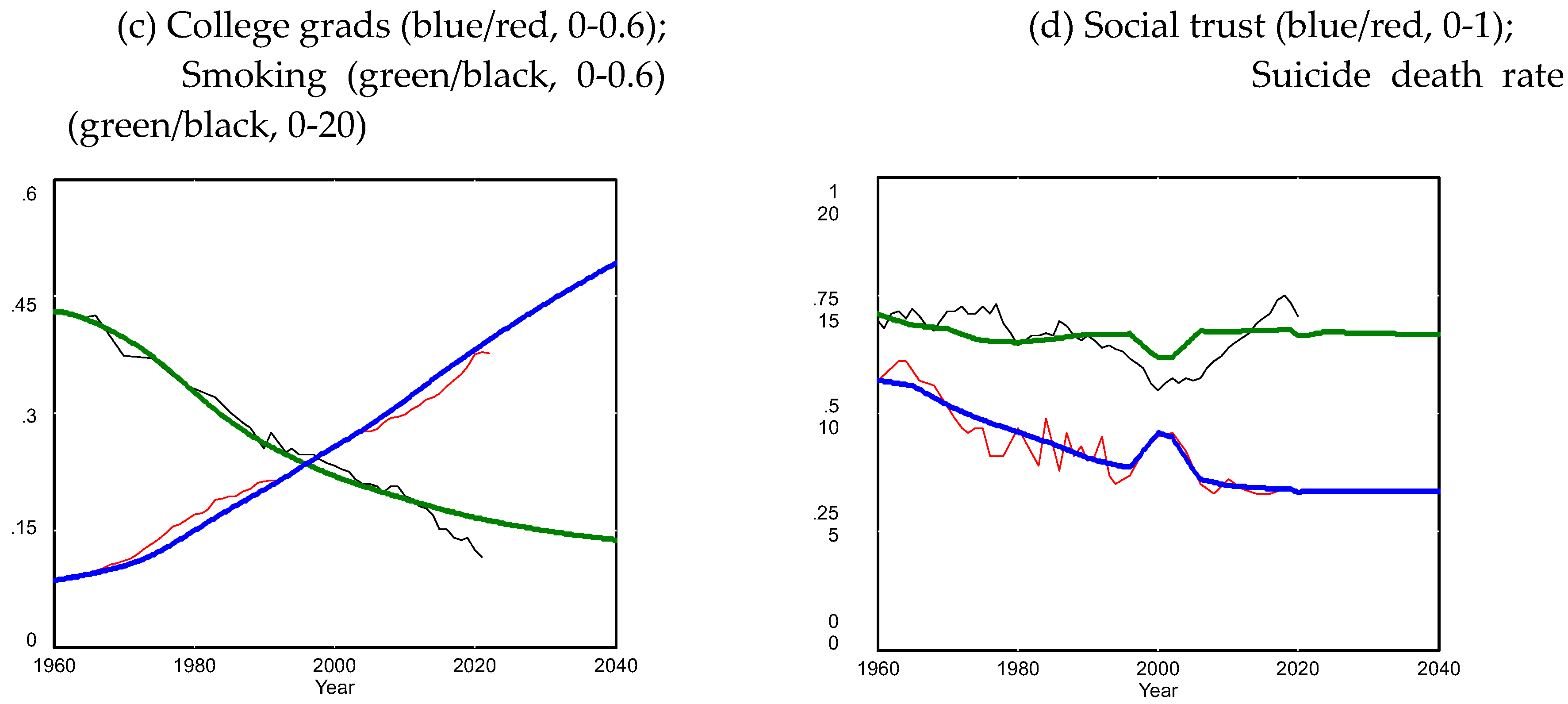
Figure 3.
Health care and social spending inputs for base run and counterfactual tests.SOURCE: Author’s model testing. NOTES: In the left-side graph, the blue line is from NHE through 2021 (=0.152), then assumed flat to 2040. The red line is for counterfactual tests CF1 and CF3; the health care spending fraction remains flat at 0.113 after 2000. In the right-side graph, the blue line is from OECD through 2021 (=0.227), assumed to ramp down to 0.20 by 2024, then flat to 2040. The green line is for counterfactual tests CF2 and CF3; the social spending fraction steps up to 0.24 after 2000 and remains there to 2040.
Figure 4.
Outputs from base run and three counterfactual tests. Scheme 2. and the red line is from CF1 and CF3. .In the top right graph for College Graduate Fraction, the blue line is from the base run and CF1, and the green line is from CF2 and CF3. In the lower right graph for LEB, the blue line is the base run, red is CF1, green is CF2, and black is CF3.
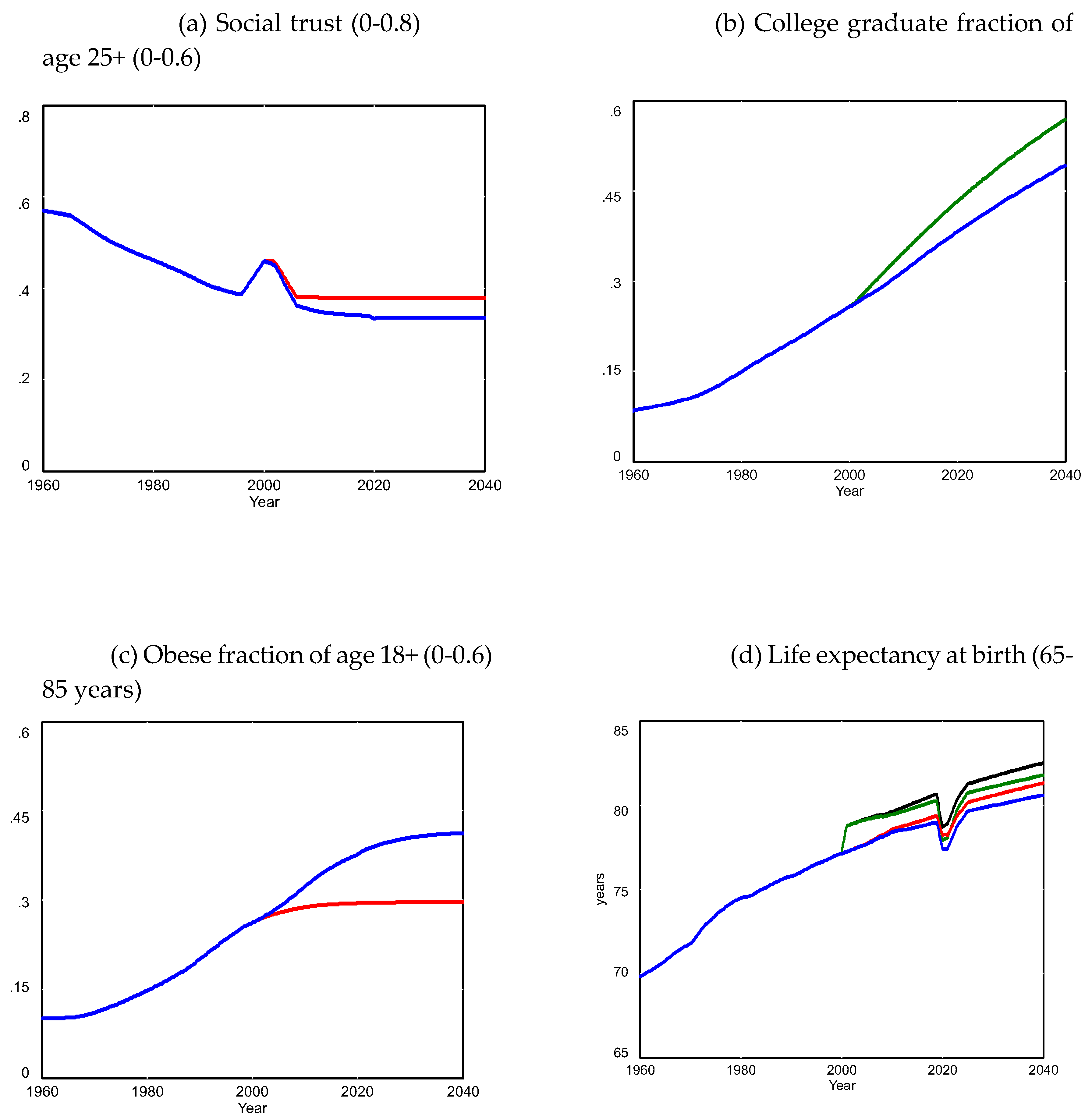

Table 1.
Data variables and years available..
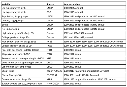
SOURCE: Author’s extraction of public data from multiple sources. NOTES: UNDP: United Nations Division of Population; 2022-2040 data are from UNDP’s medium variant projections. Age groups: 0-24, 25-64, 65-plus. CDC: US Centers for Disease Control and Prevention. UNDP and CDC estimates of LEB were generally very close (within 0.3 years) except for 2020 and 2021. NCES: National Center for Education Statistics (US Department of Education). FRED: Federal Reserve Economic Data (St. Louis Fed). NHE: National Health Expenditures database (from CMS: Centers for Medicare & Medicaid Services); government social spending data updated starting 1980 to include Medicare and Medicaid. OECD: Organization for Economic Cooperation & Development. WHO: World Health Organization (United Nations); obese: body mass index of 30 or greater. NHIS: National Health Interview Survey (CMS); current smoking was reported for 16 of the 32 years 1965-1996, with a maximum reporting gap of four years (1966-1978). Suicide death rate (WHO/OECD) is age standardized for OECD countries. Social trust (Roper/Putnam): Roper Center for Public Opinion Research, based on response to: “Generally speaking, would you say that most people can be trusted, or that you can’t be too careful in dealing with people?”, presented as time-series graph in Putnam/Garrett Figure 4.13 [26].
Table 2.
Base run goodness of fit to 12 historical data series.
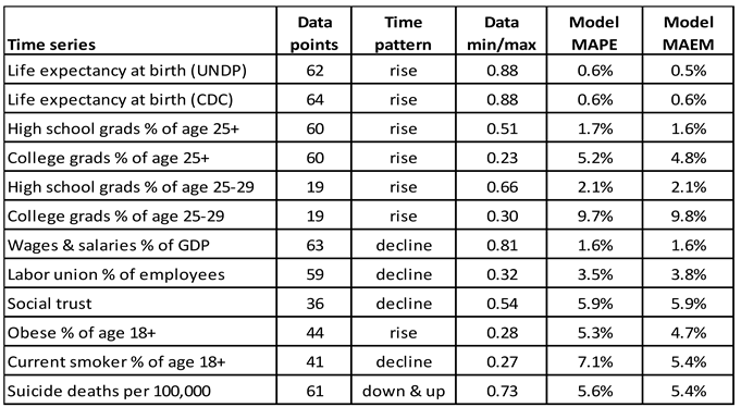
SOURCE: Author’s model testing, data described in Table 1, and author’s spreadsheet calculations. NOTES: “Data min/max” is the ratio of the minimum data point to the maximum; the smaller the ratio, the greater the data’s relative range. MAPE is the mean absolute percentage error of model compared with data. MAEM is the mean absolute error (MAE) divided by the mean of the data [16] absolute error divided by the mean of the data) metrics [16] are in all cases under 10% and under 1% for LEB specifically. The model indicates that declining LEB growth after 1980 was primarily the result of two factors: the growth of obesity, and the leveling off of growth in social spending.
Disclaimer/Publisher’s Note: The statements, opinions and data contained in all publications are solely those of the individual author(s) and contributor(s) and not of MDPI and/or the editor(s). MDPI and/or the editor(s) disclaim responsibility for any injury to people or property resulting from any ideas, methods, instructions or products referred to in the content. |
© 2024 by the authors. Licensee MDPI, Basel, Switzerland. This article is an open access article distributed under the terms and conditions of the Creative Commons Attribution (CC BY) license (http://creativecommons.org/licenses/by/4.0/).
Copyright: This open access article is published under a Creative Commons CC BY 4.0 license, which permit the free download, distribution, and reuse, provided that the author and preprint are cited in any reuse.


