Submitted:
18 October 2024
Posted:
22 October 2024
You are already at the latest version
Abstract
This study explores the intricate relationship between spectral irradiance variations and polar cap mean vertical total electron content (MVTEC) climatology, using ground-based GNSS measure-ments from the Thule station in the Arctic. The analysis focuses on understanding how different solar and magnetospheric processes drive changes in MVTEC patterns over a 2-year period. Three primary factors are identified as key drivers of MVTEC variations: (1) Russell-McPherron Effect: During equinoxes, enhanced energy transfer from the solar wind to the magnetosphere, governed by the Russell-McPherron effect, leads to increased MVTEC variability. This phenomenon arises due to the changing orientation of the solar magnetospheric coordinate system relative to the solar equatorial system, which affects the efficiency of energy deposition in the magnetosphere. As a result, higher ionospheric disturbances are observed during these periods, highlighting the sea-sonal influence of geomagnetic activity on polar cap TEC patterns. (2) Solar Irradiance Variations: The study identifies a strong correlation between fluctuations in solar EUV and F10.7, both proxies for solar irradiance, and the 27-day oscillations in MVTEC, especially during the summer months. These periodic variations are closely tied to the rotational behavior of the sun, suggesting a direct link between solar activity and ionospheric dynamics. The findings emphasize how solar spectral irradiance influences the ionization levels in the polar cap region, with implications for under-standing seasonal and short-term changes in the high-latitude ionosphere. (3) E-Layer Conductivity: Seasonal changes in the E-layer's conductivity also play a crucial role in modulating MVTEC variability. During summer, the presence of a conductive E-layer enhances cross-field plasma diffusion, leading to faster plasma decay and reduced MVTEC fluctuations. In contrast, the winter months are characterized by an insulating E-layer, which slows down plasma decay and allows F-layer structures to persist longer, resulting in increased MVTEC variability. This seasonal dis-parity underscores the importance of the E-layer's physical properties in shaping high-latitude ionospheric behavior. The findings of this study underscore the complex interplay between solar wind activity, solar irradiance, and ionospheric dynamics in shaping the observed patterns of polar cap MVTEC. By revealing the combined effects of solar and geomagnetic processes, this research contributes to a more comprehensive understanding of high-latitude ionospheric variability. Further investigation is needed to fully elucidate the mechanisms behind these interactions, particularly in terms of their implications for space weather forecasting and the operation of navigation systems in polar regions. Enhanced models that incorporate these insights can improve the prediction and mitigation of space weather effects on satellite-based technologies and communication systems.
Keywords:
ionosphere
; total electron content
; high-latitude ionosphere
; ionosphere climatology
; polar cap
1. Introduction
This study investigates the intricacies of sub-seasonal variations observed in the total electron content (TEC) of the northern polar cap ionosphere during the peak years (2013 and 2014) of Solar Cycle 24. By analyzing ground-based GNSS station measurements, we aim to elucidate the underlying mechanisms driving these variations.
A comprehensive understanding of these phenomena requires exploring the complex physical processes responsible for high-latitude ionospheric plasma generation and motion. At large scales, factors such as photoionization, particle precipitation, currents, and transport play a dominant role. While smaller-scale influences from natural sources like lightning exist, their impact on regional and global scales is negligible.
This study focuses on plasma density variations originating from solar photoionization. Solar radiation, the primary energy source driving photoionization and Earth's climate, undergoes long-term variations extensively studied by numerous researchers [1,2]. We concentrate on the wavelength segment of the solar irradiance spectrum responsible for ionizing the ionosphere, which encompasses extreme ultraviolet (EUV) and X-ray bands. Research has demonstrated a strong correlation between solar EUV flux and the F10.7 solar radio flux index, which is observable from the ground [3]. However, this correlation can weaken around solar minima [3].
To effectively measure solar EUV flux, spacecraft-based observations are essential. This parameter is a direct indicator of the main drivers behind TEC variations. Various ground-based, modeling, and satellite-based methods have been developed to observe ionospheric plasma and its relationship with driving factors [4]. Several models highlight the significant influence of parameters such as F10.7, solar zenith angle, seasonal changes, Kp index, magnetic latitude, solar wind pressure, interplanetary electric field, and interplanetary magnetic field on high-latitude electron density variations [5].
For this study, we leverage ground-based GNSS-TEC measurements complemented by digital ionosonde measurements. GNSS-TEC values are typically computed from data acquired by networks of ground stations, which can be global (e.g., [6]) or regional (e.g., the Greenland GPS Network (GNET) [7] and the Canadian CHAIN [8]).
This paper specifically focuses on long-term, single-station-derived mean vertical TEC (MVTEC) observations from Thule, Greenland, in relation to solar EUV irradiance and seasonal variations due to the Earth's rotational axis tilt relative to the Sun.
Various ground-based, modeling, and satellite-based methods have been developed to observe ionospheric plasma and its relationship with driving factors [4]. Several models highlight the significant influence of parameters such as F10.7, solar zenith angle, seasonal changes, Kp index, magnetic latitude, solar wind pressure, interplanetary electric field, and interplanetary magnetic field on high-latitude electron density variations [5].
For this study, we leverage ground-based GNSS-TEC measurements complemented by digital ionosonde measurements. GNSS-TEC values are typically computed from data acquired by networks of ground stations, which can be global (e.g., [6]) or regional (e.g., the Greenland GPS Network (GNET) [7] and the Canadian CHAIN [8]). This paper specifically focuses on long-term, single-station-derived mean vertical TEC (MVTEC) observations from Thule, Greenland, in relation to solar EUV irradiance and seasonal variations due to the Earth's rotational axis tilt relative to the Sun. The dynamics of plasma convection in the polar cap have been extensively studied [9,10,11,12,13,14]. These studies have revealed dependencies on diurnal, seasonal, and interplanetary magnetic field (IMF) factors. The sun is the primary driver of ionospheric variations. In the polar cap, plasma is in constant motion driven by the E x B drift, where the E-field configuration is influenced by the current solar wind's magnetic field and interactions with the neutral atmosphere. Previous studies [7,15] have presented TEC maps illustrating a unique feature of the polar cap ionosphere known as the tongue of ionization (TOI). The TOI involves plasma convection from the mid-latitude dayside into the night sector, and can fragment into isolated plasma irregularities (polar cap patches) during its movement. These patches exhibit higher convection speeds compared to lower-latitude plasma, often reaching ten times the typical equatorial values [16]. The generation, structure, and decay of polar cap patches have been extensively explored in the literature [10,17,18,19,20,21,22,23].
A critical plasma decay process in the polar cap F region is the scale-size decay of F-region instabilities, which is influenced by the presence of a highly conductive E region due to enhanced magnetic field plasma diffusion processes [24]. This results in distinct GNSS-TEC variations depending on the sunlit status of the related flux tubes and the season. For instance, 10 km scale size plasma irregularities can persist for days, while 1 km scale irregularities decay a hundred times faster. Even smaller scales, such as 100 meters, decay rapidly, although they may still exist in the polar cap ionosphere due to other factors [25,26]. When a sunlit portion of the polar cap ionosphere contains irregularities, photoionization fills in the low plasma density volumes between patches, leading to a smoother F region plasma as observed in GNSS-TEC measurements. This effect dominates during daylight hours and throughout the summer when the polar cap ionosphere remains continuously sunlit due to the Earth's axis tilt [21,23,24]. Another phenomenon influencing polar cap ionospheric dynamics is the Russell-McPherron effect, described in [14]. This mechanism modulates the energy extracted from storm-producing plasma in the solar wind throughout the year, resulting in a 40% increase in the average energy input during equinoxes compared to solstices. The formation and occurrence of polar cap patches depend on the interactions between the solar wind, geomagnetic field, and energy input from the solar wind, among other factors. Consequently, the Russell-McPherron effect directly impacts these patches [27,28].
2. Materials and Methods
The single GNSS ground-station employed in this study is located at Thule (also called Qaanaaq), in northwestern Greenland (76.53°N, 68.78°W), as depicted in Figure 1. This ground-station was one of the first operational permanent GNSS receivers in the network now known as the Greenland GNSS Network (GNET). Thule holds scientific significance due to its location in the deep polar cap region, which corresponds to open geomagnetic flux tubes [29]. The ionized portion of the upper atmosphere over this region is also referred to as the high-latitude ionosphere when the auroral oval, the boundary between open and closed flux tubes, is included. The high-latitude ionosphere and the polar cap magnetosphere have been extensively studied due to their unique physical processes and features, with numerous observations conducted from various ground stations located at Thule. This enables the comparison of collocated measurements and the utilization of conducted experiments in this area as a basis for the present study.
[21,23] reported irregularity structures and their frequency spectra from the polar cap, derived from measurements conducted at Thule using 250 MHz transmissions from quasi-stationary satellites. They also reported phase and intensity scintillation variations for several years. These findings will be compared to our observations and interpreted later in this article.
A digital ionosonde operating in Thule provided relevant measurements until the second half of August 2014. This data offers a good temporal overlap with our GNSS-TEC measurements. Based on ionosonde measurements, bottom-side electron density (Ne) profiles can be reconstructed, while the topside is modeled with a fitted Chapman profile. Measurements were collected every 15 minutes. Ionosonde-derived Ne profiles can be compared to TEC measurements after integration. For further details on this method and its validation, refer to [7,30].
The two main geomagnetic indices used in this study are the disturbance storm-time index (Dst) [31] and the auroral electrojet index (AE) [32]. Dst measures the intensity of the ring current, while AE provides information about auroral zone magnetic activity. Both indices can be used as indicators of specific ionospheric activities [33]. We obtained Dst and AE data from NOAA's Space Physics Data Facility (SPDF) website (https://omniweb.gsfc.nasa.gov/form/dx1.html ).
Another index used in this study is the polar cap north (PCN) index [34]. This index is computed from single-station magnetic measurements taken by a ground-based magnetometer located in Thule. Variations and values of the PCN index indicate energy input changes into the polar cap region [7]. Larger PCN variations and values are typically observed during geomagnetic storms and exhibit seasonal and solar cycle dependences. PCN values were acquired from the Polar Cap Magnetic Index website [34].
Solar EUV (extreme ultraviolet, from 0.01 to 0.1 μm wavelength) radiation is the primary driver of Earth's ionosphere formation, although solar X-rays can also ionize atmospheric species [35]. In this study, we employed EUV flux measurements from NASA's Solar Radiation and Climate Experiment (SORCE) satellite [36]. SORCE continuously measures the sun's total solar irradiance (TSI) and spectral solar irradiance (SSI). It accomplishes this using four instruments: Total Irradiance Monitor (TIM), Solar Stellar Irradiance Comparison Experiment (SOLSTICE), Solar Irradiance Monitor (SIM), and Soft X-ray Ultraviolet Photometer System (XPS).
Since SORCE data has significant gaps, we used F10.7 solar radio flux data as a proxy for EUV measurements in the figures. The solar radio flux at 10.7 cm (2800 MHz), or simply the F10.7 index, is another indicator of solar activity. These radio emissions originate from the upper chromosphere and lower corona of the solar atmosphere. The F10.7 index correlates well with sunspot number and several UV and visible solar irradiance records. The F10.7 data was acquired from NOAA’s Space Physics Data Facility (SPDF) website (https://omniweb.gsfc.nasa.gov/form/dx1.html). The SORCE instruments together provide measurements of the full-disk spectral solar irradiance (SSI) from 0.1 nm to 2400 nm, but the frequency range between 34 to 115 nm is not covered. The resolution of the SSI measurements (from 115 nm to 310 nm) is 1 nm, and from 310 nm to 2400 nm is varying from 1 to 34 nm. The irradiance data represents measurements at a mean solar distance of 1 astronomical unit (AU) with units of W/m2/nm. The SORCE data can be acquired from the University of Boulder Colorado website (https://lasp.colorado.edu/home/sorce/data/ ).
TEC values were derived from Thule-based GNSS receiver (THU3) using a single-layer ionospheric model [37]. The potential ionospheric pierce points (IPPs) spanned a geographic range of approximately 150°W to 10°E longitude and 63°N to 90°N latitude, employing a 10° elevation cutoff angle (see Figure 1). The 1-Hz sampled data was processed by JPL's Global Ionospheric Maps (GIMs) [38], resulting in calibrated VTEC values and their IPP coordinates, down-sampled to 5 minutes. Calibrated VTEC values were computed by estimating satellite and receiver differential biases [6]. Subsequently, these VTEC values were further processed to obtain mean VTEC (MVTEC) values [30] for a total period of four years (2012-2015).
MVTEC values represent a single value measured in TEC units (TECU, 1 TECU = 1016 electrons m-2) over the station and calculated as the mean of all observed VTEC values for a given epoch. This single value can be interpreted as a smoothed ionosphere single layer that filters out smaller ionospheric irregularities. It primarily represents the overall trend in the region, which is more likely to be attributed to solar ionization or other large-scale phenomena, such as N2 upwelling due to atmospheric heating resulting from a geomagnetic storm. For further details on MVTEC calculations and its dependence on geomagnetic storms in the polar cap, refer to [7]. Notably, due to the down-sampling of VTEC data from 1 Hz to 5 minutes, all MVTEC time series also had values every 5 minutes.
Figure 1 also illustrates the estimated geographic positions of the IPPs. Each IPP arc corresponds to the point where the signal path from a specific GPS satellite crosses the ionospheric single-layer model shell, as seen from the Thule site. At any epoch, there are usually around 10 to 12 IPPs. The VTEC value for each of these IPPs at a given time contributes equally to the MVTEC.
The validation of MVTEC values acquired from the Thule site was conducted by comparing these results with data from 35 GNET stations, processed using Bernese 5.0 software (for details on how Bernese computes VTEC values, see [39]). The Bernese software calculates VTEC values on a regular grid, and these values were averaged to produce a quantity comparable to MVTEC. A comparison between the Thule MVTEC and the Bernese-averaged VTEC is shown in Figure 2. Additionally, the 35-station average MVTEC results were compared with the ionospheric TEC product from the Center for Orbit Determination in Europe (CODE), revealing a very strong correlation and minimal offset. CODE’s ionospheric products are accessible at https://ftp.aiub.unibe.ch.
Figure 2 highlights a striking similarity between the two independently computed electron densities. It is important to note that the Bernese output has a time resolution of 1 hour, while the JPL GIM data has a 5-minute time resolution. As a result, the Bernese time series (blue line) appears smoother than the JPL GIM time series (red line), with smaller irregularities and rapid variations being absent in the Bernese data.
The relationships among MVTEC time series, critical frequency profiles, and various geomagnetic indices were also examined. Electron density data derived from digital ionosondes provided insights into the altitudes where the most notable changes occur. The relationship between the critical frequency (fc) and maximum plasma density (Ne,max) is defined by (Reinisch et al., 2009). A comparison between MVTEC and the integrated critical frequency revealed a strong correlation. The methodology for comparing GNSS-TEC with ionosonde-derived Ne was detailed in [7]. The good agreement between GNSS-TEC and ionosonde-derived integrated plasma density time series serves as additional independent validation of MVTEC as a reliable measure of ionospheric electron density variations. However, when MVTEC was compared with the Dst and AE indices, no significant relationship was observed (Figure 3), suggesting that short-term geomagnetic activity has no substantial long-term impact on polar cap TEC climatology. MVTEC was then compared with the PCN index (Figure 3), which displayed distinct features not aligned with MVTEC, showing higher amplitudes during summer and lower amplitudes during winter. These fluctuations are linked to changes in Earth's inclination relative to the solar wind, as the solar wind energy input increases when the northern polar cap faces the sun (Figure 3, (c)). Remarkably, the PCN does not show heightened activity near the equinoxes, contrary to what the Russell-McPherron effect would predict.
3. Results
This study identified three primary factors influencing the MVTEC time series features, which are illustrated in Figure 3: (1) solar wind, (2) solar EUV (and higher frequency) radiation, and (3) a combination of solar EUV and E-layer-related mechanisms.
The observed semi-annual variation in geomagnetic activity, as described by [14], is attributed to the varying angle between the southward component of the interplanetary magnetic field (IMF) and Earth's magnetosphere. This results in the Russell-McPherron effect, which causes increased geomagnetic activity near the equinoxes due to enhanced energy input from the solar wind. Figure 3 demonstrates high MVTEC variability around these periods, corresponding to approximately 40% more solar wind energy being deposited into the magnetosphere than during the solstice months, which leads to increased disturbances in the ionosphere.
Figure 3(a) shows several datasets from 2013 and 2014, with the MVTEC time series alongside OMNI-derived sunspot numbers, indicating a strong correlation between sunspot numbers and the ~27-day TEC fluctuations. This correlation is more apparent during the summer months when the ionosphere is smoother, reducing noise-like features. The F10.7 index, a proxy for solar EUV radiation, is presented in Figure 3(b), while the PCN index, representing solar wind energy input into the polar cap, is shown in Figure 3(c). Figure 3(d) and 3(e) display the AE and Dst indices, respectively, highlighting geomagnetic storms without showing significant influence on TEC climatology at the timescale presented.
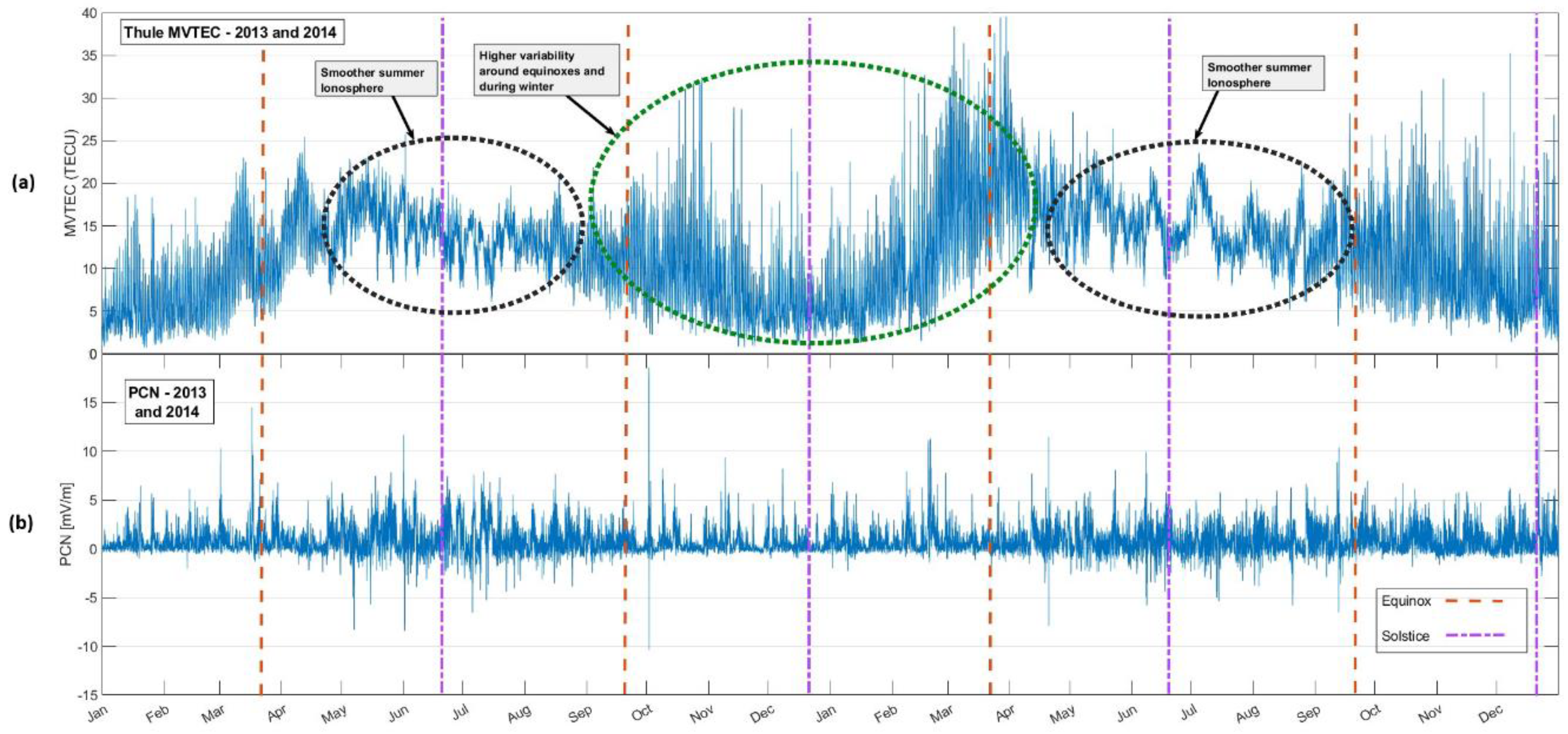
Additionally, the MVTEC time series reveals features that cannot be entirely attributed to solar wind-magnetosphere interactions. The data indicate that solar irradiance plays a significant role, especially during summer when the polar cap ionosphere receives continuous ionizing radiation, resulting in higher TEC values. Figure 3 and Figure 4 suggest that the greatest MVTEC variability occurs between the fall and spring equinoxes, including the entire winter season. This variability can be linked to the reduced conductivity of the E layer during winter, allowing plasma structures to persist longer, thus contributing to increased disturbances.
The MVTEC anomalies have a periodicity slightly shorter than a month, hinting at a correlation with the 27-day solar rotation. Analysis of data from the Qaanaaq digital ionosonde for the summer months of 2014 supports this, showing that most ionization occurs in the F2 region of the ionosphere. Figure 3(a) illustrates a slight phase offset, with MVTEC rising 2-4 days before sunspot numbers increase. This offset is also evident with the F10.7 index (Figure 3(b)).
4. Discussion
The results show that semi-annual geomagnetic variations, primarily influenced by the Russell-McPherron effect, lead to increased disturbances around the equinoxes due to enhanced energy transfer from the solar wind to the magnetosphere. This process explains the highly disturbed segments of the MVTEC time series observed during these periods. Although the exact mechanism of energy transfer to the polar cap ionosphere, as suggested by [14], is not fully understood, it highlights the need for further research incorporating solar wind parameters, SuperDARN maps, GNSS-derived TEC maps, and satellite data.
The correlation between sunspot numbers, the F10.7 index, and the ~27-day TEC fluctuations suggests that solar rotation plays a significant role. While models of total solar irradiance do not fully account for these anomalies, the EUV portion, as represented by the F10.7 index, shows strong alignment with MVTEC data when adjusted for phase offset. However, this correlation alone does not explain all observed variations, indicating that other processes, such as differential solar rotation (where different latitudes on the sun's surface rotate at varying rates), are also at play, as detailed in [45].
Additional features in the MVTEC time series (Figure 3) suggest influences beyond solar wind-magnetosphere interactions, driven by variations in solar irradiance. For example, during summer months, the polar cap ionosphere receives more ionizing radiation, resulting in higher TEC values. Additionally, periods when the sun remains above the horizon lead to continuous ionization throughout the day. Given these factors, one might expect a quasi-sinusoidal pattern in the MVTEC data, peaking in summer and dipping in winter. However, Figure 3 and Figure 4 reveal a more complex scenario. While some anomalies may be linked to the Russell-McPherron effect, others appear to have different underlying causes. Specifically, Figure 3(a) shows that the greatest MVTEC variability occurs between the fall and spring equinoxes, including the entire winter season, a trend also evident in Figure 4. This variability begins around the equinoxes (due to the Russell-McPherron effect) and is only slightly reduced by the drop in E-layer conductivity during winter, caused by decreased solar EUV over the polar cap. During winter, plasma structures drifting from lower latitudes persist longer, contributing to the observed increase in MVTEC disturbances.
The period of MVTEC anomalies appears to be slightly shorter than a month, possibly indicating a correlation with the 27-day solar rotation. For details on the differential rotation of the sun, see, for example, [44]. To confirm that this 27-day electron density variation also exists in other independent measurements, data from the Qaanaaq digital ionosonde was analyzed. Critical frequency profiles were calculated for the summer months (June, July, and August) of 2014, showing that most of the ionization occurred in the F2 region of the ionosphere.
Figure 3 (a) illustrates the connection between sunspot numbers and MVTEC. The quasi-periodic 27-day anomalies are slightly out of phase with sunspot numbers, as the MVTEC tends to rise 2-4 days before an increase in sunspot numbers becomes evident. The same phase offset is observed with the F10.7 index (Figure 3 (b)). Although a model considering only total solar irradiance does not fully account for the 27-day anomaly, the EUV portion of solar irradiance (or its proxy index F10.7), when adjusted for the phase offset, correlates well with MVTEC, showing a significant relationship. However, it's also evident that other factors must be at play, as sunspot numbers do not account for all variations in EUV and the F10.7 index. Still, these observations suggest that the ~27-day MVTEC variations are tied to solar rotation. As the sun rotates, the Earth's ionosphere receives varying amounts of ionizing radiation, partly depending on the number of sunspots present. [45] explains the phenomenon of solar differential rotation, where different latitudes of the solar surface rotate at varying periods. The rotation period is shortest (~24.47 days) near the equator and longest (~35 days) near the poles, implying differential rotation of sunspots as well.
Another significant aspect is based on the model by [24], known as the Horizontally Structured F-region Plasma Decay Model (FPDM). This model aims to explain the physical mechanisms behind the decay of polar cap F-layer structures, considering the effects of a conducting E layer. Both highly structured F-layers and conducting E-layers are common features of the Arctic ionosphere and fundamental components of the FPDM. Other authors, including [7,8,46], have also described these ionospheric structures and large-scale, high-latitude phenomena, which include TOI, polar patches, polar holes, ionization troughs, auroral ionization enhancements, and electron/ion temperature hotspots. The occurrence and characteristics of these features depend on various factors, such as convection patterns, local time, season, IMF/solar wind parameters, and even the solar cycle [47]. It's crucial to note that the Arctic ionosphere is not an isolated system, and significant plasma transport from lower latitudes can occur. Plasma originating from mid-latitudes can be transported anti-sunward into and across the polar cap, primarily during southward IMF, when multi-cell convection pattern forms over the polar cap [48]. This plasma source could be storm-enhanced density (SED) plumes, which are observed between the post-noon and pre-midnight sectors as distinct regions of enhanced plasma densities. Although several researchers, including [48,49,50], have studied SED plumes, they are not yet fully understood and are beyond the scope of this work.
The complete mathematical derivation of the FPDM is available in [24], but a brief summary is provided here. Several simplifying assumptions are made: (a) The E layer is modeled as a uniform, conductive medium using the height-integrated Pedersen conductivity, denoted as . (b) Ne(z, r, t). This serves as a reasonable approximation for the summer polar cap ionosphere. (b) The electron density Ne(z, r, t) is expressed as a product Z(z)N(r, t), where the vector r is perpendicular to the magnetic field B, which is assumed to be vertical within the polar cap. (c) The electric field E is considered independent of altitude, z, due to the high vertical conductivity present. (d) Quasi-neutrality is assumed, meaning Ne = Ni = N. Based on these assumptions, and by incorporating the continuity equations for ions and electrons, [24] derived an equation that establishes the relationship between the electric field E and the density gradient ∇N, accounting for the influence of the conductive E layer.
here, and represent the height-integrated ion and electron conductivities, respectively. The term denotes the charge of the species, while and are the ion and electron ambipolar diffusion coefficients, with ⊥ indicating a direction perpendicular to the magnetic field. These diffusion coefficients are derived from the diffusion tensors. Ambipolar diffusion occurs when a polarization electric field arises, preventing significant charge separation between ions and electrons; thus, both move together under external forces within the ionospheric plasma. When the E layer acts as an insulator, such as during winter in the polar cap, Equation (1) can be simplified to a more straightforward form:
here, KB represents the Boltzmann constant, and Ti denotes the ion temperature as detailed in [24,47]. With this information, predictions from the FPDM can be compared against the MVTEC observations depicted in Figure 4. Based on Equations (1) and (2), different ionospheric patterns are anticipated during winter (when the polar cap receives little to no solar photoionization) and summer (when the polar cap ionosphere remains sunlit for most or all of the day). Additionally, there should be a transition phase around the equinoxes, where the effects discussed in [14] are also at play.
During winter, the polar cap generally lacks a highly conductive E layer, allowing larger patches (irregularities around 10 km) to persist against diffusion for days, enabling them to travel across the polar cap multiple times. On smaller scales, around 1 km, the decay rate is significantly higher, leading to only a few hours of survival at best. At even smaller scales (hundreds of meters), diffusion acts so quickly that these structures should dissipate swiftly, even with an insulating E layer, making their presence unlikely in observations. However, the detection of smaller structures suggests additional processes not accounted for by the FPDM [24]. Comparing the model's predictions to actual data, Figure 4 reveals significant MVTEC variations during winter, likely due to fast-moving patches that persist over extended periods and do not decay rapidly. It's important to note that MVTEC mainly detects larger structures, which, according to FPDM, exhibit slow decay during the winter months.
Beyond the FPDM model, another related phenomenon discussed in [51] is relevant. During summer or whenever flux tubes enter sunlit regions, the low-density gaps (holes) between patches (areas of enhancement) can be "filled in" by photoionization. If sufficient time is available, this process leads to a more uniform plasma density [24,51]. To understand this effect, it's essential to explore the connection between amplitude scintillations and TEC variations. Previous studies [7,16,52] have demonstrated a non-linear correlation between amplitude scintillations and the Rate of TEC Index (ROTI), which is calculated based on changes in TEC (for precise equations, see [16]). Thus, strong variations in MVTEC data imply that phase scintillations would be more pronounced along the same signal path. Consequently, it aligns with the findings in [51], which indicate that during summer, the polar cap ionosphere typically shows reduced scintillations due to this "filling in" effect, while during equinox periods, scintillations are ten times more likely. According to [51], statistically, the highest scintillations occur just after the equinoxes, but they remain consistently elevated throughout winter (Figure 4). This suggests that the Russel-McPherron effect may have a greater influence on polar cap scintillations than the reduced decay caused by the insulating E layer.
5. Conclusions
This study has explored three distinct mechanisms that influence the primary characteristics of a 2-year set of regional electron density measurements from the Thule GNSS site in the Arctic. The findings highlight the complex interplay between solar and magnetospheric processes in shaping the behavior of the polar cap ionosphere. The main conclusions are summarized as follows:
- Russell-McPherron Effect: The significant MVTEC variability observed around the equinoxes is primarily attributed to the Russell-McPherron effect, which results in a 40% increase in energy transfer from the solar wind to the magnetosphere during these periods. This enhanced energy input leads to heightened ionospheric disturbances in the Arctic region. The findings emphasize how seasonal and solar wind conditions converge to drive these semi-annual variations, underscoring the need for further research into the mechanisms governing this energy transfer process.
- SSI EUV-Related 27-Day Variations: Throughout the study period, MVTEC data revealed a consistent ~27-day oscillation with an amplitude of 10-15 TECU. These variations, more pronounced during summer, are closely linked to the smooth ionospheric conditions caused by continuous solar photoionization. The correlation with solar EUV, F10.7, and sunspot numbers points to the influence of solar rotation, demonstrating how periodic changes in solar activity propagate through the magnetosphere to affect the ionosphere. This underscores the importance of understanding solar spectral irradiance as a driver of high-latitude ionospheric dynamics.
- E-Layer Conductance and FPDM: The variability in the MVTEC time series is markedly lower in the summer compared to winter and equinox periods. This behavior is well explained by the FPDM model proposed by [24], which attributes the seasonal differences to changes in E-layer conductance. During summer, the presence of a conductive E layer increases the cross-field plasma diffusion rate in the F layer, leading to more stable ionospheric conditions. Conversely, in winter, the E layer acts as an insulator, slowing down plasma decay and allowing structures to persist longer, resulting in greater MVTEC variability. This seasonal contrast emphasizes how changes in E-layer properties contribute to the overall behavior of the polar cap ionosphere.
The study has provided valuable insights into the behavior of the Arctic ionosphere, but it also highlights areas for future research. Understanding the detailed mechanisms of energy transfer between the solar wind and the polar cap ionosphere, particularly during equinox periods, requires a more comprehensive analysis using integrated datasets, including SuperDARN convection maps, GNSS-derived TEC maps, and satellite-based observations. Additionally, exploring the underlying physics of the ~27-day variations in relation to differential solar rotation could offer further insights into how solar phenomena impact the Earth's upper atmosphere. Further investigation into the seasonal dynamics of E-layer conductance, including its variability under different geomagnetic conditions, could also improve models like FPDM and enhance our predictive capabilities for ionospheric behavior in the polar regions.
Overall, these findings not only deepen our understanding of polar cap ionospheric dynamics but also have broader implications for space weather forecasting and navigation systems operating in high-latitude environments. As the impact of solar and geomagnetic activity on communication and navigation continues to grow, the insights provided by this study will be crucial for developing more robust models and mitigation strategies.
Author Contributions
Conceptualization, Tibor Durgonics; methodology, Tibor Durgonics and Attila Komjathy; software, Tibor Durgonics and Attila Komjathy; validation, Tibor Durgonics; formal analysis, Tibor Durgonics, Attila Komjathy and Per Høeg; investigation, Tibor Durgonics, Attila Komjathy and Per Høeg; resources, Tibor Durgonics and Attila Komjathy; data curation, Tibor Durgonics; writing—original draft preparation, Tibor Durgonics; writing—review and editing, Tibor Durgonics, Attila Komjathy and Per Høeg; visualization, Tibor Durgonics; supervision, Attila Komjathy and Per Høeg; project administration, Tibor Durgonics; funding acquisition, Tibor Durgonics and Per Høeg. All authors have read and agreed to the published version of the manuscript.
Funding
This research was supported in part by the Technical University of Denmark and the NOAA cooperative agreement NA22OAR4320151.
Data Availability Statement
The authors acquired the RINEX data used for the Thule ground-station TEC and the Greenlandic regional ground-based TEC processing in the study from the Danish National Space Institute (DTU Space, Technical University of Denmark, this data is now openly available from the UNAVCO GPS/GNSS Data website at via https://www.unavco.org/data/gps-gnss/gps-gnss.html. The Dst and AE data were acquired from NOAA’s SPDF website at https://omniweb.gsfc.nasa.gov/form/dx1.html. PCN values were acquired from the Polar Cap Magnetic Index website at https://pcindex.org, maintained by the Arctic and Antarctic Research Institute and the Technical University of Denmark, DTU Space. The SORCE data can be acquired from the University of Boulder Colorado website at https://lasp.colorado.edu/home/sorce/data/. The F10.7 data was acquired from NOAA’s Space Physics Data Facility (SPDF) website at https://omniweb.gsfc.nasa.gov/form/dx1.html. TEC product from the Center for Orbit Determination in Europe (CODE), the CODE ionospheric products are available from https://ftp.aiub.unibe.ch. 5.2 of the Bernese software used for Greenlandic TEC time-series calculations is preserved at http://www.bernese.unibe.ch/, available via research or commercial license and developed openly at http://www.bernese.unibe.ch/order/. JPL GIM software used for processing Thule RINEX files is preserved https://ott.jpl.nasa.gov/software, available via free research license and developed openly at https://ott.jpl.nasa.gov/software.
Acknowledgments
The authors wish to thank the Danish National Space Institute (DTU Space, Technical University of Denmark) for the Thule GNSS ground station data.
Conflicts of Interest
The authors declare no conflict of interest. The funders had no role in the design of the study; in the collection, analyses, or interpretation of data; in the writing of the manuscript; or in the decision to publish the results.
References
- Yeo, K. L., N. 201A. Krivova, S. K. Solanki and K. H. Glassmeier (2014), Reconstruction of total and spectral solar irradiance from 1974 to 2013 based on KPVT, SoHO/MDI, and SDO/HMI observations, A&A, Vol. 570.
- Willson, R. C. and H. S. Hudson (1991), The Sun's luminosity over a complete solar cycle, Nature. 351 (6321): 42–4. [CrossRef]
- Chen, Y., L. Liu, and W. Wan (2011), Does the F10.7 index correctly describe solar EUV flux during the deep solar minimum of 2007–2009? J. Geophys. Res., 116, A04304. [CrossRef]
- Wood, A.G., Alfonsi, L., Clausen, L. B. N., Jin, Y., Spogli, L., Urbář, J., Rawlings, J.T.., Whittaker, I. C.., Dorrian, G. D., Høeg, P., Kotova, D., Cesaroni, C., Cicone, A., Miedzik, J., Gierlach, E., Kochańska, P., Wojtkiewicz, P., Shahtahmassebi, G., & Miloch, W. J. (2022). Variability of Ionospheric Plasma: Results from the ESA Swarm Mission. Space Sci Rev 218, 52. [CrossRef]
- Spogli L., Y. Jin, J. Urbár, A. G. Wood, E. E. Donegan-Lawley, L. B. N. Clausen, G. Shahtahmassebi, L. Alfonsi, J. T. Rawlings, A. Cicone, D. Kotova, C. Cesaroni, P. Høeg, G. D. Dorrian, L. Nugent, S. Elvidge, D. Themens, M. J. B. Aragón, J. M. Redondo, P. Wojtkiewicz, and W. J. Miloch (2023). Statistical Models of the Variability of Ionospheric Plasma in the Topside Ionosphere: Part 2: Performance assessment. J. Space Weather Space Clim. [CrossRef]
- Komjathy, A., L. Sparks, B. D. Wilson, and A. J. Mannucci (2005), Automated daily processing of more than 1000 ground-based GPS receivers for studying intense ionospheric storms, Radio Sci., 40, RS6006. [CrossRef]
- Durgonics, T., A. Komjathy, O. Verkhoglyadova, E. B. Shume, H.-H. Benzon, A. J. Mannucci, M. D. Butala, P. Høeg, and R. B. Langley (2017), Multiinstrument observations of a geomagnetic storm and its effects on the Arctic ionosphere: A case study of the 19 February 2014 storm, Radio Sci., 52. [CrossRef]
- Prikryl, P., et al. (2016), GPS phase scintillation at high latitudes during the geomagnetic storm of 17–18 March 2015, J. Geophys. Res. Space Physics, 121, 10,448–10,465. [CrossRef]
- Watson, C., P. T. Jayachandran, and J. W. MacDougall (2016), GPS TEC variations in the polar cap ionosphere: Solar wind and IMF dependence, J. Geophys. Res. Space Physics, 121, 9030–9050. [CrossRef]
- Prikryl, P., P. T. Jayachandran, R. Chadwick, and T. D. Kelly (2015), Climatology of GPS phase scintillation at northern high latitudes for the period from 2008 to 2013, Ann. Geophys., 33, 531–545. [CrossRef]
- Jayachandran, P. T., C. Watson, I. J. Rae, J. W. MacDougall, D. W. Danskin, R. Chadwick, T. D. Kelly, P. Prikryl, K. Meziane, and K. Shiokawa (2011), High-latitude GPS TEC changes associated with a sudden magnetospheric compression, Geophys. Res. Lett., 38, L23104. [CrossRef]
- Kullen, A., J. A. Cumnock, and T. Karlsson (2008), Seasonal dependence and solar wind control of transpolar arc luminosity, J. Geophys. Res., 113, A08316. [CrossRef]
- Ruohoniemi, J. M., and R. A. Greenwald (2005), Dependencies of high-latitude plasma convection: Consideration ofinterplanetary magnetic field, seasonal, and universal time factors in statistical patterns,J. Geophys. Res.,110, A09204. [CrossRef]
- Russell, C. T., and R. L. McPherron (1973), Semiannual variation of geomagnetic activity, J. Geophys. Res., 78(1), 92–108. [CrossRef]
- Foster, J. C., et al. (2005), Multiradar observations of the polar tongue of ionization, J. Geophys. Res., 110, A09S31. [CrossRef]
- Jacobsen, K. S. (2014), The impact of different sampling rates and calculation time intervals on ROTI values, J. Space Weather Space Clim., 4, 9. [CrossRef]
- Hosokawa, K., J. I. Moen, K. Shiokawa, and Y. Otsuka (2011), Motion of polar cap arcs,J. Geophys. Res.,116,A01305. [CrossRef]
- MacDougall, J. W., and P. T. Jayachandran (2007), Polar patches: Auroral zone precipitation effects, J. Geophys. Res., 112, A05312. [CrossRef]
- Moen, J., N. Gulbrandsen, D. A. Lorentzen, and H. C. Carlson (2007), On the MLT distribution of F region polar cap patches at night, Geophys. Res. Lett., 34, L14113. [CrossRef]
- Pedersen, T., B. Fejer, R. Doe, and E. Weber (2000), An incoherent scatter radar technique for determining two-dimensional horizontal ionization structure in polar cap F region patches, J. Geophys. Res., 105, 10,637–10,655.
- Basu, S., S. Basu, P. K. Chaturvedi, and C. M. Bryant Jr. (1994), Irregularity structures in the cusp/cleft and polar cap regions, Radio Sci., 29(1), 195–207. [CrossRef]
- Kivanç, Ö., and R. A. Heelis (1998), Spatial distribution of ionospheric plasma and field structures in the high-latitude F region, J. Geophys. Res., 103(A4), 6955–6968. [CrossRef]
- Basu, S., S. Basu, E. MacKenzie, and H. E. Whitney (1985), Morphology of phase and intensity scintillations in the auroral oval and polar cap, Radio Sci., 20(3), 347–356. [CrossRef]
- Vickrey, J. F., and M. C. Kelley (1982), The effects of a conducting E layer on classical F region cross-field plasma diffusion, J. Geophys. Res., 87(A6), 4461–4468. 4461. [CrossRef]
- van der Meeren, C., K. Oksavik, D. A. Lorentzen, M. T. Rietveld, and L. B. N.Clausen (2015), Severe and localized GNSS scintillation at the poleward edge of the nightside auroral oval during intense substorm aurora, J. Geophys. Res. Space Physics, 120, 10,607–10,621. [CrossRef]
- Fejer and Kelley, 1980. B.G. Fejer, M.C. Kelley. Ionospheric irregularities. Rev. Geophys. Space Phys., 18 (1980), p. 401.
- Prikryl, P., Gillies, R. G., Themens, D. R., Weygand, J. M., Thomas, E. G., and Chakraborty, S. (2022) Multi-instrument observations of polar cap patches and traveling ionospheric disturbances generated by solar wind Alfvén waves coupling to the dayside magnetosphere, Ann. Geophys., 40, 619–639. [CrossRef]
- Kagawa, A., K. Hosokawa, Y. Ogawa, Y. Ebihara & A. Kadokura (2021). Occurrence distribution of polar cap patches: dependences on UT, season and hemisphere. Journal of Geophysical Research: Space Physics, 126, e2020JA028538. [CrossRef]
- Wild, J. A., Milan, S. E., Owen, C. J., Bosqued, J. M., Lester, M., Wright, D. M., Frey, H., Carlson, C. W., Fazakerley, A. N., and Rème, H. (2004), The location of the open-closed magnetic field line boundary in the dawn sector auroral ionosphere, Ann. Geophys., 22, 3625-3639. [CrossRef]
- Durgonics, T. (2017). Multi-Instrument Observations of Physical Processes in the Arctic Ionosphere and Derived Applications. (Doctoral dissertation). Retrieved from DTU Orbit (https://orbit.dtu.dk/en/publications/3ba02b4f-6487-4049-a275-48354d30fc37?). Denmark: Technical University of Denmark.
- Mayaud, P. N. (1980). The Dst Index. In Derivation, Meaning, and Use of Geomagnetic Indices, P.N. Mayaud (Ed.). [CrossRef]
- Davis, T. Neil and Masahisa Sugiura (1966). Auroral electrojet activity index AE and its universal time variations. Journal of Geophysical Research, 71: 785-801.
- Ondede, G.O., A. B., Rabiu, D. Okoh, B. Daniel, O. Paul, S. Joseph, Y. O. Kazuo (2022). Relationship between geomagnetic storms and occurrence of ionospheric irregularities in the west sector of Africa during the peak of the 24th solar cycle. Frontiers in Astronomy and Space Sciences, Vol. 9. [CrossRef]
- Vennerstrøm, S., E. Friis-Christensen, O. A. Troshichev, and V. G. Andersen (1991), Comparison between the polar cap index, PC, and the auroral electrojet indices AE, AL, and AU, J. Geophys. Res., 96, 101–113. [CrossRef]
- Brekke, A., (2013), Physics of the Upper Polar Atmosphere, 2nd ed., Springer, Heidelberg, Germany.
- Fröhlich, C. (2016), Determination of time-dependent uncertainty of the total solar irradiance records from 1978 to present, J. of Space Weather & Space Climate, 6, A18. [CrossRef]
- Mannucci, A. J., B. A. Iijima, U. J. Lindqwister, X. Q. Pi, L. J. Sparks, and B. D. Wilson (1999), GPS and ionosphere, in Review of Radio Science 1996–1999, edited by W. Ross-Stone, pp. 625–665 , Wiley-IEEE Press, New York, isbn:978-0-7803-6003-7.
- Vergados, P., A. Komjathy, T. F. Runge, M. D. Butala, and A. J. Mannucci (2016), On the characterization of the impact of GLONASS observables on the receiver bias, Radio Sci., 51, 1010–1021. [CrossRef]
- Dach, R., S. Lutz, P. Walser, P. Fridez (2015). User manual of the Bernese GNSS Software, Version5.2. Astronomical Institude, University of Bern, Bern, Switzerland, http://www.bernese.unibe.ch/docs/DOCU52.pdf.
- Coleman, P. J., Jr. (1966), Variations in the interplanetary magnetic field: Mariner 2, 1, Observed properties, J. Geophys. Res., 7(23), 5509-5531.
- Russell, C. T. (1971), Geophysical coordinate transformations, Cosmic Electrodynamics, 2(2), 184196.
- Hirshberg, J. (1969), and D. S. Colburn, Interplanetary field and geomagnetic variations: A.unified view, Planet. Space Sci., 17, 1183-1206.
- Arnoldy, R. L. (1971), Signature in the interplanetary medium for substorms, J. Geophys. Res., 76(22), 5189-5201.
- Beck, J.G. (2000), A comparison of differential rotation measurements, Solar Physics, 191, 47. [CrossRef]
- Kitchatinov, L. L. (2011), Solar differential rotation: origin, models and implications for dynamo, First Asia-Pacific Solar Physics Meeting ASI Conference Series, 2011, Vol. 2, pp 71-80.
- Pedersen, T. R., B. G. Fejer, R. A. Doe, and E. J. Weber (1998), Incoherent scatter radar observations of horizontal F region plasma structure over Sondrestrom, Greenland, during polar cap patch events, Radio Sci., 33(6), 1847–1866. [CrossRef]
- Schunk, R. and A. Nagy (2009), Ionospheres Physics, Plasma Physics, and Chemistry, 2nd ed., Cambridge University Press, Cambridge, UK.
- Zou, S., M. B. Moldwin, A. J. Ridley, M. J. Nicolls, A. J. Coster, E. G. Thomas, and J. M. Ruohoniemi (2014), On the generation/decay of the storm-enhanced density plumes: Role of the convection flow and field-aligned ion flow, J. Geophys. Res. Space Physics, 119, 85438559. [CrossRef]
- Coster, A. J., M. J. Colerico, J. C. Foster, W. Rideout, and F. Rich (2007), Longitude sector comparisons of storm enhanced density, Geophys. Res. Lett., 34, L18105. [CrossRef]
- Liu, J., W. Wang, A. Burns, X. Yue, S. Zhang, Y. Zhang, and C. Huang (2016), Profiles of ionospheric storm-enhanced density during the 17 March 2015 great storm, J. Geophys. Res. Space Physics, 121, 727–744. [CrossRef]
- Basu, S., E. M. MacKenzie, S. Basu, E. Costa, P. F. Fougere, H. C. Carlson Jr., and H. E. Whitney (1987), 250 MHz/GHz scintillation parameters in the equatorial, polar, and auroral environments, IEEE J. Select. Areas Commun., 2(2), 102–115. [CrossRef]
- Pi, X., A. J. Mannucci, B. Valant-Spaight, Y. Bar-Sever, L. J. Romans, S. Skone, L. Sparks, and G. Martin Hall (2013), Observations of Global and Regional Ionospheric Irregularities and Scintillation Using GNSS Tracking Networks, Proceedings of the ION 2013 Pacific PNT Meeting, Honolulu, Hawaii, April 2013, pp. 752-761.
Figure 1.
This figure shows the estimated geographic region where the IPPs may occur. Each IPP arc represents the point where the signal path from a specific GPS satellite crosses the ionosphere. At any given moment, there are generally around 10 to 12 IPPs. The VTEC values at these IPPs for a particular epoch contribute equally to the MVTEC.
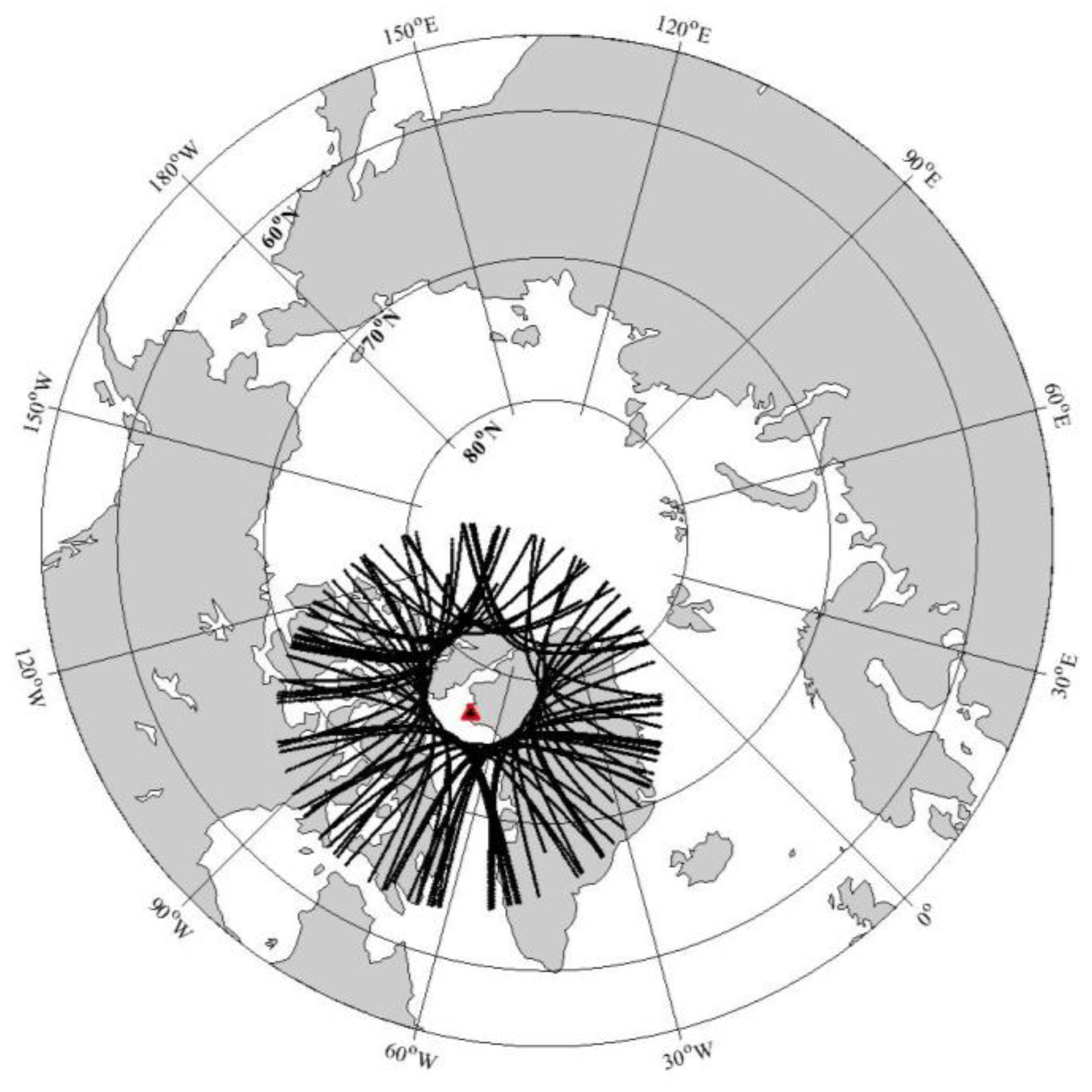
Figure 2.
Comparison of two MVTEC time series calculated using different methods for the same data: The blue line represents data computed from 35 Greenlandic GNSS ground stations using Bernese 5.0 software, while the red line shows data derived from the Thule single-station GNSS receiver using JPL-GIM.
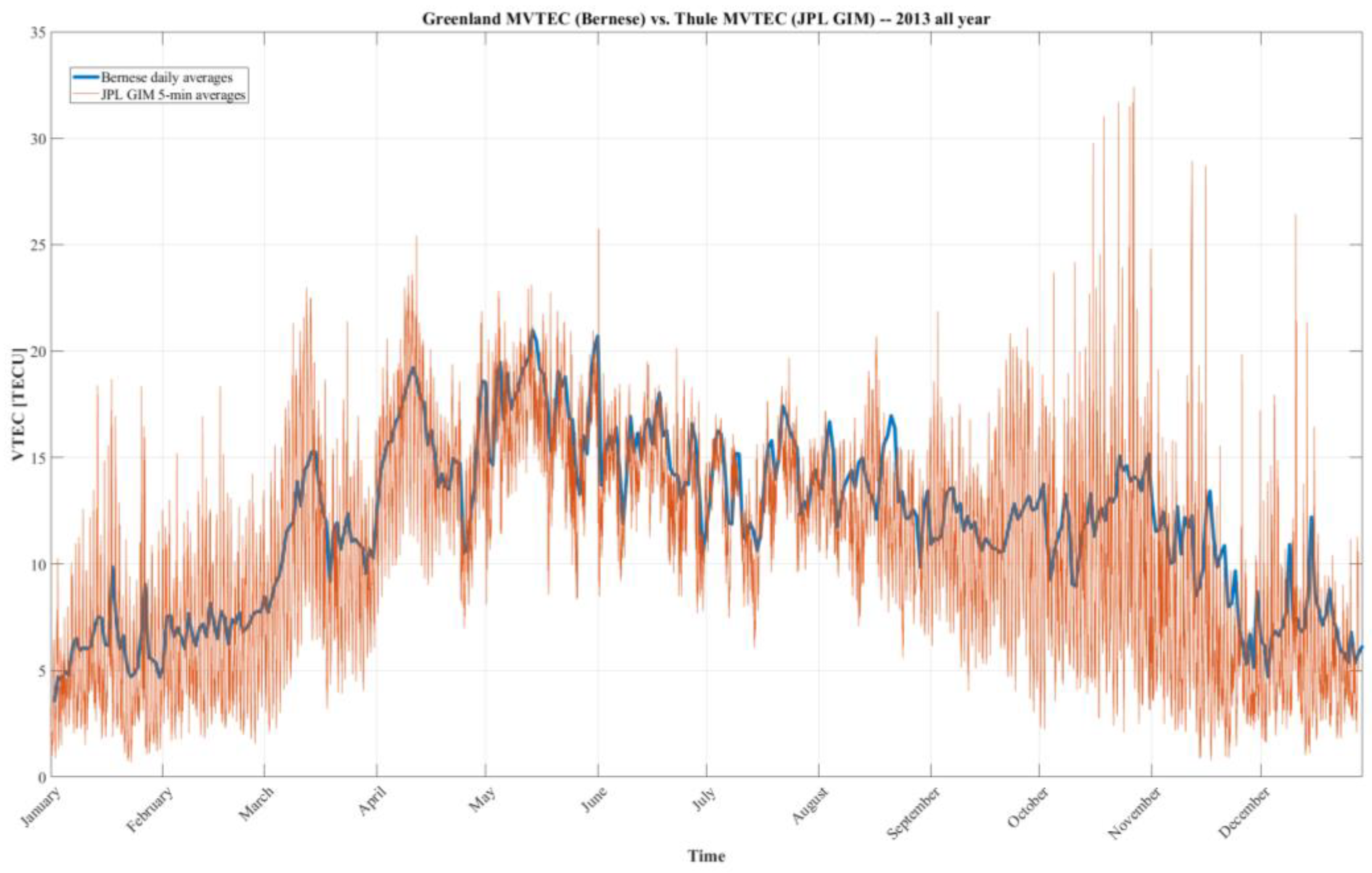
Figure 3.
This figure presents several data sets from 2013 and 2014: (a) MVTEC time series alongside OMNI-derived sunspot numbers, showing a strong correlation between sunspot numbers and the ~27-day TEC fluctuations. This correlation is especially evident during the summer months, when ionospheric variability, as reflected by MVTEC, is lower, reducing noise-like features. (b) The F10.7 index, used as a proxy for solar EUV radiation. (c) The PCN index, which represents solar wind energy input into the polar cap. (d) The AE index, and (e) the Dst index, both of which clearly highlight individual geomagnetic storms. However, neither index shows a significant influence on the TEC climatology at the timescale shown in this figure.
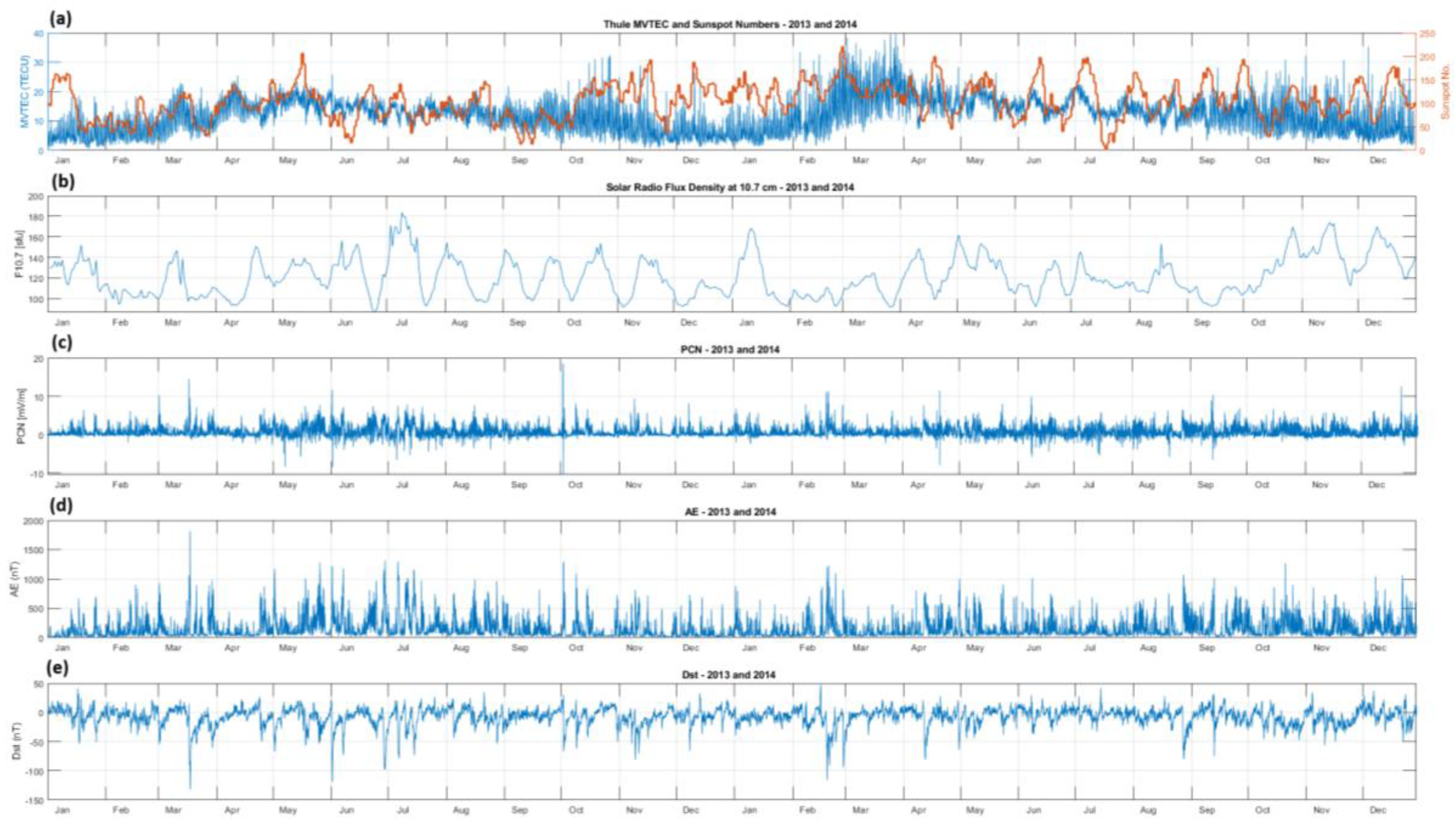
Figure 4.
The annotated MVTEC time-series and the PCN index are presented for the same set of months. (a) The MVTEC data can be distinguished by periods of high variability from fall to spring equinoxes, contrasted with the more stable summer months. (b) The PCN index exhibits greater fluctuations during the summer, when the northern polar cap faces the sun, and reduced variability in the winter months, with no noticeable increase in activity around the equinoxes.
Disclaimer/Publisher’s Note: The statements, opinions and data contained in all publications are solely those of the individual author(s) and contributor(s) and not of MDPI and/or the editor(s). MDPI and/or the editor(s) disclaim responsibility for any injury to people or property resulting from any ideas, methods, instructions or products referred to in the content. |
© 2024 by the authors. Licensee MDPI, Basel, Switzerland. This article is an open access article distributed under the terms and conditions of the Creative Commons Attribution (CC BY) license (https://creativecommons.org/licenses/by/4.0/).
Copyright: This open access article is published under a Creative Commons CC BY 4.0 license, which permit the free download, distribution, and reuse, provided that the author and preprint are cited in any reuse.


