Submitted:
17 October 2024
Posted:
18 October 2024
You are already at the latest version
Abstract
Welding spot defect detection using deep learning methods provides an effective way of body-in-white quality monitoring. Based on the existing Faster R-CNN model, this paper proposed an improved faster R-CNN model for resistance welding spot surface defect inspection to improve inspection efficiency and accuracy. The model contains the following improvements. Firstly, the improved algorithm uses anchor box with higher confidence output by the RPN network to locate welding spots. When a defect is detected and the detection system is in a suspended state, the Fast R-CNN network is used to confirm the defect category and details. Secondly, a new pruning model is proposed to replace the entire backbone neural network, which unnecessary convolutional layers and connection layers are deleted, and some parameters of each hidden layer are further reduced. On the premise of ensuring detection accuracy, the parameter quantity is extremely reduced, and the speed is improved. Experiments show that the model proposed in this paper took about 15ms for one single image test, and both the detection accuracy and recall rate reached over 90% according to the test on our dataset. This deep learning model meets the requirements of welding spot defect detection.
Keywords:
resistance spot welding
; surface defect detection
; deep learning model
; Faster R-CNN
; small object detection
1. Introduction
Welding spot quality is a very crucial factor that affects the hardware reliability of auto-body manufacturing. In body-in-white (BIW) production phase, the resistance spot welding (RSW) method is widely used. A lot of traditional image processing technics were adopted in some previous work [1]. However, these methods cannot work well with the influence of environmental factors such as vibration, dust, lightness, which all usually appear during the inspection [2]. Therefore, the manual visual inspection method is still used for surface defect inspection in lots of workshops nowadays.
At present, the quality inspection of BIW welds mainly includes two types of methods: non-visual method and visual inspection method [3]. And these methods can be divided into non-destructive testing technology and destructive testing technology. non-visual methods mainly include ultrasonic testing, X-ray inspection, dynamic resistance monitoring, tensile testing and electromagnetic testing [4].
Ultrasonic non-destructive testing (NDT) is widely applied in the evaluation of resistance spot welding detection. By emitting high-frequency sound waves and capturing their reflections, the detection is allowed to check internal defects such as cracks or porosity within welds. Mirmahdi et al. [5] provided a comprehensive review of ultrasonic testing for resistance spot welding, highlighting its effectiveness in determining the integrity of welding spots. Similarly, Yang et al. [6] explored the use of ultrasonic methods to assess weld quality, demonstrating its accuracy in identifying internal inconsistencies. Amiri et al. [7] used a neural network to study the relationship between the results of ultrasonic testing with tensile strength and fatigue life of spot welded joints.
X-ray imaging is another well-established NDT method used to examine the internal structure of spot welds. This technique creates radio-graphic images that allow for the identification of defects such as voids or incomplete fusion. Juengert et al. [8] employed X-ray technology to inspect automotive spot welds, showcasing its ability to reveal internal defects that may compromise weld strength. Similarly, Maeda et al. [9] investigated X-ray inspection of aluminum alloy welds, confirming its capability in the non-invasive evaluation of weld quality.
Dynamic resistance monitoring involves analyzing changes in welding current, voltage, and resistance during the welding process to infer weld quality. Butsykin et al. [10] explored the application of dynamic resistance in real-time quality evaluation of resistance spot welds, suggesting that fluctuations in resistance provide key indicators of weld formation. Wang [11] developed this approach, demonstrating its effectiveness in detecting weld faults through real-time monitoring of resistance signals.
Visual inspection, combined with the tapping method, is a simple yet widely-used approach for surface quality checks. By examining the weld for surface defects such as burns or inconsistencies, it provides initial insights into weld integrity. Dahmene [12] integrated visual inspection with acoustic emission to enhance defect detection in spot welding, illustrating the method's potential when combined with other techniques. Similarly, Hopkinson et al. applied acoustic testing to assess weld integrity, revealing a correlation between sound emissions and weld defects.
Tensile testing, a destructive evaluation method, is employed to measure the mechanical strength of spot welds by applying stress until failure occurs. Safari. [13] investigated the tensile-shear performance of spot welds, providing insights into the relationship between mechanical properties and weld quality. D.J. et al. [14] examined failure modes in tensile testing, offering detailed analysis on the impact of weld conditions on shear strength and failure behavior.
Electromagnetic testing is also a non-contact method that evaluates the electromagnetic properties of welds to detect imperfections. Tsukada et al. [15] utilized magnetic flux leakage testing to detect imperfections in automotive parts, affirming its role in efficient weld detection. They demonstrated the use of electromagnetic NDT for quality assessment in resistance spot welding, showing how variations in magnetic signals can indicate weld defects.
Since an automobile workshop can generate batches of standard data very quickly, an automatic spot welding vision inspection system based on deep learning is a suitable choice. Computer vision systems leverage high-resolution imaging and advanced image processing algorithms to inspect the external characteristics of welds, such as size, shape, and surface defects. Ye et al. [16] applied a system for the quality inspection of RSW, showcasing the potential of automated optical systems for large-scale manufacturing. Yang et al. [17] developed an automated visual inspection system that combines image processing with artificial intelligence to enhance spot weld assessment.
Due to the powerful perception, recognition, and classification capabilities of deep learning, target detection based on deep learning is now a hot research field, which can be divided into One stage and Two stage. Typical target detection algorithms are shown in Table 1.
Transformer models become more and more popular in computer vision domain, particularly in tasks such as surface defect detection. The attention mechanisms in Transformers allow them to capture global context and long-range dependencies across an image, which is critical for identifying subtle or dispersed surface defects. Recent studies have proposed using Vision Transformers (ViTs) to detect surface irregularities, benefiting from their ability to model both local and global features without the need for convolutions particularly effective for detecting complex surface patterns in materials. Vision Transformers were shown to outperform convolutional models on various visual recognition tasks, including defect detection on manufacturing surfaces, by using self-attention mechanisms to capture relationships between distant parts of the image.
YOLO is a real-time object detection model known for its speed and accuracy. In surface defect detection, YOLO's single-shot approach is particularly advantageous because it processes the entire image at once, making it highly efficient for real-time industrial applications. YOLO models have been adapted to detect surface defects in manufacturing industries, especially in steel or fabric inspection. The model detects defects by identifying them as "objects" and uses bounding boxes to localize anomalies in a single pass. Dai et al .[4] Proposed an improved YOLOv3 method with use of MobileNetV3.
The SSD model is another real-time object detection algorithm that excels in speed and accuracy, making it well-suited for surface defect detection in industrial settings. Like YOLO, SSD processes images in a single pass, but it uses multiple feature maps of different sizes to detect objects (or defects) at various scales. This feature makes it particularly effective for detecting defects that vary in size, such as small scratches or large dents on a surface. Li et al. [27] proposed an SSD based model to detect surface defects in ceramic materials, showing that the multi-scale feature extraction capability of SSD is beneficial for identifying both small and large-scale defects in real-time production environments.
The R-CNN family of models is widely applied for object detection and has been adapted for surface defect detection due to its robust performance in handling region proposals and localization. R-CNN models generate region proposals that likely contain defects, which are then classified and localized. Although slower than YOLO and SSD, R-CNNs are highly accurate and are often used in applications where detection precision is paramount. Wang et al. [28] applied Mask R-CNN to detect rail surface defects, demonstrating that despite the slower inference time, the model's high precision is advantageous for identifying critical defects that require exact localization.
SPPNet improves upon traditional CNNs by introducing spatial pyramid pooling, which allows the model to handle images of varying sizes without the need for resizing. This feature makes SPPNet particularly useful in surface defect detection tasks, where defects might appear at different scales across different products. The model’s ability to pool spatial information at multiple scales enhances its ability to detect both small and large surface defects. Quantity of studies employed SPPNet defects on the surface of metallic materials, finding that the multi-scale pooling allowed the model to capture details of both microscopic surface roughness and larger structural defects.
Faster R-CNN extends R-CNN by integrating a Region Proposal Network (RPN) that significantly accelerates the process of generating region proposals. Faster R-CNN combines the precision of R-CNN with greater computational efficiency, making it suitable for detecting defects in industrial applications where accuracy and speed are both critical. This model has been widely utilized in detecting surface cracks, scratches, and other anomalies in BIW. Luo et al. [29] developed an FPC surface defect method based on the Faster R-CNN object detection model, achieving high precision and recall while maintaining a reasonable inference speed, making it ideal for quality control in high-precision manufacturing.
In this paper, a lightweight deep learning detection model for small objects(RSW) is proposed to detect welding spots' position and quality. In order to increase the speed of model calculations, the Faster R-CNN algorithm uses a shared feature extraction layer structure, which greatly reduces the amount of parameters and simplifies calculations. The Faster R-CNN detection algorithm based on the VGG-16 [30] model has achieved 86.2% and 90.4% accuracy (mAP) on the PASCAL VOC 2007 and PASCAL VOC 2012 data sets, respectively, and the detection speed is 5 fps, which is a milestone in target detection. The algorithm is currently widely used in various target detection scenarios.
2. Proposed Approaches
2.1. Principle of Defect Detection Algorithm Based on Improved Faster R-CNN
The Faster R-CNN [25] detection algorithm is a two-stage high-efficiency target detection algorithm proposed by Yuming He and others in 2015, which has the advantages of fast speed and high accuracy. This algorithm first proposed the concept of region proposal network (RPN), using neural network to extract candidate detection regions, and based on candidate regions, using the target detection principle of Fast R-CNN [24] algorithm for target classification and target positioning.
The Faster R-CNN detection algorithm can be divided into three main parts: convolution feature sharing, RPN candidate region decision-making, target regression, and classification calculation. Its overall structure is shown in Figure 1.
Shared feature extraction layer: The feature extraction layer architecture of the Faster R-CNN algorithm is similar to other convolutional neural networks. It is a combination of a series of convolutional layers, pooling layers and ReLU activation layers. In the algorithm, the author performs feature extraction operations based on the two structures of VGG-16 and ZF respectively. The comparison between the two is shown in Table 2.
From the comparison of the above table, we can see that VGG-16 has more layers and a deeper network, so it is conducive to extracting more subtle features. However, the huge amount of parameters affects the calculation speed. Compared with ZF, the detection speed is greatly improved, and at the same time, it can guarantee a higher accuracy rate (62.1%). Therefore, the feature extraction layer based on the ZF structure is used in this article to satisfy real-time requirements for welding spot defect detection.
2.2.RPN Candidate Region Decision-Making
The feature map generated after extraction by the convolutional network ais input to the RPN network to generate a series of rectangular region candidate frames and scores. Different from the manual sliding window target area selection method based on the SS algorithm, RPN uses neural network to further extract the feature map features and generate anchor boxes of different scales (the number is k) at each point of the feature map, and map them to the original image, Carry out coordinate regression calculation and target judgment through neural network. At each feature point, RPN predicts 2k scores (probability of being/not the target), and 4k values (target coordinates). The detailed RPN structure is shown in Figure 2.
In order to adapt to different detection sizes, the anchor can change the size according to the actual detection situation, and adjust the ratio of width to height and zoom ratio. The size of the receptive field of the feature map is the basic size of the anchor setting. In the ZF model, after multi-convolutional layer down-sampling, the receptive field of the feature map is 16×16, so the anchor can be pulled on the basis of 16×16. Stretch or zoom. The size of the defect image detected in this article is 640×480. After the feature extraction of the convolutional layer, the feature map size is 50×37, then a total of 50×37×k anchor boxes are generated, and k is the number of anchor box types. The anchor box setting diagram is shown in Figure 3.
Figure 2.
RPN structure.
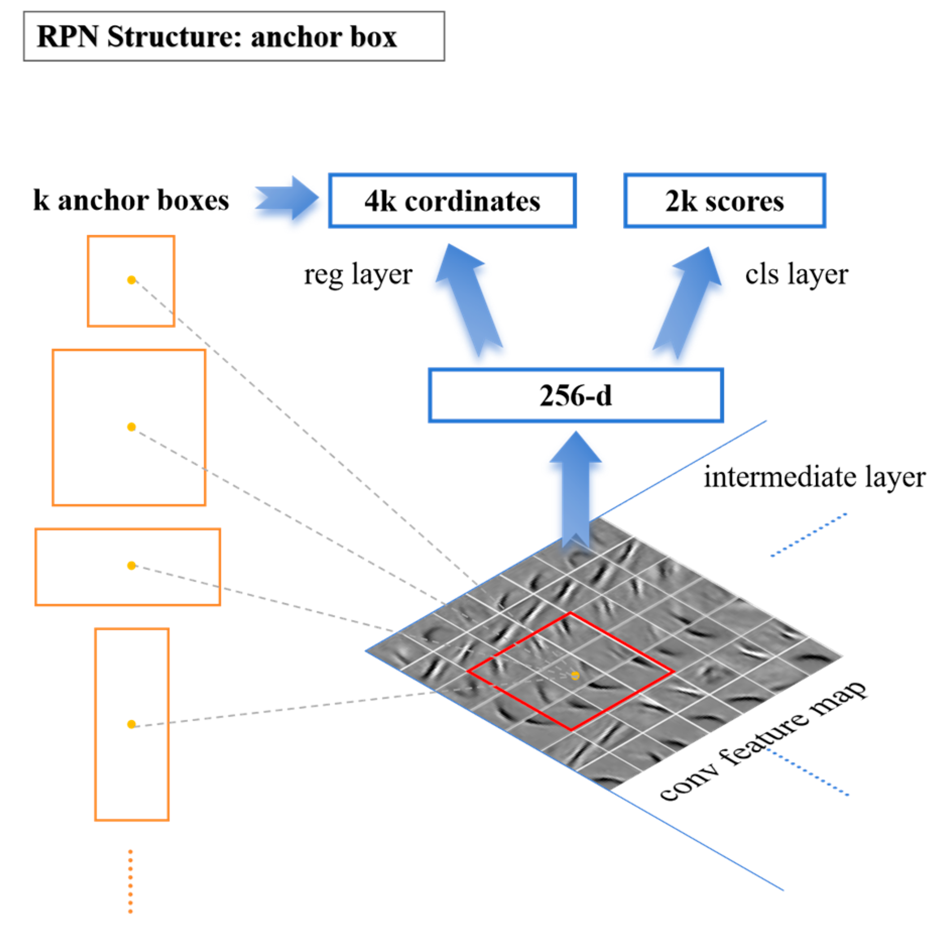
During training process, each anchor box may be close to the ground-truth box (the target marked in the training sample). We need to judge whether the anchor has a target based on the relationship between the anchor box and the adjacent ground truth box, so we adopt the method of calculating the intersection-over-union ratio IoU, as shown in Equation (1). Between the two, that is to measure the closeness between the anchor box and the ground-truth by the ratio of the overlapping area to the total area.
Mark the anchor according to the value of IoU, and decide whether the anchor participates in training. The marking method is expressed in Equation (2).
It can be seen from the above that the anchor box corresponding to the same ground-truth box, the IoU is the maximum value or the value is greater than 0.7 is a positive sample, the value is less than 0.3 is a negative sample, and the rest are not involved in the training, after preliminary marking and screening , Which greatly reduces the number of anchor box training, and only trains the samples that have an impact on the result. Random sampling is performed in batches in the marked anchor box samples during training process, and each batch of data ensures that the data of the positive sample and the data of the negative sample are 1:1.
For each prediction box, you need to perform category output and coordinate regression output. The category output can use the Softmax function to calculate the probability of belonging to the positive sample and the negative sample respectively. The coordinate regression output uses the feed-forward operation to obtain the coordinates of the prediction box, and calculate the The offset between the prediction box and the anchor box and the offset between the ground-truth box and the anchor box are optimized to minimize the difference between the two offsets. The offset between the two coordinates can be expressed as Equation (3):
:the center coordinates, width and height of the anchor box;
:the center coordinates, width and height of the ground-truth box.
During training, the joint optimization method of multi-task solving is adopted, and the loss function is composed of classification loss and regression loss. In this article, the positive and negative samples of the anchor box are marked as a multi-class problem, and the Softmax output unit is used, so the loss function based on negative logarithm is used together; the coordinate prediction of the anchor box is a regression problem, and the improved SmoothL1 loss function is used to calculate the prediction The distance between the coordinates and the true value. The loss function is expressed in Equation (4):
Fast R-CNN target detection calculation: First, the selected candidate frame is matched with the feature map extracted by the convolutional layer, and then the feature map is pooled with a fixed size, so that the feature map dimension when entering the fully connected layer is the same. At the end of the network, the Softmax output unit is also used to determine the specific types of defects, and the SmoothL1 loss function is used to correct the position of the defect to output more accurate position coordinates.
This article focuses on the common defects in actual production. According to statistics of existing defect samples, it is found that the largest defect is about 240 pixels *240 pixels, and the smallest defect is about 18 pixels *18 pixels. Therefore, the initial setting is 12 kinds of anchor box,. The ratio of width to height is [0.5,1,2] to cover the shape and size of the actual defect as much as possible. At this time k=12, when setting the convolution kernel dimension of RPN classification and regression output, it is also modified to cls: 2k=24, reg: 4k=48.
The network is split into two sub-networks respectively responsible for detecting defects and confirming defects. The RPN network is responsible for detecting whether there are defects, and the Fast RCNN network confirms the detailed information of the defects. The test network structure of the two sub-models is shown in Figure 4.
3. Experiments and Discussions
3.1. Dataset
In the welding industry, maintaining consistent resistance spot welding (RSW) quality relies heavily on stable process parameters. However, during real-world production, unexpected environmental factors such as fluctuations in electrode pressure, electrode wear, and contamination on the workpiece surface can disrupt the welding process. As a result, it becomes challenging to ensure the quality of every spot weld in high-volume, fast-paced automotive assembly lines. To address this, the paper introduces an image acquisition and quality inspection system aimed at detecting defective welds caused by such environmental disturbances. The system processes raw images captured on the assembly line, which contain significant environmental background noise. Figure 5. illustrates the workflow of the weld quality inspection process. The developed algorithm detects spot weld locations and isolates images of defective welds for further analysis.
To maintain safety standards, reduce maintenance costs, and prevent catastrophic failures, auto body assembly lines cannot tolerate faulty process parameters. As a result, collecting a substantial number of defective spot weld images, particularly rare defect types, becomes highly resource-intensive. In collaboration with automotive companies, thousands of spot welds are manually inspected, leading to the collection of a considerable dataset of defective spot weld images. The materials predominantly used in auto body assembly are zinc-coated steel sheets. Some typical defective spot welds, which are visually identifiable, are illustrated in Figure 5. The features of these defective welds are distinct, making them easier for deep learning models to recognize. The proposed algorithm focuses on detecting visually distinguishable defective spot welds.
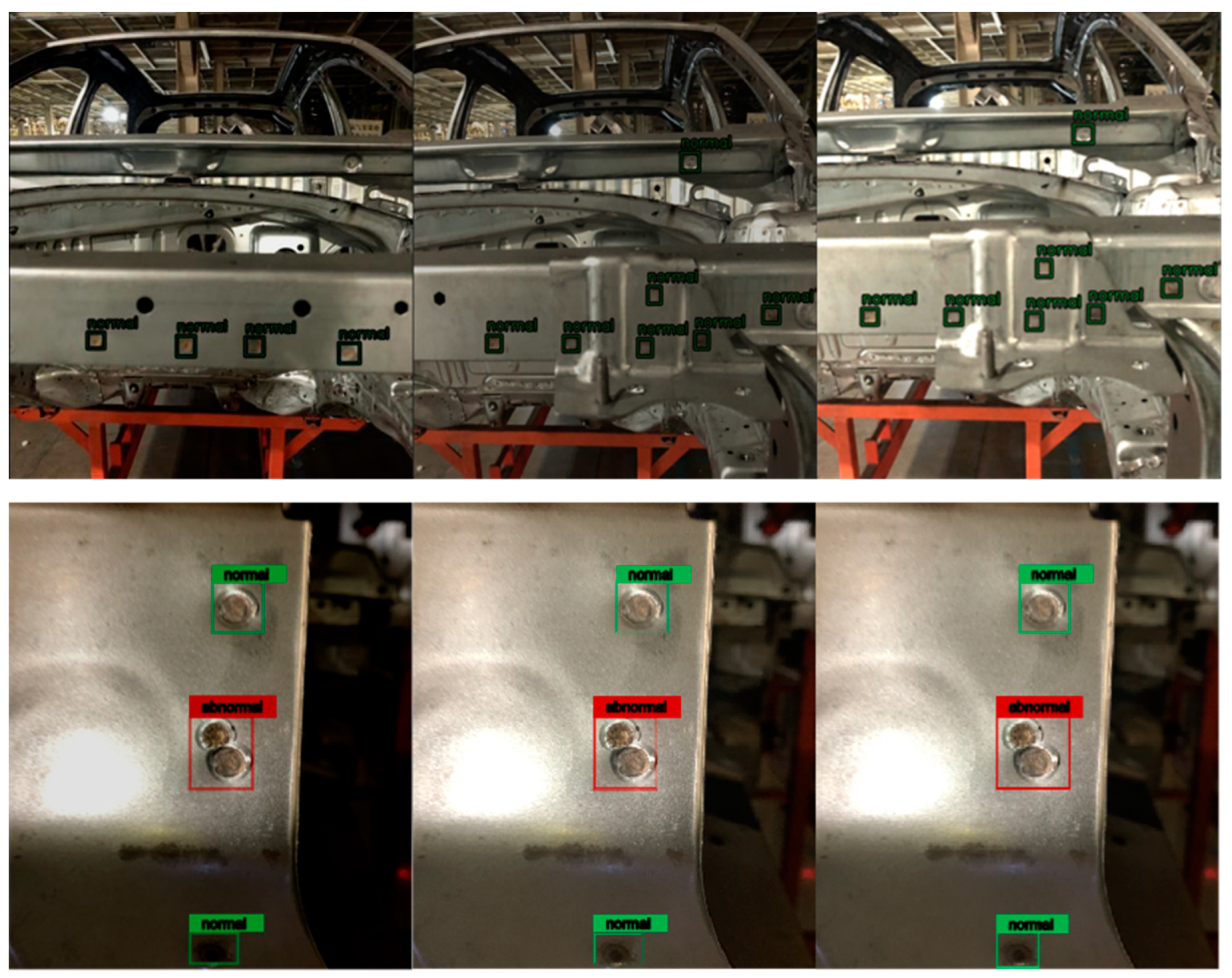
For the algorithm verification, the object detection model requires a well-labeled dataset. As no pre-existing dataset for auto body spot welds is available, 1,000 images of spot welds at various positions were collected from an automotive assembly line. The RSW quality vision inspection experimental platform is depicted in Figure 5. By varying the position of the robot arm, numerous spot welding images were captured using an RGB camera. Each image in the dataset has a resolution of 4032×3024 pixels, with some spot welds representing only one-thousandth of the total image, making them small targets. The spot welds were annotated to form a body welding spot detection dataset, consisting of 800 images for training and 200 for testing. An expert engineer annotated the spot welds and classified their quality as "normal" or "abnormal," which served as the ground truth. The defective spot welds were further categorized by defect type, such as crack, spatter, or undercut. Image samples of BIW welding spots and corresponding labels are displayed in Figure 6.
3.2. Experimental Results and Discussions
3.2.1 Pruning Optimization Experiment Results
The experiments were performed on a system equipped with an NVIDIA GeForce GTX 2080ti GPU, using the PyTorch deep learning framework for implementation. The input images used for training were resized to a resolution of 512×512 pixels. A total of 320 images were employed for data augmentation and model training. The model was trained for 500 epochs using the Adam optimizer [31], with an initial learning rate set to 0.001 for a batch size of 8. The learning rate was reduced by a factor of 10 whenever the validation loss plateaued. The model that achieved the best performance on the validation set during the training process was saved for further evaluation.The proposed model is compared with several typical object detection algorithms on the spot welding test set, such as SSD, Fast R-CNN, and CNN-Lenet5 [32].
Neural network parameters are numerous and require a lot of computing resources and memory, which makes it very difficult to deploy neural networks in embedded devices. As analyzed above, a large neural network may have more redundant parameters, and some connections between layers are not important. Removing these redundant parameters and connections can further optimize the model. In order to reduce the redundant parameters of the model, improve the detection speed, and facilitate the deployment of the neural network model in the actual production detection system, In this paper, combined with the visualization results of the output of each layer, pruning experiments on different scales of the model are carried out, and the structure and parameters of the model are optimized. The experiment content is shown in Table 3.
Analysis of pruning optimization experiment results:
1).It can be seen from experiments 1-4 that with the decrease of network parameters, the training time and testing time both decrease significantly. From the test results, the reduction of parameters will cause the fluctuation of test mAP (mean average precision). According to the analysis, there are two reasons for this phenomenon: one is to modify the entire network, and it is impossible to perform migration learning based on the pre-trained model, and the degree of model training is not enough; the other is to modify the model to a large extent, which damages the model. The detection capability. But in general, the modified models of different scales all have better detection performance, which shows that the algorithm has a certain degree of stability and robustness.
2).It can be seen from experiments 1-6-7 that the fully connected layer occupies most of the parameters of the entire network, and the pruning of the fully connected layer has an obvious effect on reducing the amount of parameters of the entire model. After pruning the fully connected layer, the model checking performance has improved significantly (mAP: 91.2%). Experiment 7 is carried out on the basis of Experiment 5 and Experiment 6, and the fourth convolutional layer and the fully connected layer are pruned at the same time. The experimental results show that the model parameters are reduced by about 50%, the amount of calculation is reduced, and the training of the model is greatly reduced. Time and detection time, and model detection performance has been further improved (mAP: 92.5%). The reason for the improved performance after analysis is: Because the training data set used by the model in this article is small and the data distribution is simple, it is easy to train with a more complex model. The phenomenon of over-fitting is caused by targeted reduction of network parameters, which reduces the non-linearity of the network, reduces the occurrence of over-fitting to a certain extent, and improves the detection performance of the model.
3.2.2. Comparison between the Proposed Model and Typical Model
A qualitative comparison between SSD, CNN-Lenet5, and the proposed model is conducted by visualizing images in Table 4 and Figure 7, where the predicted results are compared with ground truth labels. The findings indicate that deep learning models exhibit robustness in detecting the positions of appropriately sized spot welds while accurately assessing their quality. Additionally, the tested sample images contain multiple circular holes, which would likely be misidentified as spot welds if the traditional Circular Hough Transform algorithm [33] were applied. However, the deep learning model effectively addresses this limitation. Compared to the other models, the proposed approach provides the most accurate results in alignment with the ground truth.
These results highlight the proposed model’s capability in predicting spot welds of varying sizes, including smaller welds that are often missed during manual inspection. To further test the model’s generalization ability, some spot welds in the training set were deliberately left unlabeled. When the trained model was applied to these samples, it successfully identified the previously overlooked spot welds, as demonstrated in Figure 8, confirming the strong generalization performance of the model.

Table 4.
Comparison between the proposed model and typical models.
| Model | mAP | Time/s |
|---|---|---|
| SSD | 79.13% | 0.727 |
| CNN-Lenet5 | 84.69% | 0.837 |
| The proposed model | 92.50% | 0.969 |
Figure 7 shows sample results to verify the generalization ability of the models. CNN-Lenet5(left), the proposed model (middle) and the ground truth(right). The bounding box represents the good spot welds detected from the image, while red ones denote the bad spot welds. It can be found that the proposed model can recognize the good and bad welding spots well.
Figure 8.
Sample results to verify the generalization ability of the models. CNN-Lenet5(left), the proposed model (middle) and the ground truth(right).
Figure 8.
Sample results to verify the generalization ability of the models. CNN-Lenet5(left), the proposed model (middle) and the ground truth(right).
4. Conclusions
1).Novelty
This paper aims to predict the welding spot defects during the production of body-in-white by constructing a inspection system using an improved faster R-CNN model. This deep learning network model shows good performance on surface quality inspection for small object detection.
The improved algorithm uses the anchor box with higher confidence output by the RPN network to locate defects. When a defect is detected and the detection system is in a suspended state, the Fast R-CNN network is used to confirm the defect category and details. During training, the end-to-end training method is used to train the RPN network and Fast R-CNN network as a whole to ensure the stability of the network.
The threshold of IoU is increased to improve convergence speed and regression accuracy in the proposed model. The setting of the structure parameters in the network is more fit the characteristics of the welding spot surface defects, and the accuracy of the defect location is improved. Results on our dataset demonstrate that the proposed model has a better performance compared with several typical surface defect detection algorithms.
2).Limitation
Due to the actual environment of the production line, we are unable to collect more sufficient data sample. The number of samples in the dataset is insufficient and unbalanced, when the model is trained, it may cause a over-fitting phenomenon,which may miss detection and recognition errors in the real test.
3).Future work
The abundance of data plays a vital role in the performance of deep learning algorithms. In future work, it is necessary to improve the data management system, increase the number of samples, and improve the quality of samples. We hope to make some progress in the aspect of novel data augmentation.
Faster R-CNN, while accurate, is still slower than models like YOLO or SSD when used in real-time production environments. Future developments could focus on optimizing the Region Proposal Network (RPN) or incorporating lightweight architectures like MobileNet or EfficientNet into the Faster R-CNN pipeline to reduce inference time while maintaining accuracy.
Surface defects in weld spots often vary in size, from small cracks to large spatters. Faster R-CNN already handles multi-scale detection to some degree, but enhancing this capability and potentially through multi-scale feature extraction techniques like Feature Pyramid Networks (FPN), which could lead to even better detection of tiny or barely visible defects.
Author Contributions
Conceptualization, W.L. and J.H.; methodology, W.L.; data collection, W.L., J,Q., and L.H.; writing—original draft preparation, W.L.; writing— review and editing, J.Q.; supervision, W.L.; validation, W.L.; funding acquisition, L.H. All authors have read and agreed to the published version of the manuscript.
Funding
This research is supported by National Natural Science Foundation of China (U23B20102, 52035007), Ministry of Education "Human Factors and Ergonomics" University Industry Collaborative Education Project (No.202209LH16).
Institutional Review Board Statement
Not applicable.
Informed Consent Statement
Not applicable.
Data Availability Statement
Open-sourse database of surface defect detection for testing the algorithm: Datasets for your research: MVTec Software;Weakly Supervised Learning for Industrial Optical Inspection | Heidelberg Collaboratory for Image Processing (HCI) (uni-heidelberg.de);GitHub - abin24/Magnetic-tile-defect-datasets.: dataset of the upcoming paper "Saliency of magnetic tile surface defects"; For the private RSW in BIW datasets, requests for access can be directed to weijie.liu@sjtu.edu.cn.
Acknowledgments
We would like to thank Hongpeng Cao for his insightful discussion and feedback in technical details.
Conflicts of Interest
The authors declare that they have no known competing financial interests or personal relationships that could have appeared to influence the work reported in this paper. The authors declare no conflicts of interest. The funders had no role in the design of the study; in the collection, analyses, or interpretation of data; in the writing of the manuscript; or in the decision to publish the results.
References
- Zhou, K.; Yao, P. Overview of recent advances of process analysis and quality control in resistance spot welding. Mech. Syst. Signal Process. 2019, 124, 170–198. [Google Scholar] [CrossRef]
- Wang, J.; Zhang, Z.; Bai, Z.; Zhang, S.; Qin, R.; Huang, J.; Wen, G. On-line defect recognition of MIG lap welding for stainless steel sheet based on weld image and CMT voltage: Feature fusion and attention weights visualization. J. Manuf. Process. 2023, 108, 430–444. [Google Scholar] [CrossRef]
- Hong, Y.; He, X.; Xu, J.; Yuan, R.; Lin, K.; Chang, B.; Du, D. AF-FTTSnet: An end-to-end two-stream convolutional neural network for online quality monitoring of robotic welding. J. Manuf. Syst. 2024, 74, 422–434. [Google Scholar] [CrossRef]
- Dai, W.; Li, D.; Tang, D.; Jiang, Q.; Wang, D.; Wang, H.; Peng, Y. Deep learning assisted vision inspection of resistance spot welds. J. Manuf. Process. 2020, 62, 262–274. [Google Scholar] [CrossRef]
- ‘A Review of Ultrasonic Testing Applications in Spot Welding: Defect Evaluation in Experimental and Simulation Results | Transactions of the Indian Institute of Metals’. Accessed: Oct. 17, 2024. [Online]. Available: https://link.springer.com/article/10.1007/s12666-022-02738-8.
- Ultrasonic Non-Destructive Testing and Evaluation of Stainless-Steel Resistance Spot Welding Based on Spiral C-Scan Technique’. Accessed: Oct. 17, 2024. [Online]. Available: https://www.mdpi.com/1424-8220/24/15/4771.
- Amiri, N.; Farrahi, G.; Kashyzadeh, K.R.; Chizari, M. Applications of ultrasonic testing and machine learning methods to predict the static & fatigue behavior of spot-welded joints. J. Manuf. Process. 2020, 52, 26–34. [Google Scholar] [CrossRef]
- Nondestructive Testing of Welds | SpringerLink’. Accessed: Oct. 17, 2024. [Online]. Available: https://link.springer.com/referenceworkentry/10.1007/978-3-030-73206-6_2.
- ‘Investigating delayed cracking behaviour in laser welds of high strength steel sheets using an X-ray transmission in-situ observation system: Science and Technology of Welding and Joining: Vol 25, No 5’. Accessed: Oct. 17, 2024. [Online]. Available: https://www.tandfonline.com/doi/abs/10.1080/13621718.2020.1714873.
- ‘Evaluation of the reliability of resistance spot welding control via on-line monitoring of dynamic resistance | Journal of Intelligent Manufacturing’. Accessed: Oct. 17, 2024. [Online]. Available: https://link.springer.com/article/10.1007/s10845-022-01987-0.
- A new measurement method for the dynamic resistance signal during the resistance spot welding process - IOPscience’. Accessed: Oct. 17, 2024. [Online]. Available: https://iopscience.iop.org/article/10.1088/0957-0233/27/9/095009/meta.
- Dahmene, F.; Yaacoubi, S.; El Mountassir, M.; Bouzenad, A.E.; Rabaey, P.; Masmoudi, M.; Nennig, P.; Dupuy, T.; Benlatreche, Y.; Taram, A. On the nondestructive testing and monitoring of cracks in resistance spot welds: recent gained experience. Weld. World 2022, 66, 629–641. [Google Scholar] [CrossRef]
- Safari, M.; Mostaan, H.; Kh, H.Y.; Asgari, D. Effects of process parameters on tensile-shear strength and failure mode of resistance spot welds of AISI 201 stainless steel. Int. J. Adv. Manuf. Technol. 2016, 89, 1853–1863. [Google Scholar] [CrossRef]
- D. J. Radakovic and M. Tumuluru, ‘Predicting Resistance Spot Weld Failure Modes in Shear Tension Tests of Advanced High-Strength Automotive Steels’.
- Tsukada, K.; Miyake, K.; Harada, D.; Sakai, K.; Kiwa, T. Magnetic Nondestructive Test for Resistance Spot Welds Using Magnetic Flux Penetration and Eddy Current Methods. J. Nondestruct. Evaluation 2013, 32, 286–293. [Google Scholar] [CrossRef]
- Ye, S.; Guo, Z.; Zheng, P.; Wang, L.; Lin, C. A Vision Inspection System for the Defects of Resistance Spot Welding Based on Neural Network. In Computer Vision Systems. ICVS 2017. Lecture Notes in Computer Science; Springer: Cham, Swizerland, 2017; Volume 10528, pp. 161–168. [Google Scholar] [CrossRef]
- Yang, Y.; Zheng, P.; He, H.; Zheng, T.; Wang, L.; He, S. An Evaluation Method of Acceptable and Failed Spot Welding Products Based on Image Classification with Transfer Learning Technique. In Proceedings of the 2nd International Conference on Computer Science and Application Engineering (CSAE2018), Hohhot, China, 22–24 October 2018; p. 109. [Google Scholar] [CrossRef]
- M. Jaderberg, K. Simonyan, A. Zisserman, and koray kavukcuoglu, ‘Spatial Transformer Networks’, in Advances in Neural Information Processing Systems, Curran Associates, Inc., 2015. Accessed: Oct. 17, 2024. [Online]. Available: https://proceedings.neurips.cc/paper_files/paper/2015/hash/33ceb07bf4eeb3da587e268d663aba1a-Abstract.html.
- J. Redmon, S. Divvala, R. Girshick, and A. Farhadi, ‘You Only Look Once: Unified, Real-Time Object Detection’. arXiv, May 09, 2016. [CrossRef]
- ‘[1512.02325] SSD: Single Shot MultiBox Detector’. Accessed: Oct. 17, 2024. [Online]. Available: https://arxiv.org/abs/1512.02325.
- Lin, T.Y.; Goyal, P.; Girshick, R.; He, K.; Dollar, P. Focal loss for dense object detection. IEEE Trans. Pattern Anal. Mach. Intell. 2020, 42, 318–327. [Google Scholar] [CrossRef]
- Girshick, R.; Donahue, J.; Darrell, T.; Malik, J. Rich Feature Hierarchies for Accurate Object Detection and Semantic Segmentation. In Proceedings of the IEEE Conference on Computer Vision and Pattern Recognition, Columbus, OH, USA, 23–28 June 2014; pp. 580–587. [Google Scholar] [CrossRef]
- He, K.; Zhang, X.; Ren, S.; Sun, J. Spatial pyramid pooling in deep convolutional networks for visual recognition. In European Conference on Computer Vision; Springer: Cham, Switzerland, 2014; Volume 8691, pp. 346–361. [Google Scholar]
- Girshick, R. Fast R-CNN. In Proceedings of the 2015 IEEE International Conference on Computer Vision (ICCV), Santiago, Chile, 7–13 December 2015; pp. 1440–1448. [Google Scholar] [CrossRef]
- Ren, S.; He, K.; Girshick, R.; Sun, J. Faster R-CNN: Towards real-time object detection with region proposal networks. IEEE Trans. Pattern Anal. Mach. Intell. 2017, 39, 1137–1149. [Google Scholar] [CrossRef] [PubMed]
- Lin, T.Y.; Dollár, P.; Girshick, R.; He, K.; Hariharan, B.; Belongie, S. Feature pyramid networks for object detection. In Proceedings of the IEEE Conference on Computer Vision and Pattern Recognition, Honolulu, HI, USA, 21–26 July 2017. [Google Scholar] [CrossRef]
- PDF) Research on a Surface Defect Detection Algorithm Based on MobileNet-SSD’, ResearchGate. Accessed: Oct. 17, 2024. [Online]. Available: https://www.researchgate.net/publication/327705107_Research_on_a_Surface_Defect_Detection_Algorithm_Based_on_MobileNet-SSD.
- Wang, H.; Li, M.; Wan, Z. Rail surface defect detection based on improved Mask R-CNN. Comput. Electr. Eng. 2022, 102. [Google Scholar] [CrossRef]
- Luo, W.; Luo, J.; Yang, Z. FPC surface defect detection based on improved Faster R-CNN with decoupled RPN. 2020 Chinese Automation Congress (CAC). LOCATION OF CONFERENCE, ChinaDATE OF CONFERENCE; pp. 7035–7039.
- K. Simonyan and A. Zisserman, ‘Very Deep Convolutional Networks for Large-Scale Image Recognition’. arXiv, Apr. 10, 2015. [CrossRef]
- Kingma, D.P.; Ba, J. Adam: A method for stochastic optimization. ArXiv 2014. [Google Scholar] [CrossRef]
- Lecun, Y.; Bottou, L.; Bengio, Y.; Haffner, P. Gradient-based learning applied to document recognition. Proc. IEEE 1998, 86, 2278–2324. [Google Scholar] [CrossRef]
- S. Hassanein, S. Mohammad, M. Sameer, and M. E. Ragab, ‘A Survey on Hough Transform, Theory, Techniques and Applications’. arXiv, Feb. 07, 2015. [CrossRef]
Figure 1.
Overall structure of the Faster R-CNN detection algorithm.
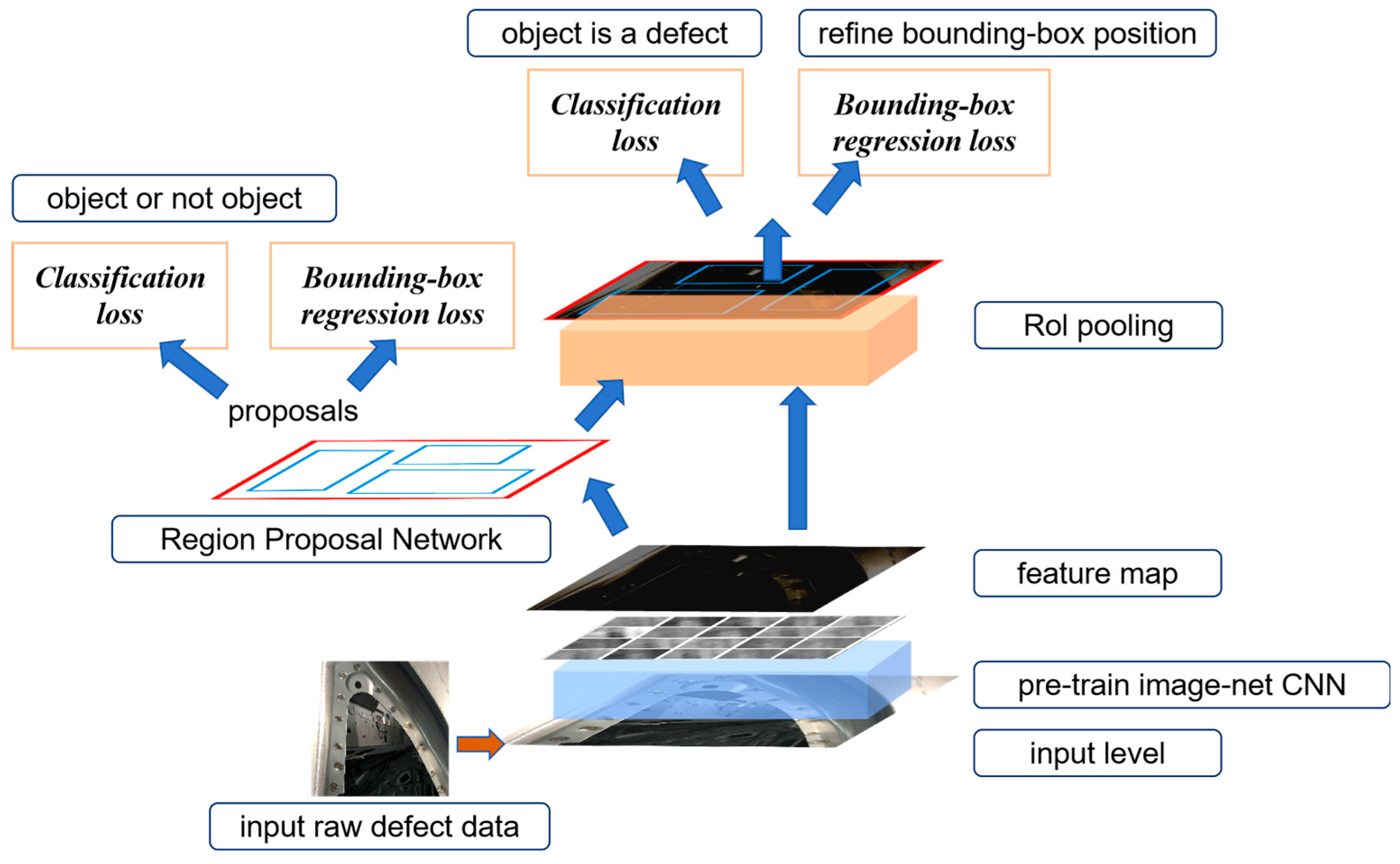
Figure 3.
anchor box setting diagram.
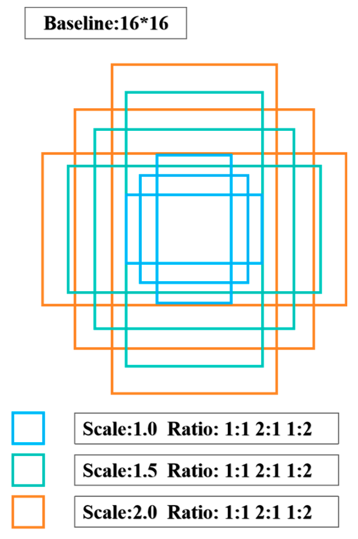
Figure 4.
Improved training network structure diagram. The RPN_forward structure(left), the Fast R-CNN structure(right).
Figure 4.
Improved training network structure diagram. The RPN_forward structure(left), the Fast R-CNN structure(right).
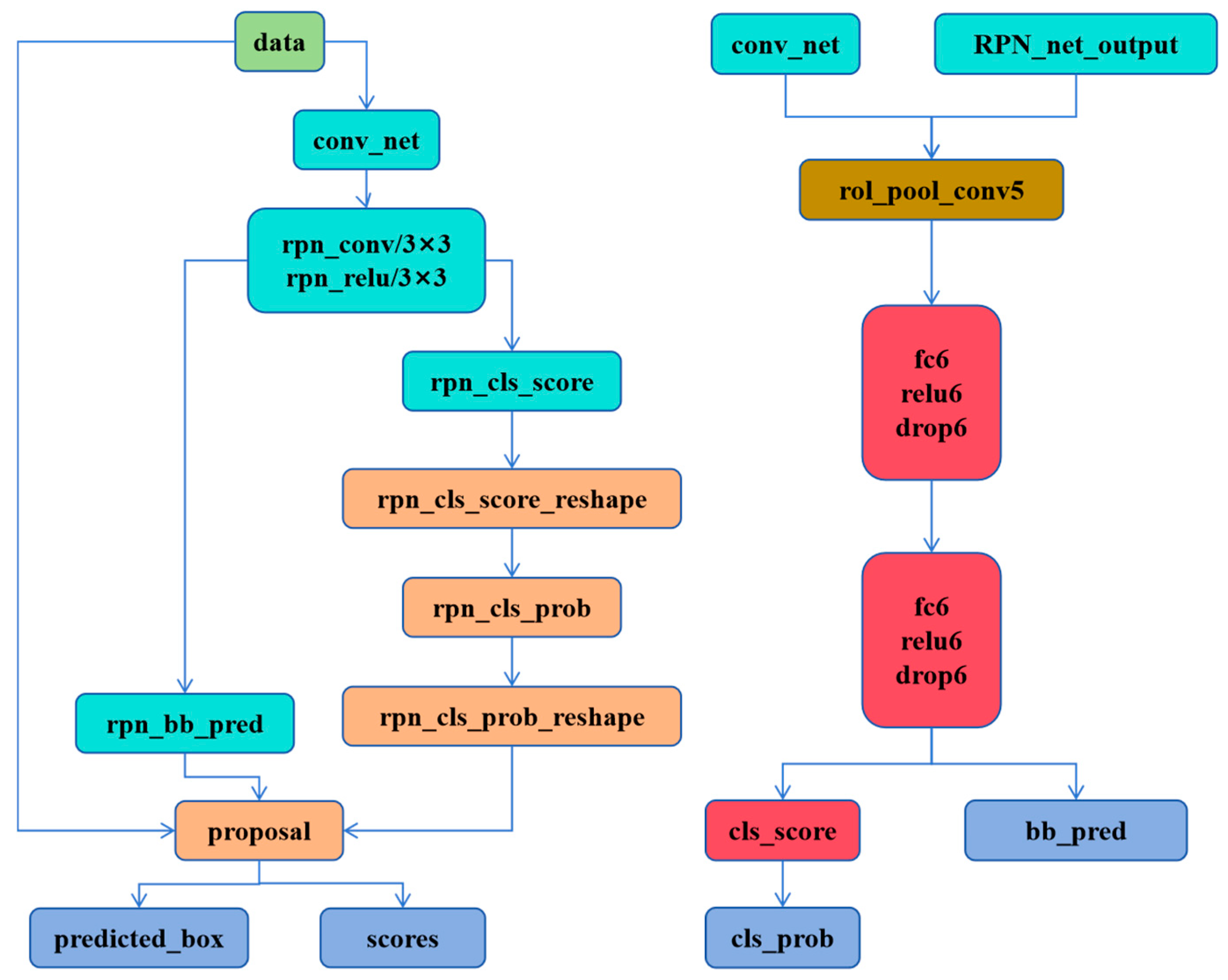
Figure 5.
The procedure diagram of the welding spot quality inspection process.
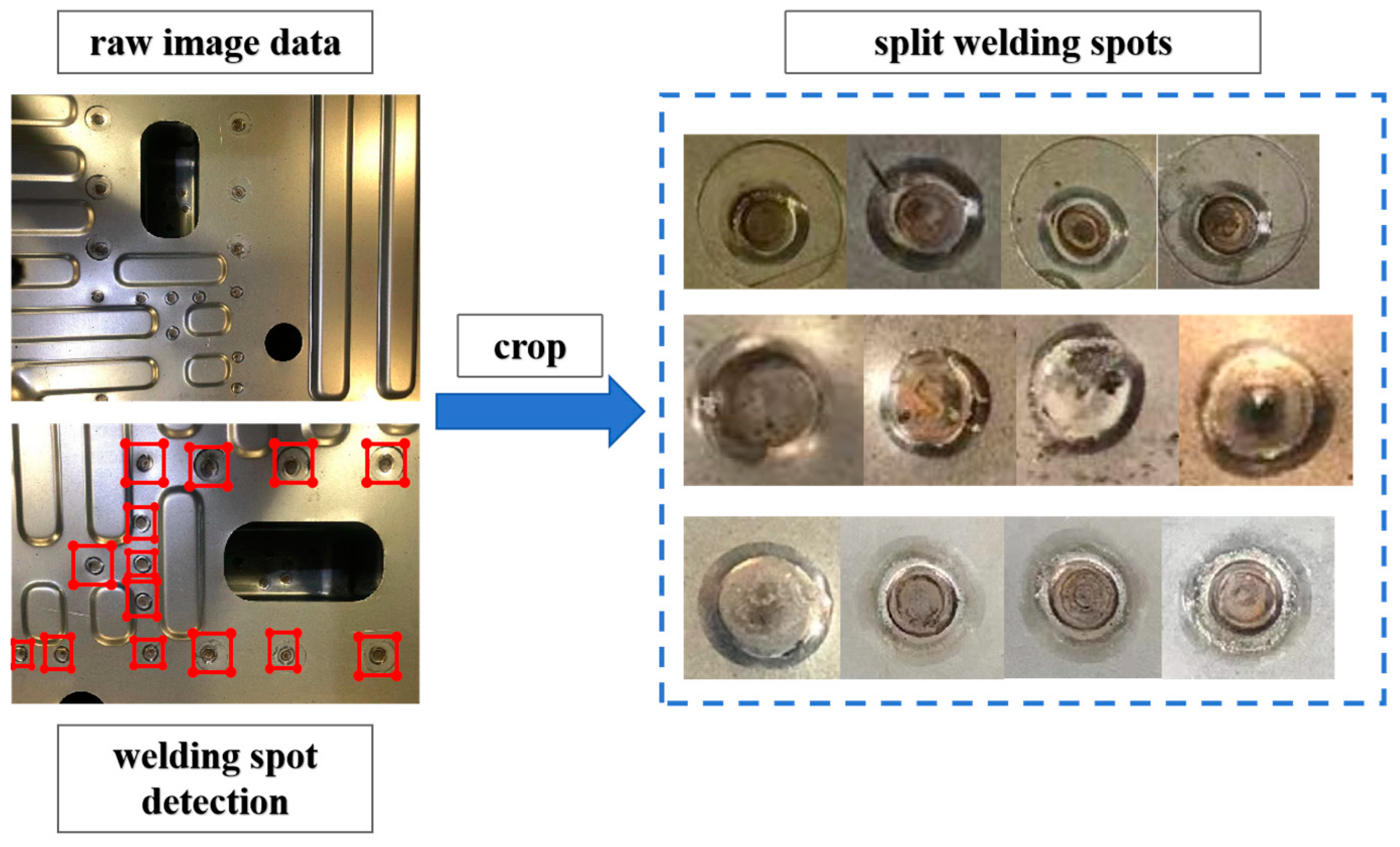
Figure 6.
Image samples of body-in-white welding spots and corresponding labels.
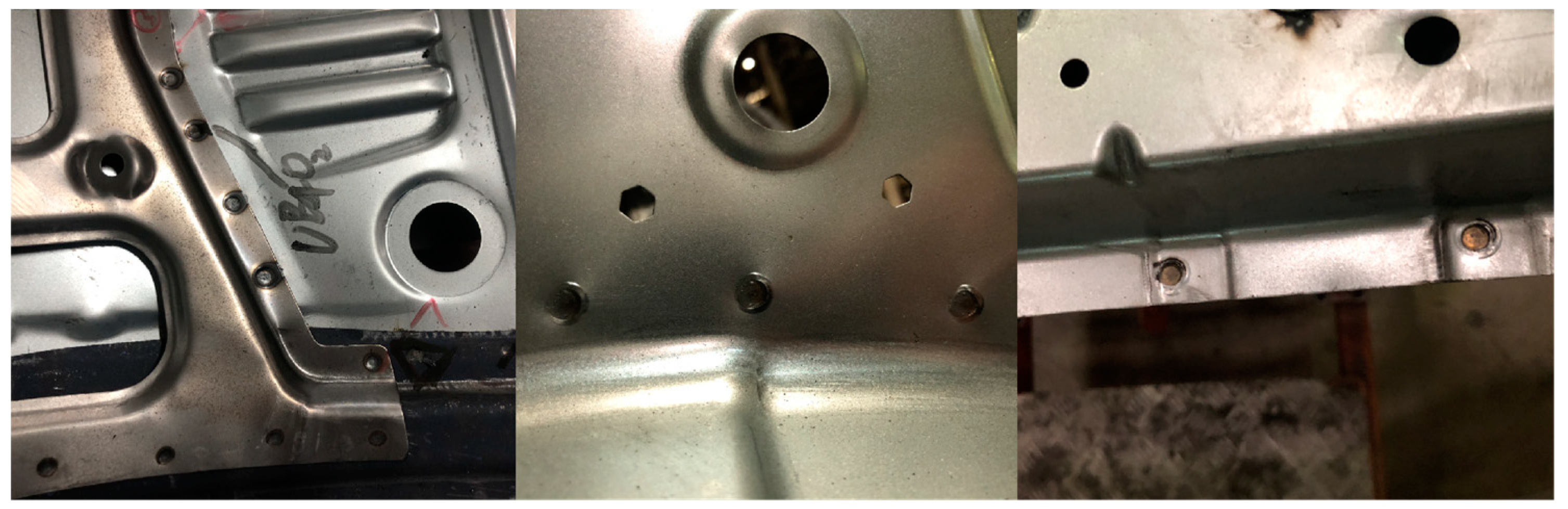
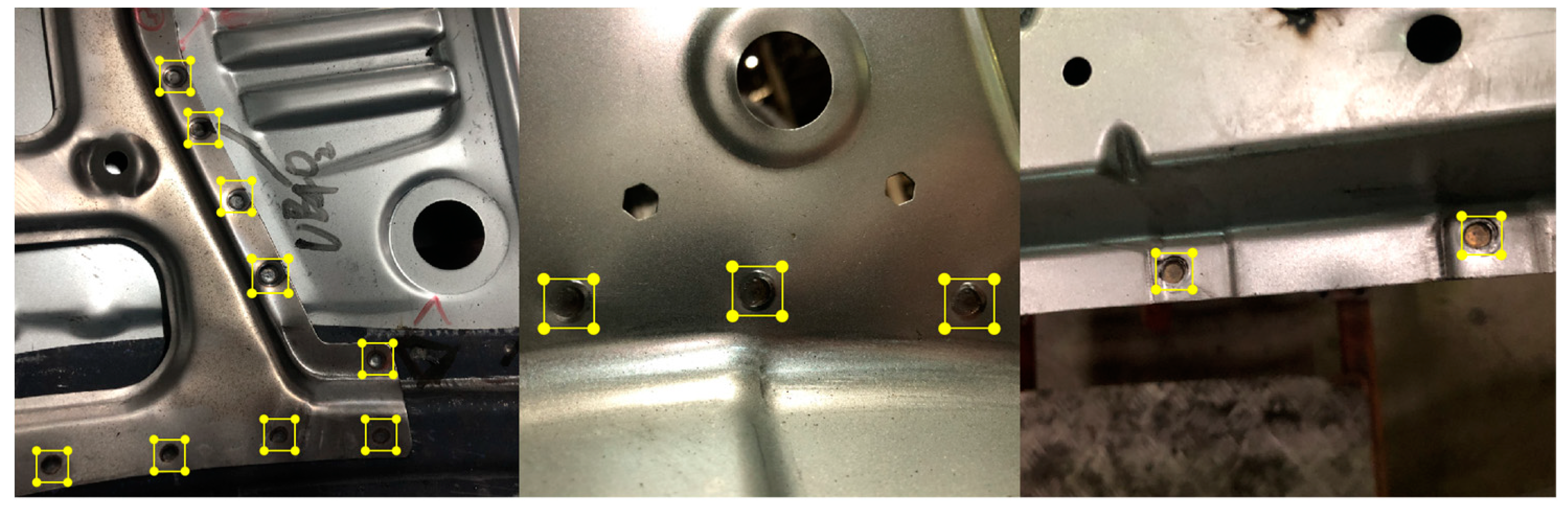
Table 1.
Typical target detection algorithms in deep learning
| Type | Algorithm |
|---|---|
| One stage | Transformer [18], YOLO [19], SSD [20], RetinaNet [21] |
| Two stage | R-CNN [22], SPPNet [23], Fast R-CNN [24], Faster R-CNN [25], FPN [26] |
Table 2.
Comparison of feature extraction layer structure based on VGG-16 and ZF.
| Name | CL | PL | AL | Parameter | mAP | fps |
|---|---|---|---|---|---|---|
| VGG-16 | 13 | 5 | ReLU | 14.7M | 73.2% | 5 |
| ZF | 5 | 2 | ReLU | 3.17M | 62.1% | 17 |
Table 3.
Model pruning optimization experiment.
| Number | Experiment | Parameter | Ts/frame | Ps/frame | mAP |
|---|---|---|---|---|---|
| 1 | Faster R-CNN | 57.8M | 0.043 | 0.031 | 89.8% |
| 2 | 1/2 Network-wide pruning | 14.6M | 0.021 | 0.008 | 88.7% |
| 3 | 1/4 Network-wide pruning | 3.7M | 0.008 | 0.004 | 86.5% |
| 4 | 1/8 Network-wide pruning | 0.9M | 0.005 | 0.002 | 85.1% |
| 5 | Delete the 4th Conv Layer | 56.5M | 0.041 | 0.030 | 90.7% |
| 6 | 1/2 connected layer pruning | 26.3M | 0.026 | 0.020 | 91.2% |
| 7 |
Delete the 4th ConvLayer and 1/2 connected layer pruning |
25.5M | 0.025 | 0.018 | 92.5% |
Disclaimer/Publisher’s Note: The statements, opinions and data contained in all publications are solely those of the individual author(s) and contributor(s) and not of MDPI and/or the editor(s). MDPI and/or the editor(s) disclaim responsibility for any injury to people or property resulting from any ideas, methods, instructions or products referred to in the content. |
© 2024 by the authors. Licensee MDPI, Basel, Switzerland. This article is an open access article distributed under the terms and conditions of the Creative Commons Attribution (CC BY) license (https://creativecommons.org/licenses/by/4.0/).
Copyright: This open access article is published under a Creative Commons CC BY 4.0 license, which permit the free download, distribution, and reuse, provided that the author and preprint are cited in any reuse.


