Submitted:
15 October 2024
Posted:
17 October 2024
You are already at the latest version
Abstract
What is an observer? What is an observation? How do observations inform beliefs? What is the relationship between observers and physical objects in spacetime? These are central, and as yet unresolved, questions in the foundations of physics and consciousness science. We propose an answer taking consciousness as fundamental, resulting in a theory of conscious agents whose mutual interaction is governed by Markov chains. We describe observation via a new trace order on Markov chains. In this context, no observer is aloof: it must be an integral part of any system it observes. We find that the trace order forms a non-Boolean logic, mapping homomorphically to the “Lebesgue” logic” of probabilistic beliefs. We explore implications of conscious agent theory for the “hard problem” of consciousness, and propose a route to empirical tests using data from scattering experiments with subatomic particles.
Keywords:
consciousness
; observation
; positive geometries
; Markov chain
; trace chain
; partial order
; Lebesgue order
; trace order
; scattering amplitudes
; decorated permutations
“Why may not the world be a sort of republican banquet of this sort, where all the qualities of being respect one another’s personal sacredness, yet sit at the common table of space and time? To me this view seems deeply probable. Things cohere, but the act of cohesion itself implies but few conditions, and leaves the rest of their qualifications indeterminate. ... if we stipulate only a partial community of partially independent powers, we see perfectly why no one part controls the whole view, but each detail must come and be actually given, before, in any special sense, it can be said to be determined at all. This is the moral view, the view that gives to other powers the same freedom it would have itself.”
William James, 1882 [1]
1. Introduction
Science weaves insights and observations, theories and experiments. When Galileo focused a telescope on Jupiter, its orbiting moons dethroned geocentrism, and demanded new theories.
What is an observer? What is an observation? How do observations inform theories?
Classical physics posits an observer that is distinct from, and need not disturb, what it observes. This observer can be safely ignored.
Einstein’s theories of relativity do not ignore the observer. But they identify it with a frame of reference—a system of coordinates and clocks.
In quantum theory the observer is essential, but ill understood. If a physical system is not observed, its state evolves according to Schrödinger’s equation, which is unitary and deterministic. But when the system is observed, its state “collapses”: a complex superposition of eigenstates becomes a single eigenstate. This collapse is nonunitary and random, and that is a problem: observation, being nonunitary, can’t be explained by quantum processes that are unitary. This is a remarkable failure of reductive explanation within quantum theory.
Some attempt to remedy this through the process of decoherence, in which a complex superposition of eigenstates evolves into a real mixture of eigenstates. But it does not evolve into a single eigenstate, and thus fails to model the collapse induced by observation.
Some propose to replace the term “observer” with “measuring apparatus,” which sounds less subjective. Werner Heisenberg, for instance, wrote, “Of course the introduction of the observer must not be misunderstood to imply that some kind of subjective features are to be brought into the description of nature. The observer has, rather, only the function of registering decisions, i.e., processes in space and time, and it does not matter whether the observer is an apparatus or a human being; but the registration, i.e., the transition from the “possible” to the “actual,” is absolutely necessary here and cannot be omitted from the interpretation of quantum theory” [3].
And Asher Peres wrote that observers in quantum physics are “similar to the ubiquitous “observers” who send and receive light signals in special relativity. Obviously, this terminology does not imply the actual presence of human beings. These fictitious physicists may as well be inanimate automata that can perform all the required tasks, if suitably programmed” [2].
This fails to resolve the issue. A measuring apparatus, even if not subjective, must still instantiate a nonlinear collapse, and nonlinearity is the stubborn problem that precludes a reductive account of measurement in quantum theory.
So quantum theory acknowledges the essential role of the observer, but offers no reductive theory of the observer. This has long been a source of consternation. As Frank Wilczek put it in 2006, “The relevant literature is famously contentious and obscure. I believe it will remain so until someone constructs, within the formalism of quantum mechanics, an “observer,” that is, a model entity whose states correspond to a recognizable caricature of conscious awareness … That is a formidable project, extending well-beyond what is conventionally considered physics.”
It is indeed formidable. This measurement problem prompted John Wheeler to suggest a complete rethinking of quantum theory: “It is difficult to escape asking a challenging question. Is the entirety of existence, rather than being built on particles or fields of force or multidimensional geometry, built upon billions upon billions of elementary quantum phenomena, those elementary acts of “observer-participancy,” those most ethereal of all the entities that have been forced upon us by the progress of science?” [24].
Wheeler’s challenge was accepted by his student Chris Fuchs, who developed QBism, an interpretation of quantum theory that promotes observing agents to the limelight [16]. In QBism, quantum states describe beliefs of agents, not their external reality as it is. If an agent says “this system has state ” she asserts nothing about that reality. She means that describes her probabilities for measurement outcomes. When she measures, she updates her belief, from to an eigenstate of the outcome. This “collapse” is no mystery. It is revising belief in light of new data.
What is an observing agent? QBism offers no theory. It simply says that, whatever an observer is, quantum theory describes its beliefs.
Thus Wilczek’s formidable project of modeling the observer remains unfinished. Wilczek reiterated its importance in 2022: “Quantum mechanics has an unusual mechanism since the theory has equations, and to interpret the equations one must make an observation. I believe that, eventually, in order to … fully understand quantum mechanics, we will need to understand that we have that model of consciousness that corresponds to our experience of everyday life, which is fully based on quantum mechanics. At present, I don’t think we have that” [12].
What we have, instead, is remarkable. In the last decade, theorists in high-energy physics have discovered geometric structures, entirely beyond spacetime and quantum theory, called “positive geometries.” These structures dramatically simplify the computation of particle interactions in spacetime, and reveal new insights about these interactions.
This success prompted the European Research Council to fund UNIVERSE+, an international collaboration of researchers that “seeks a new foundation for fundamental physics, ranging from elementary particles to the Big Bang, revealing a hidden world of ideas beyond quantum mechanics and spacetime. Novel geometric objects recently discovered in theoretical physics hint at new mathematical structures. Combinatorics, algebra, and geometry have been connected to particle physics and cosmology in an entirely unexpected way. Leveraging these advances, the team will launch the field of Positive Geometry, as a new mathematical framework for describing the laws of physics” [25].
Incredible. In the last decade, physics has taken its first peak beyond spacetime. And what does it see? Objects with positive geometries. This is ground breaking and exhilarating. It’s also puzzling. Why these objects and geometries? Why no dynamical systems? Why no observers? Who ordered this?
Positive geometries confound us, much as the obelisk in 2001: A Space Odyssey confounded the apes that swarmed it, hooting and pounding without comprehension. Positive geometries feel deep and important, but their deeper meaning eludes us.
Here we propose a deeper meaning. We propose that beyond positive geometries there lies a rich dynamics of “observer-participancy," just as Wheeler suggested. We model it as a dynamics of entities we call conscious agents (CAs). Positive geometries, we propose, describe the asymptotic behavior of CAs.
We briefly review CA theory (CAT) and the formulation of their experience dynamics as Markov kernels. We then introduce a partial order on Markov kernels: if M is a trace of N. Intuitively, M is a trace of N if M describes what you see when you watch the dynamics of N only on that subset of states: : we say that M is supported on that subset of the states.
The trace order, interpreted as logical implication, induces a logic, the trace logic, on the set of all Markov kernels. The trace logic is non-Boolean: it has no greatest kernel and many incomparable kernels. But the trace logic is locally Boolean: for a given N, the set of all M such that forms a Boolean logic.
The trace logic defines a theory of observation. Conscious agent Aobserves conscious agent B iff in the trace logic, where , respectively , is the “experience kernel” of A, respectively B. We express this by saying “”, and call this relation on CAs the “trace order” too. The relation “” is thus a preorder on the set of all CAs: two CAs with the same experience kernel Q will be indistinguishable in trace order. To simplify notation, we will henceforth use the same symbol, A, both for the CA A and for its experience kernel . This definition of trace order is the foundation of the trace theory of observation, and implies that any observer is an integral part of what it observes. Observers are not aloof, objective, and negligible. They are not just a system of coordinates and clocks. They are organically entwined with what they observe. This is a radical departure from standard notions of detached observers with paltry influence.
The trace theory of observation is, as we shall see, an ideal theory: the trace of a kernel demands an infinite sample of its dynamics. We assume that, as with our phenomenal experience, observation occurs via finite sampling of the observed. So we discuss finite sampling of trace chains, and their application to real experiments.
What does the CA A “observe” in a CA B, when the support of A is contained in the state space of B? We posit that A observes what it can of the long-term, or asymptotic dynamics of B. In fact, we show that if B is ergodic then A sees the asymptotic probabilities of states it shares with B. We quantify this using stationary measures. The stationary measure of a kernel P is a probability measure on the states of P satisfying ; describes the long-term probability that the dynamics of P will visit each of its states. We show that the stationary measure of A is the normalized restriction of the stationary measure of B. Thus A “sees” a probability measure that encodes long-term behaviors of B.
So observers are modeled as kernels, and observations yield probability measures. These probability measures express that which the observer can know about the observed: as in QBism’s approach, we take these probabilities to express the beliefs of the observer caused by observation. The set of all probability measures also has a logic, the Lebesgue logic, [7] which too is non-Boolean: it has no greatest kernel and many incomparable kernels. But the Lebesgue logic is again “locally” Boolean: for a given , the set of all such that implies forms a Boolean logic. We show that the map from kernels to stationary measures, i.e., from observation to belief, is a homomorphism from the trace logic to the Lebesgue logic: the logic of observation and the logic of belief mesh perfectly.
We then discuss our progress on projecting the dynamics of CAs onto positive geometries and thence into spacetime. We propose specific correspondences between properties of CAs and properties of particles in spacetime, including mass, energy, momentum and spin. We outline the work that remains to complete the projection and to make predictions testable by scattering experiments with particles.
2. Conscious Agents
We develop the CAT formalism in prior papers [5,33,34]. To keep this paper self contained, we briefly review the motivations and definition of CAs.
A scientific theory asks us to grant certain assumptions. If we grant them, the theory promises in return to explain some phenomena of interest. William of Ockham counsels theory builders to keep assumptions to a minimum. That is sage advice. The bare minimum, however, is never zero. Each theory has assumptions. So no theory explains everything in its domain: no theory explains its assumptions.
One may propose a deeper theory, which explains assumptions of a prior theory. But the new theory has its own, unexplained, assumptions. And so on, forever. Thus science can offer no theory of everything, in the sense of a theory that explains its own assumptions. (This is distinct from what physicists term a "theory of everything," which is one that unifies the known four fundamental forces.)
Since no theory can be a theory of everything, it follows that every theory has a scope and limits. A good theory provides mathematically precise tools to explore its scope. A great theory provides tools to discover its own limits.
Quantum field theory, for instance, which unites quantum mechanics and Einstein’s theory of spacetime, has marvelous scope and application. It also informs us of its limit: spacetime has no operational meaning beyond the Planck scale—roughly centimeters and seconds. This means that the concept of spacetime is not fundamental, and we must look deeper.
That is a key motivation for CAT. Spacetime is not fundamental, so we propose something beyond spacetime. We propose that networks of CAs are prior to, and give rise to, spacetime and objects in it. We call this proposal conscious realism. It says that the world a CA interacts with can be modeled as a network of CAs that includes the CA itself. So we must show how spacetime arises from a network of interacting CAs.
A theory of consciousness must explicate a wide range of phenomena, including qualia, choice, learning, memory, problem solving, intelligence, attention, observation, the self, semantics, comprehension, altered states, morals, levels of awareness, mathematical knowledge, the hard problem of consciousness, and the combination problem of consciousness. Ockham says, "Assume as few of these as possible, and explain the rest."
CAT assumes just four: qualia, choice, action and a sequencing of qualia. It must explain the rest.
Ockham would be proud. But he’s not done with us yet. His counsel governs our next step: choosing a mathematical formalism. His advice: keep it minimal.
To this end, we represent the qualia—the possible experiences—of a CA by a measurable space. Recall that a measurable space is a set X together with a collection of subsets of X that (1) contains X and (2) is closed under complementation and countable union. The reason to use a measurable space is simple. We must, at a minimum, speak of the probability that a CA has some experience. A measurable space is a minimal formalism to permit this.
Of course some qualia may have additional structure. The color red, for instance, appears closer to orange than it does to green. This suggests adding a metric or topology to the measurable space. Fine. This is not precluded by the definition. But we don’t include it in the definition, because it would then assert that qualia must have a metric or topology, and that assertion may be false. What must be true, if we hope to do science, is that we may always speak of the probability of experiences.
For the same reasons, we also represent the possible choices of a CA’s actions and the possible states of the world the CA interacts with (including the CA itself), as measurable spaces.
A CA’s experiences affect its choices, and its choices affect its experiences and the experiences of other CAs. We model these influences with Markov kernels. A finite Markov kernel can be represented by a matrix whose entries (1) are real numbers between 0 and 1 inclusive that (2) sum to 1 in each row. The reason to use a Markov kernel is again simple. We must, at a minimum, use probabilities to describe how qualia affect choices, how the choices affect the agent’s action, and how that action affects the world-state. The rows of a Markov kernel are those probabilities. This is an informal description of a Markov kernel.
We now give a formal definition of a Markov kernel. Let Y be a set. A collection of subsets of Y is called a σ-algebra if it contains Y itself and is closed under countable union and complement. A measurable space is a pair where is a -algebra of subsets of Y. The subsets in are called events. A non-negative measure is a function such that (1) and (2) is -additive, i.e., for any countable collection of pairwise disjoint events, . A probability measure is a non-negative measure that assigns the value 1 to Y. If and are measurable spaces, a kernel from X to Y is a mapping N from into such that: (i) for every , the mapping is a measure on , written as ; (ii) for every , the mapping is a measurable function, denoted by . A kernel N is said to be Markovian if for all .
Mathematically, we represent a conscious agent, C, by a 7-tuple:
where is a measurable space of qualia, is a measurable space of actions, is a measurable space constituting the set of states of the collection of the network of all CAs, N is an integer that counts the sequence of experiences, and
are Markov kernels. This is illustrated in Figure 1.
This definition embodies the assumptions of the theory. The measurable space denotes that which makes qualia possible. What makes qualia possible? The theory does not say. That is a “miracle” of the theory. Whatever that miracle is, the theory, with a nod to William of Ockham, settles for describing it with a measurable space.
The measurable space denotes that which makes choice possible. What makes choice possible? The theory is silent, but describes it with a measurable space.
The kernel P denotes that which governs which quale is in awareness now. What is the governor? That is beyond the theory, which placates Ockham by describing it with a Markov kernel.
The kernel D denotes that which governs which choice is taken now. No story is offered on what that governor might be.
Similarly, the kernel A denotes that which governs how the choice of this agent affects what is in the awareness of other agents now. That governor is a mystery.
The measurable space , in accordance with conscious realism, denotes the state space of all conscious agents. It inherits all the assumptions above.
These are the assumptions of the theory, the things it posits but cannot explain. This foundation of unexplained postulates is no idiosyncratic disease of CAT. It is endemic to all scientific theories.
We should note a miracle we lack: we need no physical substrate. In this regard, CAT differs fundamentally from the integrated information theory (IIT) of consciousness. Both theories use Markov kernels (called transition probability matrices by IIT). IIT employs them to quantify properties of physical substrates required for consciousness to exist. CAT says consciousness has no physical substrate. The Markov kernels of CAT describe probabilistic relationships among conscious experiences directly, without substrates. CAT heeds the discovery of high-energy physics: spacetime is doomed, and with it any physical substrates inside spacetime. Requiring such substrates is an anachronism. Consciousness has no physical substrates, but it can create physical interfaces. We will refer to such interfaces here, metaphorically, as “headsets.” In doing so, it creates the physics we see, and an infinity of others beyond the confines of our spacetime headset.
If we grant the assumptions of CAT, then it can explain many other things. For instance, networks of interacting CAs are computationally universal [33]: anything that can be computed by Turing machines or neural networks can be computed by CA networks. So we can use CA networks to build models of learning, memory, problem solving, intelligence, attention, observation and the rest of the cognitive laundry list we trotted out earlier.
Let’s try observation.
3. Observation
In 1954 the physicist Wolfgang Pauli reflected on the uncertainty principle in quantum theory and its implication that “the theory predicts only the statistics of the results of an experiment” but not “the individual outcome of a measurement.” He argued that this requires a new theory of observation: “In the new pattern of thought we do not assume any longer the detached observer, occurring in the idealizations of this classical type of theory, but an observer who by his indeterminable effects creates a new situation, theoretically described as a new state of the observed system” [26].
This is echoed in recent work by the physicist Stephen Wolfram: “It’s become an essential thing to understand what we’re like as observers because it seems to be the case that what we’re like as observers determines what laws of physics we perceive there to be.”
Such an observer does not simply register preexisting facts. Instead it “creates a new situation, theoretically described as a new state” and “determines what laws of physics we perceive there to be.” The observer is somehow inseparable from the observed, and its observations create its depictions of the observed.
There is a natural way to capture this insight in the language of conscious agents. To do so, we first define the qualia kernel of a CA to be the Markov kernel obtained by the product (e.g., matrix multiplication in the finite case) of the D, A, and P kernels of that CA:
is the probability that, given the current experience is e, the next experience will be . The Equation (5) is interpreted in terms of the actions of the kernels on a state or, more generally, on a vector giving state probabilities, by right multiplication: The matrix multiplication is defined by
and, if the current probability of state e is , then the new vector of state probabilities is
Note that the sums above are over all action choices, denoted g, and all world states, denoted w.
The qualia kernel of a CA describes how its conscious experiences evolve. For instance, for a CA that just sees the colors red, green, and blue, the qualia kernel, , can be written as a matrix having three rows and three columns, whose entries are real numbers between 0 and 1 inclusive, and whose entries within a row sum to 1. For example, could be the matrix
The entries in the first row give the probabilities that, if it now sees red, that it will next see red, green, or blue. The second row gives the probabilities that, if it now sees green, that it will next see red, green, or blue. The third row gives the probabilities that, if it now sees blue, that it will next see red, green, or blue.
Suppose I’m looking at the pattern of reds, greens, and blues generated by , and I decide to attend only when red or green appears; I just ignore blue. Then I will see some pattern of reds and greens generated by while ignoring blues. I can describe it by writing down a new Markov matrix that has just two rows and two columns. In this example, the correct matrix is
The entries in the first row give the probabilities that, if I now see red that I will next see red or green. The second row gives the probabilities that, if I now see green that I will next see red or green. The matrix is like a projection of the matrix onto the red and green states. is called the kernel of the trace chain of on the red and green states. We sometimes just say that is the trace of ; this should not be confused with the trace of a matrix, which is the sum of its diagonal elements.
Notice that the probabilities in differ from those in . For instance, in the probability that I see red next if I see red now is 0.2, but in it is 0.4222. The formula for the kernel of a trace chain is nontrivial. It is presented in the following theorem, which uses notation illustrated in Figure 2.
First we need a couple of technical definitions. A kernel from X to X is simply referred to as a kernel onX. Given a kernel N on X, its support set A is the smallest subset of X such that (i) for any , and (ii) for . We say that N is supported on A (and supported in any larger subset). Intuitively, all the weight of N lies within A.
If the kernel N is both supported on A and satisfies (iii) , , we say that N is semi-Markovian. To keep things simple, we will in the following use the term “Markovian” for semi-Markovian kernels also, trusting that the context will make the distinction clear.
Trace Chain Theorem.
(See Appendix A, Theorem 3.2). Let P be a Markov kernel on a finite state space, which we denote simply by . For any subset , the Markovian kernel, , for the trace chain of P on A, is given by
Here is multiplication by the indicator function on the set of states A; a, b, c, and d are the submatrices of P shown in Figure 2; and I is the identity matrix of the same dimension as c. For convenience, the picture shows the subset A of states as the first part of S, and its complement as the second. This may not be the case in any actual situation. However the relevant submatrices have their obvious meaning.
The kernel is supported on A (and so is actually semiMarkovian). Restricting our attention to the new state space A, we get a Markovian kernel for a chain on A. We call this kernel , the projection of P on A; it is given by
Here is multiplication by the indicator function on the set of states A; a, b, c, and d are the submatrices of P shown in Figure 2; and I is the identity matrix of the same dimension as c. For convenience, the picture shows the subset A of states as the first part of S, and its complement as the second. This may not be the case in any actual situation. However the relevant submatrices have their obvious meaning.
When P is a kernel, and is the kernel of the trace chain of P on a subset of its states, we will simply say Q is a trace of P. With a slight abuse of notation, we will also say that the projection , as in (12) above, is a trace of P.
Notice that to each Markov kernel we can associate a proposition, i.e., a statement that can be true or false. For instance, to the kernel we associate the proposition "If I see red now, then the probability is 0.4222 that I will see red next, and 0.5778 that I will see green next. If I see green now, then the probability is 0.7071 that I will see red next, and 0.2929 that I will see green next."
Propositions have logical relationships, such as entailment, conjunction, disjunction and negation. For instance, the proposition “Chris is taller than Francis” entails “Francis is shorter than Chris.” The conjunction of “Chris is taller than Francis” with “Francis weighs more than Chris” is “Chris is taller than Francis and Francis weighs more than Chris”. Their disjunction is “Chris is taller than Francis or Francis weighs more than Chris.” And so on.
Logical relationships can be modeled by the mathematics of partially ordered sets: elements of the set are the “propositions” and the order relation, ≤, is “entailment.” So if x and y are elements in the set and then x entails y, also written as . So a partially ordered set is also a logic. If x and y are elements in the set then their least upper bound, if it exists, is denoted and corresponds to disjunction or join; their greatest lower bound, if it exists, is denoted and corresponds to conjunction or meet. A zero element of the logic is an element 0 such that for all x. A unit element is an element 1 such that for all x. If 1 exists then the complement of x, if it exists, is an element such that and . The complement of 1 is 0.
For instance, for some fixed set S, the algebra of all subsets of S forms a boolean logic. The elements of the logic are the subsets. If x and y are subsets of S and then . That is, subset inclusion corresponds to entailment. Union of sets corresponds to ∨. Intersection of sets corresponds to ∧.
There is a class of logics called “orthocomplemented modular lattices” that are considered to be the logics of importance in quantum theory. These are logics in which ∨ and ∧ exist for any two elements, 0 and 1 exist, and the complement of every element x exists. Boolean algebras are in this class, and are characterized by having the property that ∧ is distributive over ∨. However the orthocomplemented modular lattices relevant to quantum mechanics are not distributive, but have the property of “modularity,” which generalizes distributivity [14].
Now, since each Markov kernel is a proposition, the question arises: What is a natural logic on Markov kernels? What ideas should guide us in seeking such a logic?
One central idea, mentioned earlier, is that Markov kernels are propositions about conditional probabilities: If I now see red, then this is the probability that I next see green, and so on.
Another central idea is attention. The states on which a kernel is defined are the only states to which it “attends.”
Putting these two ideas together, we see that a kernel’s proposition about conditional probabilities critically depends on the states to which it attends. If the support states of kernel P are a subset of the states of kernel Q, then P has a smaller focus of attention than Q. But suppose that P and Q are both traces of the same dynamical process. Then the proposition of P must somehow agree with the proposition of Q. How? P must say the same thing Q would say if Q restricted its attention to the same states as P. That is, P must be the kernel of the trace chain of Q on the smaller set. In that case, what P says agrees with what Q says, but Q says more than P does. So in this sense P entails Q. This motivates the following definition.
Definition: Trace Order.
If P and Q are Markov kernels, then iff P is a trace of Q.
This leads to the following theorem.
Trace Order Theorem.
Let be a measurable space and the set of all Markovian kernels on the measurable sets . The trace order is a partial order on .
To prove that the trace order is indeed a partial order, we must prove that it is reflexive (), antisymmetric (if and then ), and transitive (, if and then ). The proof is given in Appendix A.
The trace logic is neither a “classical” boolean logic, nor is it an orthocomplemented modular lattice as in quantum theory [14]. It is more general. It has no unit, no greatest element 1. It has no globally defined complement. Although the trace logic is not boolean, it is locally boolean: For any given kernel Q, the set of all kernels less than or equal to Q form a boolean logic. The ∨ and ∧ do not exist for many pairs of elements. Only if P and Q share two or more states, and have the same trace on all states they share, can and exist. These properties are proven in Appendix A. We also conjecture that if then the entropy rate of P is less than the entropy rate of Q.
We have defined the trace logic on qualia kernels of CAs. But how does this relate to the stated goal of this section: Create a theory of observation using CAs?
The trace logic yields an ideal theory of observation: if then PobservesQ. This trace theory of observation says that observation is focused attention: P observes Q by comprising, and hence attending to, a subset of states of Q. This subset relation entails that the observer is part of the observed. Thus observer and observed exist only in relation to each other. Indeed, the observer participates in the observed.
But the relation of observer and observed goes deeper. The observed is itself an observer: it observes any kernel greater than it in the trace logic. So the distinction between observer and observed dissolves. John Wheeler envisioned the entirety of existence being built upon billions of elementary acts of observer-participancy. The trace theory of observation gives his vision a formal statement.
We can think of traces as ”spatial windows.” For instance, Figure 3 shows a matrix with its three traces. The spatial window of each trace is highlighted in blue.
Note that the use of the term “spatial” here is not meant to invoke physical space: this is just “space” as the perceptual set of a CA.
The well-known hidden Markov models (HMMs) are similar to trace chains, but with a restriction. An HMM posits one Markovian dynamics on a set of hidden states, and another dynamics on a set of observable states called symbols [23]. Referring to Figure 2, HMM symbols correspond to states A on which a trace is taken; hidden states correspond to states . In an HMM, the hidden states influence the symbols A, but not vice versa. This embodies the fiction of objective observation. Trace chains remove this fiction, allowing observer and observed to interact.
The trace theory of observation is an ideal theory, because the definition of trace involves infinite sampling. This is evident in Equations (10)–(12), which sum k from 0 to infinity. So, in order to connect with the observational outcomes corresponding to physical entities, we must consider finite approximations to traces. We can do this by viewing the infinite sequence of steps of a trace chain through finite “temporal” windows. We will refer to these as “sampled” trace chains.
To see how this is done, let’s use a new matrix, which we will call Q,
and let’s use the trace of Q on states 1 and 2, the red and green states. Using (12), this trace is
We first use Q to randomly generate a run, a specific temporal sequence. Let’s call it , a sequence of states 1, 2, 3, where state 1 is red, 2 is green, and 3 is blue. Each run will, of course, generate a different sequence. One example is
From we can create sampled trace chains on states 1 and 2 as follows. First, delete all 3’s. This leaves the sequence
Then choose a step window. Let’s start with a window of three steps. We partition into the groups
Now we use each group to create a “sampled matrix.” The first group, (1, 1, 2) starts with a transition from state 1 to state 1, then has a transition from state to 1 to state 2. It has no other transitions. So this corresponds to the sampled matrix
which is not Markov.
The second group, (1,2,2), starts with a transition from state 1 to state 2, then has a transition from state to 2 to state 1. So this corresponds to the sampled matrix
which is Markov.
The third group, (2, 1, 2), starts with a transition from state 2 to state 1, then has a transition from state to 1 to state 2. So this corresponds to the sampled matrix
which is Markov.
We see three important facts from these sampled matrices. First, even though all groups have the same number of steps, the sampled matrices they create can and do differ. Second, the entries in these sampled matrices are dominated by 1’s and 0’s, even though the original matrix has no 1’s or 0’s. Third, the pattern of entries in these sampled matrices little resembles the pattern in the true trace matrix .
All three facts are due to the step size, which is too small to collect enough data to create sampled matrices that closely approximate the true trace matrix . The second and third properties of these sampled matrices are primarily artifacts of the small step size.
If we choose a larger step window of, say, 6 steps, then the first group is (1,1,2,1,2,2), which corresponds to the sampled matrix
which is Markov, and still does not resemble . If we increase the step window to 14 steps, then the first group is (1,1,2,1,2,2,2,1,2,2,1,1,1,2), which corresponds to the Markovian matrix
which is still far from the correct matrix.
But these examples give a flavor of what happens when we sample with different temporal windows. This will be critical when we propose empirical tests of this theory using data from scattering experiments with subatomic particles. The trace logic and its sampling also comport well with, and offer a non-Boolean extension of, the nested observer windows (NOW) theory of hierarchical consciousness proposed by Riddle and Schooler. [6]
Just as we defined the qualia kernel
of a CA, we can also define its strategy kernel:
The strategy kernel focuses on the sequence of actions that a CA takes. The set of all strategy kernels also inherits the trace order and trace logic.
Suppose that conscious agent A has qualia kernel and strategy kernel , and conscious agent B has qualia kernel and strategy kernel . Then we can define a preorder on the set of conscious agents by: iff and .
In information theory, memoryless communication channels can be represented by Markov kernels. [22] It would be of interest to extend the trace logic to non-square kernels and so extend the trace logic to the set of all such channels. One can then ask for any pair of channels whether one entails the other, and whether the pair have a meet or join.
The trace theory seems to closely connect to quantum theory, in that the possible outcomes of any experiment are given by the tracing and sampling operations in terms of probabilities. Note also that the trace operation violates an assumption similar to "statistical independence" [35], meaning that the probabilities (after tracing) are not independent of the tracing parameter choices. The expected distribution of trace chains depends on two measurement settings: (1) how many steps we choose to sample and (2) which states we choose to sample.
4. Probabilistic Belief
The trace logic on Markov kernels provides a theory of the observation process. A next question is: How shall we represent possible and actual outcomes of observations?
Given a Markov kernel, P, a natural way to represent its possible outcomes is by its stationary measure, which is a probability measure that satisfies the equation . For the class of irreducible Markov chains, the long-term probability that the Markov chain occupies any state is defined and given by a unique stationary measure.
A probability measure represents probabilistic beliefs, such as the belief that "The probability of the Markov chain being in state 1 is such and such, the probability of being in state 2 is such and such....” This identifies probability measures with propositions, in this case propositions about Markov chains. Once again, whenever we have a set of propositions we can ask about their logic. Is there a natural logic on sets of probability measures? And if so, how is it related to the trace logic? These are the topics of this section.
We briefly review essential terminology. Let be a measurable space and denote by , or just , the collection of non-negative finite measures on . Unless otherwise stated, we will assume this in the sequel that the set Y is finite, or at most denumerable, and that the collection of “measurable sets” is some collection of subsets of Y closed under unions, complements and including the whole space Y itself. consists, then, of functions on Y taking values in the interval . We can write the measure in sequential notation: .
, or just , denotes the collection of probability measures, together with the null measure, on . For , we define and, for , .
We want to define a logic on . To do this, we need to define a partial order on . This partial order must capture the idea that if then the probability measure somehow entails the probability measure .
Here is the intuition behind our definition. The statement , which means “A entails A or B,” is a tautology: If A is true, then is necessarily true. Suppose A and B are statements of probabilities. Say, for instance, we roll a biased die, and A states “1 is twice as likely as 5; 6 cannot happen; 2, 3, and 4 have nonzero probabilities a, b, and c respectively.” Similarly, B states “1 is twice as likely as 6; 5 cannot happen; 2, 3, and 4 have nonzero probabilities a, b, and c respectively.”
We could write A as a probability measure on the six possible outcomes for the roll of a die: . Here m is a factor that normalizes to be a probability. Similarly, we could write B as . Then we expect to find that , where n is a normalizing factor, since this value for agrees with that “1 is twice as likely as 5,” and it agrees with that “1 is twice as likely as 6.”
Another way to say this is that setting the measure to 0 outside the “support” of , i.e., the set of outcomes where it is non-zero, recovers up to a normalizing constant. We say that is a “normalized restriction of to the support of "; this is a consequence of the tautology , and the same is true of on its support. (We note in passing that this use of “restriction” is not quite the standard notion of restricting functions to subsets of their domains.)
Inspired by this intuition, we will, below, define iff is a "normalized restriction" of , and where both and lie in the set , of probability measures together with the “zero” measure.. This is the foundational definition for a logic of probability measures called the Lebesgue logic[7]. The Lebesgue logic includes a “zero” element: this is just the zero measure assigning 0 to each state, so that for any in the logic.
Like the trace logic, the Lebesgue logic is not boolean, nor is it an orthocomplemented modular lattice. It is more general. It also has no “unit,” i.e., no greatest element 1, nor does it have globally defined complements. Although the Lebesgue logic is not boolean, it is locally boolean: For any given probability measure , the set of all probability measures less than form a boolean logic. The ∨ and ∧ do not exist for many pairs of elements. Only if the supports of and share two or more states, and have the same normalized restriction on the intersection of their supports, do and exist. These properties are proven in [7].
The formal definition of the Lebesgue order uses the Lebesgue decomposition theorem for measures. We recall this theorem and then define the order. The theorem uses the notions of absolute continuity and singularity of measures. Intuitively, a measure is absolutely continuous with respect to another measure if wherever says something can’t happen then agrees that it can’t happen. Again, we say that and are (mutually) singular if, intuitively, whatever can happen according to cannot happen according to and vice versa: the supports of the measures and have no nonzero overlap.
Formally, is absolutely continuous with respect to another measure if whenever a set E has measure zero under it also has measure zero under . Measures and are (mutually) singular if there is a set F with , where is the complement of F.
Lebesgue Decomposition Theorem.
Given any two measures , , the measure can be written uniquely as the sum of two measures: , where is absolutely continuous with respect to and is singular to .
Note that is, by definition, supported within the support of , while has support in the complement of the support of . Note also that the null measure is both absolutely continuous with and singular to any other measure.
- We can now define the Lebesgue order.
Definition: Lebesgue Order.
For , , we say that if is a normalized restriction of , i.e.,
Denote by the set partially ordered with the Lebesgue order.
Proofs that the Lebesgue order is a partial order, and that if then is a normalized restriction of , are given in [7].
Intuitively, means that both measures have the same shape where is supported, but may also have nonzero content outside of that support.
The Lebesgue order is illustrated in Figure 4, with arrows indicating entailment. So, for instance, the green point measure (or "Dirac" measure) concentrated at 2 and shown in Figure 4(f) entails the probability measures illustrated in Figure 4(b,d). Each of Figure 4(b–d) entails Figure 4(a).
In Appendix A.5 we summarize some of the main results from [7], about the existence of the meets and joins, or ANDs and ORs, of two measures under certain conditions, suggestively termed “simultaneous verifiability” and “compatibility.”
There is an interesting relationship between irreducible Markov kernels in the trace logic and their stationary measures in the Lebesgue logic (for a proof, see Theorem 3.9 in the Appendix A):
Stationary Map Theorem.
Let denote the stationary measure of Markov chain , and the stationary measure of , with . If is a trace of then is the normalized restriction of to D. The proof is in Appendix A.
Homomorphism From Trace Order To Lebesgue Order.
The Stationary Map Theorem entails that if in the trace order then , i.e., that the map taking a Markovian kernel to its stationary measure is a homomorphism from the trace logic to the Lebesgue logic.
Consider, for example, the Markovian kernel
Its stationary measure is
Its traces on states , , and are
with stationary measures
The stationary measures of the trace chains are indeed the appropriate normalized restrictions of the stationary measure of P. We have the disjunctions and the conjunctions , , and , where denotes the Dirac kernel on state i.
The kernel P and its trace chains are not the only kernels that have exactly these stationary measures. For example, any kernel Q satisfying , for some integer , will have the same stationary measure as P and its traces will have the same stationary measures as the traces for P.
The trace logic and Lebesgue logic are a powerful theory for the combination problem of consciousness. They describe when, and precisely how, conscious observers and their probabilistic beliefs can be combined.
They also provide a formal account of dissociation for idealist theories of consciousness, describing precisely how conscious observers can be dissociated into sub-observers [15]. There are many informal accounts of dissociation, such as Schiller’s in 1906: “Now it is clearly quite easy to push this conception one step further, and to conceive individual minds as arising from the raising of the threshold in a larger mind, in which, though apparently disconnected, they would really all be continuously connected below the limen, so that on lowering it their continuity would again display itself, and mental processes could pass directly from one mind to another. Particular minds, therefore, would be separate and cut off from each other only in their visible or supraliminal parts, much as a row of islands may really be the tops of a submerged mountain chain, and would become continuous if the water-level were sufficiently lowered” [13]. Schiller describes dissociation informally as islands that appear when the water level in a valley is raised. This idea is captured formally in our theory of the trace order, in which smaller Markov kernels appear when a larger kernel gets traced on different subsets of its states and is, further, sampled over finite steps in the chain.
We close this section with a brief recap of the main point. The trace logic on Markov kernels, along with a choice of sampling interval provides a formal theory of observation. In this theory the observer is an integral part of the observed. The outcome of an observation is not an objective description. It is a creative interaction of observer and observed, in which the observer, in deep collaboration with the observed, creates the outcome of the observation.
This comports well with the ideas of physicist Chris Fuchs: “QBism says when an agent reaches out and touches a quantum system—when he performs a quantum measurement—that process gives rise to birth in a nearly literal sense. With the action of the agent upon the system, something new comes into the world that wasn’t there previously: It is the “outcome,” the unpredictable consequence for the very agent who took the action. John Archibald Wheeler said it this way, and we follow suit: “Each elementary quantum phenomenon is an elementary act of ‘fact creation.’” [16] In a “participatory” universe, an observation “co-creates” facts simply by its access being limited (“spatially” or “temporally,” or both) to the whole. Fact-creation happens within the observer’s perceptual space. This does not mean that facts are created in the absence of any underlying structure, rather that “facts” are (co-)created in ignorance of it.
5. The Spacetime Interface: Time, Energy, Position, Momentum
Theories of conscious experiences, like any scientific theories, must make testable predictions. Most current theories of experience are physicalist: they assume that spacetime is fundamental, and that conscious experiences arise from physical substrates in spacetime with the right properties.
It’s estimated that humans distinguish thousands of flavors, millions of colors, billions of smells, and untold numbers of emotions and bodily sensations. This is an ample pool of targets for theories of conscious experiences. One might suppose that crafting a physicalist account of a specific experience is like shooting fish in a barrel. So, how are we doing? How many experiences have physicalist theories explained?
Zero. No physicalist theory explains any specific conscious experience. This is remarkable, because the theorists are determined, brilliant and include winners of the Nobel Prize. The failure is not for lack of effort or intelligence.
It is also striking that these theories are called theories of conscious experience. Suppose I tell a physicist, “I have a theory of particle interactions,” and she replies, “Great! Give an example. How about quark-gluon interactions?” If I respond,“Oh, it can’t explain specific interactions—it’s a general theory,” she could be forgiven for asking, “Why claim you have a theory of particle interactions?”
The theory of conscious agents has an opposite challenge. It claims that a network of agents is fundamental, and that spacetime and its contents are a headset that some agents use to simplify their interactions. This invites the reply, “Great! Give an example. How do agent networks explain a specific process in spacetime, such as quark-gluon interactions?” If we reply, “Oh, the theory can’t explain any specific process,” then we deserve the retort, “Why claim you have a theory? You make no testable predictions.”
There is a critical difference between physicalist and conscious agent theories. The problem for conscious agents appears to be technical and manageable, as we discuss in this section. But the problem for physicalist theories appears to be principled. It simply cannot be solved. This was understood by Leibniz three centuries ago: “It must be confessed, however, that Perception, and that which depends upon it, are inexplicable by mechanical causes, that is to say, by figures and motions. Supposing that there was a machine whose structure produced thought, sensation, and perception, we could conceive of it as increased in size with the same proportions until one was able to enter into its interior, as he would into a mill. Now, on going into it he would find only pieces working upon one another, but never would he find anything to explain Perception. It is accordingly in the simple substance, and not in the composite nor in a machine that the Perception is to be sought. Furthermore, there is nothing besides perceptions and their changes to be found in the simple substance. Additionally, it is in these alone that all the internal activities of the simple substance can consist” [17] .
We want a dynamics of conscious agents beyond spacetime that makes predictions we can test within spacetime. To do this, we must project the dynamics onto spacetime. That is the topic of this section.
Fortunately we have an assist. In the last decade, high-energy theoretical physicists have found structures beyond spacetime, called positive geometries, [32] that dramatically simplify the computation of amplitudes for particle scattering. Positive geometries reveal that the principles of spacetime and quantum theory arise from more fundamental mathematical principles. This gives us a target: Project agent dynamics onto positive geometries. The positive geometries then project onto spacetime.
In a previous paper, “Fusions of consciousness,” we took a first step [18]. Physicists had discovered that combinatorial objects called decorated permutations classify positive geometries. We showed that decorated permutations also classify the recurrent communicating classes (RCCs) of Markov chains [18]. Intuitively, an RCC is a set of states that all “talk” to each other: Starting at any state in the class, you eventually get to every other state in the class, and you eventually get back to where you started. This allowed us to propose that particles in spacetime are projections of RCCs of Markov chains [18]. We think of RCCs as arising from a sampled trace chain, so that the communicating class and the particle to which it projects are both results of an observation, and are not taken as an objective reality independent of observation.
This connection is critical. If correct, it entails that properties of particles, such as spin, mass, energy and momentum, are projections of properties of RCCs, an idea we started to explore in our paper “Objects of consciousness” [5]. Here we explore the idea a bit further. To do so, we first introduce the notion of the enhanced chain that is associated to any Markov chain. (Note that in [21] this is called the “space-time” chain; in order to avoid confusion with physical spacetime, we are using the term “enhanced.”) We will then see that harmonic functions of the enhanced chain are identical in form to the quantum wave-functions of free particles. This suggests precise correspondences, which we will describe, between properties of RCCs and the physical properties of position, momentum, time, and energy.
First, some notation. denotes the natural numbers (including 0). Any subset of is considered measurable (we say that has the discrete-algebra). Let be the state space.
Definition: Enhanced Chain.
The enhanced chain associated to a Markov chain with kernel L on state space E is the Markov chain on the product state space , with the kernel
given by
where , , and . If the initial measure of the chain on E is , then the initial measure of the enhanced chain is , where the unit mass at 0: takes the value 1 for and is otherwise 0.
Definition: Harmonic function of Markov kernel.
Given a Markov kernel P on a state space S, a measurable function g is P-harmonic if it is an eigenfunction of P with eigenvalue 1: for all .
Given a Markov chain, its large-time, or asymptotic behavior can be described in terms of the collection of its asymptotic sets (intuitively, these are the sets that are measurable for all tail sequences of the chain). A certain general class of chains, including the chains on spaces we consider here, have simple asymptotic behavior: their invariant events consist of a finite number of absorbing sets (these are sets from which the chain never leaves) and each absorbing set itself is partitioned into a finite number of “asymptotic” subsets. We index the absorbing sets with the symbol and denote the number of partitioning subsets in the absorbing set by the symbol . Furthermore, the partitioning subsets of each absorbing set can be indexed in such a way that, once the chain enters one of them, indexed by say , then at the next step it moves to the partitioning set with the next higher index . Then it turns out that there is a correspondence between eigenfunctions of L and harmonic functions of Q ( [21], p. 210). Let
where k is an integer between 1 and , and
where is the indicator function of the asymptotic event with index . Then we have the
Theorem: Harmonic Functions for Enhanced Chains.
is an eigenfunction of L with eigenvalue :
Moreover, the function
is Q-harmonic. The proof is given in [21].
Inserting (35) and (36), the definition (38) becomes
This is identical in form to the wavefunction of a free particle ( [20] §7.2.3):
where and . This leads us to suggest identifying: , , , , where . Then the momentum of the particle is , where h is Planck’s constant. For a massless particle, its energy is , where c is the speed of light, while for a particle of mass m, its energy is .
Thus we are identifying
- 1.
- A wavefunction of the free particle with a harmonic function g of an enhanced Markov chain of interacting conscious agents;
- 2.
- The position basis of the particle with the indicator functions of asymptotic events of the agent dynamics;
- 3.
- The position index x with the asymptotic state index ;
- 4.
- The time parameter t with the step parameter n;
- 5.
- The wavelength and period T with the number of asymptotic events in the asymptotic behavior of the agents; and
- 6.
- The momentum p and energy E as functions inversely proportional to .
Note that wavelength and period are identical here, so that in these units the speed of the wave is 1.
Example 1: Q-harmonic Functions and Wavefunctions.
Consider the Markovian kernel on four states, , given by
L has one absorbing set, containing all four states, so . This absorbing set has 4 asymptotic events, viz., the states , so . It has four eigenvalues,
indexed by the integer k, and four eigenfunctions,
The Q-harmonic functions are
We can rewrite these in the form
Comparing this with (40) we find that for the corresponding massless spacetime particle has momentum and energy . For , and . For , and . For , and .
In summary, this section proposes that
- The momentum and energy of particles in spacetime are projections of the number of asymptotic states of some communicating class of the enhanced dynamics of CAs beyond spacetime.
- The position index in spacetime is a projection of an index over the asymptotic states of this CA dynamics.
- The time index in spacetime is a projection of the step parameter of this CA dynamics.
We propose a novel understanding of the Heisenberg uncertainty principle, by combining the proposals of this section with our theory of observation based on sampled trace chains. Recall that this principle states that, for position and momentum,
where denotes the standard deviation in position, denotes the standard deviation in momentum, and ℏ is the reduced Planck constant. A similar inequality holds for time and energy.
According to our proposal, momentum is a projection of the number of asymptotic sets in the RCC. To determine this number from a sampled trace chain, we need a long sampled trace; the longer the sample, the more accurate our estimate of the details of the asymptotic sets. But the position is a projection of the current asymptotic of the chain, which requires a short sample: ideally, just one step. Thus the conditions required for accurate measurement of position contradict the conditions required for accurate measurement of momentum. This contradiction, then, is proposed as the source of the uncertainty relation in the theory of conscious agents. Similar remarks hold for time and energy.
6. The Spacetime Interface: Mass and Spin
In the last section we showed how the energy and momentum of a free particle in spacetime can be the projection of a Markovian RCC, and are intimately connected to the number of asymptotic sets in the RCC. What about mass and spin? Can these also be seen as projections of properties of an RCC? That is the topic of this section.
We begin by modifying the RCC of Example 1 from the last section.
Example 2: Q-harmonic Functions and Wavefunctions.
Consider the Markovian kernel on eight states, , given by
L has one absorbing set, containing all 8 states, so . This absorbing set has 4 asymptotic events, viz., the 4 sets of states , so . It has exactly the same form for the 4 eigenvalues, eigenfunctions, Q-harmonic functions, and wavefunctions as Example 1.
So what is the difference? A key difference is that the entropy rate of Example 1 is 0, but the entropy rate of Example 2 is greater than 0. We propose that
and thus that Examples 1 and 2 differ in the masses of their particles.
We briefly review the definition of entropy rate [22]. A stochastic process is a sequence of random variables. If is generated by a stationary Markov chain, then asymptotically the joint entropy grows linearly with N at rate , which is called the entropy rate of the process. An irreducible, or ergodic chain is one for which there is a non-zero probability of going from any given state to any other state in some finite number of steps. Such chains possess a unique stationary measure.The entropy rate of an ergodic Markov chain with stationary measure and transition probability P is given by
This says that the entropy rate of P is the weighted sum of the entropies of the probability measures constituting its rows, where the weighting is the stationary measure of the Markov kernel. Notice that a row of a Markov kernel with a single unit entry (and therefore all other entries 0) has zero entropy. So a Markov kernel all of whose rows are of this type will have a 0 entropy rate. Such kernels constitute the periodic kernels [18]: periodic chains have 0 entropy rate.
So if the physical mass of a particle is a projection of the entropy rate of a communicating class of CAs, then Examples 1 and 2 differ in the mass of the particle they represent. We can continue, by making similar examples whose 4 asymptotic events each contain more and more states, and thus potentially greater entropy rates, i.e., greater masses. As we said before, we think of this communicating class as arising from a sampled trace chain, so that the communicating class and the particle to which it projects are both results of an observation, and are not taken as an objective reality independent of observation.
Why should we posit this connection between mass and entropy rate? Intuitively, the more internal interactions an object has, the less it is affected by outside influences, i.e., the greater its “inertia.” Similarly, the more connections a given state of a communicating class has with its other states, the wider influence it has with other states. If a state has only one connection, then its row in the Markov kernel is all 0’s except for a single 1: the entropy of its row is 0. The more connections a state has, i.e., the more nonzero entries it has in its row, the greater its entropy will tend to be. Another way to say this is that the entropy rate is the minimum expected codeword length per symbol of a stationary stochastic process [22]. Greater entropy rate thus leads to “weightier” descriptions.
There is a physical analogy giving insight into how an intrinsic ‘mass’ of a particle, can arise from the sampling and trace-chaining on a Markovian dynamic by looking at the Langevin Equation for Brownian motion of a pollen particle [37,38]. Considering n interacting entities, one can ‘trace’ the coupled motion of the entire system only on entities, the ignored entities leaving their trace on the resulting dynamics of fewer entities. For the Brownian particle, m is the pollen grain under consideration, incessantly bombarded by and interacting with its environmental molecules. In our language, we can say that the Brownian particles ‘observes’ (i.e. samples) the whole system via the ‘trace-chaining’ operation. The equation of motion for the Brownian particle is then described by the Langevin equation, which is typically characterized by three properties: (i) a fluctuation term representing the initial conditions of the neglected degrees of motion; (ii) a ‘damping’ or dissipation term representing ‘friction’ or viscous drag in the soup of the entities of the environmental bath; and (iii) a memory of previous motion, as feedback from sampling i.e. tracing. Statistical mechanics connects the ‘fluctuation’ to ‘dissipation’ and ‘memory’ via the ‘fluctuation-dissipation’ theorem. Friction implies an inertial ‘mass’ experiencing ‘damping’ or resistance as ‘dissipation’ which is nothing but thermodynamic ‘heat’, connected with the loss of information from the whole system onto the Brownian particle: the ‘entropy flow or rate’ within the tracing/sampling processing process. This supports the conjecture of connecting the ‘entropy rate’ of a sampled trace-chaining to the ‘mass’ of a particle.
Figure 6 plots the entropy rate for each kernel in the Markov polytope , the set of all Markov matrices. The maximum entropy rate in is 1. The maximum entropy rate for matrices in the Markov polytope is . Thus enormous matrices are required to get large masses. For instance, the maximum mass for Markov kernels of dimension is about 1834, which is roughly the proton-electron mass ratio. Now is a lot of elementary conscious agents. To compare, the number of particles in the observable universe is roughly .
This claimed link between mass and entropy rate of an RCC faces two obvious challenges. First, quantum theory dictates that massless particles have spin 1, with helicities or . (There is the theoretical possibility of a massless spin 2 particle for gravity, but no experimental evidence yet). Second, relativity dictates that massless particles always move at the speed of light. Can entropy rate meet these challenges? Quite nicely, it appears.
To meet the spin challenge, we first need to propose what property of an RCC projects to spin. An obvious candidate is the determinant of the Markov matrix of the RCC, which can take any real value between 1 and inclusive. Figure 8 shows the determinants for each matrix in the Markov polytope . The identity matrix, at the corner labelled Identity, has determinant 1. The Not matrix
in the corner labelled Not, has determinant -1. Fusion matrices, which have the form
have deteminant 0, lying on the line between the corners labelled Fusion, (roughly following the light blue streak). [18] The determinants between this line and the Identity corner satisfy , while determinants between this line and the Not corner satisfy .
While the determinants can take any real value between 1 and inclusive, the only possible spin values are 0, , and . A natural projection from determinant d to spin is
We see from Figure 6 that the matrices in with zero entropy rate lie along the lines and . However, the only one of these that is irreducible (i.e., has a two-state RCC), is the NOT matrix: a periodic matrix with period 2. All other matrices with zero entropy rate have an absorbing state, so none of them are irreducible. Matrices arbitrarily close to the lines and do have a communicating class of two states and an entropy rate close to 0, but never exactly 0. This is reminiscent of neutrino masses, which are close to 0, but not exactly 0. The behavior of these matrices, which contain states that are nearly absorbing, is also reminiscent of neutrino behavior: they rarely interact.
The map is defined not just for matrices of , but also for matrices of , for any n. In each case, the communicating classes of size n that have determinant are periodic with period n, and these are the only matrices with full-size communicating classes having an entropy rate of 0. If n is even, these periodic classes have determinant , whereas if n is odd they have determinant is +1. This may be related to the hyperfine structure of energy states.
Another physical analogy can give insight as to how ‘spin’, or intrinsic angular momentum of a particle, can arise from the sampling of trace-chains in a Markovian dynamic. In the Ising model, which uses magnetic dipoles as a model of interacting ‘spins’, the phase transition from a ‘disordered’ state of magnetization (i.e. randomly distributed spins at high temperature) to a perfectly ‘ordered’ state of magnetization (i.e. aligned spins at low temperature) occurs below a positive, finite temperature (the Curie temperature), but only in dimensions higher than 1. In one dimension the total magnetization or ‘net spin’ continuously and monotonically decreases, as the temperature increases, from 1 (but only at the lowest temperature of absolute zero degrees), to zero at infinite temperature. But in 2- or more dimensions, a ‘disorder-order’ transition takes place at a non-zero temperature, separating a state of total magnetization (perfect spin alignment) from randomly distributed magnetic dipoles (random spin directions).
In statistical mechanics, the thermodynamic variables of a system can be derived from its partition function, which for the experiencing ‘magnetic domain’ of interaction spins has been calculated [39,40,41,42]. Typically, it is the trace of an N-fold product of individual spin-spin transfer matrices and for antisymmetric transfer matrices, it simply turns out to be the power of the highest eigenvalue. In 2- and higher dimensions, where a phase transition is a reality, it is shown to be given by the square root of the determinant of the associated anti-symmetric spin-spin transfer matrix. The interaction between two such magnetic domains can then be described by the product of the corresponding partition functions and (if the interaction between domains is identical in all other aspects) the total partition function is then proportional to the determinant of the associated transfer matrices. Given two magnetic/spin domains where aggregate spins can be all aligned (normalized spin +1) or all anti-aligned (normalized spin -1), this determinant can range between -1 to +1.
Thus ‘interacting spins’ in the Ising model, described by concatenated spin coupling transfer matrices, offers trace of the resultant matrix as a determinant of the associated matrix representing the statistical mechanical ‘partitioning’ between aligned and anti-aligned spin states, supports our conjecture that the determinant of the sampled and trace-chained Markov chain dynamic is a measure, in some sense, of the fundamental ‘spin’ of a particle. We intend to explore this further in our future investigations.
So the proposal that mass is a projection of entropy rate passes the challenge of quantum theory that massless particles have spin 1, with helicities or . How does it do with the challenge of relativity that massless particles travel at the maximum possible speed, the speed of light?
To investigate that challenge, we need to propose a property of Markov kernels that projects to speed. A natural candidate is related to the commute time, between two states of a Markov chain [27]. is the expected time, starting at a, to go to b and return to a. We have , and . This makes look like a distance between a and b, but it is more natural to view as the squared distance, .
We propose:
- The expected total commute time of an RCC projects to the speed of the corresponding physical particle
We briefly review how to compute mean commute times [31]. Let P be an ergodic Markovian tp and let w be its unique stationary measure. Let W be the matrix all of whose rows are w. Set
Then the matrix M of expected first passage times, where is the expected time to start at i and arrive at for the first time (with ) is given by
(Recall that, since P is ergodic, all .) Then the expected commute time is given by
The total expected commute time for a Markov chain governed by P is then and has terms.
Example:
The typical Markov kernel in is
The domain E of ergodic P consists of the interior of the unit square, together with the NOT operator at . At these points, the stationary measure is
We have
Now (56) and (58) applied to (59) give us the total expected commute time for a Markov chain governed by P is
Note that in the total commute time has only one term; for there will be terms.
The commute times for Markov chains in are shown in Figure 9. The minimum commute time is 2, and is obtained by the Not matrix, the only periodic kernel of period 2 in .
This example illustrates that when the entropy rate of a CC is 0, the commute times between states of the chain are the shortest possible; i.e., the speed of transition among states of the CC is the maximum speed possible: 1 state per step of the chain. This is achieved by periodic Markov chains, whose entropy rate is 0. Note that such periodic kernels correspond to permutations on the state space that are complete derangements. We make the following conjecture (which holds true in Figure 9).
Conjecture:
An ergodic Markov chain on n states has a minimal total expected commute time between states if and only if it is periodic with period n.
For periodic CCs, which have zero entropy rate, the expected “speed” of transition between states is maximal, in the sense that the commute time between states is minimal. If we propose that the mass of a particle is a projection of the entropy rate of a CC of CA dynamics, and that the speed of the particle is a projection of the expected speed of transitions between states of that CC, then we satisfy the demand of relativity that massless particles always move at the speed of light, the maximum possible speed. This is encouraging. The proposal that mass is a projection of entropy rate passes the initial challenges posed by quantum theory and relativity.
Suppose, however, that we consider two distinct CCs, say CC1 and CC2, corresponding to two distinct particles, say and . The commute time between any state, i, of CC1 and any state, j, of CC2 is infinite, simply because the probability of getting from i to j is 0. This entails that there is no possible causal interaction between and . In relativistic language we would say that and are separated by a spacelike interval. So clearly we need to generalize our proposal, so that we can also describe particles that are separated by timelike and lightlike intervals.
We still propose that free particles are projections of communicating classes. But particles are not always free. Particles can be bound together, such as when an electron and proton bind to form a hydrogen atom. The strengths of binding vary across combinations of particles. The binding of quarks is so strong that they are said to be “confined.” Quarks are never free particles at normal temperatures, but are always grouped together into hadrons, such as protons, neutrons, and pions. This property of quarks is called “quark confinement.” Only if the temperature exceeds the Hagedorn temperature, about K, do quarks become free, forming a quark-gluon plasma.
So the relationship between particles can vary on a continuum from free to bound to confined. We can model this variation using Markovian kernels, as illustrated in Figure 11. The first kernel has two communicating classes, one highlighted in blue and one in green. There is no interaction between the two classes, and so this models free particles. The mass of the blue class is the entropy rate of states 1 and 2; the mass of the green is the entropy rate of states 3 and 4.
The second kernel in the figure has just one communicating class, which consists of all four states of the kernel. However, this kernel is almost identical to the kernel above it, with just the addition of small interaction terms, highlighted in red. So this models the case where the two particles are weakly bound and represent, together, a compound particle. The binding strength between particles can be varied from weak to strong, depending on the size of the interaction terms. We can quantify this by dividing the entropy rate of states 1 and 2 into two parts: the kinetic entropy rate (), which is the part colored blue and corresponds to the mass of the particle, and the potential entropy rate (), corresponding to the binding mass in red. Similarly for states 3 and 4 in green. We will say, suggestively, that a particle is “free” if , “bound” if , and “confined” otherwise.
With stronger binding, particles are confined, as shown in the third kernel. In this kernel the dominant terms are the interaction terms, highlighted in blue and green. In this case the entropy rate of states 1 and 2 is primarily binding mass, as is the entropy rate of states 3 and 4. The mass of the three valence quarks of a proton constitute about 2% of the mass of the proton. We can model this by placing 98% of the entropy rate in the bindings.
A way to model bound particles is to generalize from CCs to communities, and to propose that bound particles in spacetime are projections of communities in Markov dynamics of CAs. The notion of communities naturally arises as follows. To each Markov matrix we can associate a weighted, directed graph: Each node of the graph represents a state of the Markov chain, and each directed link from a node A to a node B is weighted by the corresponding transition probability from the state represented by A to the state represented by B [30]. The graph associated to a Markov chain is called its diagram. Figure 10 shows the diagram associated to each matrix of Figure 10. Red, green, blue and yellow nodes denote, respectively, states 1, 2, 3, and 4 of the matrix.
The diagram labelled “free” is a disconnected graph, with two connected components that correspond to the two communicating classes.
The diagram labelled “bound” is a connected graph, and corresponds to one communicating class involving all four states. However it has a natural division into two communities, one composed of the red and green states, and another composed of the blue and yellow states. The community of red and green states is highly interconnected: most of its transition probabilities stay within the group. Similarly, the community of blue and yellow states is highly interconnected. But the connection between the two communities is weak, accounting for a small fraction of the transition probabilities. There are various approaches to segregating a graph into communities, including infomap, spectral clustering, and modularity maximization [30].
Of particular interest is the diagram of the confined matrix. Note that the pair consisting of the red and green nodes connects only to the pair consisting of yellow and blue nodes, and vice versa. The red and green nodes have no connections between them, and the blue and yellow nodes have no connections between them. This is an example of a “bipartite graph” with two “partite sets.” The first partite set contains the red and green nodes, and the second partite set contains the blue and yellow nodes. This example happens to be a “complete” bipartite graph, in which every node of one partite set connects with every node of each other partite set. This illustrates an important connection between particle confinement and partite sets.
Graphs can also be tripartite, having three distinct partite sets. These may be critical for computational experiments testing our theory against the internal structure of the proton, since the proton, at large values of Bjorken x (i.e., at coarser temporal scales) consists primarily of three valence quarks that are confined within the proton. The proton itself might be modeled by a Markov matrix with a single communicating class, and the quarks confined within the proton might be modeled by having the states of the communicating class be divided into three partite sets. This suggests that for a computational experiment to successfully model the experimentally-determined momentum distributions of quarks and gluons at all values of (i.e., at all spatial scales within the proton) and Bjorken x, the master matrix from which all sampled trace matrices are derived may itself need to have a tripartite graph. It may turn out that the master matrix only needs to have three sets of nodes that are strongly bound rather than completely confined. We shall see. That is one of the points of doing a computational experiment.
We proposed in this section that the mass of a particle in spacetime is a projection of a specific property of the Markov dynamics of conscious agents beyond spacetime. In particular, we proposed that mass is a projection of the entropy rate of a communicating class or, more generally, a community of conscious agents.
This proposal suggests an interesting way to think about black holes in spacetime. Recall that black holes form when too much mass is concentrated into too small a volume of space. Recall also that, in information theory, entropy rate is a measure of the average information produced by a source per unit time. It quantifies the uncertainty about the next symbol to be generated. Channel capacity is the maximum rate at which information can be reliably transmitted over a communication channel. When the entropy rate of a source exceeds the channel capacity, it implies that the source generates information faster than the channel can handle. This mismatch leads to a fundamental limitation in communication.
When the source entropy outpaces channel capacity, the system faces a trade-off between data rate, error rate, and delay. Optimal strategies involve balancing these factors based on the specific application requirements. For example, consider streaming a high-definition video over a low-bandwidth network. The video source generates a high entropy rate due to the rich visual information. If the channel capacity is insufficient, the video quality will degrade, resulting in artifacts, pixelation, or buffering.
We are proposing that spacetime is just a headset that some conscious agents use to simplify their interactions with the vast network of conscious agents. This headset is a communication channel from the vast network to the specific agent that is using the headset. Different portions of this vast network will have different entropy rates for their Markov dynamics. Where this entropy rate exceeds the channel capacity of the spacetime headset, the headset quality will degrade. Black holes may be the result. Perhaps the size of a black hole is a measure of the degree to which the corresponding entropy rate exceeds the channel capacity of the spacetime headset. And perhaps the distortions of spacetime in the vicinity of the black hole offer clues to channel-theoretic properties of the spacetime headset, clues that may help us to reverse engineer the headset and better understand its construction.
Another intriguing possibility we can speculate on is the appearance of special-relativistic reference frames, in the following way. Consider a periodic Markov kernel with period n, and consider its traces on subsets of size which include the 1st and the states. Recall that if v is the relative velocity of a frame, we define to be . Then we propose that such a trace kernel will have, relative to the original kernel, a of the order of . Note that for , will tend to be large, i.e, v close to c, while for we get . We expect to explore this idea of frames further in the future.
7. Spin
We have already discussed the relationship between quantum mechanical spin and the determinant of a Markov matrix for n states. Here we explore this connection a bit further.
First recall that the outer product of n arbitrary vectors, , can be visualized as any n-dimensional shape with (signed) volume as given by the outer product (e.g., [28]). We give two illustrations in Figure 12, using a parallelepiped and an ellipsoid.
Let C be an RCC with n states and Markovian kernel Q. Let be an orthonormal set of unit vectors in , and let be their outer product. In geometric algebra, I is called a “pseudoscalar.” We can think of I as a hypercube of dimension n and signed volume 1.
For any vector v, thought of as a column matrix, the usual matrix product is again a vector. Now define to be the outer product . We will call the “C-spin” of the communicating class C. Intuitively, Q distorts the hypercube I into a parallelepiped, . has a length , taking values in the interval , because Q is a Markov matrix. We have proposed earlier (in Equation (53)), that the C-spin magnitude, d, projects to the spacetime spin as defined in Equation (66). If has a major axis, then it is the axis of C-spin. For example, consider a communicating class with Markovian matrix
we find that the basis vectors, , get transformed to new vectors, , as follows:
Their magnitudes are , , and . has the greatest magnitude, so the unit cube gets transformed to a parallelepiped with major axis , as shown in Figure 13, and is the axis of C-spin. The volume of this parallelepiped is , which corresponds to a small C-spin up.
Figure 14 plots the C-spin axis for each Markovian matrix in the Markov polytope . Note that the C-spin along the line , which is isomorphic to the “Birkhoff polytope ”, has magnitude and no preferred axis. The C-spin of matrices in reverses direction at the line , which is the fusion simplex. The C-spin has magnitude 0, and thus no preferred direction, everywhere within the fusion simplex.
We propose:
The spin number (0, ½ , 1) and spin axis of a subatomic particle, p, is the projection into spacetime of the C-spin, , of its corresponding communicating class.
Again, we think of this communicating class as arising from a sampled trace chain, so that the communicating class and the particle to which it projects are both results of an observation, and are not taken as an objective reality independent of observation.
If C is massless (i.e., has zero entropy rate) and has n states, then we can think of , the C-spin, as a hypercube of dimension n. This hypercube has no preferred direction. Thus the only parameter is its signed volume, which is 1 or . We propose that C projects to a massless particle of spin 1 and momentum m, where m is the number of asymptotic sets in C.
If C is massive and the volume of is not 0, then we can think of , the C-spin, as a parallelepiped with a major-axis. This C-spin projects to a massive particle of spin ½ whose spin axis is the projection of the major axis of the parallelepiped and whose mass is the entropy rate of Q. If the volume of is positive the particle has spin up; otherwise it has spin down.
If C is massive and the volume of is 0, then the C-spin is 0. The mass of C is the entropy rate of Q.
Spin measurements on electrons can be done in Stern-Gerlach experiments, with magnets of various orientations [20]. Measurements made in orthogonal orientations are uncorrelated. Measurements made in nonorthogonal orientations are correlated, with a correlation that is a function of the angle between the orientations.
The trace logic offers a possible measures of correlation and distance. For example, suppose that Markov kernels K and L have join J and meet M. So K and L both observe J. Let denote the stationary measure of the join J, and let denote the states of the meet M. Then, depending on K and L, the value of can vary from 0 to 1, with 0 indicating minimal correlation and 1 indicating maximal correlation.
8. Summary, Conclusion & Future Directions
In this paper we have situated the study of the observer and its observed in the context of a theory of consciousness-as-fundamental: a theory built solely from a network of interacting agents, conscious of their perceptions and making decisions to act with some degree of free will. The nature of the propositions of cognitive science suggests that in the most general such theory, the perceptions, decisions and actions of conscious agents be modeled in probabilistic terms. We call this conscious agent theory, or CAT. It then follows that a network of such agents will obey a Markovian dynamics, one which previous work [33] has shown to be computationally universal. It further follows that a single agent’s experiences are governed by their own Markov chain, one whose transition probabilities depend on the entire network. The single agent does not, in general, experience that network as it is: the agent can only be aware of its own sequence of perceptions, and in the manner that it describes them, i.e., in its own phenomenal, or experience, space.
Any theory of consciousness must be consistent with the observations of psychology, biology, chemistry, physics and so on. Most current theories of consciousness are “physicalist” and so automatically reflect these sciences. Such theories assert that consciousness arises from a material substrate with the right causal, functional or other properties. By contrast, a theory taking consciousness as fundamental must make contact with our physical sciences, whose theoretical foundations have been abstracted, both from our quotidian experiences as well as those arising in our most sophisticated laboratories. In this paper we have termed such contact “projection”: There must be specialized circumstances in which the theoretical dynamics of conscious agents projects to our fundamental theories of human experience. For a nascent theory of conscious agents, such as the one here, the question then becomes one of choosing which area of human knowledge to make first contact with. We feel that the aspect of fundamental science most directly amenable to such contact would be the one with the most precise mathematical description, of the simplest possible systems: i.e., particle physics. Any other science deals with systems of greater complexity, and so must await its turn in this project.
To this end, we have proposed various projections from Markov chains of conscious experience — call them “Q-chains” — to basic concepts in physics. That is to say, we propose that there are sufficiently rich state spaces on which certain Q-chains project to physical entities, via both “tracing” on subsets of states, as well as sampling on finite intervals of the chain’s sequencing (or “time”) index. Call this the “physical projection” from consciousness to the material world. It occurs as an act of limited proto-observation: there are limitations in both the extent of states observed and in the number of moments constituting the observation.
Not all (we expect vanishingly few) conscious dynamics will thus project to the physical world. For those that do, the ones that partake of a “physical projection,” we propose the following connections.
Free particles will correspond to recurrent communicating classes. A system of particles in interaction will also correspond to a recurrent communicating class, but now this class will be partitioned according to the individual particles within it, in the form of subsets of the state space called “communities.” The transition probability will contain diagonal blocks representing individual particles; entries outside of these blocks are related to interaction energies between the particles. Bound particles are also described, as projections of multi-partite chains.
We further propose connections with the physical quantities associated with particles: the momentum-energy of a particle is related to the number of asymptotic states of the Q chain. A spacetime enters by relating position to the index of an asymptotic set, and time to the step parameter. Speed relates to total commute time. Mass appears as the entropy rate of the transition probability Q; zero entropy rate RCCs correspond to massless particles. Spin has to do with the shearing action of Q on the n-dimensional pseudo-scalar, related to the determinant of Q.
Computer experiments are currently being conducted to see if these proposals allow us to reproduce the known momentum distributions of the quark-gluon innards of the proton, at various levels of spatial and temporal resolution. The computational complexity is, as might be imagined, already enormous. The intention is to verify the reasonableness of, or to disprove, the connections we have proposed above - and hopefully to suggest improvements in the description of the physical projection.
We conclude with indicating next steps for this research. The main goal of this stage of CA theory is to be able to identify, within CA dynamics, the decorated permutations relating to physical scattering processes as understood within the positive geometries studied by Nima et. al. [32] In that work, certain decorated permutations are physical, in that they describe, e.g., gluon scattering processes. Is it possible to generate these physical decorated permutations within our Q-processes on a state space of suitably chosen size? And if so, do these justify the physical projections we have outlined above? If not, what modifications of interpretation are required? Note that CA theory is falsifiable: if it can be shown that any one physical decorated permutation cannot be found within its Markov dynamics, the theory is falsified; at best, it is incomplete.
We have introduced here a “trace” theory of observation within CA dynamics. The observer and the observed, in this theory, are not separate, but one is essentially a limitation of the other. The limitation is of two kinds: (1) a limitation of the attention of the observer to the states of the observed and; (2) a sampling limitation, as in the temporal extent of the observer’s capacity to observe the full dynamics of the observed. The first of these gives rise to what we have called the trace logic. We have seen that this logic is more general than those applicable to propositions in classical and in quantum physics (both of which constitute types of “orthomodular complemented lattices”). Further work on elaborating the properties of this logic and its sub-logics is needed. In particular, are there any quantum sub-logics? We have considered here one notion of limitation leading to observation, namely the induced or “trace” of a Markov chain. Another possibility for future work is “coarse-graining” of Markov chains. The latter has been studied in statistics but not in this context.
An attempt to recover physics within a quasi-idealistic theory that starts with a theory of observation has also been recently proposed by Markus Müller [36]. In this work, it is asked what an (ideal) observer should expect to see next, given his current experience. Unlike CAT, this theory makes the assumption that the probability of state transitions is governed by algorithmic information theory, and in particular by the complexity of the string description of a state. This particular a priori probability is not assumed by CAT.
If CAT does prove successful in making contact with physics, one can question whether it could just be a candidate for a deeper dynamical physical theory, outside of spacetime, rather than a theory of consciousness. What, then, does make CAT a theory of consciousness? Strictly speaking, any theory taking consciousness as fundamental is not a theory of consciousness, but a theory from consciousness. CAT does not purport to explain consciousness in its essence. Rather than assuming any putative notions of what’s fundamental in the physical world (a world that is apprehended, originally, only in consciousness), it takes essential aspects of consciousness as axiomatic, and on this foundation attempts, as scientific theory, to explain the nature of our embodied experience; experiences both of our physical sciences as well as less precisely understood aspects of individual consciousness.
Author Contributions
Conceptualization, Hoffman D.; methodology, Hoffman D., Prakash C. and Chattopadhyay S.; mathematical analysis, Prakash C.; investigation, Hoffman D., Prakash C. and Chattopadhyay S.; writing—original draft preparation, Hoffman D. and Prakash C.; writing—review and editing, Hoffman D., Prakash C. and Chattopadhyay S. All authors have read and agreed to the published version of the manuscript.
Funding
This research received no external funding.
Acknowledgments
We thank Robert Prentner and Ben Knepper for insightful comments and suggestions.
Conflicts of Interest
The authors declare no conflicts of interest.
Appendix A. Trace Chains and Trace Order for Discrete State Spaces
The main results of this Appendix are Theorem 3.4 on trace chains and Theorem 4.2 on the trace order. Section 5 is a summary of the Lebesgue order
Appendix A.1. Markov Chain Basics
This subsection summarizes some of Revuz [22], Chapter 1, sections 1–3, but only in the setting of denumerable state spaces. The pre-requisite to understand this section is basic probability theory through conditional expectation.
Some notation may be different from that in Revuz, and we are glossing over anything relating to the “cemetery” (except to note here that the 0 kernel is the transition probability of the chain that sends every state to the cemetery). We are also glossing over infinite stopping times. We have introduced definitions, new to us, of “support” and of “semimarkovian” kernel.
Fix a probability space , a filtration in (i.e., a sequence of increasing -algebras ), and a denumerable state space S with discrete -algebra. Also assume that for all there exist random variables (measurable functions on ) taking values in S, which are adapted to the filtration: for all n, is measurable with respect to and the discrete algebra on S.
Assume further that is a Markov chain with respect to the filtration . This means that the “future and past are conditionally independent, given the present”: for all and ,
It is a theorem that, given these assumptions, we can take to be the space of infinite sequences from S, with generated by measurable rectangles. (A measurable rectangle is of the form , where for all but finite indices.) The random variables are then the coordinate mappings of infinite sequences from S and . The chain’s starting measure is . When we want to be explicit, we also write M as ; when is Dirac measure at s, we write M as . Indeed, is measurable and . This is referred to as the canonical Markov chain. A point is referred to as a trajectory or path. Henceforth we will deal with the canonical chain.
A kernel on S is a mapping . The kernel K is a transition probability (tp), or submarkovian kernel, on S if it is a “positive” kernel (i.e., ) and satisfies .
Note that the set of submarkovian kernels includes the kernel 0 supported on the empty set ∅.
If there is a set such that if or , we say that K is supported inA. We call the minimal such A the support of K (and we will say that K is supported on, or atA).
A tp is a Markovian kernel if . Finally, a tp is a semimarkovian kernel (smk) if its restriction to its support is Markovian. So an smk is a square matrix with non-negative entries, characterized by rows which either sum to 1 or consist of all zeros, and if the latter, the column of the same index is also a zero column.
We assume that we have a Markov chain that is homogeneous with tp P. This means that, for any real-valued function , and any integers , we have
(Here is expectation with respect to the probability measure M.) , We will refer to this as the Markov chain, or, when the state space is clear from the context, just as .
Notation 1.1:
From now on, we will write for and for ; similarly, for expectations we write for and for .
In particular, (A2) is true for , in which case it says
The shift operator is defined on by
Then is measurable and . We have the Markov Property: For every positive random variable Z on , every starting measure and every natural number n (where ),
(Here is the composition of with .)
A stopping time is a random variable such that for any natural number n the event is in . The -algebra associated with the stopping timeT is . We can define two random variables measurable with respect to : the position of the chain at timeT, and the shift through timeT as follows:
Both position and shift are measurable functions. A stopping time T is a onstant time if there is some n such that we have a.s. on ; this is a stopping time. For simplicity, we will act as if all stopping times we use are finite a.s.
We have the strong Markov property:
The tp associated to the stopping timeT is defined by
If S and T are stopping times, so is (Theorem 1.3.4 of Revuz). This is the first time T happens after S does. Also, we have (Proposition 1.3.8 of Revuz) that its tp is
For a subset we may define
Intuitively, the first hitting time at A happens after an arbitrary number of consecutive hits on its complement, . To find the tp associated to , we first give a
Definition 1.2:
For any , is the operator on functions that multiplies by ; It is the smk supported on B with all zeros off the diagonal (and therefore with unit entries on diagonal elements indexed by B). Thus, for any kernel K and measure ,
Using this we can show that
which is intuitively clear in terms of the mutually exclusive events of either starting off in A (at ), or not starting there but making excursions within , followed by entry into A. From (A9) and (A11) we get that , so that
Appendix A.2. Trace Chains and their projection onto a subset of the state space
From here on, take the state space to be . The following is a slight extension of Exercise 1.3.13 of Revuz.
Theorem 2.1:
Given a canonical Markov chain on S with tp P, starting measure and ,
(i) The stopping times are the successive times the chain returns to A.
(ii) Whenever , the sequence is a homogeneous Markov chain with state space S, with tp
Moreover, the starting measure of this chain is
(here we are using the notation to indicate normalization).
Proof:
(i) is straightforward, given the interpretation before (A9).
(ii) That is a Markov chain follows from the fact that if and , and , then and . Given this, (A1) says . This is , as required.
We have, for any , that . Thus the starting probability distribution of the chain is as given.
By (A9), for all , . Thus the chain is homogeneous, with tp , except for one caveat, at : Since the sequence stays within the set A, its tp must be supported in A. By itself is not necessarily supported on A. But the kernel satisfies on A and is 0 otherwise. Hence we have (A17, A18).
□
Definition 2.2:
The chain on S defined in the above Theorem is called the trace chain, or the chain induced onA by the chain . We will say that the kernel on S is a trace of the kernel P. We also declare that the trace of P on any set with (in particular, the empty set) is the 0 kernel.
Remark 2.3:
We can interpret the form of in (A17) as follows: The chain makes an excursion from A, either immediately back to A (for ), or it goes to , staying there steps before returning to A. Such excursions are mutually exclusive and exhaustive; the formula sums, over k, the probability of each excursion.
Theorem 2.4:
The trace of a trace is a trace: If , let be the chain induced on B by the chain , and let be the chain induced on B by the chain . Then the chains and are the same, a.s. That is, and the starting measures satisfy .
To show this, we first prove the technical
Lemma 2.5: Geometric series of operator binomials:
Let F and G be operators. Then, whenever both sides make sense,
Proof: Fix the integer and consider the set of terms in the LHS of (A19) that have exactly k appearances of G. This set is in 1:1 correspondence with the set of lists of non-negative integers , where F is picked from the first binomials, then G is picked, then F again from the next binomials, then G again and so on. Thus the correspondence is
(In particular, the above term is in the expansion of , where ).
But this is exactly the unique term with the same value of k in the expansion of the RHS of (A19), with the same value of , and the product of terms picked from is the product . So the expansion of the terms in the RHS of (A19) with fixed k and with in front is also in 1:1 correspondence with the set of lists . Since k was arbitrary, we have (A19).
□
Proof of Theorem 2.4:
We have, by the trace chain formula (A17), that the tp of is
which, by Lemma 1.5, is
On the other hand, viewing as a trace of , replacing, in (A17), P by and with etc. gives a tp for :
But using (A17) again,
Observe that and , so this RHS is the same as that in (A22): we conclude that .
Given that the starting measure of the chain is , Theorem 1.1 gives as the starting measure of the chain . As a subsequence of , the chain starts at B at the stopping time .
Since , the stopping time giving the first return to Bafter the first return to A is just , the first return to B. Thus , so that from (A9). Thus we have
□
The intuition for the above formulae for the tp of or is as follows: (A24) describes the probability that the chain leaves B to enter for steps, following which, for times, it enters . In between any successive entries to , and possibly also after the last such, it goes off to a number of times (indicated by ). Finally, it makes its next re-entry to B. This exhausts all possible excursions from B to the next entry into B.
Appendix A.3. Trace Chains on Finite State Spaces
Notation 3.1:
Let the state space be and suppose, for now, that for some . The operator is now the matrix acting, by left multiplication, on functions by leaving alone the values for i in A, and sending all other values to zero. Let be the identity matrix. (We can also view as acting from the right on measures, as restriction to A.) Then we have the block forms
Correspondingly, we have the following block form for the tp P of the chain on S
where
- is the submatrix of P giving probabilities of transitions within A;
- is the submatrix of P giving probabilities of transitions within ;
- is the submatrix of P giving probabilities of transitions from A to ; and
- is the submatrix of P giving probabilities of transitions from to A.
□
We have:
Denote by the potential kernel of :
Then we claim that
This follows by induction:
(Note that we allow any entry in the summed matrix to be ). Multiplying the three matrices in equation (A17) we get
Definition 3.2:
Call the upper left matrix in the projection of P onA:
Remark 3.3:
More generally, for a subset of size (not necessarily comprising the first m states), we wish to see how the formula (A17) for the trace of P on A can be expressed in terms of the probabilities of transition within and without A. Interpreting an matrix, say M, as a function on , and given subsets C, D of S, denote by the restriction of M to . Then the interpretation of and given in Notation 3.1 still hold, as long as the order of the indexing of A, is maintained in the matrices involved. Now, however, the matrix P is no longer in the block form of (A27). Nevertheless, a careful analysis shows that, under this interpretation of the sub-matrices, the structure of the solution for the trace kernel still holds and we can state
Theorem 3.4:
Given a tp P on state space S and any nonempty subset A of S, the trace chain on A has tp , with as in Eqn (A33), and .
We exemplify this in Example 3.8 below (and note in passing that this development works for any countable set S).
The folowing establishes that is always finite, and indeed is a tp on the state space A, even if the potential kernel has infinite entries.
Lemma 3.5:
If P is subMarkovian (Markovian) so are its projections .
Proof:
is well-defined as a function from to . Denote the k-vector with all unit entries by . Then the row sums of a matrix T are the corresponding entries of . We may define a partial order on column vectors of any fixed dimension by saying that if . In this order, note that if are non-negative matrices, of shapes such that and are defined, then (with subscripts on the “1” vectors suppressed), implies .
So for to be subMarkovian (Markovian), we need to show that (respectively ), where inequality or equality is entry-by-entry. If P in (A27) is subMarkovian (Markovian), then the sub-matrix satisfies
or
(with equality when P is Markovian). With as defined in (A29), we have . Thus (A35) shows that
(with equality when P is Markovian).
□
Corollary 3.6:
If P is an smk supported on a set with non-empty intersection with A, so are and its projection also smk’s.
Proof:
For to be an smk, we need to show that the row sums are either unity or, if not, are zero; moreover to each zero row there corresponds a zero column with the same index. Since the inequalities in the above proof are entry-by-entry, the middle term of (A36) in the above proof actually shows that if and row i of P sums to 1, the same is true of . So a row of sums to 1 if the corresponding row of P does.
If a row of P sums to 0, then column i of P is also all zeros. Thus column i of , as well as column i of consist only of zeros. Examining (A33) shows that then column i of consist only of zeros.
□
Definition 3.7:
A Markov chain on state space Cprojects to a Markov chain on the subset with , if the tp of the latter is the projection onto D of the tp of the trace chain of on D, and if .
Example 3.8
Consider
with . Here
Then
The upper left submatrix of is
Note that this is not simply a renormalization of the “restriction of P to ” (i.e., of the matrix ).
Suppose instead that we trace on . Permuting the indices appropriately, and introducing fairly self-evident notation, we get
where
Now, .
Then the upper left submatrix of is
Finally, with , it can be seen that
□
The definition 3.7 of the starting measure of a projection is the consistent because of the following.
Theorem 3.9: Stationarity survives tracing:
With as in (A33), stationary for P implies stationary for .
Proof:
WLOG, suppose , as before. That is stationary for P means
Expanding in view of (A27),
and
Using (A47) in (A33),
By the definition (A29) of , we have . Plugging this into (A48), we get
by (A46).
□
As an application, consider a very special type of kernel. A derangement of the finite set is a permutation with no fixed points. For example, the product of transpositions is a derangement of with period 2. The periodic Markov kernels with period-n on state space S correspond to those derangements that are single cycles of length n.
Proposition 3.10:
The projection onto (with ) of a period-n Markov kernel on is a period-m Markov kernel on A.
Proof:
Wherever the trace chain on starts, say at at the next step it will deterministically move to the next state and so on, returning first to after m steps.
□
Appendix A.4. Trace Order
All tp in this section will be elements of , the set of semiMarkovian kernels on a finite state space , together with the kernel 0. Let be the set of all Markov chains on S with kernels in . Definitions (A19) and (A30) suggest the following
Definition 4.1:
- (i) If the kernel L is a trace of the kernel K (on some ), we say .
- (ii) If the Markov chain on state space S projects, in the sense of Definition 3.2, to a Markov chain on the subset (with ), we will say that .
We will drop the subscripts whenever clear from the context. We refer to either of the above orders as trace order. Note that we can define equivalently as all pairs such that and L is a Markovian kernel with state space A, etc.
Theorem 4.2:
The above relations are partial orders on and respectively.
Proof:
By Theorem 2.4, these relations are transitive. Suppose both and . Then by definition they are supported on the same set of states and, by (32), both kernels are equal, so (i) describes a partial order. The same applies to the relation on Markov chains in (ii).
□
Remark 4.3: If then the support of L is contained in that of K. If the supports are the same, , otherwise .
Corollary 4.4:
The map taking trace order on the irreducible kernels to Lebesgue order on probability measures on state space, defined by extracting the stationary measure, is a logic homomorphism.
Proof:
In the proof of theorem 3.8, . □
Definition 4.5:
Given a partial order ≤ on a set X and a subset the meet of Y is an element such that and if , then . The join of Y is an element such that and if , then .
Meets or joins need not exist, but if they do they are unique. The meet is also termed the greatest lower bound (glb); the join is also termed the least upper bound (lub). Making a connection to logic, the order relation ≤ can also be thought of as implication, symbolized by ⊢; the meet can be thought of as AND, while the join is OR.
Recall the definition (from §A.1) of the support of the kernel K on S. Given kernels , their meet , if it exists, will need to be a trace of both. In particular, this means that .
Definition 4.6:
The meet of kernels K and L is a trace of either on the largest subset A such that the traces of both on A are equal, and is the support of that trace. Note that if there is no such set, we have . If there is such a set, we say that the kernels are simultaneously verifiable.
For a join we must require that both components are its traces. So . But if were strictly bigger than the union, the trace of on would, in general, still be greater than both K and L, contradicting the minimality of the join. Hence the join must be a kernel supported on whose trace on is K and whose trace on is L and these traces are equal.
Definition 4.7:
When the join exists we say that the kernels are compatible. The terms “compatibility” and ”simultaneous verifiability” are those introduced for Lebesgue logic in [7]. In that logic, compatibility implies simultaneous verifiability, but not vice-versa, and we believe the same holds true here.
Notation 4.8:
In the following we will, whenever convenient, abuse notation by ignoring the complement of all relevant supports of kernels under consideration. WLOG, we can restrict attention to the union of the relevant supports:
where A is , B is , C is , and are , F is , G is and H is . Extend our notation as follows:
What would the meet be? Since the intersection of the supports is , we would need to require, for a nonzero meet, that and . Furthermore, the traces of both on must be the same, i.e., . So we may state
Proposition 4.9:
Fix integers , and . Let K be a kernel supported on and L be a kernel supported on .
- If , i.e., if their supports are disjoint, we designate the meet to be 0;
- If the meet does not exist???;
- For , the meet exists as an smk supported in iff the trace of K on equals that of L on , i.e., iff
Now consider the existence of a tp M on that traces to both K and L. Let
where the shapes of the blocks are the same as in (A50). Since and says that
Furthermore, because of the transitivity and uniqueness of trace, we require that
By Remark (3.3), the traces in (A54) and (A55), yield
Also,
Remark 4.10:
We seek a solution for the 9 unknown matrices (), in (A53) in terms of the 8 givens (), to the 9 equations (A56) through (A58). We have not here explored general solutions. It is an open question whether solutions always exist and, if so, are unique. It will also be of interest to see whether two simultaneously verifiable smk (i.e., with a meet) can each be projections of more than one larger kernel in .
However, a special situation arises when the chain from which traces are being extracted can only get from the support of K to the support of L, and vice-versa, by going through their intersection. This means that . In this instance, the above equations can be solved immediately:
with
This solves for M uniquely in this situation, as long as has no negative entries; otherwise there is no such solution. In the event there is no solution we would need to seek one with at least one of nonzero.
On the other hand, if there is indeed a solution, it will by Remark 4.3 be unique and be the join : any other kernel dominating both K and L will be supported on a set strictly larger than , and therefore this other kernel would be strictly larger, in the trace order, than that solution.
Notation 4.11:
Given a Markovian matrix N, denote by the set of all tp which are traces of N on subsets of state space.
Intuitively, there is an injective homomorphism between the trace logic restricted to and the Boolean logic of subsets of .
Theorem 4.12:
The trace logic restricted to , where , is Boolean:
Given (with notation as in (A50)), their meet exists and is given by (A52);
Their join exists and is
The NOT, or orthogonal complement of a kernel is the trace .
Proof:
If they are both traces of N and by Theorem 2.4 and uniqueness of trace on a set, their traces on the intersection of their supports are equal to that given by (A52).
Again, since M is a trace of N, by Theorem 2.4 both . If and , then is supported on a set containing , so, again by Theorem 2.4, , so . This argument also holds, trivially, if , i.e., the intersection of their supports is empty.
By definition . Then, as justified by the previous paragraph, the join .
□
Appendix A.5. Lebesgue Order
We expand on the discussion in Section 4 by providing a summary of some definitions and assertions from [7]; proofs may be found there. We denote by the normalization, to a probability measure, of any non-zero, non-negative and finite measure on a set S: . We continue, for the purpose of this paper, to assume that S is denumerable, though Lebesgue order is defined more generally in [7].
Definition: Compatible Measures.
Two probability measures and are compatible if
Proposition: Disjunction, OR, or Join of Lebesgue Order.
For the Lebesgue order, the disjunction (OR) of two probability measures and is defined iff they are compatible. When defined, it is given by
(It can be shown that if D is the intersection of the supports of and , then the normalizing factor in the above is .) We can unambiguously define the disjunction of the null measure 0 with any other measure by . The Lebesgue disjunction is illustrated in Figure 4.
Definition: Simultaneously Verifiable Measures.
Two probability measures and are simultaneously verifiable iff there exists precisely one real number such that for some event A of positive measure, .
Note that if and are mutually singular they are neither compatible nor simultaneously verifiable. In the following, the symbol denotes the Radon-Nikodym derivative of with respect to : for measures on a denumerable set S, this is just the function that is 0 whenever and otherwise has the value . Also, denote by the conditional probability of , given A, i.e., .
Proposition: Conjunction, AND, or Meet of Lebesgue Order.
For the Lebesgue order, the conjunction (AND) of two probability measures and exists. If the two measures are not simultaneously verifiable, we define to be 0. If they are simultaneously verifiable, then is or, equivalently, , where
A is the largest set on which .
We observe that Bayes’ rule for conditional probability appears as a special case of the Lebesgue conjunction, as shown in [7]. This hints at the power and generality of the Lebesgue logic for probabilistic reasoning.
Compatibility implies simultaneous verifiability but not vice versa, and that both compatibility and simultaneous verifiability are intransitive relationships. However, for discrete measurable spaces compatibility and simultaneous verifiability coincide (in the sense that if exists and is not 0, then exists). The existence of probability measures that are not simultaneously verifiable corresponds in perception to multistable percepts.
Finally, the following shows that joins exist locally, so that the Lebesgue logic is locally Boolean.
Proposition: Minimal Upper Bounds.
If and then there is a one-parameter family of minimal, mutually incomparable, upper bounds given by , where . The belong to the same measure class. If there is a probability measure such that both and then there is a unique such that .
References
- James, W. On some Hegelisms. Mind. 1882, 7(26), 186–208. [Google Scholar]
- Peres, S. Quantum Theory: Concepts and Methods; Kluwer: Amsterdam, Holland, 1993. [Google Scholar]
- Heisenberg, W. Physics and philosophy: The revolution in modern science; George Allen & Unwin Ltd.: London, England, 1959; p. 137. [Google Scholar]
- Chalmers, D.J. Panpsychism and Panprotopsychism. In Consciousness in the Physical World: Perspectives on Russellian Monism; Alter, T., Nagasawa, Y., Eds.; Oxford University Press: New York, NY, USA, 2015; pp. 246–276. [Google Scholar]
- Hoffman, D.D.; Prakash, C. Objects of consciousness. Front. Psychol. 2014, 1, 577–149. [Google Scholar] [CrossRef] [PubMed]
- Riddle, J.; Schooler, J. Hierarchical consciousness: the Nest Observer Windows model. Neuroscience of Consciousness 2024, 5, niae010. [Google Scholar] [CrossRef] [PubMed]
- Bennett, B.; Hoffman, D.; Murthy, P. Lebesgue logic for probabilistic reasoning and some applications to perception. Journal of Mathematical Psychology 1993, 37, 63–103. [Google Scholar] [CrossRef]
- Frankish, K. Illusionism as a Theory of Consciousness; Imprint Academic: Exeter, UK, 2017. [Google Scholar]
- Wolfram, S. (2023). Observer theory. https://writings.stephenwolfram. 2023. [Google Scholar]
- Wolfram, S. (2024). Theories of Everything Podcast. https://www.youtube.com/watch?
- Wilczek, F. (2006). Fantastic Realities: 49 Mind Journeys and a Trip to Stockholm.
- Wilczek, F. (2022). https://physics.mit.
- Schiller, F. (1906). Idealism and the Dissociation of Personality. The Journal of Philosophy, Psychology and Scientific Methods 1906, 3, 18–477. [Google Scholar] [CrossRef]
- Varadarajan, V. (1985). Geometry of Quantum Mechanics.
- Kastrup, B. (2019). The Idea of the World. i: UK York.
- Fuchs, C. (2010). QBism: The perimeter of quantum Bayesianism. arXiv:1003.5209. arXiv:1003.5209.
- Leibniz, G. (2005). Discourse on Metaphysics and The Monadology, D: NY, USA.
- Hoffman, D.; Prakash, C.; Prentner, R. (2023). Fusions of consciousness. Entropy 2023, 25, 1–10. [Google Scholar] [CrossRef] [PubMed]
- Hoffman, D.; Prakash, C.; Chattopadhyay, S. (2023). Conscious agents and the subatomic world. https://noetic.org/wp-content/uploads/2023/06/Conscious-Agents-Full-Proposal.
- Allday, J. (2009). Quantum Reality: Theory and Philosophy. C: FL.
- Revuz, D. (1984). Markov Chains.
- Cover, T.; Thomas, J. (1984). Elements of information theory, 2nd Edition. W: New Jersey.
- Coelho, J.P.; Pinho, T. MN; Boaventura-Cunha, J. (2019). Hidden Markov Models: Theory and Implementation Using Matlab.
- Wheeler, J.A. (1982). “Bohr, Einstein, and the strange lesson of the quantum." In Mind in Nature: Nobel Conference XVII, Gustavus Adolphus College, St. Peter, Minnesota. R.Q. Elvee, ed., pp. 1–23. San Francisco: Harper & Row.
- https://wwwth.mpp.mpg.de/positive-geometry.
- Pauli, W. (1994). Writings on Physics and Philosophy, S: Edited by C. P. Enz and K. von Meyenn, Trans. by R. Schlapp. Berlin.
- Doyle, P.; Steiner, J. (2011). Commuting time geometry of ergodic Markov chains, 1107. [Google Scholar]
- Doran, C.; Lassenby, A. (2010). Geometric algebra for physicists. C: UK.
- Chirimuuta, M. (2023). Haptic realism for neuroscience. Synthese 2023, 202, 63. [Google Scholar] [CrossRef]
- Newman, M. Networks. New York: Oxford University Press.
- Doyle, P. G. Grinstead and Snell’s Introduction to Probability. https://math.dartmouth.edu/ prob/prob/prob.
- Arkani-Hamed, N. , Bai, Y., Lam, T. (2017) Positive Geometries and Canonical Forms. https://arxiv.org/abs/1703. 0454. [Google Scholar]
- Fields, C. , Hoffman, D. D., Prakash, C., Singh, M. (2018) Conscious agent networks: Formal analysis and application to cognition. 2018. [Google Scholar]
- Prakash, C. (2019) On Invention of Structure in the World: Interfaces and Conscious Agents. [CrossRef]
- Brans, C. H. (1988) Bell’s theorem does not eliminate fully causal hidden variables. International Journal of Theoretical Physics. 27 (2): 219–226. Bibcode:1988IJTP...27..219B. [CrossRef]
- Müller, M. (2020) Law without law: from observer states to physics via algorithmic information theory. 4.
- Langevin, P. (1908)) Sur la theorie du movement brownien [On the Theory of Brownian Motion]. C.R. Acad. Sci.
- Chandrasekhar, S. (1943) Stochastic Problems in Physics and Astronomy. 2: Reviews of Modern Physics, 15 (1).
- Fisher, M. E. (1975) The renormalization group in the theory of critical behavior. 1975; 47. [Google Scholar]
- Fisher, M. E. (1966) On the Dimer Solution of Planar Ising Models. 1776; 7. [Google Scholar]
- Onsager, L. (1944) Crystal Statistics. I. A Two-Dimensional Model with an Order-Disorder Transition. 1944; 65. [Google Scholar]
- Kasteleyn, P. W. (1963) Dimer Statistics and Phase Transitions. 1963; 4. [Google Scholar]
Figure 1.
Definition of a conscious agent.
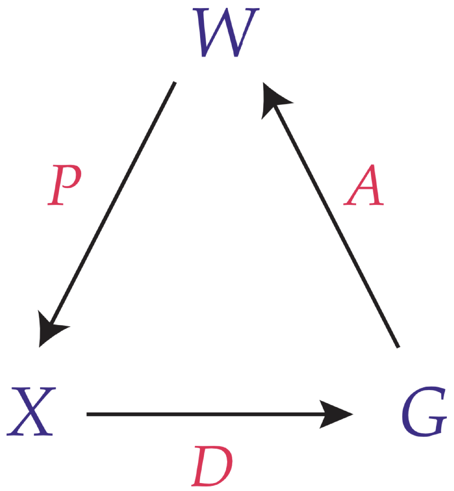
Figure 2.
Geometry of trace chain theorem.
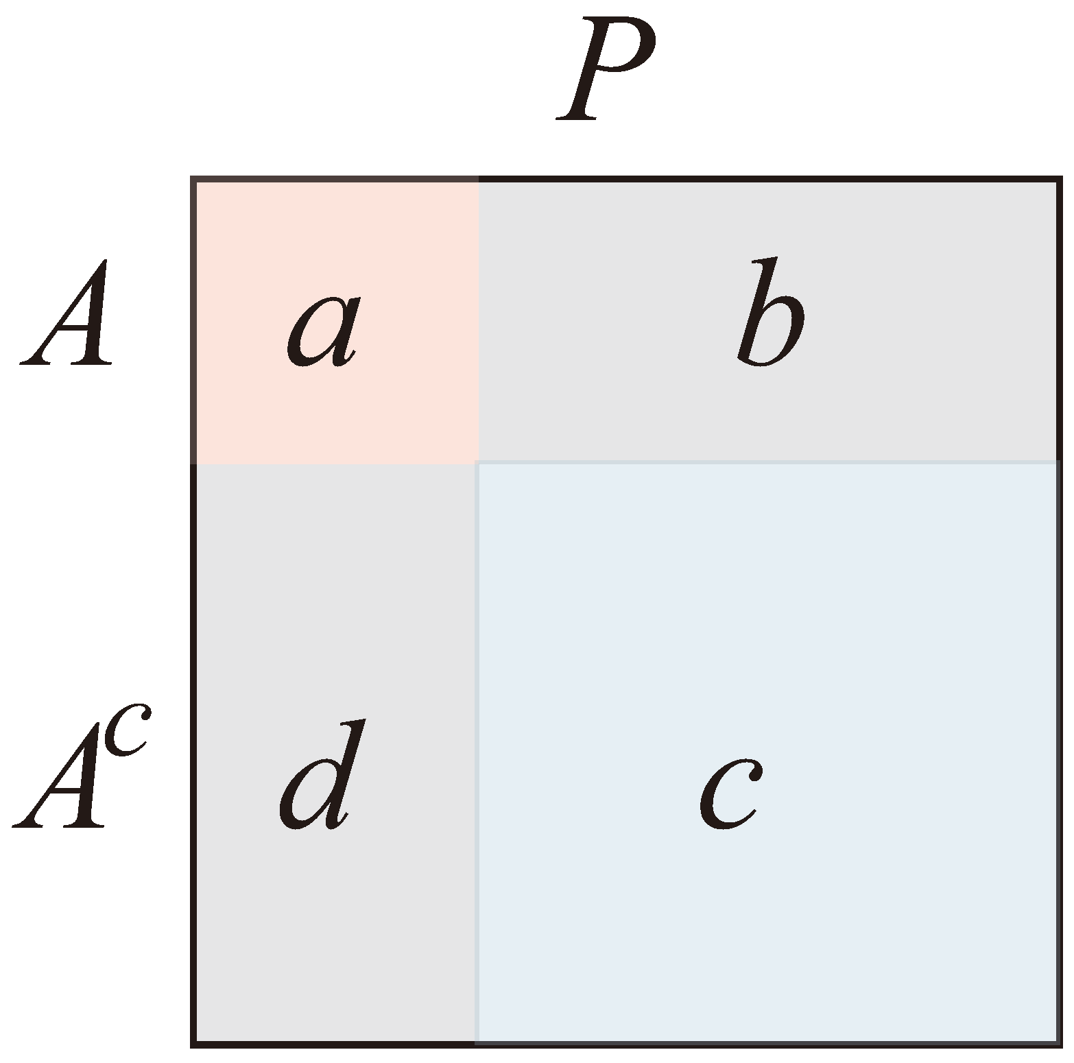
Figure 3.
Traces as spatial windows.
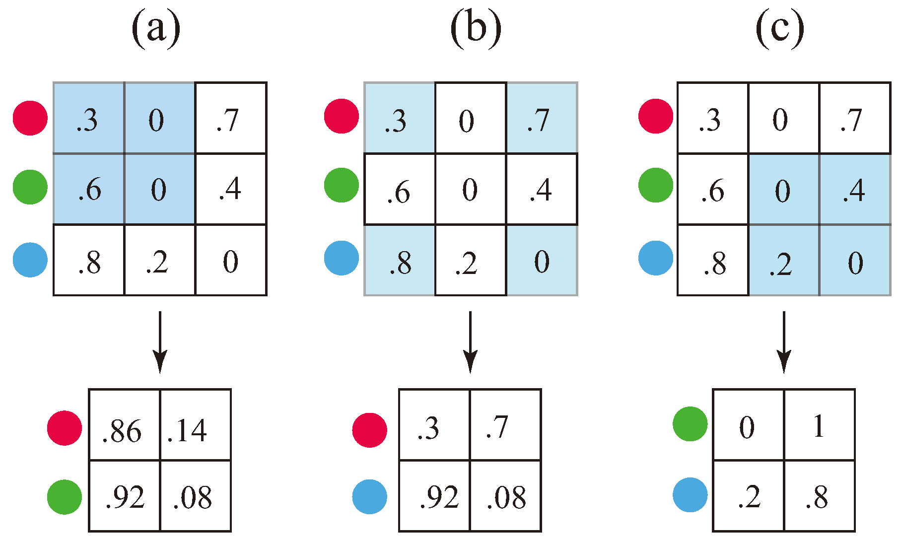
Figure 4.
The Lebesgue order.
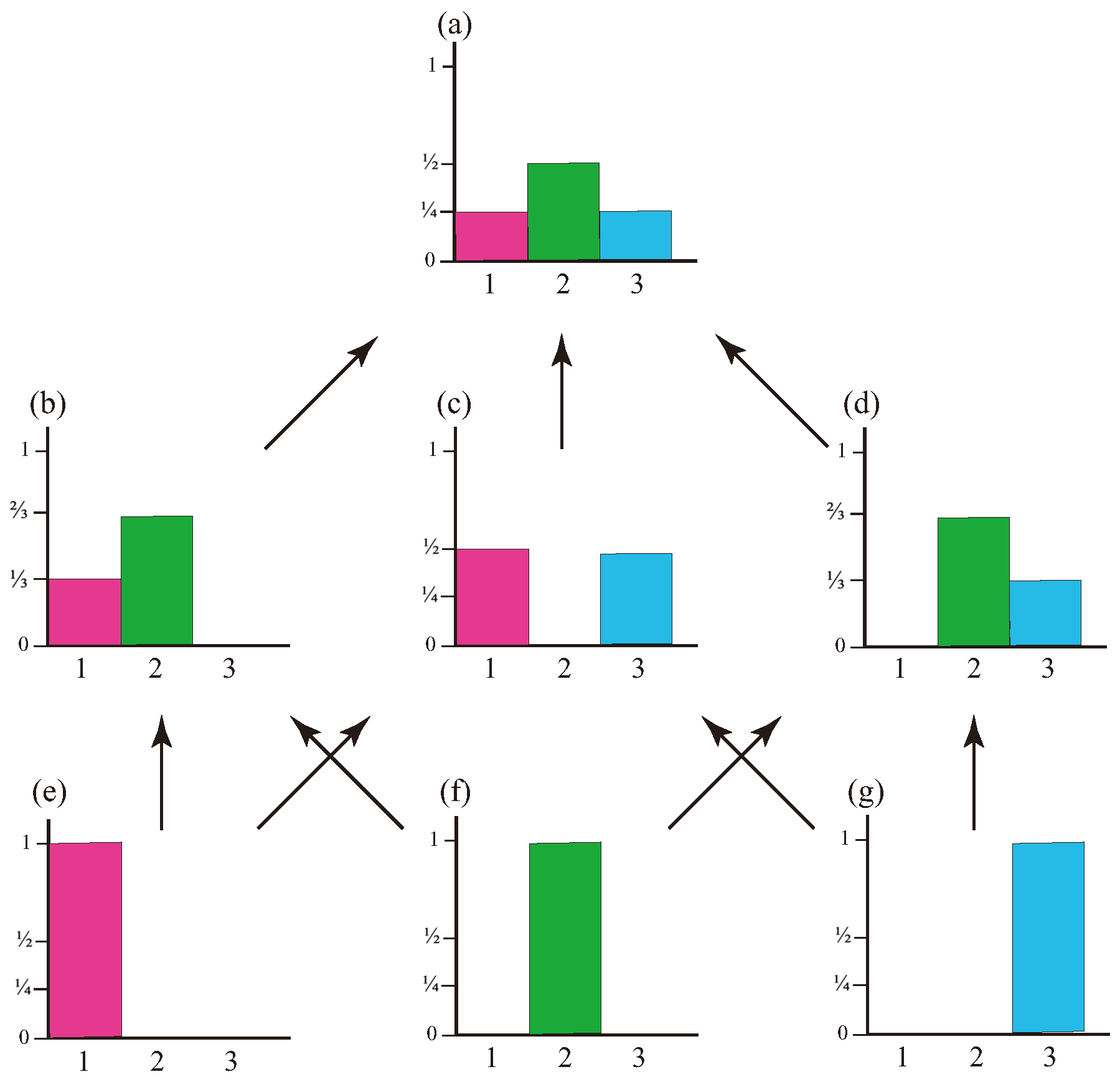
Figure 5.
The homomorphism from the trace order to the Lebesgue order.
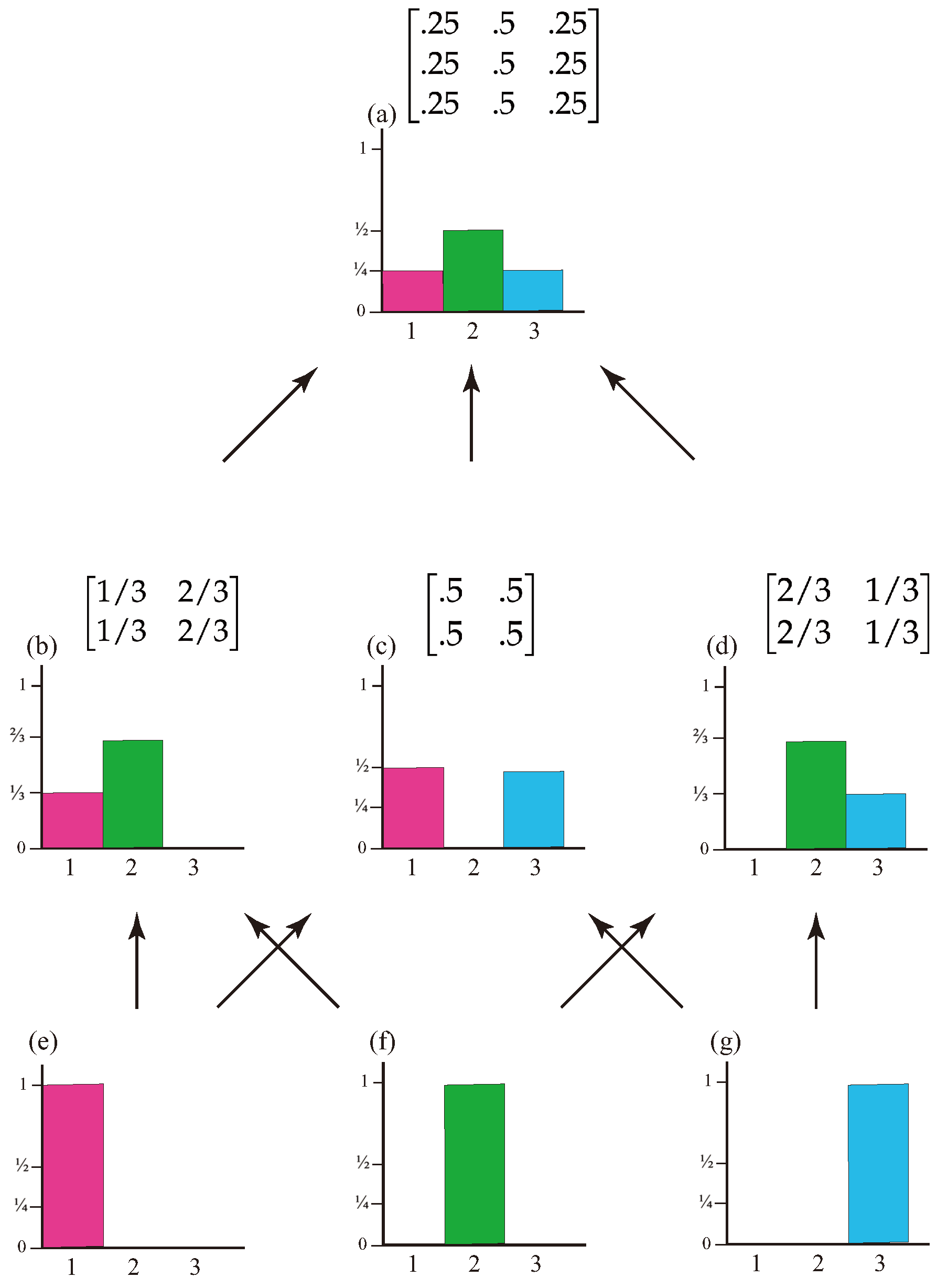
Figure 6.
Plot of the entropy rates for all Markov kernels.
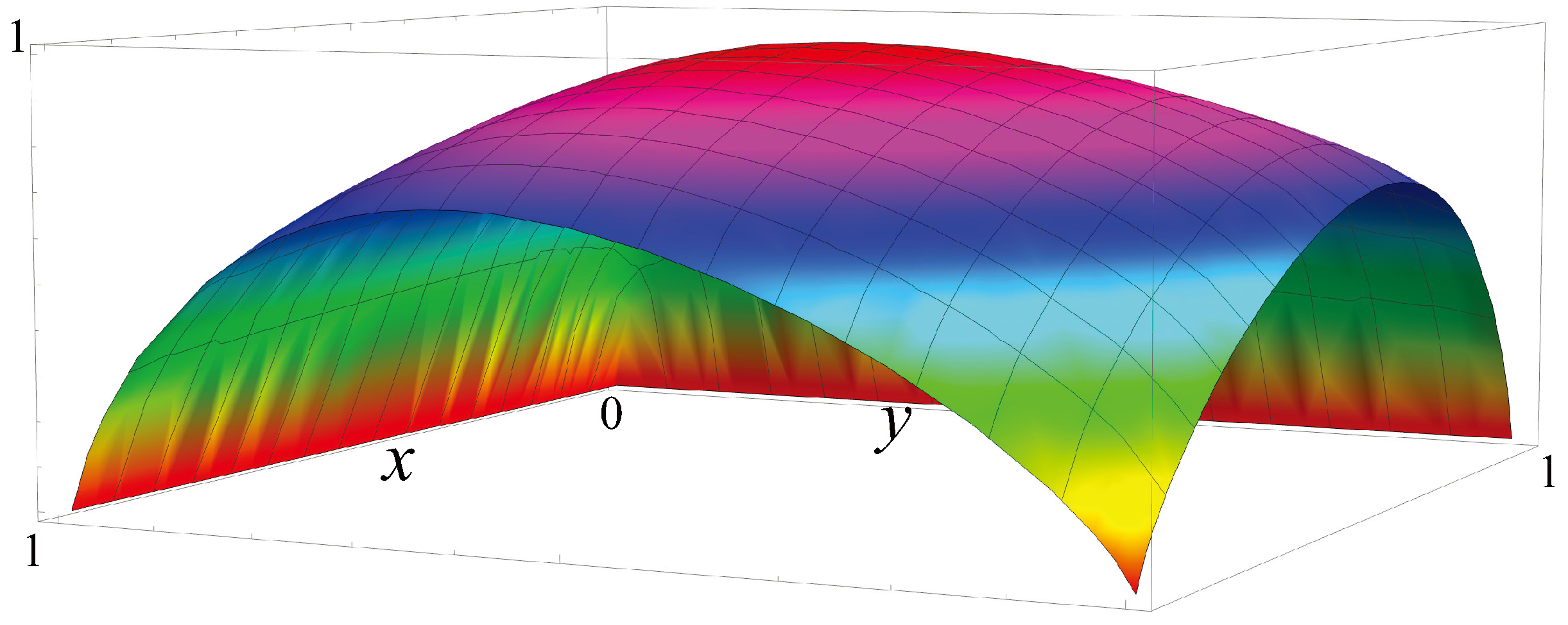
Figure 7.
Top-view plot of the entropy rates for all Markov kernels, with iso-mass contours.
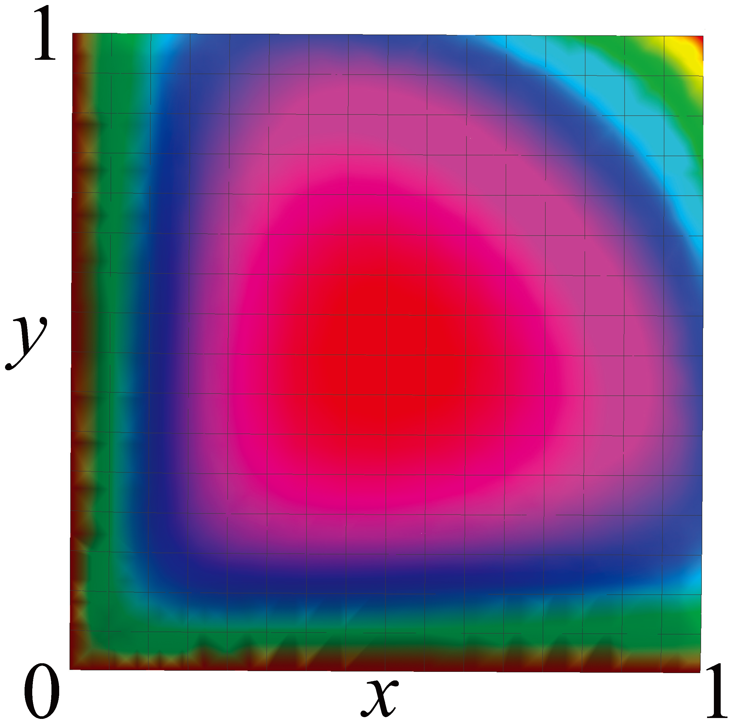
Figure 8.
Determinants for all Markov kernels. Determinants are on the vertical axis. is the horizontal rectangle in the middle.
Figure 8.
Determinants for all Markov kernels. Determinants are on the vertical axis. is the horizontal rectangle in the middle.
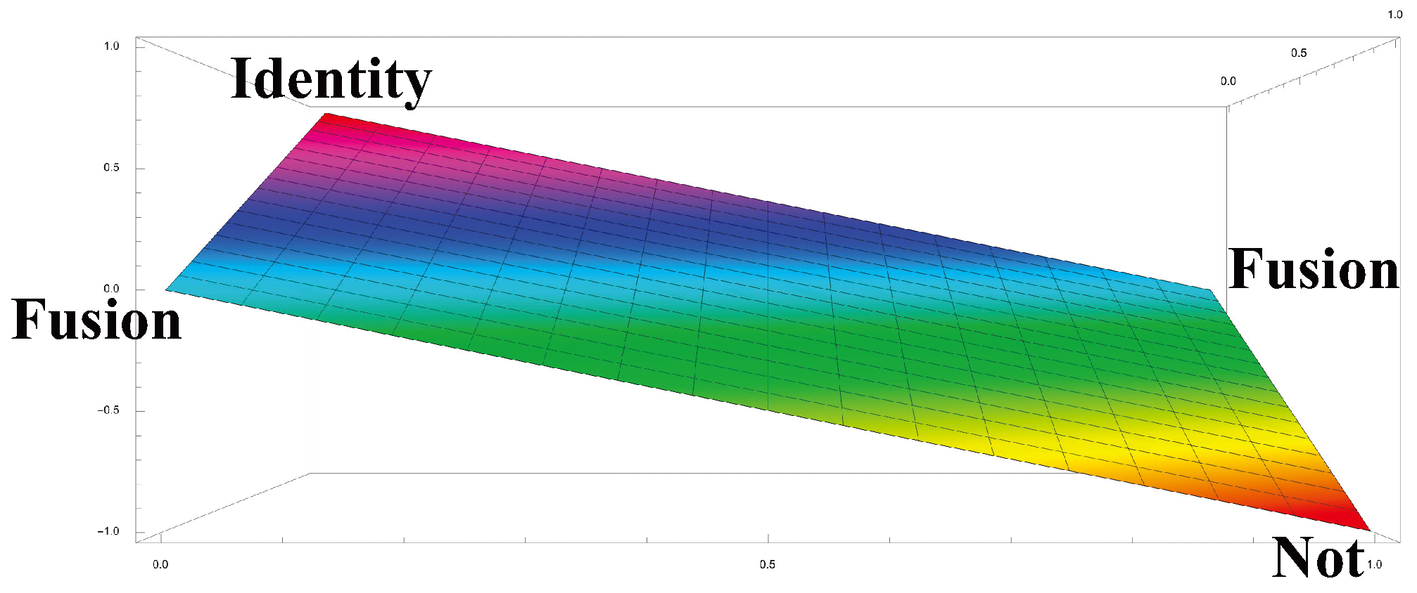
Figure 9.
Commute times for all Markov kernels. Commute times are on the vertical axis. is the bottom rectangle.
Figure 9.
Commute times for all Markov kernels. Commute times are on the vertical axis. is the bottom rectangle.
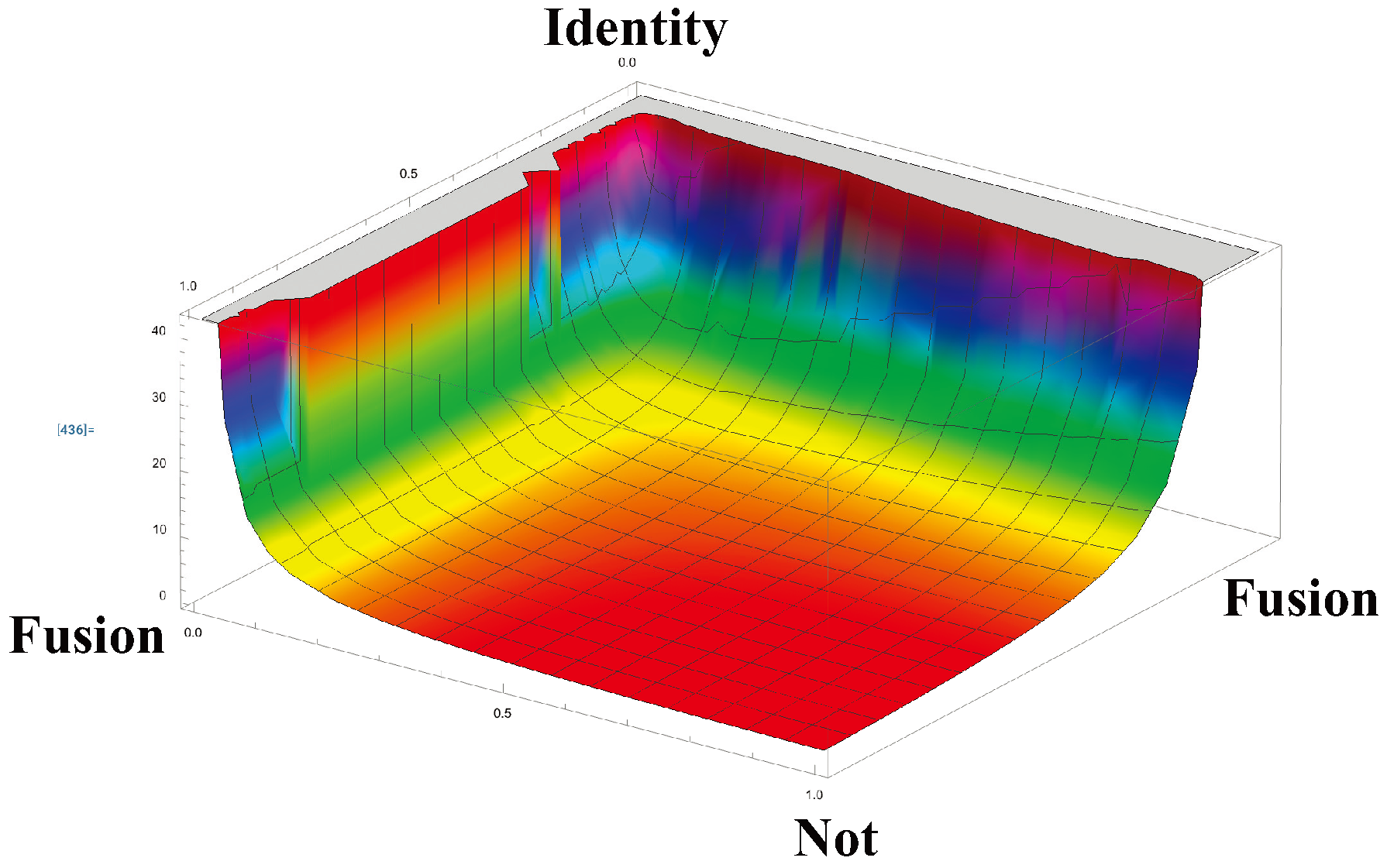
Figure 10.
Markov matrices corresponding to free, bound, and confined particles.
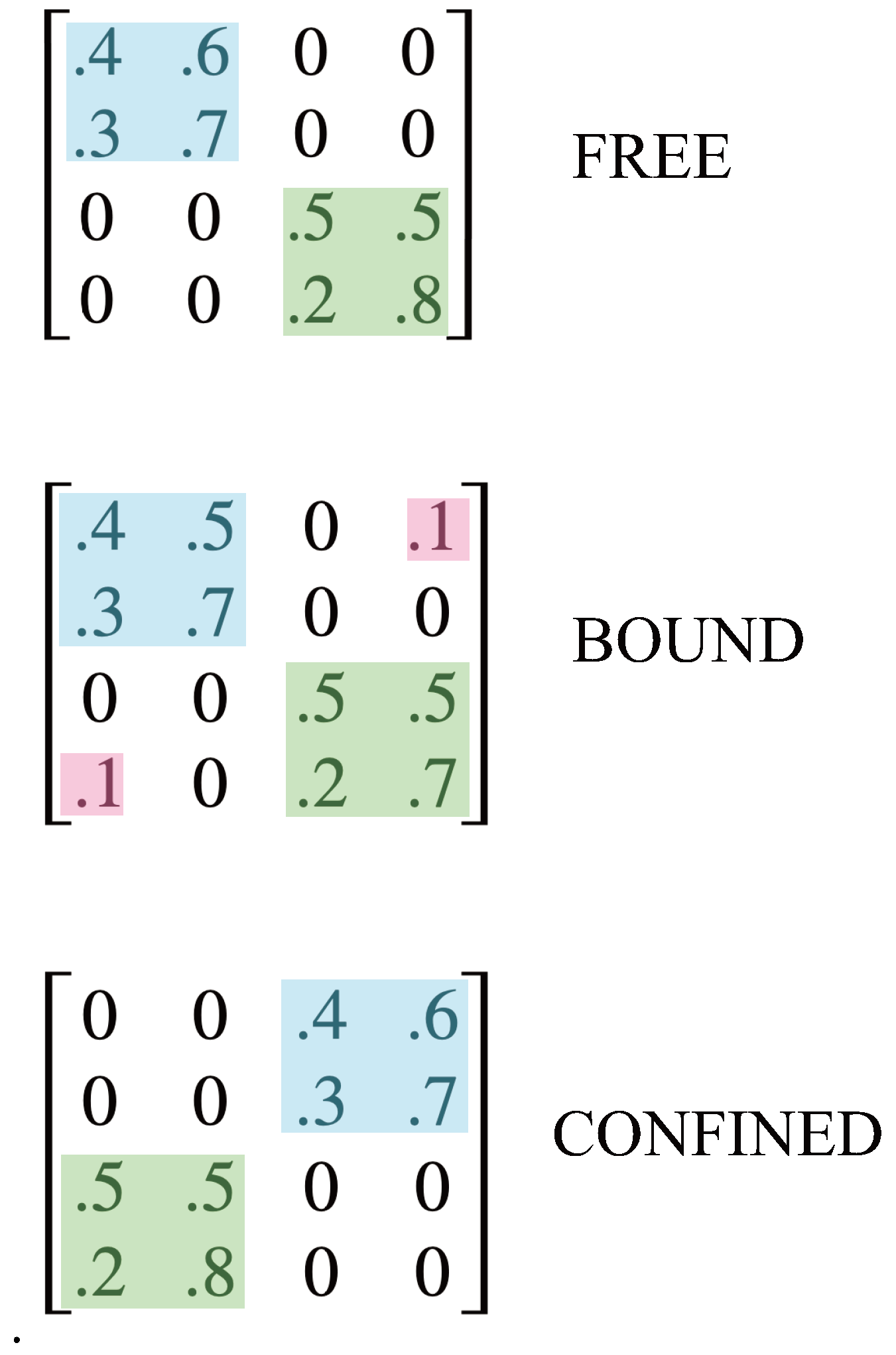
Figure 11.
Markov graphs corresponding to free, bound, and confined particles.
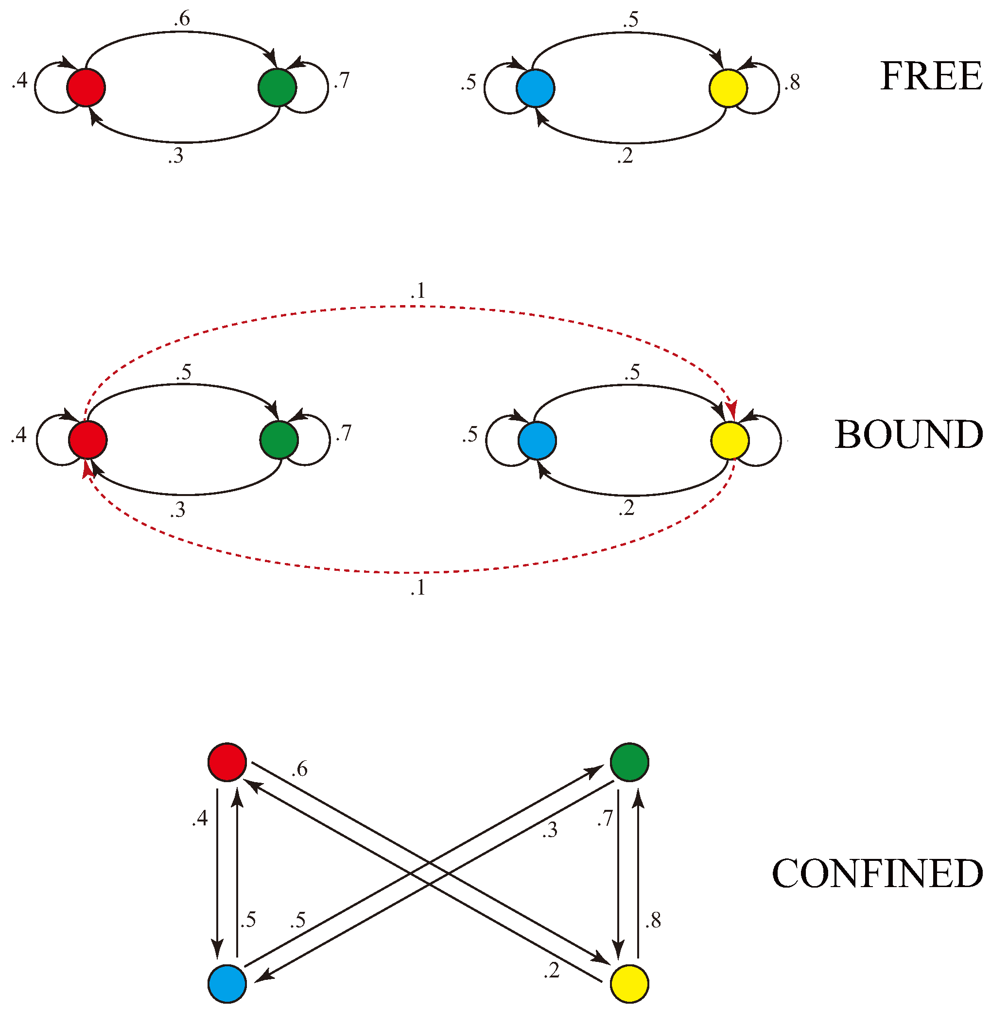
Figure 12.
Graphic representations of the outer product of three vectors, . The circles with arrows indicate the orientations of the pairwise outer products.
Figure 12.
Graphic representations of the outer product of three vectors, . The circles with arrows indicate the orientations of the pairwise outer products.
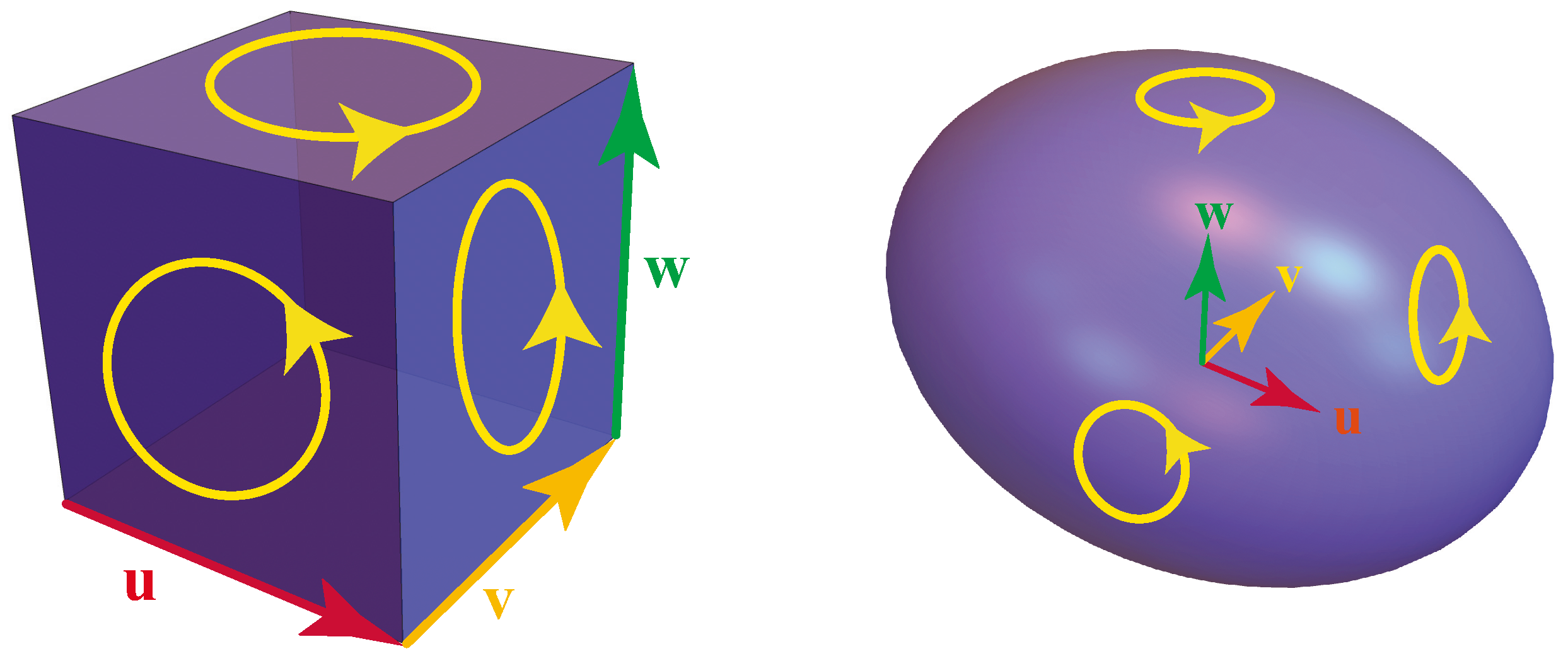
Figure 13.
Graphic representation of the C-spin axis of a Markovian kernel Q.
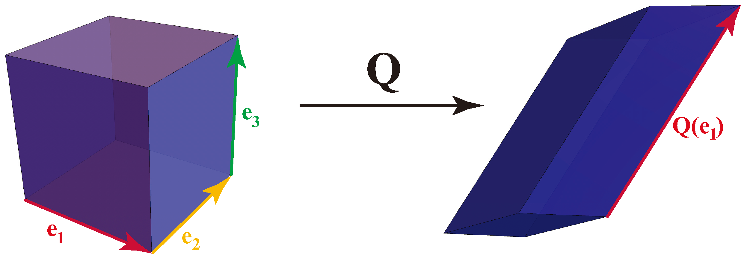
Figure 14.
The C-spin axis for each Markovian kernel of as given by the transformation .
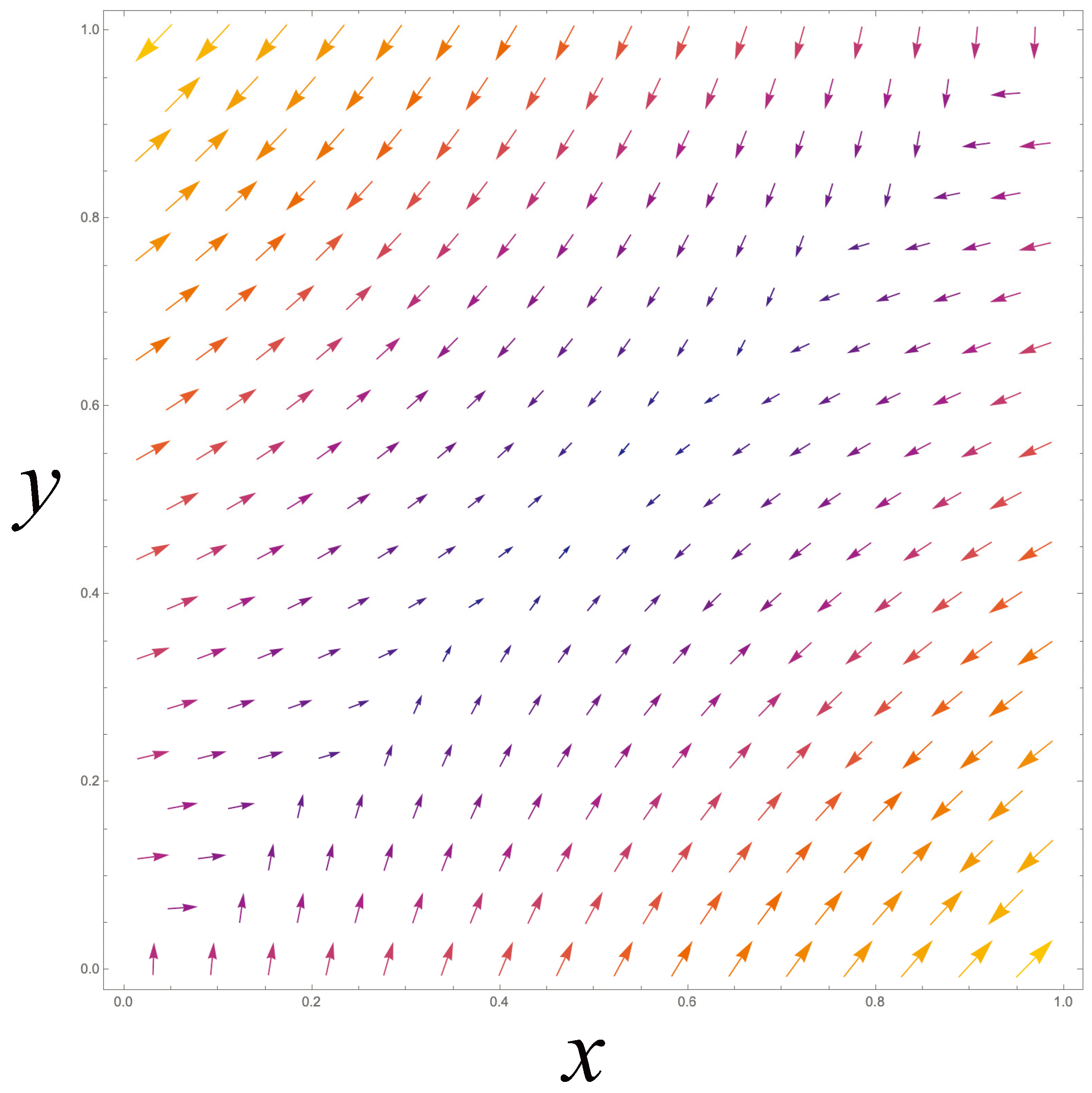
Disclaimer/Publisher’s Note: The statements, opinions and data contained in all publications are solely those of the individual author(s) and contributor(s) and not of MDPI and/or the editor(s). MDPI and/or the editor(s) disclaim responsibility for any injury to people or property resulting from any ideas, methods, instructions or products referred to in the content. |
© 2024 by the authors. Licensee MDPI, Basel, Switzerland. This article is an open access article distributed under the terms and conditions of the Creative Commons Attribution (CC BY) license (http://creativecommons.org/licenses/by/4.0/).
Copyright: This open access article is published under a Creative Commons CC BY 4.0 license, which permit the free download, distribution, and reuse, provided that the author and preprint are cited in any reuse.


